Optimum Design of a Standalone Solar Photovoltaic System Based on Novel Integration of Iterative-PESA-II and AHP-VIKOR Methods

Abstract

Solar energy is considered one of the most important renewable energy resources, and can be used to power a stand-alone photovoltaic (SAPV) system for supplying electricity in a remote area. However, inconstancy and unpredictable amounts of solar radiation are considered major obstacles in designing SAPV systems. Therefore, an accurate sizing method is necessary to apply in order to find an optimal configuration and fulfil the required load demand. In this study, a novel hybrid sizing approach was developed on the basis of techno-economic objectives to optimally size the SAPV system. The proposed hybrid method consisted of an intuitive method to estimate initial numbers of PV modules and storage battery, an iterative approach to accurately generate a set of wide ranges of optimal configurations, and a Pareto envelope-based selection algorithm (PESA-II) to reduce large configuration by efficacy obtaining a set of Pareto front (PF) solutions. Subsequently, the optimal configurations were ranked by using an integrated analytic hierarchy process (AHP) and vlsekeriterijumskaoptimizacija i kompromisonoresenje (VIKOR). The techno-economic objectives were loss of load probability, life cycle cost, and levelized cost of energy. The performance analysis results demonstrated that the lead–acid battery was reliable and more cost-effective than the other types of storage battery.

1. Introduction

The electricity demand is rapidly increasing due to growth in population and the risk of increasing electricity bills and tariffs. These issues lead to encourage energy system designers to a transformation of technology in terms of “leaving the grid” or “living in off-grid” [1,2]. The standalone photovoltaic (SAPV) system is considered one of the most important renewable, sustainable, clean, and environmentally friendly energy sources. 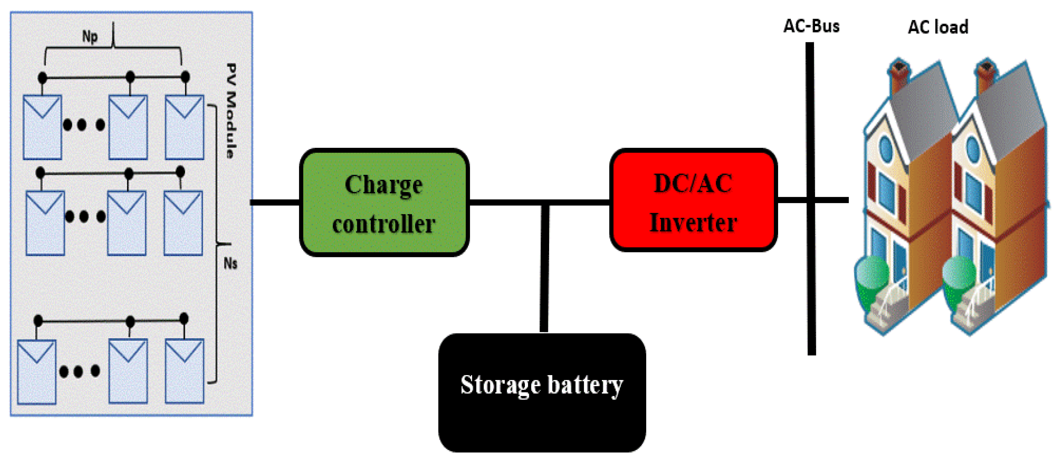However, SAPV systems need to be optimally designed in order to maximize their reliability and minimize the total cost of the system [3,4,5,6]. Therefore, an efficient sizing of a SAPV system is essential in order to supply the demanded electricity. The optimal design of the SAPV system strongly depends on the availability of the meteorological and hourly load demand. In addition, it is necessary for it to be developed on the basis of technical, economic, and environmental criteria so that the number of photovoltaic (PV) arrays, number of the storage batteries, the capacity of the converter and inverter, and the PV tilt angle should be carefully chosen.

In typical standalone off-grid PV systems, the storage battery plays a significant role not only in increasing the reliability of the SAPV system but also in reducing the total capital cost during a specific period of time. Therefore, the storage battery should be optimally chosen in order to operate on the basis of a high level of reliability and lowest cost. Accordingly, Elena et al. [7] compared three types of storage batteries in order to choose a well-suited one for the off-grid renewable energy systems. The types of storage batteries used were lead–acid, lithium cobalt oxide (LCO), LCO-lithium nickel manganese cobalt oxide composite (LCO-NMC), and lithium-ion phosphate (LFP). Experiment measurements were performed using a current of PV array and wind turbine. The results in [7] indicated that LFP battery is more accepting of variable charges and more cost-effective. However, the authors of [7] did not consider the life cycle cost period for the system. In [8], the authors studied the impact of increasing suppressed demand (SD) by 20% and 50% in three remote applications: a household, a school, and a health center in Bolivia. Loss of power supply probability (LPSP) was employed in order to calculate the reliability of the system, and the cost of the PV system hardware was set as 2.5 USD/$W_p$. The authors of [8] claimed that for the household and school, increasing the PV capacity was more cost-effective, but this led to raising the battery aging rate using a lithium-ion battery. However, the supplied energy to the load demand depends on the energy generated by the PV arrays to the storage battery, which may lead to reduction of the lifetime of the battery by increasing the capital cost. Moreover, the cost of the system’s components was assumed as being constant.

Various methods have been carried out by researchers to optimize the sizing of the SAPV system such as intuitive, numerical, analytical, artificial intelligence, and hybrid methods [9,10,11,12]. In light of optimally sizing of the SAPV system, multi-objectives optimization methods can rarely be found in the literature. In addition, the used methods based on the single objective can only candidate one optimal solution in each generation. Furthermore, simple theoretical correlations are utilized in determining the parameters of the PV module in a standard test condition (STC). The technical objective functions that have been presented in [13,14,15,16,17,18,19] to find the optimal size of the SAPV system are: loss of power supply probability (LPSP), loss of load probability (LLP), loss of load (LL), and state of charge (SOC) as technical parameters. On the other hand, life cycle cost (LCC), net present cost (NPC), value of loss load (VOLL), and levelized cost of supplied and loss energy (LCoSLE) are used as economic parameters. Therefore, it is important to consider converge, convergence, and diversity of the optimal Pareto front (PF) solutions when dealing with multi-objective optimization. There are many multi-objective evolutionary algorithms that have been proposed by researchers to find a set of PF solutions such as NSGA-II [20], PAES [21], SPEA2 [22], Pareto envelope-based selection algorithm (PESA-II) [23], and others found in reference [24]. However, it is evident that some of these methods cannot always conduct an efficient set of PF solutions, especially when the multi-objective optimization problems are complex [25].

An optimum design of the SAPV system from the set of PF solutions should be properly chosen on the basis of techno-economic objectives. Therefore, the multi-criteria decision making (MCDM) techniques are considered a suitable choice in solving energy selection problems by enabling the decision-maker to order the set of optimal solutions based on conflicting criteria [26]. However, suitable weight values should be appropriately given to the criteria according to their importance.

The rest of the paper is organized as follows. In Section 2, a background on the utilized methods for sizing of the SAPV system is presented. The description and steps of modeling the standalone PV system with it is components is presented in Section 3. Section 4 presents the techno-economic criteria that are employed in order to evaluate the performance of the SAPV system. In Section 5, the methodology presents five combined methods used to find an optimum configuration of the SAPV system using three types of the storage batteries. Section 6 presents the results, discussions, and limitations. Finally, the conclusion and future work directions are discussed in Section 7.

2. Background

Optimization Methods

Indeed, the intuitive method utilizes simplified calculations without considering the fluctuation of meteorological data and the nonlinearity relationship between subsystems [10]. In addition to this, the output-generated power of the PV arrays is calculated during the designing period that is related to safety factor, which the safety factor is chosen by the user [27,28]. Ghafoor et al. [29] proposed a sizing method to optimal the size of an off-grid PV system in Pakistan. A simple mathematical method was used to estimate the output power of PV arrays. Moreover, the average daily meteorological data were used to minimize the annualized life cycle cost (ALCC), and the technical criteria was not revealed.

To overcome the limitations of the intuitive methods, analytical methods are used for this purpose. In an analytical method, a relationship is proposed as being compatible with the reliability and size of the SAPV system. The performance of the SAPV system can be evaluated for a various set of the feasible size of system components. Then, the optimal configuration is selected by comparing single or multiple performance indices of various sets of configurations. The sizing of the PV system can be characterized by a simple calculation. Meanwhile, the major drawback is in finding the coefficients of the equation of the standalone PV system [30,31,32,33]. Riza in 2015 [34] presented a sizing methodology of PV panel and battery capacity in the SAPV system with a lighting load in Malaysia. The design space approach was obtained for sizing the curve of the PV system and storage battery configuration using three objectives: LPSP, LCC, and excess energy. According to the authors, the proposed method in [34] offered an advantage because the user can select the realistic available PV array and storage battery size configuration. However, simple component models for the system model were used, which affected the result of the output because these models cannot give the variation of the realistic metrological data. Thus, the system may be over/under-sizing, leading to increase in the capital costs or decrease in the reliability of the entire system.

In general, the most used method for sizing of the SAPV system is the numerical method due to it is accuracy and ability to discover all the design space [10]. This method takes a long period of time in implementing the system simulation. The numerical method can be classified into two parts, which are stochastic (deterministic) and probabilistic approaches [10,35]. The probabilistic approach is preferred because the uncertainty of the meteorological data is considered, in which the performance of the system can be more reliable and accurate than the stochastic approach. Moreover, the energy availability of the system can be represented in a quantitative manner [15,36,37,38]. In the numerical method, the various number of the PV arrays and storage battery configurations are conducted in the design space. Then, each pair of the PV arrays and storage batteries are simulated on the basis of hourly meteorological data and the objective function to estimate the desired configuration at a defined level of reliability of the system. Then, the lower cost from the set of configurations is selected on the basis of the objective function as an optimal solution [39]. Daily meteorological data and simple PV modules were used in these research works [13,14,15,16,17,18,19,40] to find the current-voltage (I–V) data curve at different operation conditions. The daily meteorological data were used in [13,14,15,16,17,18,40] lead to give unsatisfactory performance of the system.

Meanwhile, other studies used heuristic techniques in order to find the optimal size of a SAPV system using techno-economic objective functions such as artificial bee colony (ABC) [41], genetic algorithm (GA) [42,43], generalized regression neural network (GRNN) [44], firefly (FL) [45], and particle swarm optimization (PSO) [46]. The main advantage of these searching algorithms is the ability to converge the optimal solution in a short time. Thus, heuristic techniques can overcome the drawback of numerical algorithms. In addition to that, some of the studies combined two or more in order to enhance the converge to the optimal values and reduce the execution time, such as the research works presented in [43,47,48]. Hussein et al. [46] proposed an optimal design of the SAPV system using multi-objective particle swarm optimization (MOPSO) in Malaysia. Two variants of the PSO algorithm were presented with reference to a sigmoid function PSO ($SFPS{O}_{cf})$ and adaptive weights PSO $(AWPS{O}_{cf})$ using techno-economic criteria. The performance results demonstrated that the $SFPS{O}_{cf}$ algorithm has a trivial superiority in selecting an optimal configuration in terms of accuracy. However, the main demerit of the method proposed in reference [46] the use of a non-scale (NS) approach that can conduct only one solution on the basis of given weights. In addition, the proposed algorithm cannot cover all the Pareto front (PF) solution when all possible status of weights within [0,1] are considered.

On the basis of the literature review, the proposed numerical methods in [13,15,16,18,36,37,38,39,40,49] do not simultaneously solve multi-objective optimization for the sizing of the SAPV system, which is considered as a theoretical gap in the presented study. Therefore, the real challenge is to obtain a set of optimal solutions called the Pareto optimal solutions front. However, the challenge is in providing solutions close to the true PF (convergence), finding well-distributed solutions on the PF (diversity), and covering maximum PF (coverage). In [43], a set of optimal configurations was generated using the NSGA-II algorithm for the SAPV system based on two types of storage batteries: lead–acid and lithium-ion. However, NSGA-II may fail in establishing an accurate PF solution due to the obtained aggregation method [24,50]. Moreover, the authors in [50] proposed three scenarios in order to optimally determine the size of the SAPV system on the basis of a salp swarm algorithm considering techno-economic criteria. The results demonstrated that the multi-objective salp swarm non-dominated roulette wheel (MOSS-NDRW) scenario outperformed others in terms of converge and convergence.

As a matter of fact, the aim of establishing a set of PF solutions is to choose the final “best solution” alternative. Therefore, MCDM techniques have been applied in order to provide a preferred structure according to the relative importance of criteria [51]. To rank alternatives, the technique for order preference by similarity to ideal solution (TOPSIS) and vlsekeriterijumskaoptimizacija i kompromisonoresenje (VIKOR) are suitable in order to determine the best feasible solution for the decision-maker [52]. Both methods are efficient in order to use when the quantity data and objective are given. In TOPSIS method, the alternatives can be ordered based on the shortest and farthest distances from the ideal to the negative ideal solutions, respectively. From this view, in [53], the authors proposed a population-based differential evolution (DE) method in order to construct a set of optimal solutions based on NSGA-II, then AHP integrated with TOPSIS was used to select the optimal solution from a set of PF solutions. However, the relative importance is not considered by TOPSIS [54]. On the other hand, VIKOR is functionally associated with discrete alternative problems, making it a more practical technique for tackling real-world problems [55]. Moreover, VIKOR can rapidly select the best alternative from many alternatives and attributes. However, the main obstacle of the VIKOR approach is in the selection of appropriate weight and checking judgment consistency. Thus, AHP is a convenient technique for acquiring the relative importance of various criteria.

In this study, a novel integration of the Iterative-PESA-II and AHP-VIKOR method was developed in order to select the optimum size of the SAPV system. Firstly, the intuitive method was obtained for rough calculation of numbers of PV modules and storage batteries. Then, the iterative approach computed the number of PV modules that were connected in series and parallel. Moreover, the size of the SAPV system was optimally considered on the basis of the techno-economic criteria of LLP, LCC, and levelized cost of energy (LCE). In this proposed sizing approach, the favorable level of reliability was defined in order to find a set of SAPV system configurations using hourly meteorological data for one year. After that, the Pareto envelope-based selection algorithm (PESA-II) method was utilized in order to nominate a set of optimal configurations to construct optimal PF solutions. Subsequently, the integrated AHP-VIKOR technique was proposed in order to rank and choose the optimum configuration of the SAPV system. The proposed hybrid approach overcame all the drawbacks of intuitive, analytical, numerical, and stochastic methods that were faced in the sizing of the SAPV system. Finally, an accurate single-diode (SD) PV model was used to establish the I–V characteristic curve, which can give a realistic evaluation for the extracted energy of the PV array. The proposed method showed a high level of reliability and low cost in designing a SAPV system.

3. Standalone PV System

A typical SAPV system mainly comprises the PV arrays that convert the sun’s rays to a DC current; the storage battery can be used for storing the excess energy and power conditioner units containing a DC–DC converter and a DC–AC inverter. Figure 1 depicts a typical standalone PV system.

3.1. Single-Diode Model

The most commonly used representation of the performance of the output current of the PV module is the single-diode model. This is due to it is simplicity, accuracy, and ability to reflect the actual behavior of the PV cells, as illustrated in Figure 2. For instance, the single-diode PV model offers a high ability in reflecting reality behavior when it is dealing with non-linearity and stochastic nature among other mathematical models [56]. The single-diode model consists of current $I$ and voltage $V$ as the outputs current and voltage of the PV module; photocurrent $I_{Ph}$, which has a high sensitivity to environmental conditions; the diode reverse saturation $I_o \left(\mathrm{in} \mathrm{A}\right)$; and the parallel and series resistances $R_p$ and $R_s$, which represent the losses of the PV solar cell ($\mathsf{\Omega }$). Thus, the following equation represents the output current of the single-diode PV module:

$$I=I_{Ph}-I_o\left[exp\left(\frac{V+I{R}_s}{V_t}\right)-1\right]-\frac{V+I{R}_s}{R_p}$$

(1)

where $V_t$ refers to the diode thermal voltage (in V) and can be represented as

$$V_t=\frac{dKB{T}_c}{q}$$

(2)

where $d$ is the ideality factor of the diode, $KB$ refers to the Boltzmann constant (1.3806503 × 10⁻¹⁹ J/K), $T_c$ is the cell temperature ($K$), and $q$ represents the electron charge (1.60217646 × 10⁻¹⁹ Coulombs). The five parameters ($I_{Ph},$ $I_o,$ $R_s,$ $R_p$, and $d$) need to be extracted accurately.

Furthermore, the PV array consists of parallel $N_p$ and series $N_s$ modules. Therefore, the output current of the PV array is expressed as follows:

$$I=N_p{I}_{Ph}-N_p{I}_0\left[exp\left(\frac{1}{V_t}\left(\frac{V}{N_s}+\frac{I{R}_s}{N_p}\right)\right)-1\right]-\frac{N_p}{R_p}\left(\frac{V}{R_p}+\frac{I{R}_s}{N_p}\right)$$

(3)

where $I$ and $V$ are the output current (A) and voltage (V) of the PV array, respectively. The five parameters ($I_{Ph},$ $I_o,$ $R_s,$ $R_p$, and $d$) are extracted by the improved electromagnetism-like (IEM) algorithm [57]. The accuracy of the IEM algorithm can be represented by establishing current-voltage (I–V) and power-voltage (P–V) characteristic curves, which are shown in Figure 3a,b. The efficiency of the PV array is computed by the following equation:

$${\eta }_{PV}=\frac{VI}{AG}$$

(4)

where $A$ denotes to the PV array’s area $\left({\mathrm{m}}^2\right)$, and $G$ represents the amount of the solar irradiation fall on the surface of the PV array $\left(\mathrm{W}/{\mathrm{m}}^2\right)$. The type of the used PV module is a Kyocera KC120-1 multi-crystalline silicon, which was used in this research study. To simulate the output power of the PV array, a maximum power point tracker (MPPT) was employed in this study as shown in

Table 1. Extracted five parameters of single-diode PV model at the MPPT.

Solar Radiation (W/m2)	Cell Temperature (k)
978	328.56
Parameters	Values
$a$	1.3257
$R_s$	0.2140
$R_p$	38.5131
$I_{Ph}$	6.3930
$I_o$	5.9134 × 10−6
Average value of RMSE	0.0589

.

3.2. Battery Mathematical Model

Various types of storage battery capacity (kW) were proposed in this study in order to verify those most effective and suitable for the SAPV system. Therefore, the days of autonomy are given by the following [58]:

$$C_{bat}=\frac{E_{Load}\ast AD}{DOD\ast \eta b\ast \eta inv}$$

(5)

where $C_{bat}$ represents the capacity of the storage battery; $AD$ refers to number of the autonomy days (typically between 3–5 days) [13]; $E_{Load}$ represents the required load demand; and $DOD\ast \eta b\ast \eta inv$ are the depth of discharge (80%), efficiency of the storage battery (85%), and efficiency of the inverter (95%). The state of chare of the battery (SOC) can be expressed by [36]

$$E_{bat}=SOC\left(t-1\right)+\left[P_{pv}\left(t\right)-P_{load}\left(t\right)\right]$$

(6)

$$SOC\left(t\right)=\{\begin{array}{c}SO{C}_{min}, E_{bat}<SO{C}_{min}\\ E_{bat}, SO{C}_{min}<E_{bat}<SO{C}_{max} \\ SO{C}_{max}, E_{bat}>SO{C}_{max}\end{array}$$

(7)

where $P_{pv}\left(t\right)$ and $P_{load}\left(t\right)$ refer to the hourly output energy generated by PV modules and energy required by the load, $SOC\left(t-1\right)$ and $SOC\left(t\right)$ represent the status of the state of charge (SOC) for the battery at initial and final points of charging and discharging, respectively; and $E_{bat}$ denotes the battery hourly capacity. For a more reliable and longer lifetime for the storage battery, the minimum energy stored in the battery must be pointed as given by the following:

$$E_{bat\_min}=SO{C}_{max}\ast \left(1-DOD\right)$$

(8)

The required energy supposed to be stored in the battery can be written by the following equation [13]:

$$E_{bat}=\left({\displaystyle \sum }_{i=1}^{365}energy excess-{\displaystyle \sum }_{i=1}^{365}energy deficit\right). \eta ch$$

(9)

where $\eta ch$ represents the battery’s charging efficiency.

3.3. Load Profile

In this work, the hourly load demand of a typical house in a rural area in Malaysia was considered, which can be found in details in the load demand in [46]. The proposed hybrid method was analyzed using hourly meteorological data for one year. Furthermore, the data used was taken from Subung meteorological station in Subung Jaya, Klang Valley, Malaysia (latitude $3.12°$ north and longitude $101.6°$ east) [46].

4. Proposed Criteria for the Sizing of the SAPV System

In order to obtain the optimal configuration of the SAPV system, the number of PV modules (in series ($N_s)$ and parallel ($N_s)$) and the number of the storage battery ($Bat$) should be chosen accurately by considering techno-economic criteria. Therefore, three important criteria, namely, loss of load probability (LLP), life cycle cost (LCC), and levelized cost of energy (LCE), were chosen to increase the reliability and minimize the total cost of the system. In this study, the objective function $(\mathrm{F}\left(\mathrm{X}\right)$) of the problem could be obtained by simultaneously minimizing LLP, LCC, and LCE. Thus, the multi-objective optimization (MOOP) to optimally size of the SAPV system can be described by the following equations [59]:

$$\begin{array}{c}Min F\left(X\right)=\left\{LLP,LCC,LCE\right\}\\ X=\left(N_s,N_P,Bat\right)\end{array}$$

(10)

where $X$ is the vector of the decision variables that should be optimized by the proposed method.

4.1. Loss of Load Probability

The availability of the system can be measured by using LLP, which is defined as the ratio of the energy deficits to the required load demand during a specific period of time [60]. The range of the LLP’s values are between 0 and 1. Thus, high reliability could be chosen for optimal sizing of the SAPV system when it was close to 0. LLP can be represented by the following equation:

$$LLP=\frac{{{\displaystyle \sum }}_1^{12\ast 365}Energy deficit{s}_i}{{{\displaystyle \sum }}_1^{12\ast 365}Energy deman{d}_i}$$

(11)

4.2. Life Cycle Cost

The best indicator to evaluate the capital cost of the system with it is components was the life cycle cost (LCC). Thus, LCC was used to compute four parts of the SAPV system which were PV panels, converter, storage battery, and inverter. Moreover, LLC considered the initial total cost values $\left(I{C}_{tot}\right)$, replacement cost values $\left(C_{rep}\right)$, and operation, as well as maintenance cost values $\left(C_{O\&M}\right)$ during a period of time. The unit cost and the lifetime of the system’s components are given in

Table 2. Financial data of the three types of storage batteries [63].

Type	Cost/Unit (USD/Wp)	Lifetime (in Year)	${\mathit{C}}_{\mathit{O}\&\mathit{M}}$	${\mathit{N}}_{\mathit{r}\mathit{e}\mathit{p}}$	Module Capacity	Producers
Lead–acid	0.118	2	3%	10	1.3 KWh	Centennial
AGM	0.1723	3		7	3.2 KWh	Crown
Lithium-ion	1.08	10		1	6.6 KWh	Discover AES

. Therefore, the mathematical equations can be written by [41]:

$$LCC=I{C}_{tot}+C_{rep}+C_{0\&M}$$

(12)

The initial total cost of all components of the SAPV system was considered, which included the price of each part of the system, the installation, and the amount of the civil works. The initial total cost can be given by $\left(I{C}_{tot}\right)$, which is given by [61]:

$$I{C}_{tot}=C_{PV}\times C_{Unit,PV}+C_{Batt}\times C_{Unit,Batt}+C_{Bidi}\times C_{Unit,Bidi}+C_{CH}\times C_{Unit,CH}+C_O$$

(13)

where $C_{PV,} C_{Unit,PV}$ are total capacity and unit cost of the PV array, respectively; $C_{Batt}, C_{Unit,Batt}$ are the total capacity and unit cost of the battery, respectively; $C_{Bidi}, C_{Unit,Bidi}$ are the total capacity and unit cost of the inverter, respectively; $C_{CH}, C_{Unit,CH}$ are the total capacity and unit cost of the converter, respectively; and $\left(C_O\right)$ represents the total constant cost with including both civil work and installation cost. In this study, three components required replacement during the system lifetime, these being the storage battery, converter, and inverter. The values of the inflation rate ($FR$) and interest rate ($IR$) of the components of the system were considered in this study. Thus, the replacement cost ($C_{rep})$ can be given as [61]

$$C_{rep}=C_{Unit}\times C_{nom}{\left({{\displaystyle \sum }}_{i=1}^{N_{rep}}\left[\frac{1+FR}{1+IR}\right]\right)}^{\left(\frac{LP\ast i}{N_{rep}+1}\right)},$$

(14)

where $C_{Unit}$ represents the unit component cost of the storage battery, converter, and inverter; ($C_{nom})$ denotes to the nominal capacity of the replacement system component; and ($N_{rep}$) refers to the number of replacement of each component over the system life period ($LP$). The operation and maintenance cost $\left(C_{O\&M}\right)$ calculation can be described as [62]

$$C_{O\&M}=\{\begin{array}{c}{C_{O\&M}}_0\left(\frac{1+FR}{IR-FR}\right)\left(1-{\left[\frac{1+FR}{IR+FR}\right]}^{LP}\right) for IR\ne FR \\ {C_{O\&M}}_0\times LP for IR=FR\end{array}$$

(15)

where ${C_{O\&M}}_0$ is the operation and maintenance cost in the first year. The detailed units’ costs and services of the proposed SAPV system can be found in [61,63], whereas the units’ cost of the lead–acid, absorbent glass mat (AGM), and lithium-ion batteries are tabulated in Table 2.

4.3. Levelized Cost of Energy (LCE)

Another parameter used to represent the economic aspects of the SAPV system was LCE. LCE is defined as the ratio of the total cost of the all components of the SAPV system to the total of the conducted energy by PV arrays throughout one year, which can be given as follows [64,65]:

$$LCE=\frac{TAC}{E_{tot}}$$

(16)

where $TAC$ is the total cost of the system components and $E_{tot}$ is the total annual energy generated by the system during a specific period of time and can be represented by the following equation:

TAC = (LCC/LP)

(17)

5. The Proposed Optimization Sizing Method

In this research work, the proposed optimization of the SAPV system was based on four combined methods— the intuitive and numerical, PESA-II, and integrated AHP-VIKOR methods. The descriptions of these methods are shown in Figure 4.

5.1. Intuitive Method

The intuitive method is used to predict the number of PV modules and storage batteries. However, it was observed from the literature that the intuitive method may result in over/under-sizing of the SAPV system. Therefore, the intuitive method was applied in order to determine the ranges of search space. The number of PV modules can be calculated on the basis of the intuitive method, as follows:

$$N_{PV}=\frac{E_{Load}}{PSH{\eta }_{inv}{\eta }_{bat}A}{S}_F$$

(18)

where $E_{load}$ represents the daily energy load demand, $PSH$ is the peak sunshine hours, ${\eta }_{inv}$ and ${\eta }_{bat}$ are the efficiencies of the inverter and system, $A$ is the area of the PV array, and $S_F$ is the design safety factor. The initial capacity value of the storage battery is calculated on the basis of Equation (5). In addition to this, the number of the storage batteries in series and parallel can be calculated by the following equations:

$$N_{Sbat}=\frac{V_{bus}}{V_{battery}}$$

(19)

$$N_{Pbat}=\frac{C_{bat}}{C_{b,Wh}}$$

(20)

where $V_{bus}$ and $V_{battery}$ are the voltage bus of the system and battery, respectively, and $C_{b,Wh}$ represents the days of autonomy and W-hour capacity of the battery. Thus, the total number of the storage battery is given by multiplying the series $N_{Sbat}$ and parallel $N_{Pbat}$ numbers of batteries, and is expressed as follows:

$$N_{Tbat}=N_{Sbat}\times N_{Pbat}$$

(21)

The $N_{Tbat}$ is used to determine the design space of the storage battery. Afterward, the numerical method is used for finding a set of optimal configurations of the system.

5.2. Iterative Method

After determining the bounders of the PV modules and storage batteries numbers, the iterative method is employed by increasing the numbers of PV modules (in parallel and series) and storage battery from minimum to maximum based on predefined ranges. The operation process of energy management of SAPV on the basis of the iterative method is illustrated in Figure 5. The first step of the algorithm can be performed by obtaining the specification of the system such as the efficiency of the PV module, efficiency of charging, and discharging of the storage battery, and the efficiency of the inverter, converter, and wires. After obtaining the required specifications, which are tabulated in

Table 3. Components’ specifications of the standalone PV system.

Components	Characteristics	Value
Kyocera $KC120$-1 PV panels	Maximum power at STC	120 (W)
	Open circuit voltage	21.5 (V)
	Short circuit current	7.45 (A)
	Voltage at MPP	16.9 (V)
	Current at MPP	7.1 (A)
	No. of cells connected in series	36
	Nominal operation cell temperature	43.6 ($℃$)
Battery	Efficiency	85%
	Maximum $DoD$	80%
	Bus voltage	24 (V)
	Battery voltage	12 (V)
DC–DC controller	Efficiency	95%
DC–AC inverter	Efficiency	90%
AC voltage	Electrical load AC	230 (V)

, the simulation starts to calculate the E_net by subtracting the predicted output energy of the PV model from the energy of the load. Then, the net energy is classified in three cases, which are

• Case 1: The energy of the PV array equals the energy of the load.
• Case 2: The energy of the PV array is larger than the energy of the load.
• Case 3: The energy of the PV array is less than the load energy.

In the first case, the battery energy is not used and there is no damped or deficit energy that is equal to zero. In the second case, the energy produced by the PV array is larger than the load energy. There is an excess energy and depending on the state of charge (SOC) of the battery. If the SOC of the battery is full, the amount of excess energy will be damped. In contrast, the amount of excess energy will be used in order to charge the battery and the new value of SOC will be calculated by Equation (7) and the deficit energy is zero. In case 3, if the SOC of the storage battery is more than the minimum value $E_{bat\_min}$ (Equation (8)) then the storage battery is able to meet the load demand. The load will be supplied with/without the energy of the PV array and storage battery. Or else, if the SOC of the battery is less than the minimum value, the system cannot meet the load demand and there is deficit energy. The three-objective function of LLP, LCC, and LCE are calculated in each iteration.

5.3. PESA-II Method

Indeed, the numerical methods are most accurate due to their ability to discover all possible configurations in the design space. However, the iterative methods suffer not only from prolonged execution time but also in selecting the desired optimal configuration (global solution) due to the generated large number of configurations. The real challenge is to select a set of optimal solutions called Pareto front solutions. Therefore, the PESA-II method is abstained to handle the three objectives LLP, LCC, and LCE simultaneously. The Pareto envelope-based selection algorithm (PESA) was proposed by Corne et al. [66]. In PESA, there are two types of population: internal (IP) and external population (EP), the EP is archived to store the non-dominated solution in which a set of PF solutions can be established. In our proposed method, PESA-II concept can be explained by the following steps:

Step 1:

Reading the saved numbers of PV modules and storage batteries, then store them in the internal population (IP).

Step 2:

Reading the LLP, LCC, LCE objectives, then saving them in the objective function (OF) array.

Step 3:

Comprise the non-dominated members of IP into EP.

Step 4:

The next member of the EP (achieve) being chosen on the basis of region-based selection by assigning the three objectives’ fitness in objective space to all the hyperboxes.

Step 5:

The fewer individuals in the hyperbox being chosen as a winner for the next iteration. In this way, PESA-II can provide better convergences and diversity in a solution space than SPEA, PAES, and PESA algorithms.

In step 3, the EP always updates the non-dominated solutions and its size is set as 200. The new solution enters the EP if it is non-dominated within IP and should be not dominated by current solutions in the EP because the dominated solution will be removed from EP. According to steps 4 and 5, the selective fitness method is applied to all hyperboxes in order to choose fewer individuals on the hyperbox using binary tournament selection. By using binary tournament selection, the chance of selecting most isolated individuals (fewer individuals) will be $1-{\left(\frac{P-l}{P}\right)}^2$, assuming there are two hyperboxes in the current approximation to the PF, as illustrated in Figure 6. This means that increasing the number of individuals leads to having a high possibility of selection. Meanwhile, the chance of selecting the best individual is ${\left(\frac{m}{P}\right)}^2$. Therefore, the chance of selecting an individual from the least crowded box is more than crowded individual which can be calculated regarding to the ratio of this probability $\left(2Pl-l^2\right)/m^2$, where $l$ and $m$ are the least and most crowded boxes, respectively. In cases where the new non-dominated solutions try to enter EP when EP is over-full, the new non-dominated solutions can occupy less crowded members than the other solutions. The main advantage of PESA-II can be pointed out by using the binary tournament selection to adaptive range equalization and normalization of the OF values. Thus, this selection technique is oriented towards obtaining PF in a well-distributed manner [67]. In this method, there is no mutation or crossover phases; this is because all possible configurations have been investigated previously and there is no need to search for new regions in the search space. Therefore, the execution is performed only one time.

5.4. Integrated AHP-VIKOR Method

The main goal of proposing an integrated AHP-VIKOR method is to select one optimal solution (optimum solution) from the overall PF. Therefore, the AHP method was used in this study to calculate the weights for each criterion in a decision matrix (DM). Afterward, the VIKOR method was employed to a rank optimal configuration on the basis of preference criteria considered for practical judgment. Figure 7 demonstrates the structure of the integrated AHP-VIKOR method. The next subsection will discuss the integrated AHP-VIKOR method in detail.

5.4.1. AHP Method

The AHP method was developed by Saaty et al. [68], and is most widely used to demonstrate the priority importance of the criteria. The proper weights of criteria can be determined by using a pairwise comparison matrix on the basis of the opinion of three experts. The steps of the integrated AHP-VIKOR method are given by the following:

Step 1

The AHP method can be started after defining a hierarchy. The hierarchy includes the criteria and decision goal. The criteria used to select the optimal configuration of SAPV system are LLP, LCC, and LCE. The number of pairwise comparisons can be computed by $n\times \left(n-1\right)/2$, where $n$ is the number of criteria. The pairwise comparison matrix is tabulated in

Table 4. Pairwise comparison matrix of the three criteria based on Saaty’s scale.

Evaluators	Criteria	Extreme Importance	Very Strong Importance	Strong Importance	Moderate Importance	Equal Importance	Moderate Importance	Strong Importance	Very Strong Importance	Extreme Importance	Criteria
		9	7	5	3	1	3	5	7	9
1	LLP	✔									LCC
	LLP		✔								LCE
	LCC					✔					LCE
2	LLP					✔					LCC
	LLP		✔								LCE
	LCC	✔									LCE
3	LLP				✔						LCC
	LLP			✔							LCE
	LCC				✔						LCE

to show the importance of criteria on the basis of three evaluators. In this study, a pairwise comparison matrix is constructed on the basis of three experts. To initialize the weights, a pairwise comparison matrix can be built in the next step.

Step 2

The preferences on the three criteria obtained in AHP are considered. Normalization of each element is required in order to construct the normalized matrix [69], where each element in the (prefer order) matrix is the corresponding each element of the same matrix divided by the sum of all columns. Afterward, the aggregation vector’s elements are filled by the sum of elements of the corresponding row of the normalized matrix.

Step 3

The weights can be computed by dividing each element in the aggregation vector by taking the sum of all elements in the aggregation vector. The summation of weights for three criteria of each evaluator must not exceed 1.

Step 4

In this step, the consistency ratio (CR) is used to check if the elements of the preferred order matrix are consistent or not. The equation of CR can be written as follows:

$$CR=CI/RI$$

(22)

where $RI$ is a random index, which was chosen as 0.58 for this study, and $CI$ is the consistency index, which is computed by the following equation:

$$CI=\left(\lambda max-n\right)/\left(n-1\right)$$

(23)

where $\lambda max$ is the maximum value of the preferred order matrix and $n$ is the order of the matrix.

It is important to notice that, if the value of the CR is larger than 0.1, the pairwise comparison matrix is not consistent, and it will be ignored. The pairwise comparison matrix, normalized matrix, aggregation vector, weights vector, and consistency ratio are illustrated in

Table 5. AHP processing matrix to calculate the weights of criteria with consistency ratio values.

	Prefer Order				Normalization			Aggregation	Weight	Consistency Measure	Consistency Ratio
First evaluator	Criterion	LLP	LCC	LCE	LLP	LCC	LCE
	LLP	1.00	9.00	7.00	0.80	0.82	0.78	2.39	0.7978	3.0168	0.0060
	LCC	0.11	1.00	1.00	0.09	0.09	0.11	0.29	0.1000	3.0021
	LCE	0.14	1.00	1.00	0.11	0.09	0.11	0.32	0.1053	3.0020
	Total	1.25	11.00	9.00	1.00	1.00	1.00	3.00	1.00	0.0035
First evaluator	Criterion	LLP	LCC	LCE	LLP	LCC	LCE
	LLP	1.00	1.00	7.00	0.47	0.45	0.54	1.46	0.4865	3.0191	0.0108
	LCC	1.00	1.00	5.00	0.47	0.45	0.38	1.31	0.44	3.0157
	LCE	0.14	0.20	1.00	0.07	0.09	0.08	0.23	0.0781	3.0029
	Total	2.14	2.20	13.00	1.00	1.00	1.00	3.00	1.00	0.0063
First evaluator	Criterion	LLP	LCC	LCE	LLP	LCC	LCE
	LLP	1.00	3.00	5.00	0.65	0.69	0.56	1.90	0.6333	3.0719	0.0333
	LCC	0.33	1.00	3.00	0.22	0.23	0.33	0.78	0.26	3.0329
	LCE	0.20	0.33	1.00	0.13	0.08	0.11	0.32	0.1061	3.0120
	Total	1.53	4.33	9.00	1.00	1.00	1.00	3.00	1.00	0.0193

.

5.4.2. VIKOR Method

After assigning the preferences of the three distinct objectives by three evaluators using the AHP technique, the need for ranking the optimal configuration of the SAPV system can be performed by using the VIKOR method. This is because the VIKOR method has the ability to identify the best alternatives in situations with multiple criteria [55]. The mathematical steps of the VIKOR methods are given in Figure 8.

6. Results and Discussion

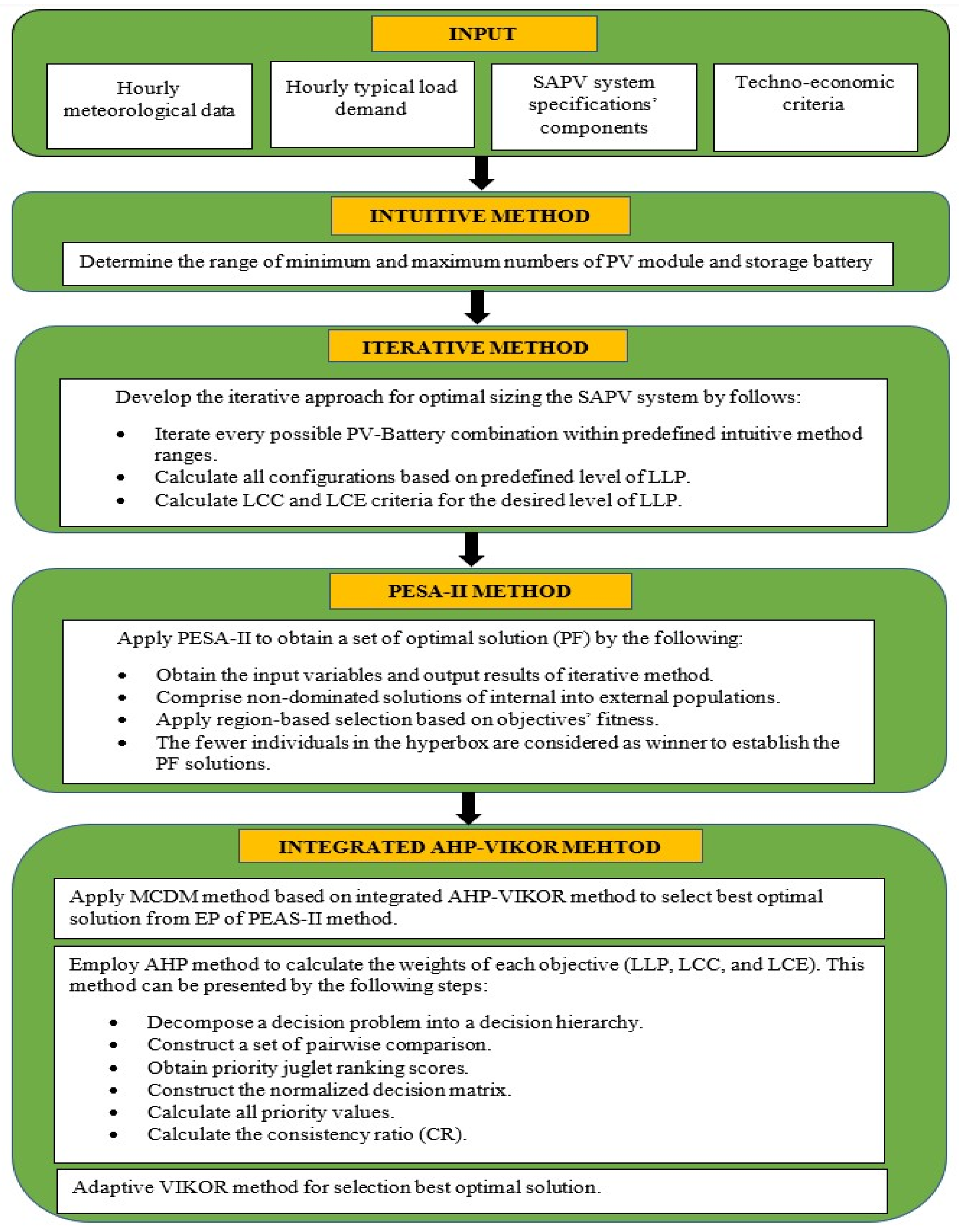
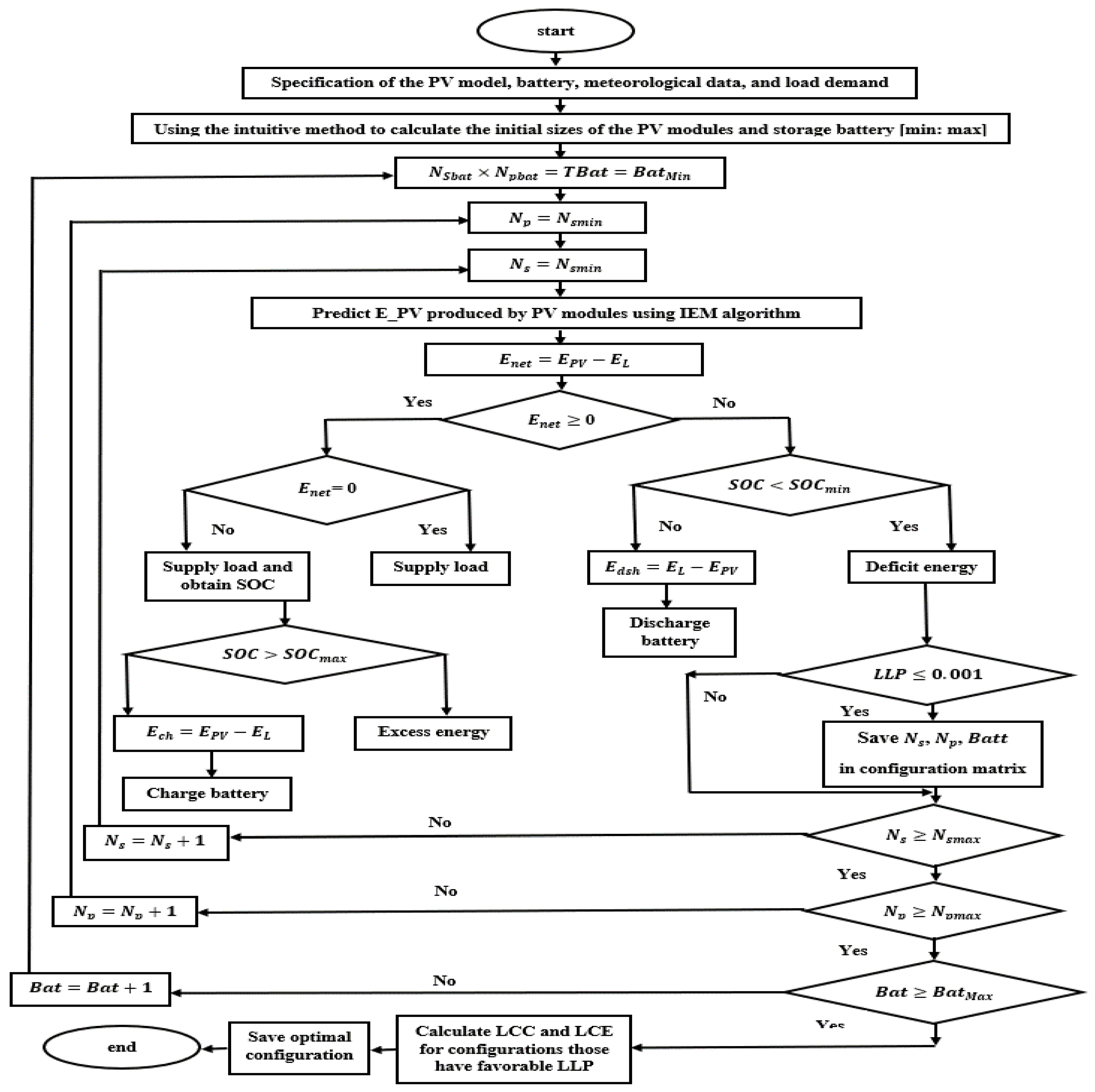
In this study, the proposed methodology was obtained in order to find a set of optimal configurations of the SAPV system to supply the load demand for a house in a remote area. Firstly, the intuitive method was employed to determine the search space of PV modules (series and parallel) and the three types of storage batteries (lead–acid, AGM, and lithium-ion). The ranges of the search space, which consisted of the number of PV modules and number of storage batteries used in the iterative method, were chosen by utilizing the intuitive method from 1 to 40 for series and parallel PV modules, whereas the range of the number of the storage battery was chosen from 3 to 50. The safety factor was set as 2 in the intuitive method. Afterward, the iterative method was used to construct sets of optimum configurations using a wide range of reliability and costs for the three types of storage batteries. The main advantage of the numerical approach is that the global optimal solutions can be reached by investigating all possible configurations in the design space. The numerical approach started by increasing $N_s$ and $N_p$ one by one in the first loop and the second loop, respectively. Meanwhile, the number of the storage battery increased in the third loop. Therefore, the numbers of configurations based on the numerical method were 59,503, 45,806, and 40,098 and the central processing unit (CPU) executions times were 10,295.71 s, 8151.07 s, and 8656.25 s for the lead–acid, AGM, and lithium-ion batteries, respectively. Figure 9 shows the correlation between the LLP, LCC, and LCE starting from the minimum value of each objective and ending at the maximum value by using the numerical approach for lead–acid, AGM, and lithium-ion storage batteries. According to [13], the acceptable level of LLP is equal to 1%. Thus, the favorable level of LLP was set at $\ge$0.1%. For convenience, the maximum and minimum values of LLP, LCC, and LCE objectives with their numbers of PV modules and storage batteries are tabulated in

Table 6. Minimum values and maximum values of loss of load probability (LLP), life cycle cost (LCC), and levelized cost of energy (LCE) were found by the numerical method for three types of storage batteries.

	N	Np	Ns	Bat	LLP	LCC	LCE	E_deficit	E_excess	Cost Year
Lead-acid	1	1	1	3	0.99361	6003.1637	43.5509	22,155.5077	0	300.1581	Max
	550	22	25	31	0.00100	96,867.2686	1.2777	22.3026	57,033.9955	4843.3634	Min
	1600	40	40	29	0.00134	255,066.1754	1.1565	30.0875	203,227.978	12,753.309	Max
	1	1	1	3	0.99361	6003.1637	43.5509	22,155.5077	0	300.15819	Min
	1	1	1	50	0.99145	19,188.8540	139.209	22,107.2725	0	959.4427	Max
	1600	40	40	3	0.36590	247,771.9637	1.1234	8158.9069	207,101.433	12,388.598	Min
AGM	1	1	1	3	0.99343	8141.6763	59.065	22,151.5118	0	407.0838	Max
	234	6	39	21	0.00100	61,252.1907	1.899	22.4923489	11,665.9793	3062.6095	Min
	1600	40	40	12	0.00103	258,850.9335	1.1737	23	203,227.978	12,942.547	Max
	1	1	1	3	0.99343	8141.6763	59.065	22,151.5118	0	407.0838	Min
	1	1	1	50	0.98965	68,474.6293	667.53	22,067.2335	0	3423.7315	Max
	1600	40	40	3	0.30697	249,910.4763	1.1331	6844.92315	206,702.985	12,495.524	Min
Lithium-ion	1	1	1	3	0.99308	44,169.0240	320.43	22,143.6177	0	2208.4512	Max
	247	13	19	41	0.00010	769,048.9375	30.353	2.33138135	3851.09968	38,452.447	Min
	242	11	22	50	0.00021	927,810.7404	37.375	4.77143466	3356.36454	46,390.537	Max
	1	1	1	3	0.99308	44,169.0240	320.43	22,143.6177	0	2208.4512	Min
	1	1	1	50	0.98362	891,371.5404	8689.5	21,932.6481	0	44,568.577	Max
	1600	40	40	3	0.15917	285,937.8241	1.2965	3549.24315	205,341.293	14,296.891	Min

.

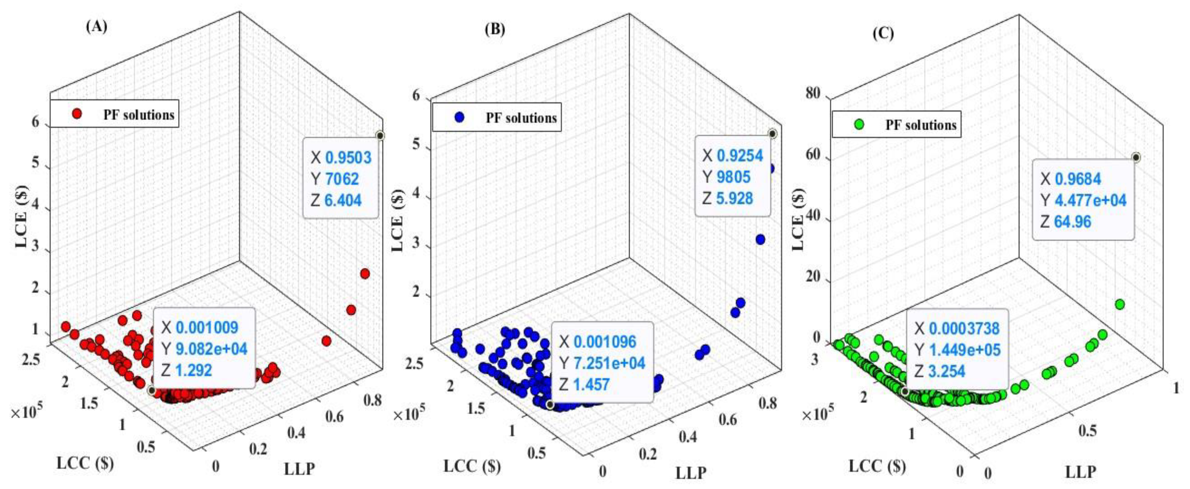
It is worth mentioning that selecting the optimal configuration from large numbers of configurations using the numerical method is a complex task. It is necessary to nominate a set of optimal solutions to be represented as optimal PF of multi-objectives by simultaneously minimizing the LLP, LCC, and LCE. On this basis, the PESA-II method was employed to perform this task. As mentioned in the literature, the difficulty of several multi-objective algorithms is in comparing two conflicting solutions and finding the fitness of the most probable solution. Moreover, the obtained PF must achieve three objectives, which are convergence, diversity, and coverage. In this research study, PSEA-II is used to obtain a set of optimal PF solutions based on three conflicting objectives, which are LLP, LCC, and LCE. The correlation between LLP, LCC, and LCE objectives using three types of batteries is illustrated in Figure 10. The aim of obtaining sets of PF solutions is to minimize the three objectives, and the trade-off is shown in Figure 10. From Figure 11, the PESA-II method can efficiently obtain sets of PF solutions for lead–acid, AGM, and lithium-ion batteries in terms of good spread, convergence, and coverage. The CPU execution time of the three sets PF solutions for the lead–acid, AGM, and lithium-ion batteries were 19,810.81 s, 4783.03 s, and 1347.06 s, respectively. For more convenience, the minimum and maximum values of the three objectives for the three types of batteries using the PESA-II method are tabulated in

Table 7. Minimum and maximum values of three objectives were found on the basis of the PESA-II method.

Battery Types	Lead–Acid			AGM			Lithium-Ion
Objective	LLP	LCC	LCE	LLP	LCC	LCE	LLP	LCC	LCE
Min	0.00100	7060.5640	1.1301	0.00109	8704.8760	1.1406	0.00037	44,773.8241	1.3181
Max	0.95034	247,334.8958	6.4037	0.92544	248,829.3970	5.9276	0.96838	286,995.5341	64.9638

.

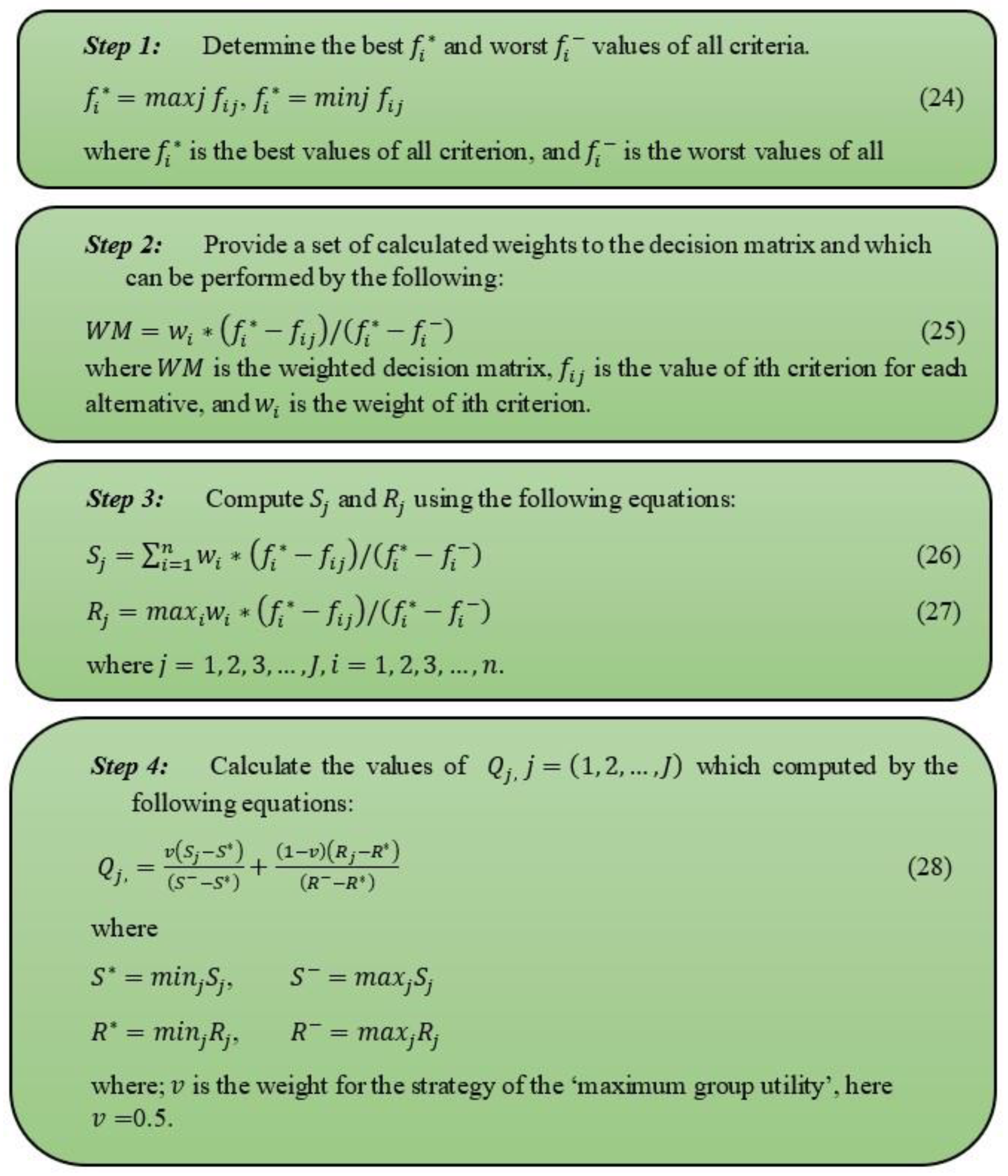
It is evident that the optimal PF solutions were efficiently constructed on the basis of the PESA-II method for three types of storage batteries. Therefore, the integrated AHP-VIKOR method was employed in order to arrange the preference of the optimal solutions. According to Table 4 and Table 5, the first evaluator gave extreme importance to LLP over LLC, and very strong importance to LCC over LCE. Meanwhile, equality was given between LCC and LCE. The second evaluator assumed equality between LLP and LCC, and very strong importance of LLP over LCE. Contrastingly, it gave extreme importance to LCC over LCE. The third evaluator proposed moderate and strong importance of LLP over LCC and LCE, respectively, whereas it gave moderate importance to LCC over LCE. Thus, values of weights for LLP, LCC, and LCE objectives were (0.79, 0.1, and 0.1) for the first evaluator, (0.48, 0.44, and 0.07) for the second evaluator, and (0.63, 0.26, and 0.1) for the third evaluator as illustrated in Table 5. The consistency ratios (CR) for the three evaluators were 0.006, 0.01, and 0.033. The minimum CR value was recommended and meant the values of the given weights to the three conflicting objectives were stable and perfectly consistent. The results of the AHP-VIKOR method based on three evaluators for the lead–acid battery are given in

Table 8. (A) Results of the AHP-VIKOR method of the SAPV system based on the lead–acid battery for the first evaluator. (B) Results of the AHP-VIKOR method of the SAPV system based on the lead–acid battery for the second evaluator. (C) Results of the AHP-VIKOR method of the SAPV system based on the lead–acid battery for the third evaluator.

(A)
Si	Ri	Qi	LLP	LCC	LCE	N	Ns	Np	Bat	Friedman Rank
0.0298	0.0207	0.0028	0.0036	56,884.91	1.4738	280	7	40	34	10
0.0307	0.0198	0.0027	0.0012	54,742.71	1.6686	238	34	7	49	9
0.0319	0.0185	0.0025	0.0048	51,547.43	1.6401	228	38	6	43	8
0.0317	0.0184	0.0024	0.0053	51,439.93	1.6154	231	21	11	41	7
0.0311	0.0190	0.0020	0.0031	52,713.32	1.6483	232	8	29	45	6
0.0293	0.0204	0.0020	0.0026	56,214.55	1.5104	270	9	30	37	5
0.0300	0.0197	0.0023	0.0027	54,615.13	1.5722	252	36	7	41	4
0.0294	0.0202	0.0023	0.0017	55,824.73	1.5576	260	13	20	41	3
0.0306	0.0191	0.0022	0.0040	52,973.79	1.5815	243	27	9	40	2
0.0301	0.0195	0.0022	0.0032	54,032.19	1.5679	250	25	10	40	1
(B)
Si	Ri	Qi	LLP	LCC	LCE	N	Ns	Np	Bat	Friedman Rank
0.0923	0.0836	0.0341	0.0031	52,713.32	1.6483	232	8	29	45	10
0.0909	0.0814	0.0302	0.0048	51,547.43	1.6401	228	38	6	43	9
0.0906	0.0812	0.0296	0.0053	51,439.93	1.6154	231	21	11	41	8
0.0903	0.0793	0.0273	0.0103	50,556.36	1.5282	240	8	30	33	7
0.1102	0.0583	0.0233	0.0886	38,915.74	1.6040	176	8	22	26	6
0.0879	0.0755	0.0201	0.0109	48,330.29	1.6232	216	24	9	38	5
0.0955	0.0679	0.0192	0.0431	44,185.88	1.5337	209	11	19	27	4
0.0880	0.0735	0.0180	0.0169	47,251.82	1.5581	220	10	22	32	3
0.0925	0.0643	0.0117	0.0427	42,176.58	1.5936	192	16	12	29	2
0.0889	0.0663	0.0103	0.0300	43,276.91	1.6524	190	10	19	34	1
(C)
Si	Ri	Qi	LLP	LCC	LCE	N	Ns	Np	Bat	Friedman Rank
0.0611	0.0508	0.0111	0.0032	54,032.19	1.5679	250	25	10	40	10
0.0751	0.0379	0.0106	0.0427	42,176.58	1.5936	192	16	12	29	9
0.0612	0.0494	0.0100	0.0031	52,713.32	1.6483	232	8	29	45	8
0.0608	0.0496	0.0099	0.0040	52,973.79	1.5815	243	27	9	40	7
0.0609	0.0481	0.0087	0.0048	51,547.43	1.6401	228	38	6	43	6
0.0606	0.0480	0.0084	0.0053	51,439.93	1.6154	231	21	11	41	5
0.0612	0.0470	0.0080	0.0103	50,556.36	1.5282	240	8	30	33	4
0.0690	0.0391	0.0071	0.0300	43,276.91	1.6524	190	10	19	34	3
0.0627	0.0434	0.0061	0.0169	47,251.82	1.5581	220	10	22	32	2
0.0611	0.0446	0.0059	0.0109	48,330.29	1.6232	216	24	9	38	1

A–C. The optimal configurations were ranked by the Qi value in descending order and Friedman rank for the first 10 to 200 configurations. The first optimal configuration of the SAPV system based on the lead–acid battery for the first evaluator was composed of 250 numbers of PV modules (25 in series and 10 in parallel) and 40 numbers of storage batteries at an LLP equal to 0.00324, as well as the values of LCC and LCE being USD 54,032.19 and USD 1.5679, respectively. The Qi value decreased from 1 to 0.0022 at the first rank from 200 configurations on the basis of the Friedman rank. The CPU execution for the first evaluator was 0.656 s. Meanwhile, the first optimal configuration for the second evaluator based on the lead–acid battery consisted of 190 PV modules (10 in series and 19 in parallel) and 34 storage batteries at 0.03 LLP, and the values of LCC and LCE were $43,276.91 and $1.6524, respectively. The value of Qi at first rank was 0.0103 from 200 solutions using the Friedman rank. The CPU execution time was 0.4062 s. The results of optimal configurations of the third evaluator using the lead–acid battery were given by 216 PV modules (24 in series and 9 in parallel) and 38 storage batteries at LLP equal to 0.0109, and the values of LCC and LCE were $48,330.29 and $1.6232, respectively. The Qi value was 0.0059 at first rank of 200 configurations on the basis of the Friedman rank method. The CPU execution of the third evaluator for the lead–acid battery was 0.5156 s. The results of the AHP-VIKOR method based on the laid battery for three evaluators can be found in Table 8A–C. It can be observed that the value of Qi was largely dependent on the given weight values by the evaluators for the three objectives. Moreover, the solution gained with min Si is a maximum group utility and the solution gained Ri is with a minimum individual of regret of the “opponent”. Thus, it had a proportional relationship with Si and Ri. The minimum value of Qi was registered in the first evaluator at 0.0022, then followed by third and second evaluators. This confirms that each configuration was ranked according to the weight values. The PESA-II method showed its ability to achieve a trade-off between LLP, LCC, and LCE objectives. This fact can be seen in the values of Qi within the first 10 configurations of rank, as shown in Table 8A–C. In Table 8B, the values of LLP were reduced from 0.03 at 1st rank to 0.003 at 10th rank, and the LCC values were increased from $43,276.91 to $52,713.91. The LCE values were changed on the basis of the energy conducted by the PV modules and the capacity of the storage batteries during the period of time.

In a similar manner to

Table 9. (A) Results of the AHP-VIKOR method of the SAPV system based on the AGM battery for the first evaluator. (B) Results of the AHP-VIKOR method of the SAPV system based on the AGM battery for the second evaluator. (C) Results of the AHP-VIKOR method of the SAPV system based on AGM battery for the third evaluator.

(A)
Si	Ri	Qi	LLP	LCC	LCE	N	Ns	Np	Bat	Friedman Rank
0.0350	0.0229	0.0039	0.0063	64,558.93	1.4868	315	21	15	12	10
0.0352	0.0212	0.0030	0.0015	60,691.24	1.7611	250	25	10	18	9
0.0346	0.0211	0.0026	0.0019	60,453.85	1.7198	255	15	17	17	8
0.0329	0.0226	0.0025	0.0033	63,889.12	1.5246	304	38	8	13	7
0.0365	0.0193	0.0025	0.0090	56,026.72	1.6129	252	18	14	13	6
0.0321	0.0230	0.0023	0.0012	64,882.5	1.5483	304	16	19	14	5
0.0338	0.0214	0.0023	0.0020	61,123.67	1.6670	266	14	19	16	4
0.0327	0.0219	0.0020	0.0026	62,160.9	1.5767	286	22	13	14	3
0.0338	0.0209	0.0019	0.0032	59,827.89	1.6440	264	22	12	15	2
0.0335	0.0210	0.0019	0.0039	60,195.3	1.5996	273	13	21	14	1
(B)
Si	Ri	Qi	LLP	LCC	LCE	N	Ns	Np	Bat	Friedman Rank
0.1031	0.0932	0.0461	0.0019	60,453.85	1.7198	255	15	17	17	10
0.1017	0.0927	0.0440	0.0039	60,195.3	1.5996	273	13	21	14	9
0.1014	0.0920	0.0429	0.0032	59,827.89	1.6440	264	22	12	15	8
0.1306	0.0644	0.0414	0.1131	44,795.58	1.5930	204	6	34	9	7
0.1291	0.0638	0.0391	0.1224	39,892.17	1.7539	165	5	33	10	6
0.1012	0.0817	0.0305	0.0253	54,191.15	1.5539	253	11	23	11	5
0.0969	0.0850	0.0299	0.0090	56,026.72	1.6129	252	18	14	13	4
0.1185	0.0620	0.0257	0.0920	43,520.97	1.6705	189	21	9	10	3
0.0943	0.0710	0.0105	0.0249	48,401.7	1.8007	195	5	39	14	2
0.1012	0.0637	0.0094	0.0528	44,449.33	1.7717	182	14	13	12	1
(C)
Si	Ri	Qi	LLP	LCC	LCE	N	Ns	Np	Bat	Friedman Rank
0.0676	0.0569	0.0172	0.0026	62,160.90	1.576771	286	22	13	14	10
0.0693	0.0553	0.0172	0.0015	60,691.24	1.761179	250	25	10	18	9
0.0681	0.0558	0.0167	0.0020	61,123.67	1.667037	266	14	19	16	8
0.0685	0.0550	0.0163	0.0019	60,453.85	1.719892	255	15	17	17	7
0.0871	0.0376	0.0155	0.0528	44,449.33	1.771786	182	14	13	12	6
0.0669	0.0548	0.0149	0.0039	60,195.3	1.599622	273	13	21	14	5
0.0740	0.0482	0.0147	0.0253	54,191.15	1.553908	253	11	23	11	4
0.0670	0.0544	0.0146	0.0032	59,827.89	1.644058	264	22	12	15	3
0.0661	0.0502	0.0105	0.0090	56,026.72	1.612917	252	18	14	13	2
0.0729	0.0419	0.0086	0.0249	48,401.7	1.800709	195	5	39	14	1

and

Table 10. (A) Results of the AHP-VIKOR method of the SAPV system based on the lithium-ion battery for the first evaluator. (B) Results of the AHP-VIKOR method of the SAPV system based on the lithium-ion battery for the second evaluator. (C) Results of the AHP-VIKOR method of the SAPV system based on the lithium-ion battery for the third evaluator.

(A)
Si	Ri	Qi	LLP	LCC	LCE	N	Ns	Np	Bat	Friedman Rank
0.0417	0.0370	0.0057	0.0030	134,433.3	2.8684	340	10	34	6	10
0.0501	0.0295	0.0057	0.0203	116,289.3	3.8347	220	11	20	6	9
0.0490	0.0297	0.0052	0.0187	116,894.1	3.7858	224	8	28	6	8
0.0413	0.0357	0.0046	0.0039	131,258.1	2.9850	319	29	11	6	7
0.0414	0.0347	0.0041	0.0050	128,990.1	3.0782	304	38	8	6	4.5
0.0414	0.0347	0.0041	0.0050	128,990.1	3.0782	304	19	16	6	4.5
0.0414	0.0347	0.0041	0.0050	128,990.1	3.0782	304	16	19	6	4.5
0.0414	0.0347	0.0041	0.0050	128,990.1	3.0782	304	8	38	6	4.5
0.0451	0.0312	0.0039	0.0129	120,371.7	3.5354	247	19	13	6	2
0.0430	0.0329	0.0038	0.0086	124,605.3	3.2871	275	11	25	6	1
(B)
Si	Ri	Qi	LLP	LCC	LCE	N	Ns	Np	Bat	Friedman Rank
0.1549	0.0900	0.0388	0.1259	94,366.72	2.7716	247	13	19	4	10
0.1365	0.1073	0.0385	0.0535	103,891.6	3.3647	224	28	8	5	9
0.1365	0.1062	0.0371	0.0555	103,286.8	3.4059	220	11	20	5	8
0.1572	0.0861	0.0369	0.1719	82,421.92	3.5591	168	8	21	4	7
0.1498	0.0920	0.0353	0.1087	95,424.42	4.1206	168	6	28	5	6
0.1562	0.0846	0.0338	0.1689	82,724.32	3.5302	170	10	17	4	5
0.1365	0.1032	0.0335	0.0613	101,623.6	3.5274	209	19	11	5	4
0.1531	0.0837	0.0290	0.1345	90,889.12	2.9436	224	7	32	4	3
0.1523	0.0771	0.0202	0.1456	87,260.32	3.1652	200	25	8	4	2
0.1520	0.0758	0.0181	0.1476	86,504.32	3.2182	195	39	5	4	1
(C)
Si	Ri	Qi	LLP	LCC	LCE	N	Ns	Np	Bat	Friedman Rank
0.0990	0.0725	0.0147	0.0368	112,358.8	2.9111	280	10	28	5	10
0.0935	0.0774	0.0147	0.0187	116,894.1	3.7858	224	8	28	6	9
0.0940	0.0767	0.0145	0.0203	116,289.3	3.8347	220	11	20	6	8
0.0966	0.0741	0.0143	0.0278	113,870.1	4.0494	204	34	6	6	7
0.0955	0.0751	0.0143	0.0249	114,777.3	3.9651	210	10	21	6	6
0.0998	0.0665	0.0100	0.0464	106,764.4	3.1874	243	9	27	5	5
0.1007	0.0645	0.0091	0.0506	104,950	3.2960	231	21	11	5	4
0.1045	0.0610	0.0089	0.0613	101,623.6	3.5274	209	19	11	5	3
0.1023	0.0628	0.0087	0.0555	103,286.8	3.4059	220	11	20	5	2
0.1016	0.0634	0.0087	0.0535	103,891.6	3.3647	224	28	8	5	1

, the Qi values had minimum values with the first evaluator at a high level of accuracy according to the given weight value to LLP. The Qi values at 1^st rank for the first evaluator for the AGM and lithium-ion storage batteries were 0.0019 and 0.0038, respectively. Meanwhile, the Qi values at the first rank for the second and third evaluators based on AGM and lithium-ion batteries were 0.0094, 0.0086, 0.0181, and 0.0087, respectively. From Table 10 (part A), it can be noted that there were four configurations with the rank of 4.5; this happened due to interdependence in total numbers of PV modules and storage batteries. The configurations in Table 10, some configurations of Table 9, and some configurations in Table 8 (part B) had undesirable levels of LLP. This was because the second evaluator gave moderate importance between LLP and LCC objectives, as observed from Qi values that were larger than others. Therefore, a higher priority must be given to the LLP objective in designing of SAPV system. The CPU_execution times for the three evaluators based on AGM and lithium-ion storage batteries were 0.5468, 0.4531, 0.6093, 0.5781, 0.3437, and 0.4218 s. It was clear that the computational times of the three evaluators based on the lithium-ion battery were less than AGM and lead–acid. This was because of the large capacity of the lithium-ion battery, which is about 6.6 kWh compared with other batteries. However, the lithium-ion battery is very expensive compared with AGM and lead–acid batteries at the same level of reliability, as illustrated in Table 8, Table 9 and Table 10 (part A). Moreover, the levelized cost of energy values presented by the lead–acid battery were less than other batteries, which makes the lead–acid battery more suitable in the designing of a SAPV system. However, more replacement times in the lead–acid battery are required. In this regard, it is prudent to choose the lead–acid battery for the three evaluators at first rank to analyze the performance of the SAPV system for one year.

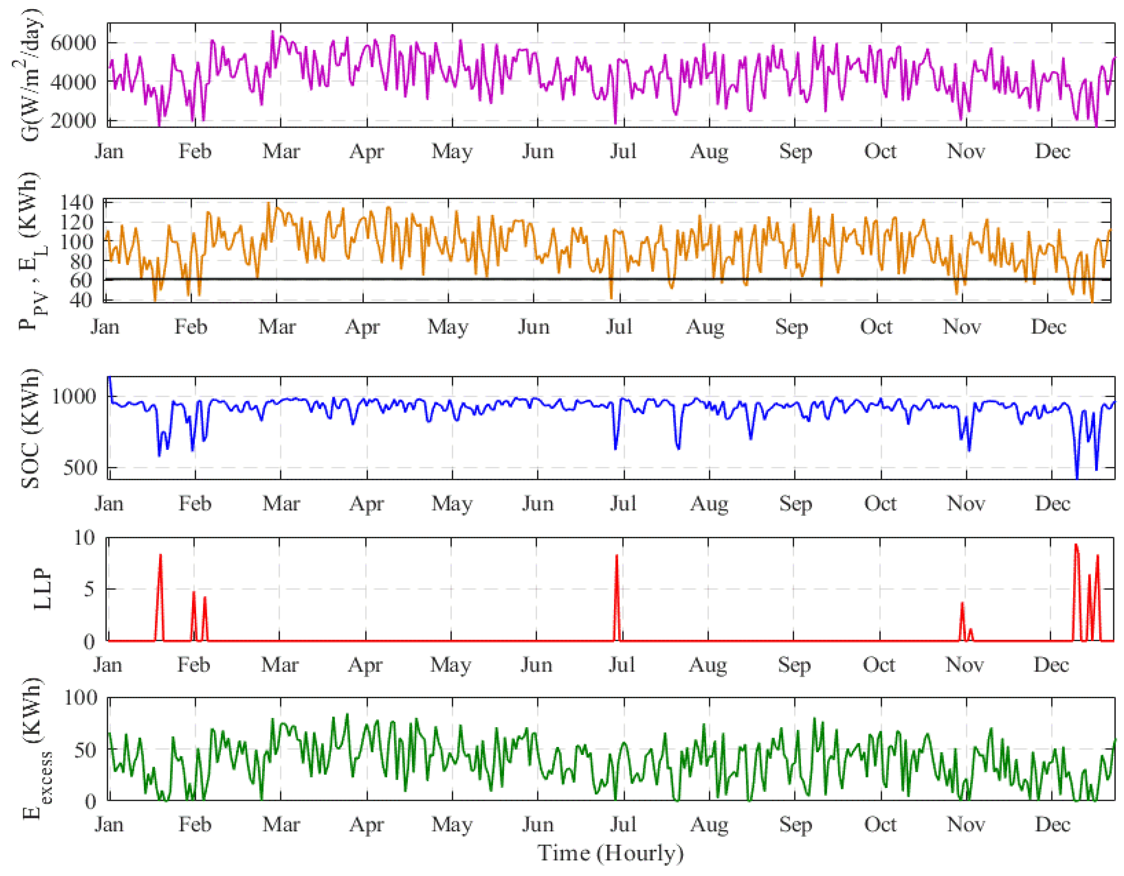
The daily performance of the SAPV system under the optimal configuration, which was composed of 250 PV modules (25 in series and 10 in parallel) and 40 lead-acid storage batteries, is illustrated in Figure 12. The first subplot shows solar irradiation (G) using hourly meteorological data for one year. Meanwhile, the output power of PV modules (P_PV) and load demand (E_L) are illustrated in the second subplot; the average G and P_PV over one year were around 4363.8 Wh/m²/day and 2938.4 KWh, respectively. The state of charge (SOC), deficit energy (E_deficit), and dumped energy (E_dump) are shown in the third, fourth, and fifth subplots, respectively. According to Figure 12, the SAPV system was usually able to fulfill the required load demand through the year, except for 12 days, as demonstrated in

Table 11. Performance data of SAPV system during shortage of days.

Sequence no.	Date	G (W/m2)	P_PV (KWh)	SOC (KWh)	E_deficit (KWh)
1	19 January	1658.4	37.8	572.2	4.5
2	20 January	3802.8	83.5	764.1	8.3
3	01 February	3968.8	68.9	774.8	4.7
4	05 February	3841.6	86.9	711.6	4.2
5	07 July	5138.9	111.8	756	8.3
6	06 November	3975	87.5	754	3.7
7	09 November	4179.2	91.8	783.3	1.2
8	17 December	1969.5	44.6	407	9.3
9	18 December	3330.5	73.2	730.4	8.5
10	22 December	3966.5	86.6	738.7	6.4
11	24 December	1591.7	36	471.8	4.5
12	25 December	4174.8	91.2	734.5	8.3

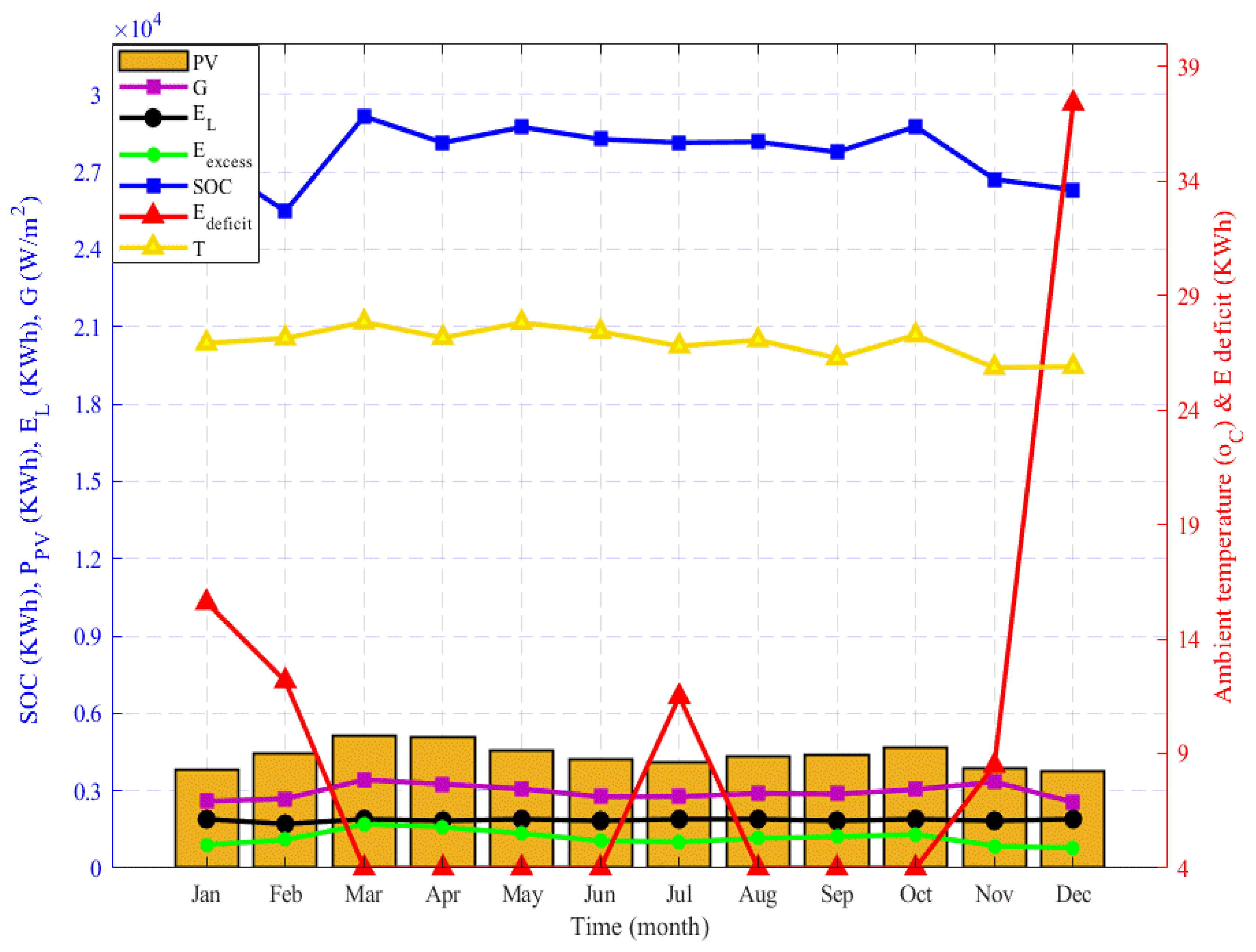
. The deficit energy for one year was about 72 kWh/year, which is equal to 28 h under the chosen optimal configuration at 0.0032 LLP. In the third subplot, the SOC was almost at high levels, except for the days listed in Table 11. The reason for this is that level of solar irradiance is low, especially in December, as shown in the fourth subplot. The last subplot indicated excess energy for one year. From Table 11, the lowest average daily solar irradiance was registered on 24 December at about 1591.7 Wh/m²/day. Therefore, the output power of PV modules, SOC, and deficit energy were 36 KWh, 471.8 KWh, and 4.5 KWh, respectively. In fact, the shortages almost happened in the early morning before the appearance of sunshine due to the low solar irradiance before one day, and the amount of energy stored in batteries was very little. On the other hand, the maximum solar irradiance occurred on 1 March and was about 6638.8 Wh/m²/day. Thus, the output power of PV modules, SOC, and excess energy were 140 KWh, 975 KWh, and 79.6 KWh, respectively.

Figure 13 shows the monthly state of charge, the output power of PV modules, load demand, excess energy, deficit energy, and ambient temperature for one year. As stated previously, the maximum solar irradiance occurred in March, whereas the minimum solar irradiance was registered in December, as illustrated in Figure 13.

Last but not least, several observations were noted, as follows:

• Employing the intuitive method can significantly reduce the computational time of the iterative approach, which was found to be very accurate compared with other methods.
• The PESA-II method demonstrated its capability not only in obtaining PF solutions considering three conflicting objectives, but also by reducing the big solutions in the design space using binary tournament selection.
• An effective and integrated AHP-VIKOR method allowed for the reaching of the final optimum configuration and selected the most appropriate storage battery for the SAPV system.
• The performance of the proposed SAPV system was analyzed on the basis of hourly metrological data for one year.
• Overall, our proposed novel iterative-hybrid method tended to be very accurate compared with metaheuristic multi-objective optimization methods due to its random nature, which led to the omission of several important solutions.

It is worth mentioning that there were some limitations that should be considered in future work, such as selecting optimal configurations on the basis of PESA-II to establish set PF solutions, which can be improved by using another method that has a better capacity to deal with large data conducted by a numerical method. Moreover, the given weights’ values by using AHP method can be improved because the AHP method requires manual calculations.

7. Conclusions

This paper presented a novel approach by integrating iterative-PESA-II and AHP-VIKOR methods to find an optimum configuration of the SAPV system on the basis of techno-economic criteria and in considering various types of storage battery. The results demonstrated that the desirable and most suitable configuration for the SAPV system was chosen according to the first expert based on lead–acid battery, which consisted of 250 PV modules (25 in series and 10 in parallel) and 40 storage batteries. The values of Qi, LLP, LCC, and LCE of the optimum configuration were 0.0022, 0.0032, 54032.19, and 1.56 USD, respectively. Therefore, the performance analysis study based on the most favorable configuration was also presented for one year. The optimal configuration of the SAPV system consisted of 872 PV modules and 28 storage batteries. The proposed new hybrid method showed high accuracy in finding the optimal configuration compared with meta-heuristic and numerical methods. The proposed hybrid method showed that the SAPV system could not meet the required load demand only 28 h of one year, which is a promising method to tackle optimization problems.

References

1. Khalilpour, R.; Vassallo, A. Leaving the grid: An ambition or a real choice? Energy Policy 2015, 82, 207–221. [Google Scholar] [CrossRef]
2. Alsadi, S.; Khatib, T. Photovoltaic power systems optimization research status: A review of criteria, constrains, models, techniques, and software tools. Appl. Sci. 2018, 8, 1761. [Google Scholar] [CrossRef] [Green Version]
3. Al-Falahi, M.D.A.; Jayasinghe, S.D.G.; Enshaei, H. A review on recent size optimization methodologies for standalone solar and wind hybrid renewable energy system. Energy Convers. Manag. 2017, 143, 252–274. [Google Scholar] [CrossRef]
4. Goel, S.; Sharma, R. Performance evaluation of stand alone, grid connected and hybrid renewable energy systems for rural application: A comparative review. Renew. Sustain. Energy Rev. 2017, 78, 1378–1389. [Google Scholar] [CrossRef]
5. Khatib, T.; Elmenreich, W. Modeling of Photovoltaic Systems Using Matlab; John Wiley & Sons, Inc.: Hoboken, NJ, USA, 2016; Available online: https://books.google.ca/books?id=Wd9QDAAAQBAJ (accessed on 22 August 2019).
6. Vázquez, M.J.V.; Márquez, J.M.A.; Manzano, F.S. A methodology for optimizing stand-alone PV-system size using parallel-connected DC/DC converters. IEEE Trans. Ind. Electron. 2008, 55, 2664–2673. [Google Scholar] [CrossRef]
7. Krieger, E.M.; Cannarella, J.; Arnold, C.B. A comparison of lead-acid and lithium-based battery behavior and capacity fade in off-grid renewable charging applications. Energy 2013, 60, 492–500. [Google Scholar] [CrossRef]
8. Benavente, F.; Lundblad, A.; Campana, P.E.; Zhang, Y.; Cabrera, S.; Lindbergh, G. Photovoltaic/battery system sizing for rural electrification in Bolivia: Considering the suppressed demand effect. Appl. Energy 2019, 235, 519–528. [Google Scholar] [CrossRef]
9. Mandelli, S.; Barbieri, J.; Mereu, R.; Colombo, E. Off-grid systems for rural electrification in developing countries: Definitions, classification and a comprehensive literature review. Renew. Sustain. Energy Rev. 2016, 58, 1621–1646. [Google Scholar] [CrossRef]
10. Khatib, T.; Ibrahim, I.A.; Mohamed, A. A review on sizing methodologies of photovoltaic array and storage battery in a standalone photovoltaic system. Energy Convers. Manag. 2016, 120, 430–448. [Google Scholar] [CrossRef]
11. Khatib, T.; Mohamed, A.; Sopian, K. A review of photovoltaic systems size optimization techniques. Renew. Sustain. Energy Rev. 2013, 22, 454–465. [Google Scholar] [CrossRef]
12. Kumar, A.; Singh, A.R.; Deng, Y.; He, X.; Kumar, P.; Bansal, R.C. A novel methodological framework for the design of sustainable rural microgrid for developing nations. IEEE Access 2018, 6, 24925–24951. [Google Scholar] [CrossRef]
13. Kazem, H.A.; Khatib, T.; Sopian, K. Sizing of a standalone photovoltaic/battery system at minimum cost for remote housing electrification in Sohar, Oman. Energy Build. 2013, 61, 108–115. [Google Scholar] [CrossRef]
14. Khatib, T.; Sopian, K.; Kazem, H.A. Actual performance and characteristic of a grid connected photovoltaic power system in the tropics: A short term evaluation. Energy Convers. Manag. 2013, 71, 115–119. [Google Scholar] [CrossRef]
15. Ibrahim, I.A.; Khatib, T.; Mohamed, A. Optimal sizing of a standalone photovoltaic system for remote housing electrification using numerical algorithm and improved system models. Energy 2017, 126, 392–403. [Google Scholar] [CrossRef]
16. Spertino, F.; di Leo, P.; Cocina, V.; Tina, G.M. Storage sizing procedure and experimental verification of stand-alone photovoltaic systems. In Proceedings of the 2012 IEEE International Energy Conference and Exhibition (ENERGYCON), Florence, Italy, 9–12 September 2012; pp. 464–468. [Google Scholar] [CrossRef]
17. Semaoui, S.; Arab, A.H.; Bacha, S.; Azoui, B. Optimal sizing of a stand-alone photovoltaic system with energy management in isolated areas. Energy Procedia 2013, 36, 358–368. [Google Scholar] [CrossRef] [Green Version]
18. Okoye, C.O.; Solyalı, O. Optimal sizing of stand-alone photovoltaic systems in residential buildings. Energy 2017, 126, 573–584. [Google Scholar] [CrossRef]
19. Ayop, R.; Isa, N.M.; Tan, C.W. Components sizing of photovoltaic stand-alone system based on loss of power supply probability. Renew. Sustain. Energy Rev. 2018, 81, 2731–2743. [Google Scholar] [CrossRef]
20. Deb, K.; Member, A.; Pratap, A.; Agarwal, S.; Meyarivan, T. A fast and elitist multiobjective genetic algorithm: NSGA-II. IEEE Trans. Evol. Comput. 2002, 6, 182–197. [Google Scholar] [CrossRef] [Green Version]
21. Knowles, J.; Corne, D. The Pareto archived evolution strategy: A new baseline algorithm for Pareto multiobjective optimization. In Proceedings of the 1999 Congress on Evolutionary Computation-CEC99 (Cat. No. 99TH8406), Washington, DC, USA, 6–9 July 1999; Volume 1, pp. 98–105. [Google Scholar] [CrossRef]
22. Zitzler, E.; Laumanns, M.; Thiele, L. SPEA2: Improving the strength pareto evolutionary algorithm. Evol. Methods Des. Optim. Control Appl. Ind. Probl. 2001, 236, 95–100. [Google Scholar]
23. Corne, D.; Jerram, N.; Knowles, J.; Oates, M.; Martin, J. PESA-II: Region-based selection in evolutionary multiobjective optimization. In Proceedings of the 3rd Annual Conference on Genetic and Evolutionary Computation, San Francisco, CA, USA, 7–11 July 2001; pp. 283–290. Available online: http://citeseerx.ist.psu.edu/viewdoc/summary?doi=10.1.1.10.2194 (accessed on 13 October 2019).
24. Dutta, S.; Das, K.N. A survey on pareto-based eas to solve multi-objective optimization problems. In Soft Computing for Problem Solving; Bansal, J., Das, K., Nagar, A., Deep, K., Ojha, A., Eds.; Advances in Intelligent Systems and Computing; Springer: Singapore, 2019. [Google Scholar] [CrossRef]
25. Tian, Y.; Cheng, R.; Zhang, X.; Jin, Y. PlatEMO: A MATLAB Platform for Evolutionary Multi-Objective Optimization [Educational Forum]. IEEE Comput. Intell. Mag. 2017, 12, 73–87. [Google Scholar] [CrossRef] [Green Version]
26. Lee, H.C.; Chang, C.T. Comparative analysis of MCDM methods for ranking renewable energy sources in Taiwan. Renew. Sustain. Energy Rev. 2018, 92, 883–896. [Google Scholar] [CrossRef]
27. Chel, A.; Tiwari, G.N.; Chandra, A. Simplified method of sizing and life cycle cost assessment of building integrated photovoltaic system. Energy Build. 2009, 41, 1172–1180. [Google Scholar] [CrossRef]
28. Rahman, M.; Islam, A.K.M.S.; Salehin, S.; Al-matin, M.A. Development of a Model for techno-economic assessment of a stand-alone off-grid solar photovoltaic system in bangladesh. Int. J. Renew. Energy Res. 2016, 6, 140–149. [Google Scholar]
29. Ghafoor, A.; Munir, A. Design and economics analysis of an off-grid PV system for household electri fi cation. Renew. Sustain. Energy Rev. 2015, 42, 496–502. [Google Scholar] [CrossRef]
30. Jakhrani, A.Q.; Othman, A.K.; Rigit, A.R.H.; Samo, S.R.; Kamboh, S.A. A novel analytical model for optimal sizing of standalone photovoltaic systems. Energy 2012, 46, 675–682. [Google Scholar] [CrossRef]
31. Dufo-López, R.; Lujano-Rojas, J.M.; Bernal-Agustín, J.L. Comparison of different lead-acid battery lifetime prediction models for use in simulation of stand-alone photovoltaic systems. Appl. Energy 2014, 115, 242–253. [Google Scholar] [CrossRef]
32. Huang, B.J.; Hou, T.F.; Hsu, P.-C.; Lin, T.H.; Chen, Y.T.; Chen, C.W.; Li, K.; Lee, K.Y. Design of direct solar PV driven air conditioner. Renew. Energy 2016, 88, 95–101. [Google Scholar] [CrossRef]
33. Khatib, T.; Mohamed, A.; Sopian, K.; Mahmoud, M. A new approach for optimal sizing of standalone photovoltaic systems. Int. J. Photoenergy 2012, 2012, 391213. [Google Scholar] [CrossRef]
34. Riza, D.F.A.L.; Gilani, S.I.U.H.; Aris, M.S. Standalone photovoltaic systems sizing optimization using design space approach: Case study for residential lighting load. J. Eng. Sci. Technol. 2015, 10, 943–957. [Google Scholar]
35. Perea-Moreno, A.J.; Hernandez-Escobedo, Q.; Garrido, J.; Verdugo-Diaz, J.D. Stand-alone photovoltaic system assessment in warmer urban areas in Mexico. Energies 2018, 11, 284. [Google Scholar] [CrossRef] [Green Version]
36. Nordin, N.D.; Rahman, H.A. A novel optimization method for designing stand alone photovoltaic system. Renew. Energy 2016, 89, 706–715. [Google Scholar] [CrossRef]
37. Mandelli, S.; Brivio, C.; Colombo, E.; Merlo, M. A sizing methodology based on levelized cost of supplied and lost energy for off-grid rural electrification systems. Renew. Energy 2016, 89, 475–488. [Google Scholar] [CrossRef] [Green Version]
38. Sarhan, A.; Hizam, H.; Mariun, N.; Ya’acob, M.E. An improved numerical optimization algorithm for sizing and configuration of standalone photo-voltaic system components in Yemen. Renew. Energy 2019, 134, 1434–1446. [Google Scholar] [CrossRef]
39. Bataineh, K.; Dalalah, D. Optimal Configuration for Design of Stand-Alone PV System. Smart Grid Renew. Energy 2012, 2012, 139–147. [Google Scholar] [CrossRef] [Green Version]
40. Sadio, A.; Fall, I.; Mbodji, S. New numerical sizing approach of a standalone photovoltaic power at Ngoundiane, Senegal. EAI Endorsed Trans. Energy Web 2018, 5, 1–12. [Google Scholar] [CrossRef] [Green Version]
41. Mohamed, A.F.; Elarini, M.M.; Othman, A.M. A new technique based on artificial bee colony algorithm for optimal sizing of stand-alone photovoltaic system. J. Adv. Res. 2013, 5, 397–408. [Google Scholar] [CrossRef] [Green Version]
42. Makhloufi, S. Comparative study between classical methods and genetic algorithms for sizing remote PV systems. Int. J. Energy Environ. Eng. 2015, 6, 221–231. [Google Scholar] [CrossRef] [Green Version]
43. Hlal, M.I.; Ramachandaramurthy, V.K.; Sarhan, A.; Pouryekta, A.; Subramaniam, U. Optimum battery depth of discharge for off-grid solar PV/battery system. J. Energy Storage 2019, 26, 100999. [Google Scholar] [CrossRef]
44. Khatib, T.; Elmenreich, W. An improved method for sizing standalone photovoltaic systems using generalized regression neural network. Int. J. Photoenergy 2014, 2014, 748142. [Google Scholar] [CrossRef]
45. Izzati, N.; Aziz, A.; Irwan, S.; Shaari, S.; Musirin, I.; Sopian, K. Optimal sizing of stand-alone photovoltaic system by minimizing the loss of power supply probability. Sol. Energy 2017, 150, 220–228. [Google Scholar] [CrossRef]
46. Ridha, H.M.; Gomes, C.; Hizam, H.; Ahmadipour, M. Optimal design of standalone photovoltaic system based on multi-objective particle swarm optimization: A case study of malaysia. Processes 2020, 8, 41. [Google Scholar] [CrossRef] [Green Version]
47. Habib, A.H.; Disfani, V.R.; Kleissl, J.; de Callafon, R.A. Optimal switchable load sizing and scheduling for standalone renewable energy systems. Sol. Energy. 2017, 144, 707–720. [Google Scholar] [CrossRef] [Green Version]
48. Esfahani, I.J.; Yoo, C. An optimization algorithm-based pinch analysis and GA for an off-grid batteryless photovoltaic-powered reverse osmosis desalination system. Renew. Energy 2016, 91, 233–248. [Google Scholar] [CrossRef]
49. Khatib, T.; Elmenreich, W. Novel simplified hourly energy flow models for photovoltaic power systems. Energy Convers. Manag. 2014, 79, 441–448. [Google Scholar] [CrossRef]
50. Ridha, H.M.; Gomes, C.; Hizam, H.; Mirjalili, S. Multiple Scenarios Multi-objective Salp Swarm Optimization for Sizing of Standalone Photovoltaic System. Renew. Energy. 2020. [Google Scholar] [CrossRef]
51. Kumar, A.; Sah, B.; Singh, A.R.; Deng, Y.; He, X.; Kumar, P.; Bansal, R.C. A review of multi criteria decision making (MCDM) towards sustainable renewable energy development. Renew. Sustain. Energy Rev. 2017, 69, 596–609. [Google Scholar] [CrossRef]
52. Jing, R.; Wang, M.; Zhang, Z.; Liu, J.; Liang, H.; Meng, C.; Shah, N. Energy & Buildings Comparative study of posteriori decision-making methods when designing building integrated energy systems with multi-objectives. Energy Build. 2019, 194, 123–139. [Google Scholar] [CrossRef]
53. Muhsen, D.H.; Nabil, M.; Haider, H.T.; Khatib, T. A novel method for sizing of standalone photovoltaic system using multi-objective differential evolution algorithm and hybrid multi-criteria decision making methods. Energy 2019. [Google Scholar] [CrossRef]
54. Opricovic, S.; Tzeng, G.H. Compromise solution by MCDM methods: A comparative analysis of VIKOR and TOPSIS. Eur. J. Oper. Res. 2004, 156, 445–455. [Google Scholar] [CrossRef]
55. Mardani, A.; Zavadskas, E.K.; Govindan, K. VIKOR technique: A systematic review of the state of the art literature on methodologies and applications. Sustain. Rev. 2016, 8, 37. [Google Scholar] [CrossRef] [Green Version]
56. Lupangu, C.; Bansal, R.C. A review of technical issues on the development of solar photovoltaic systems. Renew. Sustain. Energy Rev. 2017, 73, 950–965. [Google Scholar] [CrossRef]
57. Ridha, H.M.; Gomes, C.; Hizam, H. Estimation of photovoltaic module model’s parameters using an improved electromagnetic-like algorithm. Neural Comput. Appl. 2020. [Google Scholar] [CrossRef]
58. Ismail, M.S.; Moghavvemi, M.; Mahlia, T.M.I. Techno-economic analysis of an optimized photovoltaic and diesel generator hybrid power system for remote houses in a tropical climate. Energy Convers. Manag. 2013, 69, 163–173. [Google Scholar] [CrossRef]
59. Wang, R.; Li, G.; Ming, M.; Wu, G.; Wang, L. An efficient multi-objective model and algorithm for sizing a stand-alone hybrid renewable energy system. Energy 2017, 141, 2288–2299. [Google Scholar] [CrossRef]
60. Sidrach-De-Cardona, M.; López, L.M. A general multivariate qualitative model for sizing stand-alone photovoltaic systems. Sol. Energy Mater. Sol. Cells 1999, 59, 185–197. [Google Scholar] [CrossRef]
61. Muhsen, D.H.; Ghazali, A.B.; Khatib, T. Multiobjective differential evolution algorithm-based sizing of a standalone photovoltaic water pumping system. Energy Convers. Manag. 2016, 118, 32–43. [Google Scholar] [CrossRef]
62. Groumpos, P.P.; Papageorgiou, G. An optimal sizing method for stand-alone photovoltaic power systems. Sol. Energy 1987, 38, 341–351. [Google Scholar] [CrossRef]
63. Wholesale Solar, (n.d.). Available online: https://www.wholesalesolar.com/deep-cycle-solar-batteries (accessed on 11 November 2019).
64. Lazou, A.A.; Papatsoris, A.D. Economics of photovoltaic stand-alone residential households: A case study for various European and Mediterranean locations. Sol. Energy Mater. Sol. Cells 2000, 62, 411–427. [Google Scholar] [CrossRef]
65. Yang, H.; Lu, L.; Zhou, W. A novel optimization sizing model for hybrid solar-wind power generation system. Sol. Energy 2007, 81, 76–84. [Google Scholar] [CrossRef]
66. Corne, D.W.; Knowles, J.D.; Oates, M.J. The Pareto Envelope-Based Selection Algorithm for Multiobjective Optimization, PPSN VI. LNCS; Springer: Berlin/Heidelberg, Germany, 2000; pp. 839–848. [Google Scholar]
67. Daniel, J.; Vishal, N.V.R.; Albert, B.; Selvarsan, I. Multiple criteria decision making for sustainable energy and transportation systems. Lect. Notes Econ. Math. Syst. 2010, 634, 13–26. [Google Scholar] [CrossRef]
68. Saaty, T.L. A scaling method for priorities in hierarchical structures. J. Math. Psychol. 1977, 15, 234–281. [Google Scholar] [CrossRef]
69. Saaty, T.L. Decision making with the analytic hierarchy process. Int. J. Serv. Sci. 2008, 1, 83–98. [Google Scholar] [CrossRef] [Green Version]
Figure 1. The block diagram of a generalized stand-alone photovoltaic (SAPV) system.
Processes 08 00367 g001
Figure 2. Electrical circuit of the single-diode solar cell.
Processes 08 00367 g002
Figure 3. PV curves at different weather conditions of the improved electromagnetism-like (IEM) algorithm: (a) I–V curves and (b) P–V curves.
Processes 08 00367 g003
Figure 4. The proposed hybrid methodology for optimal sizing of SAPV system.
Processes 08 00367 g004
Figure 5. Flow chart of the proposed sizing numerical method of the SAPV system.
Processes 08 00367 g005
Figure 6. Region-based selection method of Pareto envelope-based selection algorithm (PESA-II).
Processes 08 00367 g006
Figure 7. Integrated analytic hierarchy process–vlsekeriterijumskaoptimizacija i kompromisonoresenje (AHP-VIKOR) method for ranking optimal solutions.
Processes 08 00367 g007
Figure 8. The mathematical steps of the VIKOR method.
Processes 08 00367 g008
Figure 9. Observation data of wide ranges of configurations based on the numerical approach for three types of batteries.
Processes 08 00367 g009
Figure 10. PF solutions for three lead–acid, AGM, and lithium-ion batteries using the PESA-II method.
Processes 08 00367 g010
Figure 11. Scattering of N and Bat at predefined levels of LLP using the PESA-II method for three types of batteries.
Processes 08 00367 g011
Figure 12. Daily performance of the SAPV system under optimal configuration for one year.
Processes 08 00367 g012
Figure 13. Monthly state of charge (SOC), PV modules (P_PV), load demand (E_L), solar irradiation (G), E_excess, E_deficit, and ambient temperature (T) through one year.
Processes 08 00367 g013