Article

DEM Investigation of the Influence of Particulate Properties and Operating Conditions on the Mixing Process in Rotary Drums: Part 1—Determination of the DEM Parameters and Calibration Process

ENET Centre, Bulk Solids Centre-Czech Republic, VSB-Technical University of Ostrava 17. listopadu 15/2172, 708 33 Ostrava-Poruba, Czech Republic
*
Author to whom correspondence should be addressed.
Processes 2020, 8(2), 222; https://doi.org/10.3390/pr8020222
Submission received: 7 January 2020 / Revised: 7 February 2020 / Accepted: 10 February 2020 / Published: 14 February 2020

Abstract

:
This paper’s goal was to select methods and a calibration procedure which would lead to the determination of relevant parameters of a discrete element method (DEM) and virtual material creation. Seven particulates were selected with respect to their shape (spherical and non-spherical), size and density. The first calibration experiment involved “packing test” to determine the shape accuracy and bulk density of virtual packed particulates. The series of simulations were compared with real experiments, and the size, shape and density of virtual particles were optimized. Using three apparatuses, the input parameter values were experimentally determined for a contact model that defines the behavior of particulates in DEM simulations. The research part of the paper examines the influence of factors such as particle number; pile formation method; and the method of evaluation of the angle of repose on the process of the calibration of virtual material. The most reproducible results were achieved by the “pilling” method and by the rotating drum—both evaluated by the geometric method. However, it is always advisable to make an overall visual comparison of the slope shape between the calibration simulation and the experimental curves. The bowl’s diameter to particle size ratio should be greater than 25, and the calibration experiment should contain approximately 4000 particles to ensure representative results during angle of repose calibration experiment.

Graphical Abstract

1. Introduction

The selection of suitable methods and procedures of experimental measurements focused on calibrating DEM models is crucial for individual processes. A suitable method should produce sufficiently reliable values and reflect differences in the properties of interparticle contact and particulate materials used. Such measurement methods should be reproducible using basic laboratory tests to determine interaction coefficients. These coefficients tend to be crucial for the discrete element method (DEM) calibration of the mechanical, physical and process properties of materials. The calibration applications based on the determination of AoR (angle of repose) [1,2,3,4,5,6] are the most common. The basic input values that are set in the simulations include density, shear modulus and Poisson’s ratio [7,8]. Once these values are set, it is necessary to determine interaction coefficients (static and rolling friction, restitution), which can significantly influence the static and dynamic flow, and are very often used as calibration parameters [9,10].
The DEM input values may not reflect the real measured values exactly. The most common deviations are found in the shape and size of the particles used in DEM [11,12,13,14]. The resulting static and dynamic behavior of a particulate material as a whole is the most important [15,16,17,18]. One of the most commonly used techniques for describing complex particle geometries involves merging multiple spherical surfaces into the shape of a particle [19,20,21,22] and/or using superquadric particles [23]. Thus, a variety of multisphere particles can be utilized with respect to computational efficiency [24,25,26]. The simple shapes of some products can be easily achieved by this method (e.g., agricultural commodities such as rice [27], cereals [28] and pellets [29]). The higher the number of spherical surfaces, the higher the accuracy that can be obtained when approaching real morphology [26].
Another approach that can be employed involves the use of spherical particles with friction parameters simulating a deviation from the sphericity of a particle. The simulations performed by Wensrich and Katterfeld [16] suggest that some deviations can be expected when comparing the flow of real complex and partially spherical particles. The application of rolling friction makes it possible to simplify the shape of virtual grains, and thus reduce the simulation calculation time. In addition to the particle shape with static and rolling friction, the final results are also influenced by the particle size used in simulations [30,31].
Studies focused on the influences of shape on the accuracy and complexity of simulations are therefore necessary. Markauskas and Ramírez-Gómez [14] and Parafiniuk [21] have discussed this issue. Modelling of complex industrial systems and applications employing particulate materials is a challenge that involves not only the use of traditional DEM methods [7] but also research addressing specific problems [32]; e.g., particle upscaling in DEM simulations; particulate property changing during handling and processing; and flow difficulties in storage systems. In terms of applications, three basic categories can be generally distinguished; namely, soft-particle systems (e.g., fruit, vegetables, cereals) [28,33] and hard (e.g., sand, gravel, construction aggregate) [1,11] and cohesive (sticky) materials [34]. The accuracy of every numerical model depends primarily on its input data. This study is focused on the calibration of dry, non-deformable, cohesionless material on the scale of individual particle resolution [35]. Table 1 shows the relations between micro-DEM parameters and properties of particulate material (macro-parameters) as published in their white paper by Katterfeld et al., which discussed DEM [36]. Based on this, the calibration methodology and procedures presented in this paper were chosen, which are focused on the calibration of cohesionless particulates and the research on the diffusion mixing process in a rotary drum.
The aim of study is to show a complex approach to DEM calibration of spherical and non-spherical particles via different calibration experiment. Complete calibration methodologies with some new findings are presented in the conclusions of the paper. The procedures used are designed for solid homogenization processes but they can be used also in many others areas of industry. They are focused on flowability and interacting behavior, which are important for homogenization processes.

2. Materials and Methods

The DEM model used in this study uses the “soft-sphere” method originally developed by Cundall and Strack [37]. With this method, the particles in contact are able to withstand small deformations, and these deformations are used to calculate the forces acting between the particles. Tsuji et al. (1992) proposed a nonlinear contact model based on an adaptation of the original model proposed by Cundall and Strack [38]. This widely used contact model of Hertz-Mindlin is described in commercial software EDEM by Equations (1) and (2). This model is particularly suitable for the simulation of non-cohesive particulate materials.
F i j n   =   4 3 E * R * δ i j n 3 2 2 5 6 ψ k n m * v i j n
F i j t   =   k t δ i j t 2 5 6 ψ k t m v i j t
E* is the equivalent Young’s modulus of two colliding particles, R* is the equivalent contact radius, δijn refers to the normal displacement of particles under the influence of the normal force, m* is the equivalent mass of particles and vijn is the normal component of relative velocity. The normal contact stiffness is then calculated as k n   =   2 E * R δ n . Damping coefficient t is a function of the coefficient of restitution e and ranges from 0 (absolutely viscous) to 1 (absolutely elastic). The tangential force Fijt is given by the tangential displacement δijt, the relative tangential velocity vijt and the tangential stiffness k t   =   8 G * R δ t . In EDEM, the tangential force is limited by the condition defined by Coulomb’s law of friction.

2.1. Material

Seven different particulate materials were used in this paper. These materials were selected to represent particles of different sizes, shapes and densities. The particulate materials are shown in Figure 1. The selected materials include basic geometric bodies, such as spheres, cubes and cylinders that reflect the morphology of real particles used in different industries. For example, the spherical shape represents a number of agricultural products, such as peas, chickpeas, nuts and seeds. Similarly, the cylindrical shape illustrates pellets utilized in the energy industry (biomass processing), while the cubic shape epitomizes, for example, sharp-edged particles of construction aggregate, ore or coal.
Steel, aluminum alloy, glass and plexiglass (PMMA) were used as the construction (contact) material of the test equipment. The particulate material included wood (ash wood), plastic (ABS) and steel. The values of mechanical properties (density, Young’s modulus, Poisson’s ratio) entered into the used Hertz-Mindlin numerical model for DEM simulations are shown in Table 2. The tabulated values of density and Young’s modulus served as default values and were further refined and calibrated based on the resulting values for individual materials and particles. Poisson’s ratio is used in the calculation only to calculate the effective contact Young’s modulus and the shear modulus. The influence of Poisson’s ratio is negligible in terms of the behavior of bulk material. In the case where the exact value is not known, Poisson’s ratio is usually defined as υ = 0.3 [36].
One of the most commonly used methods for describing complex particle geometries is to merge multiple spherical surfaces to form a more complex particle (clump). Due to the grain shape of our selected particulate materials, this paper focuses on the shape accuracy of the P6 × 15 wood pellets, particularly the C6 wood cubes, which represent a considerable challenge for defining the optimum shape. For this reason, a number of different virtual particles were created for these two particulate materials, the use of which will be investigated in terms of storage, flowability and computing time. Figure 2 shows an overview of the shapes of the created virtual particles used in the following experiments. The abbreviation system of virtual particles is as follows: particle_number of spheres which the particle is made of-variation; e.g., C6_8s-a means a C6 particle made by 8 particles clumped in variant a.
Table 3 shows the number of particles used in the experiments, and their total weight from which the weight of one particle was determined. Subsequently, the volume of each of the created virtual particles and the specific density were determined so that at a given volume of a virtual particle, its weight had a realistic value. From several variants of cubic and cylindrical particles, one was selected for each material which best represents the properties of the particulate material and is the least computationally demanding. The following chapters describe the methodology of several different calibration experiments, with the help of which the definitions of particular particulate materials were created and optimized.

2.2. Methods

2.2.1. Determination of Interaction Coefficients

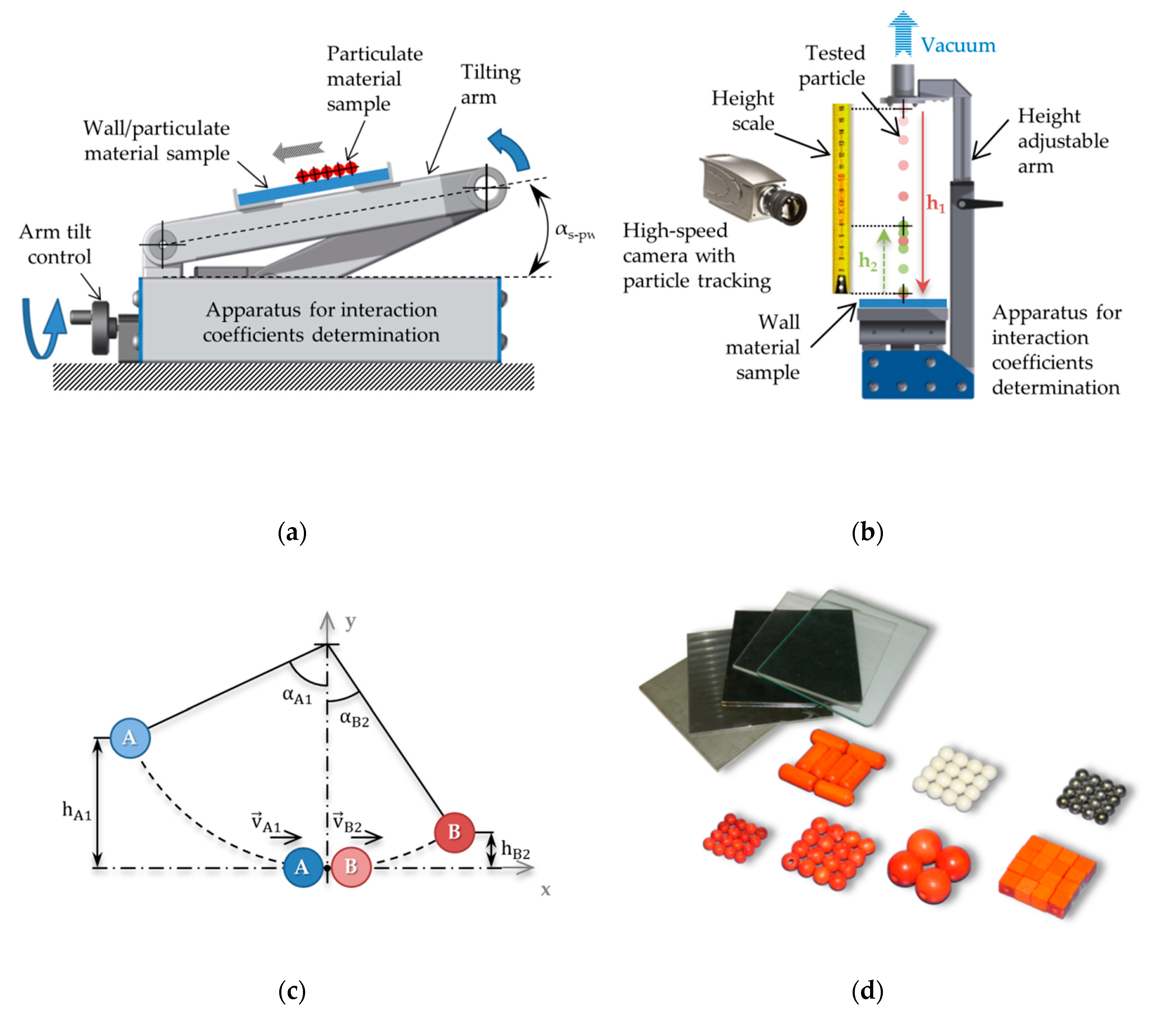
The interaction coefficients define how particles of particulate matter interact with each other or with other materials in contact. The three basic DEM interaction coefficients used in the Hertz-Mindlin contact model include the coefficient of static friction μs, the coefficient of rolling friction μr and the coefficient of restitution e. While some values of these interaction coefficients (e.g., static friction between a particle and a contact material) can be measured quite easily using test apparatus, the experimental determination of the coefficients defining interactions between the particles themselves (and their subsequent use in DEM) is often challenging. In order to measure all three interaction parameters, a test apparatus designed with regard to accuracy and simplicity of measurements was constructed. To measure the coefficient of restitution, the device features a height-adjustable arm with a head. A vacuum source can be connected to this head, allowing one to suck a test particle onto a fine screen of the head. The tilting arm controlled by a screw facilitates a fine pitch for smooth operation serves to measure the friction parameters.
The static friction measurement scheme is shown in Figure 3a. The coefficient of static friction between the particle and the contact material μs–pw is determined from the measured angle αs–pw using the following equation:
μ s p w   =   tan ( α s p w )
Grains of a shape approaching a sphere (i.e., grains start to roll rather than slip on the wall material) are more challenging. This phenomenon has to be eliminated by clumping several particles into one compact unit (clump). In the particle surface thusly formed (see Figure 3d), the free rotation of the grains is prevented, and only static resistance, not rolling resistance, is measured. The same methodology was used to measure the initial static friction values between particles μs–pp, but the contact material was replaced with the surface of another particle clump.
The coefficient of rolling friction has been widely discussed, as evidenced by a number of publications dealing with this topic [16,43]. When spherical particles are used, rolling friction should be included, but this is not necessary when working with non-spherical particles [36]. Wensrich and Katterfeld (2012) discuss this issue in their publications, among others. The same methodology was used for the spherical shape particles as for the measurement of static friction. The rolling friction coefficient for the particle μr is calculated from the measured angle αr according to the following equation:
μ r   =   tan ( α r )
The coefficient of restitution (denoted by e) is the ratio of the final to the initial relative velocity between two objects after they collide. It usually ranges from 0 to 1, where 1 refers to a perfectly elastic collision. The coefficient of restitution can be considered as the degree to which the mechanical energy of bodies is maintained when reflected from a surface or other body. In cases where the frictional forces can be neglected, and in the perfect progression of the collision and bounce, the ratio between the potential energy before the fall EP1 and the potential energy after the reflection EP2 can generally be calculated as follows:
e p w   =   E P 2 ( bounce   height ) E P 1 ( drop   height )   =   m g h 2 m g h 1   =   h 2 h 1
For experimental measurements of the particle-wall restitution coefficient, an apparatus for measuring the interaction coefficients was used (Figure 3b). A vacuum source was attached to a holder mounted on an extendable arm to hold a test particle on the holder screen. After switching off the vacuum source, the particle dropped from the height h1 vertically onto a contact material, from which it bounced to the height h2. The entire course of the experiment was captured using a high-speed camera. The movement was evaluated using tracking software that allows one to accurately track the particle trajectory. After reading the respective drop and rebound heights, the coefficient of restitution was determined according to Equation (5). A method published by Hlosta et al. (2018) was used to measure the coefficient of restitution of two particles. The coefficient of restitution of two particles is based on the laws of momentum conservation and energy conservation. When two particles collide, the total impulse introduced to the system (the two particles) is equal to zero. In the case of the collision of two particles that travel in one plane at different velocities before and after collision, it is assumed that the contact force between the particles is also in the same plane and the state of momentum is maintained. In this case, the coefficient of restitution is defined as the ratio of the relative velocities of the particles before and after they collide. If modelling of the flow of bulk material is required, damping behavior often becomes a factor of secondary importance. This is because many bulk materials demonstrate relatively strong damping properties. In most cases (e.g., in friction dominates processes), a value between 0.2 and 0.4 is appropriate and drop tests can be neglected in order to reduce the number of parameters to be calibrated [36].
Particle A is hanged on a hinge and released from height hA1. At the lowest point, particle A collides with particle B. It transmits its kinetic energy to particle B, which is reflected to the height hB2. The coefficient restitution of two particles can be determined based on the Equation (5). Another way to determine the coefficient of restitution is using the ratio of the angle of reflection αB2 to the angle of drop αA1. The principle of this measurement is shown in Figure 3c. Here again, the coefficient of restitution is a measure of how much energy is lost in a collision. The values range is 0 < e < 1. In an ideal plastic collision (epp = 0), the particles remain together after they collide. In a perfect elastic collision (epp = 1), no energy is lost so that the kinetic energy of the system is maintained and the velocity of the particles after the collision is equal to the velocity preceding the collision. In this study, a two-particle collision experiment using a double pendulum is employed to measure the coefficient of restitution of two particles [44]. All measurements of interaction parameters were repeated ten times for each particulate material. From these ten values, the average value was determined including the standard deviation.

2.2.2. Bulk Density Measurement and Calibration

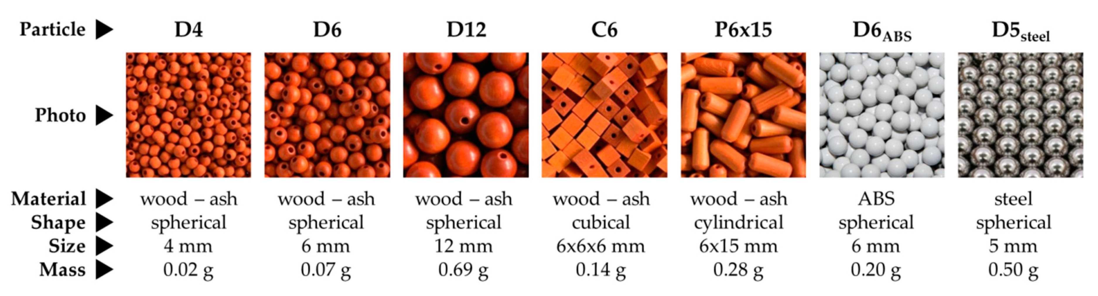
Particles packed in a bed are probably the simplest state of particulate matter, which is present both in nature and in a number of industries. The understanding of the particle deposition is also important in industrial applications due to the particle compaction (which is utilized in powder metallurgy), and the characterization of porosity, since air permeability and thermal conductivity of particulate materials can be quantitatively linked to the pore content and inter-particle contact properties. The bulk density verification parameter was the bed height of a particulate material of a known number of particles in a cylinder during the experiment and the DEM simulation. Differences in the resulting height can be resolved by shape accuracy and particle size. The weight of each individual DEM particle was always identical to the weight of actual particles according to Table 3. The second use of the packing test is the initial estimation and determination of the friction parameters μs and a μr, as the values of static and rolling friction affect the height of a bed [
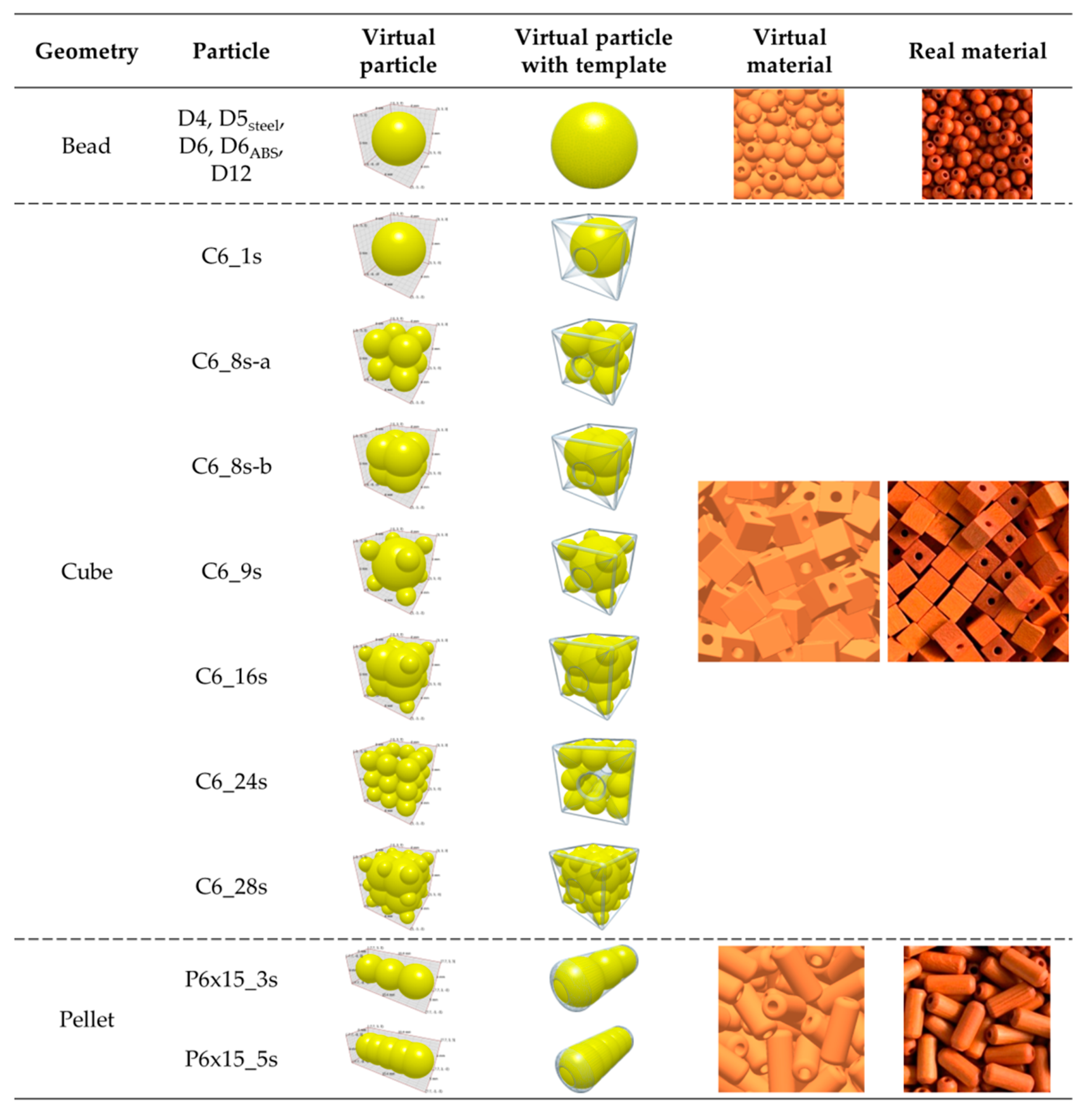
45]. A 1000 mL cylinder, stand, hopper, length gauge, tripod camera and slide shutter were used for the packing test. Each of the seven particulate materials was gradually placed in the hopper above the measuring cylinder and closed by the slide. The slide was then removed, and the material was freely poured into the cylinder. The camera took a photograph which was later used for reading the height of the material bed using the length gauge that was part of the apparatus and was placed in a vertical plane intersecting the axis of the cylinder. This procedure was repeated ten times for each material. From these ten values, the average was determined including the standard deviation. Based on DEM, the computational cost re-calculated to seconds per particle was also recorded as a possible criterion for the subsequent selection of shape accuracy for C6 and P6 × 15 particles. Material constants shown in Table 2 and specific densities of particles in Table 3 were used as input parameters. The scheme and principle used for the packing test are shown in Figure 4.

2.2.3. Shear Modulus Value Optimization

Using Young’s modulus and a shear modulus, respectively, which are lower than their actual values, is common practice in DEM. The main reason is to reduce the computational time. Chen et al. (2017) presented a study on the relationship between Young’s modulus in the range 0.01–0.0001 of the real value of Young’s modulus E0 and the results of DEM simulations in which mixing of particles inside a rotary drum was investigated. The results showed that Young’s modulus has a significant influence on the behavior of individual particles during collisions, but only a small effect when mixing individual layers. Convective mixing due to random particle collisions is negligible compared to diffusion and friction mechanisms. The study also showed that a value of Young’s modulus reduced by up to 0.0007 times of the real value does not affect the results of the mixing simulation, and the DEM models with these values corresponded to the experiments performed. Additionally, the effect of the drum rotation speed or filling level on the relationship between the Young’s modulus value and the simulated mixing results was not observed in Chen’s study [46]. In the case of DEM, isotropic materials, material properties, Young’s modulus E, the shear modulus G and Poisson’s ratio υ are related as follows:
G   =   E 2 ( 1 + υ )
One of the key numbers in DEM simulation is the Rayleigh time step. This is the time taken for a shear wave to propagate through a solid particle. It is therefore a theoretical maximum time step for a DEM simulation of a quasi-static particulate collection in which the coordination number (total number of contacts per particle) for each particle remains above 1. It is given by:
Δ t m a x   =   π R 0.163 υ + 0.8766 ρ G
where R is the particle’s radius, ρ its density, G the shear modulus and ν the Poisson’s ratio. This formula assumes that the relative velocity between contacting particles is very small. Other than for quasi-static systems, in practice some fraction of this maximum value is used, and for high coordination numbers (4 and above) a typical time step of 20% Δtmax has been shown to be appropriate. For lower coordination numbers, 40% Δtmax is more suitable [47]. Choosing a suitable time step represents a compromise between the computational complexity/time, calculation error and simulation stability. Generally, the time step ranges between 20% and 80% of the critical time step according to Rayleigh. With regard to the duration of the calculation and its accuracy, a value of about 30% Δ
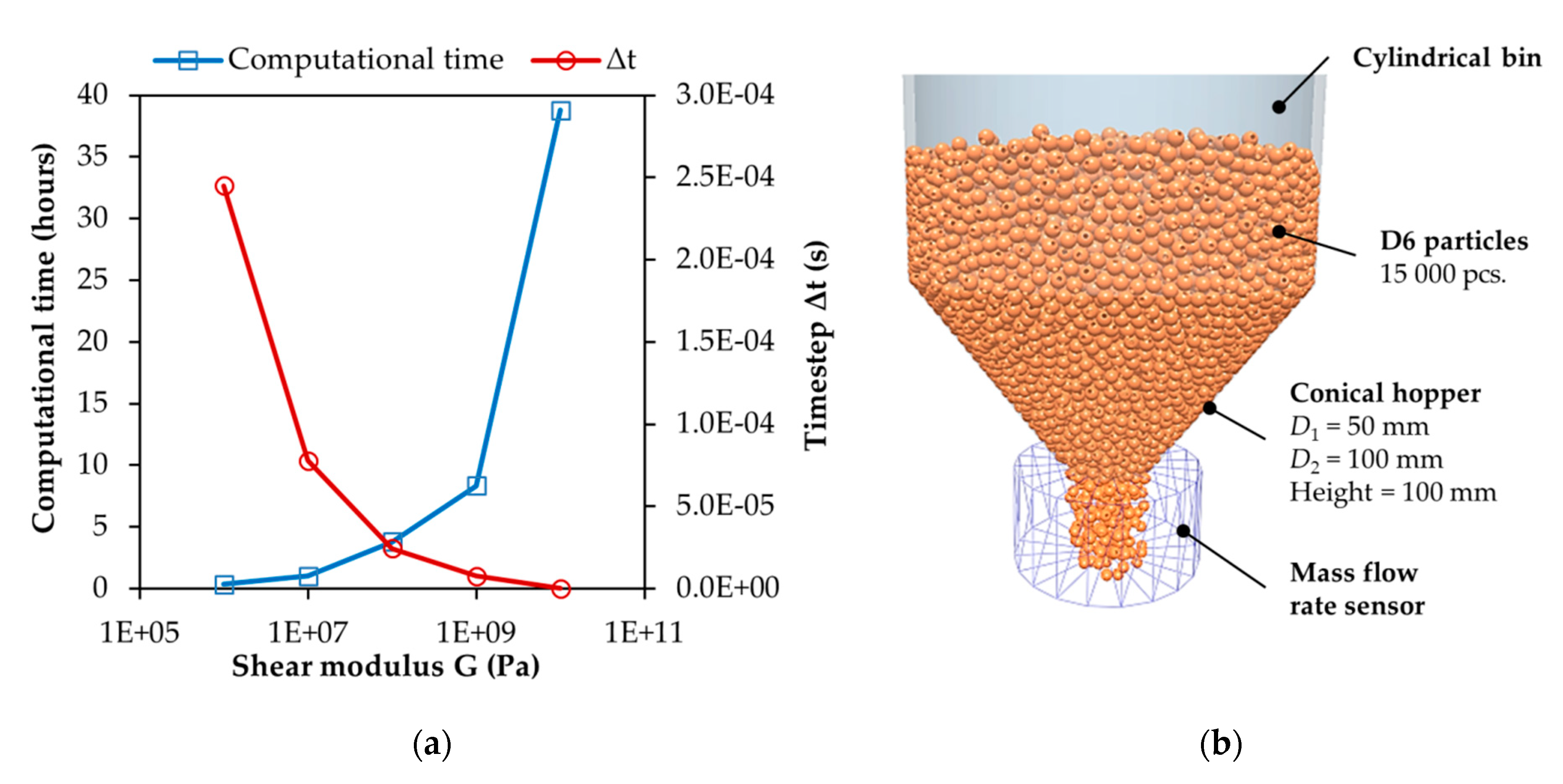
tmax was chosen for all simulations. In the proposed experiment, the influence of the shear modulus value on the process of discharging a hopper was investigated. A virtual cylindrical hopper with a conical discharge hopper of a 50 mm diameter was modelled. The conical hopper of a height of 100 mm was connected to the cylindrical part of a diameter of 100 mm. The experiment was performed for 15,000 pieces of D6 particles generated into the hopper. Subsequently, the flow rate of particles from the discharge hopper and the simulation calculation time were monitored for 5 s.

2.2.4. Static and Dynamic Angle of Repose Test

The process of forming a pile of particles is important in all industries where particulate materials are used. The angle of repose represents one of the basic properties of particulate matter, which affects transport and storage. In contrast to liquids or solids, granular materials create an angle of repose that depends on many of the material’s properties. Parameters such as internal friction between particles, particle size and shape, size distribution, surface, moisture and electrostatic or cohesive forces may influence the value of the natural angle of repose. The angle of repose (static: S-AoR, and dynamic: D-AoR) is also one of the most important parameters for characterizing the flowability of particulate materials. The dynamic angle of repose represents the angle of slope at which a given flowing cohesionless material comes to stable dynamic state. Calibrations based on the angle of repose are generally performed by comparing experiments and simulations on a 1:1 scale. The interaction coefficients can be gradually optimized by systematically changing the input parameters or by simulations managed by the optimization algorithm [48,49]. At the end of the calibration, a set of DEM parameters is determined that provides the closest simulation results to those of the experiment. In particular, rolling and static friction are parameters which affect the macroscopic behavior of cohesionless bulk materials.
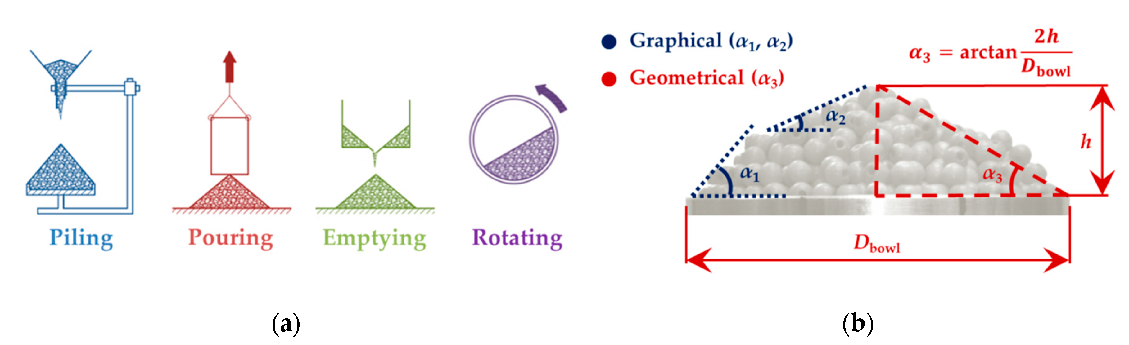
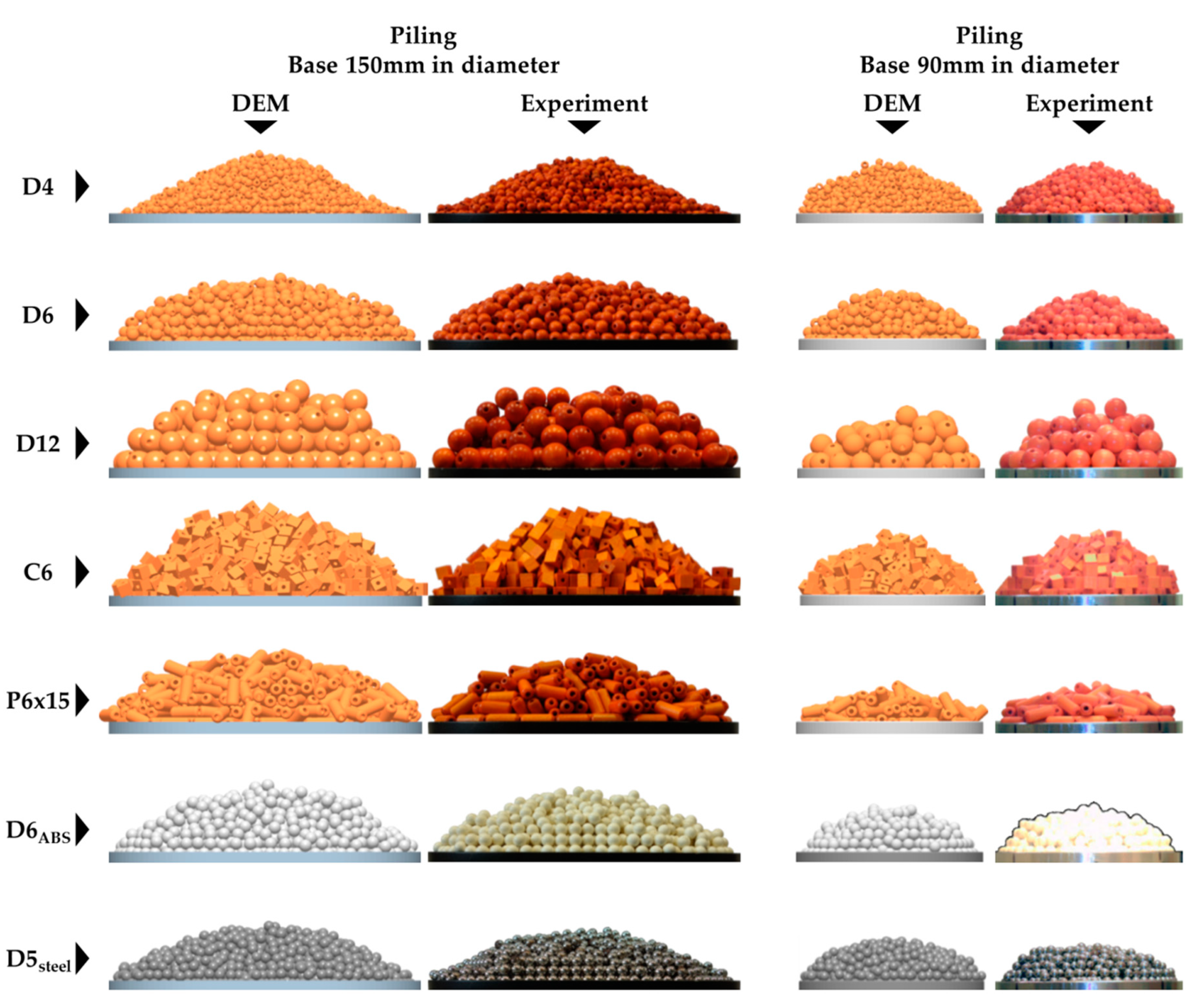
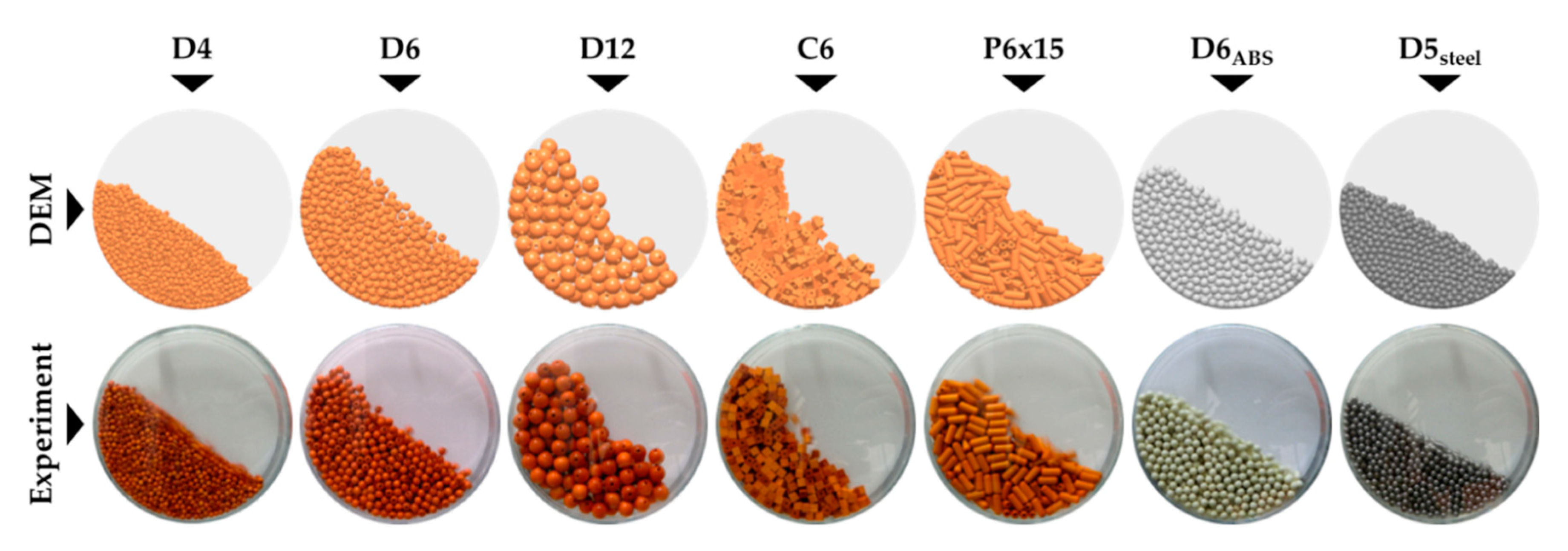
AoR of particulate material is influenced by many factors, such as the static and rolling frictions of particles, particle sizes and shapes, the quantity of material used during measurement and the measurement method (see Figure 5a). It is necessary to choose a particular measurement method based on the application, since each method provides slightly different AoR values. Particular materials were chosen for the experiments with regard to their grain shape so it would be possible to evaluate the advantages and disadvantages of the individual methods. The “piling” and “rotating” methods (see Figure 5a) proved to be the most universal and most credible for the determination of the AoRs of particular materials. If simple conditions are observed, these methods are able to provide high quality AoR values for a wide range of bulk materials. Angle of repose has been widely discussed in the literature for many decades and has been researched by many scientists, even outside of the process engineering field. This issue is first to be divided into two parts: (1) a study of how a pile of particulate material is formed; and (2) how the angle of repose is determined. Piling, pouring, emptying and slowly rotating in a drum leads to the determination of the static angle of repose. The dynamic angle of repose may be obtained in a rotary drum at higher rotational speeds [50]. Each of these methods in a way influences the resulting angle of repose.
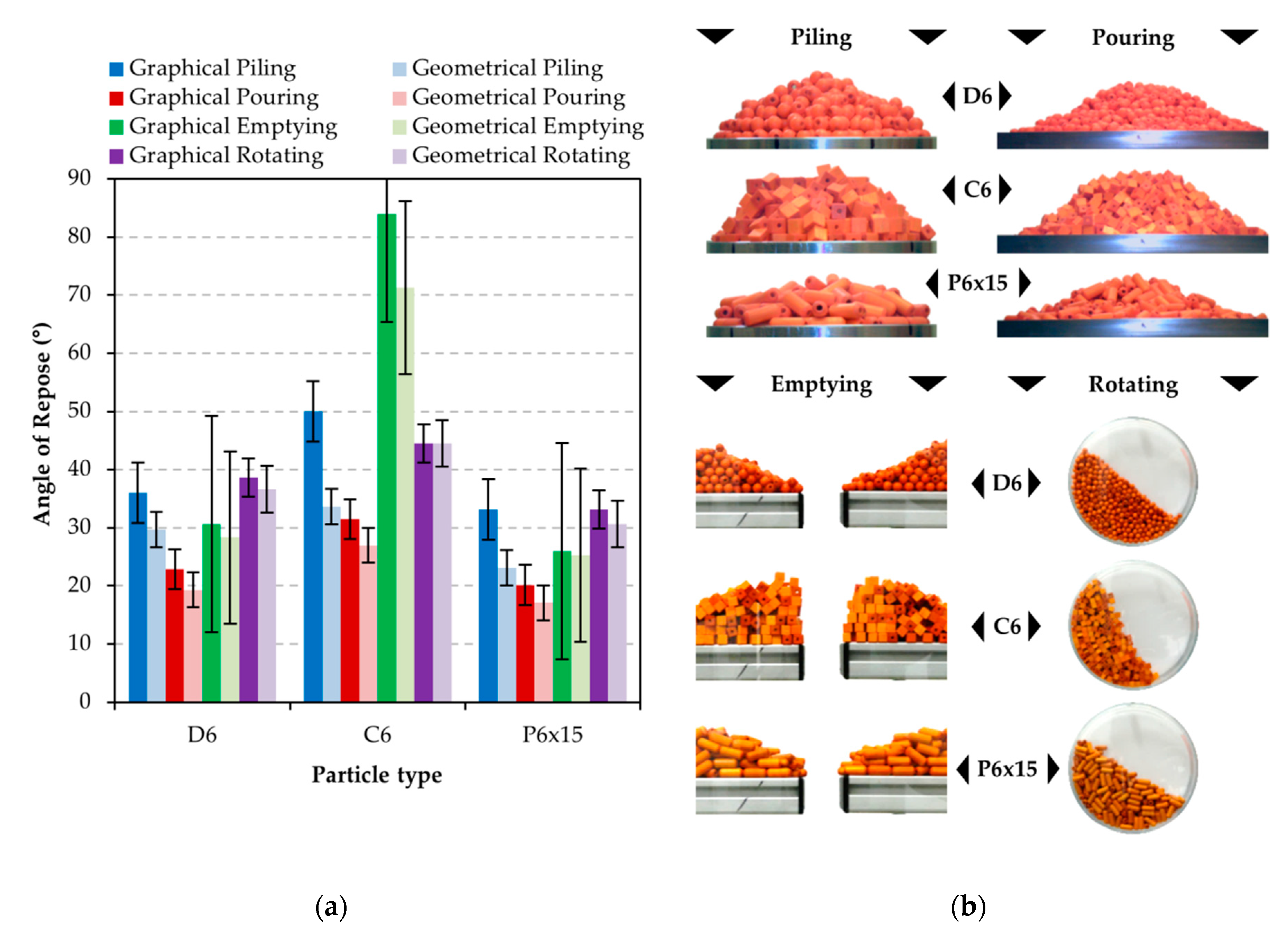
Calibration using the static angle of repose is primarily used to optimize interparticle interaction parameters. For the calibration via the dynamic angle of repose, a rotating drum was used with the static friction between particles and a PMMA cylinder. A rotating drum was also used for an experimental study of homogenization. The drum diameter of 140 mm corresponds to a number of about 25 particles across the surface profile. An adequate number of particles is important for determining the dynamic angle of repose. A low number of particles may lead to distorted results. Similarly, if there are too many particles in the drum, the DEM calculation times increase significantly. As some materials travel in different ways in the drum, their trajectories were in all cases compared with the recordings of the experiment. This comparison allowed for the evaluation of whether a particular material could be retained with existing properties or if any of the parameters needed to be adjusted. Each of methods was evaluated in two ways, both graphically and geometrically (see Figure 6b).

2.2.5. Hopper Discharge Test

The calibration of the virtual material based on the discharge time of the hopper is important not only in terms of setting adequate flow properties, but also the rates of dispersion and diffusion of particles in the volume, which are crucial for all processes involving mixing. For all calibration experiments, it is important to find a suitable compromise between the number of particles used in the calibration test and the calculation time of single experiment. The more particles in one experiment that are calibrated, the more accurate the results which can be achieved. However, the experiments must be well-performed (simple movements of the apparatus, particles must not cause changes in the position of the apparatus, etc.) and reproducible over time. The hopper model was used to calibrate free-flowing materials. After filling the hopper with a particulate material and opening the discharge orifice, the material starts to flow onto a slide and slides/bounces to the bottom part of the model, where it forms a slope of a natural angle of repose. In addition to subjective observation and comparison of the course of the experiment with the simulation, this method makes it possible to calibrate the material using several different quantifiable aspects. For example, the particle speed at various points, particle tracking, the angle of repose defined after the experiment, the flow through the discharge orifice, the discharge time of the hopper and the mass loss characteristics of the hopper over time. Another option would be to use PIV analysis and compare the shape of vector fields with quantifiable velocity results. The inclination of the walls of the hopper and the slide is variable and the size of the discharge orifice and can be adjusted according to the material being calibrated.
In this study, calibration was based on the discharge time of the hopper, which contained a given number of particles. Furthermore, a visual assessment of the material flow from the hopper and through the slide was performed. First, an experiment was performed for each particle type. The hopper inclination was 60° in all cases while the discharge orifice width was set for each material so that the particles could flow freely. The whole experiment was recorded at a frame rate of 240 fps. Therefore, the exported record could to be slowed down to 12% of the real time of the experiment. This made it possible to determine the time period from opening the discharge orifice to the point when the last particle left the hopper with an accuracy of 0.004 s. DEM simulations were saved in steps of 0.01 s. Interaction parameters were then optimized and validated for the static and dynamic angles of repose.

3. Results

3.1. Particles’ Shapes and the Packing Test

A series of simulations was performed during the course of the packing test to initially estimate the friction parameters of the contact model. For spherical particles D6, cubic particles C6_24s and cylindrical particles P6 × 15_5s, 56 simulations of the packing test described in Section 2.2.2 were performed for each particle. The simulations involved combinations of static and rolling friction in the range of μ s pp = 0.05 , 1.5 and μ r pp   =   0.005 , 1.5 . Table 4, Table 5 and Table 6 show the results of percentage-wise deviations from real experiments, in which the particle bed height for a given number of particles was 184 ± 1.3 mm for D6 particles, 202 ± 1.8 mm for C6 particles and 190 ± 1.6 mm for P6 × 15 particles (as shown in Table 3.). Thus, friction parameters can be gradually optimized by systematically changing input parameters or by simulations managed by the optimization algorithm. By gradual refinement of the friction scale values at the points of best match, more accurate estimates of the input parameters can be achieved. These frictional parameter estimates can then be combined with experimental static friction measurement to optimize the rolling friction coefficient, which is experimentally more difficult to determine. This can also solve the situation where multiple combinations provide an equal match to the experiment; e.g., μs–pp = 0.1 and μr–pp = 0.5; and μs–pp = 0.2 and μr–pp = 0.5 for D6 particles (see Table 4).
The results of the calibration experiment involving volume filling are shown in Table 7. Based on Table 4, Table 5 and Table 6, initial friction parameters were used as follows: μs–pp = 0.5 and μr–pp = 0.1 for cubical and cylindrical particles C6 and P6 × 15; and μs–pp = 0.2 and μr–pp = 0.01 for spherical particles D4, D6, D12, D6ABS and D5steel. This table demonstrates that only virtual particles D6ABS, D5steel and C6 wooden cubes achieved an acceptable deviation of up to 5%, but C6 particles required much longer computational time. Therefore, it is necessary to optimize the size of all other virtual particles so that it better corresponds to the real experiment. The C6_24s particle was chosen as the virtual particle of the wooden cube for this study due to its geometric representation of the actual particle and due to the acceptable computation time per particle. This ratio was used like one of the criteria during the particle clump selection. The virtual particles D4, D6, D12 and C6_24s were subsequently enlarged by 0.2 mm in their characteristic dimension. Particles D6ABS and D5steel were kept in their original state. Virtual particle P6 × 15_5s was chosen for simulation of 15 × 6 mm pellets. This was also unchanged due to the very good result of the calibration experiment with a 0.5% deviation. The results of the optimized particles already showed very good agreement with the experimental data. The bulk density calibration for complex polydisperse particulate materials could be solved in a similar way which would allow for the determination of the best correlations between particle size distribution, density, friction parameters and particle bed height. The mass of the particle bed has to conserve the real mass of material in the case of particle size distribution (PSD) and/or particle size simplification by particle density setting.

3.2. Interaction Parameters’ Determination

Table 8 shows the coefficient of static friction of particles for different contact materials. The methodology described in Section 2.2.1 was used. In all cases, the standard deviation was based on ten repetitions of individual experiments. The measurements were influenced mainly by the quality of the surfaces of contact materials, the orientation of the particle surfaces and the speed of arm tilting. The measured values reflect the actual physical properties of the particles and could be used for the contact model, but it may be necessary to adjust them in conjunction with calibration experiments. Shear friction depends primarily on the quality of the contact surfaces, which also represents a problem in practice. The movement of particulate matter along the contact surfaces causes their degradation or even polishing. For this reason, the coefficient of static friction between particles and contact surfaces may change over time. In the case of wooden beads and their static friction, it is important whether a bead hole is placed on the wall material surface or not. The results can also be affected by the processing and finish quality of individual beads or the direction of tooling. In plastic particles placed on plexiglass, the friction can also be affected by electrostatic charge, etc. Experimentally measured values of static friction show the predicted range from 0.2 to 0.5. The same methodology was used to measure the mutual static friction between the particles, only the wall material sample was replaced with the surface of another particle. The static friction coefficients of individual particle combinations are shown in Table 9.
The results of rolling friction measurements shown in Table 10 are based on the same measurement methodology as that described in the previous Section 2.2.1, except that the entire particle was used for the measurement instead of the particle surface. Except for C6 particles, all other particles had a spherical shape. They had a much smaller rolling friction coefficient than the static coefficient. Therefore, the tilt of the arm on the apparatus can be used to determine the moment when a particle starts to roll and determine the rolling friction coefficient using the Equation (4). For particle C6, the default value μr–pw = 0.5 was chosen based on the packing test due to difficult/impossible experimental determination. The particles were tested on a steel wall material, and one global particle-wall rolling friction coefficient was used for each particle for the next calibration experiments. In determining the coefficient of rolling friction, it is essential that the axis of the cylindrical particle remains perpendicular to the direction of motion throughout the experiment.
The values of the coefficient of restitution (CoR) between individual particles and contact materials are shown in Table 11. The drop test methodology chosen and often discussed in the literature is very well applicable to spherical particles in which the trajectory of drop and reflection takes place in one plane. However, a problem arises with non-spherical particles, in which the reflection trajectory depends on the position of the particle upon collision with the contact material. If the material is reflected off the recorded plane, the velocity vector decomposes into individual components, thereby distorting the resulting value of the coefficient of restitution. As a result, the Equation (5) becomes inaccurate, and it is necessary to evaluate the reflection based on the speed in all directions. Furthermore, in this experiment, it is necessary to ensure sufficient stiffness of the contact material sample to prevent reflection damping caused by its deformation. The pendulum method with one hinge with the test particle and a vertically placed wall sample was used for C6 particle coefficient of restitution determination. This test used a method shown in Figure 3c, but particle B was replaced by fixed wall sample. CoR was determined using the Equation (5) in the same way as in the case of a two-particle collision.
The double pendulum method described in Section 2.2.1 (see Figure 3c) was used to measure the coefficient of restitution of two particles. Table 12 shows the coefficients of restitution for particle interactions. The values of the coefficient of restitution were determined according to the heights and the angles of drop and rebound. These measurements were performed only for pairs of the same particles due to their identical weights. Other values of the coefficient of restitution for mutual combinations of different particles were determined according to the following equation [51]:
e p p   =   E A · e A + E B · e B E A + E B

3.3. Shear Modulus Value Optimization

Following the conclusions made by Chen et al. (2017) in their study on the influence of Young’s modulus on the process of mixing in a rotary cylinder, and the knowledge gained during the experiments with hopper discharging, it can be stated that the reductions of Young’s modulus and the shear modulus, respectively, do not affect the courses of these processes in which the particles interact at low speeds. Figure 6 and Table 13 demonstrate that even a shear modulus change in the range of 104 Pa did not affect the flow properties of the material during the process of discharging. Different particles shapes achieved very similar results with slight differences of shear modulus of between 1 × 10⁶ and 1 × 10¹⁰ Pa. Bin discharge simulations exhibited very good reproducibility of results. The number of emptied particle differences was 0.5% maximally during simulation repetitions. Conversely, the calculation time increases exponentially as the value of the shear module increases. With suitable optimization, qualitatively comparable results can be achieved in much less time. In complex models with large amounts of particles, this could lead to potential time savings of several days. The optimal value of 0.001 times of the actual values was chosen (i.e., they are converted from gigapascals to megapascals).

3.4. Angle of Repose Calibration Tests

At first, a comparative measurement of four methods of determination of the angle of repose for particulate materials was performed. Each of these four methods (see Figure 5a) was evaluated in two ways, both graphically and geometrically (see Figure 5b). For each of the three selected materials (spherical D6, cubical C6 and cylindrical P6 × 15) ten measurements were made for each measurement method. A comparison of the resulting AoR values is shown in the graph in Figure 7a. The results show the differences between the methods, not only in the form of a pile but also in the method of measurement evaluation. Figure 7b shows experimental results of different pile formation methods.
All materials were first tested with a “piling” method. Here the measurement is influenced mainly by the ratio of the particle size to the diameter of the bowl onto which the material is piled. Furthermore, the measurement is influenced by the height at which the material is dosed, as at too great a height the pile is disintegrated by the falling grains. For the “pouring” method, the shape of pile is informed by the speed at which the cylinder is lifted, and the friction between the cylinder wall and the bulk material. If the cylinder is lifted too fast, the material does not spill out of the cylinder immediately due to friction and inertia, but rather with a delay when the cylinder is at a certain height above the bowl, which results in a larger “spill” of the material on the surface. For the “emptying” method, care must be taken to ensure that the size of the drain hole is sufficient to avoid particle bridging, while in the “rotation” method a sufficiently low speed allowing static AoR must be observed. Ten piles were created for each material, and every pile was photographed from four views. Autodesk AutoCAD was used for manual repose angle determination. Two angles of repose were determined per picture (both sides of pile). All of values obtained were averaged, including relative standard deviation (RSD) determination.
Figure 7a,b show the results of all experiments with wood particles of different shapes. Some of the methods prove to be unsuitable for certain shapes and sizes. For example, for the “piling” method, the bowl is too small for the P6 × 15 particles and the particles are unable to form a proper cone to measure the angle of inclination. The evaluation of this method by an operator is then a highly subjective. Moreover, the “emptying” method proved to inappropriate for C6 particles, since we observed bridging above drain hole or the strong core flow, when only the particles above the drain hole were dropped, creating a slope angle of almost 90°.
Figure 7a shows the tendency of the individual methods of pile formation towards higher or lower AoR values. The “pouring” method had the lowest AoR values, which were close to the dynamic AoR. Thus, the method can be used, for example, for the capacity calculations of belt conveyors, etc. On the other hand, the “emptying” method showed the highest AoR values and a large deviation between the measurements. The rotating drum method showed very stable and consistent results. We also observed differences between the two methods of evaluation of experiments, as the geometric evaluation showed lower AoR values. Based on introductory AoR experiments, pilling and rotating methods have been selected for the DEM calibration process. These two methods exhibit the most stable results and high usability for different particle shapes. In some cases, the calibration using piling method with a small bowl and a small number of particles is more difficult than the calibration of a big pile on the free surface. Performing both ways together with a rotating drum experiment is the optimal situation. Graphical evaluation of the piling method gives closer results to the rotation drum method, so it was used for AoR evaluation in all cases. However, it is advisable to observe the overall shape of the pile; e.g., the roundness of the pile tip.
The results of calibration experiments for the determination of the static angle of repose are shown in Figure 8 and Table 14 and Table 15. Materials D4, D6, D12, P6 × 15 and D6ABS kept their experimentally measured input parameters. For material C6, the value of the rolling friction coefficient was adjusted from 0.50 to 0.15; for material P6 × 15 the value of rolling friction was changed from 0.06 to 0.03, while the value of static friction between particles was changed from 0.40 to 0.25. Similarly, for steel spheres D5steel, the value of rolling friction was adjusted from 0.02 to 0.03, and the value of static friction between particles from 0.17 to 0.30.
Figure 9 shows a comparison of the behaviors of all particulate materials at a drum speed of 6 rpm. For material D6, the static friction coefficient between the particles and the PMMA cylinder wall was adjusted from 0.54 to 0.35. The behaviors of the other materials showed satisfactory results with the original experimentally measured and calibrated parameters. Ten measurement repetitions were made for each experiment. Based on good reproducibility of DEM simulations, the first calibration simulation was performed for the AoR determination and the second simulation for agreement of the results of every particle series. The final AoR values of calibrated materials are shown in Table 14 and Table 15.

3.5. Discharge Test

The discharge test was performed according to the methodology described in Section 2.2.5. The results of the calibration tests based on the discharge time of the hopper are shown in Figure 10 and summarized in Table 16. Figure 10 shows the different phases of the discharge of the hopper model. Comparisons of the experiment and the DEM model for the individual particles were captured at the same time; i.e., at the same time from the release. The discharge test represents a rather versatile calibration tool. It allows one to calibrate the flow properties given by the friction parameters, and the slip and bouncing of the particle flow from the slide, and grants the option to use various contact materials. Another way to evaluate the discharge test is to monitor the movement of particle layers of different colors or to evaluate velocity fields using PIV analysis. In this study, the discharge times of the specified numbers of particles were used for comparisons. Furthermore, the recordings of experiments and DEM simulations were visually compared. Some of the input parameters of the DEM contact model were further refined by this calibration test and back-tested.

4. Discussion

The simple shapes of some products can be easily achieved by the “clumping” method (e.g., agricultural commodities such as rice, cereals and pellets). The higher the number of spherical surfaces, the higher the accuracy that can be obtained when approaching real morphology. However, the computational power required to calculate the contact forces between particles with a large number of surfaces increases significantly.
The first calibration experiment involved filling the volume of a cylinder (the so-called “packing test”) to determine the shape accuracy and bulk density of each virtual material. The series of simulations was compared with real experiments, and the sizes, shapes and densities of virtual particles were optimized. The computational costs of a particle made up of more than one spherical surface were recorded. It represented one of the parameters that played a role in the selection of the creation method of the resulting cubic particle. Interestingly, cubic particles C6 formed from 24 spherical surfaces showed less computational complexity than particles C6 with 16 spherical surfaces. This was due to the larger particle diameters and the longer computation time step. However, this parameter had only minimal influence in the case of pellet particle P6 × 15.
Three test apparatuses were designed and assembled for the following series of calibration experiments. Namely, an apparatus for measuring the interaction coefficients (i.e., the static friction coefficient, rolling friction coefficient and coefficient of restitution); a rotary drum apparatus for measuring the dynamic angle of repose and flow properties; and a hopper model for dynamic flow monitoring, which allows for the calibration of virtual materials according to the flow method (mass vs. core), angle of repose, discharge time, etc. Using these three apparatuses, the input parameter values were experimentally determined for a contact model that defines the behavior of particulate materials in DEM simulations.
The influence of the shear modulus value was investigated during the calibration of the virtual material. This part of the paper showed that the use of a shear modulus value three orders of magnitude lower (from GPa to MPa) than the tabulated values for a given material does not affect the material behavior in the simulations. Shear modulus values do not affect the flows of differently shaped particles. Indeed, this simplification has a significant impact on the simulation computation time, which can be reduced by up to 35 times. Furthermore, the interaction parameters were calibrated and optimized based on the static and dynamic angle of repose or discharge time of the hopper model. The AoR of a particulate material is influenced by many factors, such as the static and rolling friction of particles, particle sizes and shapes, quantity of material used during measurement and the measurement method. This study performed comparative measurements of differently shaped materials using different methods of pile formation. The results show that it is necessary to choose a particular measurement method based on the application, since each method provides slightly different AoR values. Particular materials were chosen for the experiments with regard to their particle shape, so that it would be possible to evaluate the advantages and disadvantages of the individual methods. The “piling” and “rotating” methods proved to be the most universal and most credible for determination of AoR of particular materials. If simple conditions are observed, these methods are able to provide high quality AoR values for a wide range of bulk materials.
These practical tests helped to refine some of the interaction coefficients, which are difficult to determine experimentally. Thus, an optimal relation between the set of all interaction coefficients was found, since the mutual combination of these values defines the behavior of a particulate material. However, even if the individual coefficients are determined relatively accurately, their combination in the contact model used may not reflect the actual behavior of the particular material due to some further simplifications. All calibrated DEM parameters of investigated particulates are mentioned in Table A1, Table A2, Table A3, Table A4, Table A5, Table A6 and Table A7 in Appendix A.

5. Conclusions

  • The packing test can be used for initial estimation and to optimize and find a suitable combination of the input parameters for the DEM contact model. Furthermore, the packing test is a suitable tool for optimizing the shape representation of particles and bulk density.
  • For the Hertz-Mindlin contact model, the coefficient of static friction and the coefficient of restitution can be relatively easily determined experimentally. In addition to these values, it is necessary to find a suitable rolling friction coefficient to ensure both the static and dynamic behavior of the material.
  • By optimizing the shear modulus, the computational time of the simulation can be significantly reduced. Even a shear modulus reduction by 104 Pa does not affect the flow properties of the material.
  • Calibration using a static AoR is generally the most commonly used calibration experiment. However, the results are influenced by many factors, such as the number of particles, the forming method of the pile and the method of evaluating the final value of the AoR. During selection of a suitable calibration methodology, it is necessary to base it on the simulated process and material properties.
  • The most reproducible results of the angle of repose were achieved by the “pilling” method and in the rotating drum when evaluated by the geometric method. However, it is always advisable to make an overall visual comparison of the slope shape between the calibration simulation and the experimental curves. The base to particle size ratio should be greater than 25, and the calibration experiment should contain approximately 4000 particles to ensure representative and reproducible results.
  • Dynamic behavior must be verified in the same way as static. Discharge test is a suitable tool for assessing flow properties. One set of input parameters must then best characterize the static and dynamic behavior of the material.

Author Contributions

Conceptualization, J.H. and D.Ž.; formal analysis, J.H.; funding acquisition, J.N. and J.Z.; investigation, J.H., L.J. and J.R.; methodology, J.H., L.J. and J.R.; project administration, J.N.; supervision, J.N. and J.Z.; validation, J.H., L.J. and J.R.; visualization, J.H.; writing—original draft, J.H.; writing—review and editing, L.J., J.R. and D.Ž. All authors have read and agreed to the published version of the manuscript.

Funding

This study was conducted within the framework of the project CZ.1.05/2.1.00/19.0389: Research Infrastructure Development of the CENET; and within the framework of the project SP2020/19: Research in the field of effects of abrasive bulk solids on process equipment. The paper has been done in connection with project Innovative and additive manufacturing technology—new technological solutions for 3D printing of metals and composite materials, regulation number CZ.02.1.01/0.0/0.0/17_049/0008407, financed by the Structural Founds of the European Union.

Conflicts of Interest

The authors declare no conflict of interest.

Nomenclature

Symbols used
Ddiameter(m)
EYoung’s modulus(Pa)
ecoefficient of restitution(−)
Fforce(N)
Gshear modulus(Pa)
hheight(m)
kcontact stiffness(N∙m−1)
Llength(m)
mmass(kg)
Rparticle radius(m)
ttime(s)
vvelocity(m∙s−1)
Greek letters
αtilt, slope angle(°)
δdisplacement(m)
μfriction coefficient(−)
υPoisson’s ratio(−)
ρdensity(kg∙m−3)
ψdamping coefficient(−)
Subscripts
0real
*equivalent
DEMdiscrete element method
drumdrum
expexperimental
iparticle i
jparticle j
maxmaximal
nnormal
pparticle
rrolling
sstatic
ttangential
wwall

Abbreviations

ABSacrylonitrile butadiene styrene
AoRangle of repose
CoRcoefficient of restitution
DEMdiscrete element method
PIVparticle image velocimetry
PMMApoly(methyl methacrylate)
PSDparticle size distribution
RSDrelative standard deviation

Appendix A

Table A1. Mechanical properties used in the DEM model.
SteelAluminumGlassPMMAABSWood (Ash)
Densityρ(kg∙m−3)78502700260012501050720
Young‘s modulusE(MPa)210697032.2511
Poisson’s ratioυ(−)0.30.330.220.40.350.44
Table A2. Calibrated DEM particles’ densities.
D4D6D12C6P6 × 15D6ABSD5steel
Densityρ(kg∙m−3)567569726106176717687639
Table A3. Calibrated coefficients of restitution values (CoR particle-particle).
Coefficient of Restitution epp (−)
D4D6D12C6P6 × 15D6ABSD5steel
D40.61
D60.670.75
D120.670.730.73
C60.660.720.720.70
P6 × 150.700.760.760.740.78
D6ABS0.650.750.750.730.800.87
D5steel0.84 0.840.840.840.850.850.85
Table A4. Calibrated coefficients of restitution values (CoR particle-wall).
Coefficient of Restitution epw (−)
SteelPMMAAluminumGlass
D40.440.490.480.46
D60.420.470.550.46
D120.450.350.500.45
C60.200.290.230.28
P6 × 150.310.370.360.37
D6ABS0.720.620.670.71
D5steel0.260.400.330.68
Table A5. Coefficient values of contact static friction (particle-particle).
Coefficient of Static Friction μs–pp (−)
D4D6D12C6P6 × 15D6ABSD5steel
D40.65
D60.520.44
D120.400.220.45
C60.480.360.410.45
P6 × 150.460.410.390.420.25
D6ABS0.350.380.290.510.440.35
D5steel0.260.260.190.160.290.180.30
Table A6. Coefficient values of contact static friction (particle-wall).
Coefficient of Restitution epw (−)
SteelPMMAAluminumGlass
D40.490.600.150.54
D60.360.350.150.37
D120.350.400.300.35
C60.430.490.200.40
P6 × 150.360.440.200.35
D6ABS0.490.600.220.43
D5steel0.130.150.150.22
Table A7. Coefficient values of contact rolling friction.
Coefficient of Rolling Friction 1
μr–pp (−)
Coefficient of Rolling Friction 2
μr–pw (−)
D40.120.05
D60.080.06
D120.040.05
C60.080.06
P6 × 150.030.06
D6ABS0.030.025
D5steel0.030.02
1 Rolling friction coefficient values for particle combinations were generated by the arithmetic means of the two values of the interacting particles. 2 One global rolling friction coefficient was used for all contact materials.

References

  1. Roessler, T.; Katterfeld, A. Scaling of the angle of repose test and its influence on the calibration of DEM parameters using upscaled particles. Powder Technol. 2018, 330, 58–66. [Google Scholar] [CrossRef]
  2. Al-Hashemi, H.M.B.; Al-Amoudi, O.S.B. A review on the angle of repose of granular materials. Powder Technol. 2018, 330, 397–417. [Google Scholar] [CrossRef]
  3. Qi, L.; Chen, Y.; Sadek, M. Simulations of soil flow properties using the discrete element method (DEM). Comput. Electron. Agric. 2019, 157, 254–260. [Google Scholar] [CrossRef]
  4. Nakashima, H.; Shioji, Y.; Kobayashi, T.; Aoki, S.; Shimizu, H.; Miyasaka, J.; Ohdoi, K. Determining the angle of repose of sand under low-gravity conditions using discrete element method. J. Terramech. 2011, 48, 17–26. [Google Scholar] [CrossRef]
  5. Khanal, M.; Elmouttie, M.; Adhikary, D. Effects of particle shapes to achieve angle of repose and force displacement behaviour on granular assembly. Adv. Powder Technol. 2017, 28, 1972–1976. [Google Scholar] [CrossRef]
  6. Grima, A.P.; Wypych, P.W. Discrete element simulations of granular pile formation: Method for calibrating discrete element models. Eng. Comput. 2011, 28, 314–339. [Google Scholar] [CrossRef]
  7. Coetzee, C.J. Review: Calibration of the discrete element method. Powder Technol. 2017, 310, 104–142. [Google Scholar] [CrossRef]
  8. Zhou, H.; Hu, Z.; Chen, J.; Lv, X.; Xie, N. Calibration of DEM models for irregular particles based on experimental design method and bulk experiments. Powder Technol. 2018, 332, 210–223. [Google Scholar] [CrossRef]
  9. Ye, F.; Wheeler, C.; Chen, B.; Hu, J.; Chen, K.; Chen, W. Calibration and verification of DEM parameters for dynamic particle flow conditions using a backpropagation neural network. Adv. Powder Technol. 2019, 30, 292–301. [Google Scholar] [CrossRef]
  10. Coetzee, C.J. Particle upscaling: Calibration and validation of the discrete element method. Powder Technol. 2019, 344, 487–503. [Google Scholar] [CrossRef]
  11. Coetzee, C.J. Calibration of the discrete element method and the effect of particle shape. Powder Technol. 2016, 297, 50–70. [Google Scholar] [CrossRef]
  12. Saeed, M.K.; Siraj, M.S. Mixing study of non-spherical particles using DEM. Powder Technol. 2019, 344, 617–627. [Google Scholar] [CrossRef]
  13. Rozbroj, J.; Zegzulka, J.; Nečas, J.; Jezerská, L. Discrete element method model optimization of cylindrical pellet size. Processes 2019, 7, 101. [Google Scholar] [CrossRef] [Green Version]
  14. Markauskas, D.; Ramírez-Gómez, Á.; Kačianauskas, R.; Zdancevičius, E. Maize grain shape approaches for DEM modelling. Comput. Electron. Agric. 2015, 118, 247–258. [Google Scholar] [CrossRef]
  15. Simons, T.A.; Weiler, R.; Strege, S.; Bensmann, S.; Schilling, M.; Kwade, A. A ring shear tester as calibration experiment for DEM simulations in agitated mixers–a sensitivity study. Procedia Eng. 2015, 102, 741–748. [Google Scholar] [CrossRef] [Green Version]
  16. Wensrich, C.M.; Katterfeld, A. Rolling friction as a technique for modelling particle shape in DEM. Powder Technol. 2012, 217, 409–417. [Google Scholar] [CrossRef]
  17. Barrios, G.K.; de Carvalho, R.M.; Kwade, A.; Tavares, L.M. Contact parameter estimation for DEM simulation of iron ore pellet handling. Powder Technol. 2013, 248, 84–93. [Google Scholar] [CrossRef]
  18. Wensrich, C.M.; Katterfeld, A.; Sugo, D. Characterisation of the effects of particle shape using a normalised contact eccentricity. Granul. Matter 2014, 16, 327–337. [Google Scholar] [CrossRef]
  19. Cunha, R.N.; Santos, K.G.; Lima, R.N.; Duarte, C.R.; Barrozo, M.A.S. Repose angle of monoparticles and binary mixture: An experimental and simulation study. Powder Technol. 2016, 303, 203–211. [Google Scholar] [CrossRef]
  20. Favier, J.F.; Abbaspour-Fard, M.H.; Kremmer, M. Modeling nonspherical particles using multisphere discrete elements. J. Eng. Mech. 2001, 127, 971–977. [Google Scholar] [CrossRef]
  21. Parafiniuk, P.; Molenda, M.; Horabik, J. Influence of particle shape and sample width on uniaxial compression of assembly of prolate spheroids examined by discrete element method. Phys. A 2014, 416, 279–289. [Google Scholar] [CrossRef]
  22. Markauskas, D.; Kačianauskas, R.; Džiugys, A.; Navakas, R. Investigation of adequacy of multi-sphere approximation of elliptical particles for DEM simulations. Granul. Matter 2010, 12, 107–123. [Google Scholar] [CrossRef]
  23. Soltanbeigi, B.; Podlozhnyuk, A.; Papanicolopulos, S.A.; Kloss, C.h.; Pirker, S.; Ooi, J.Y. DEM study of mechanical characteristics of multi-spherical and superquadric particles at micro and macro scales. Powder Technol. 2018, 329, 288–303. [Google Scholar] [CrossRef] [Green Version]
  24. You, Y.; Li, Y.; Luo, Z.; Li, H.; Zou, Z.; Yang, R. Investigating the effect of particle shape on the charging process in melter gasifiers in COREX. Powder Technol. 2019, 351, 305–313. [Google Scholar] [CrossRef]
  25. Fang, Z.Q.; Hu, G.M.; Du, J.; Fan, Z.; Liu, J. A contact detection algorithm for multi-sphere particles by means of two-level-grid-searching in DEM simulations. Int. J. Numer. Meth. Eng. 2015, 102, 1869–1893. [Google Scholar] [CrossRef]
  26. Cabiscol, R.; Finke, J.H.; Kwade, A. Calibration and interpretation of DEM parameters for simulations of cylindrical tablets with multi-sphere approach. Powder Technol. 2018, 327, 232–245. [Google Scholar] [CrossRef]
  27. Meng, X.; Jia, F.; Qiu, H.; Han, Y.; Zeng, Y.; Xiao, Y.; Chen, P. DEM study of white rice separation in an indented cylinder separator. Powder Technol. 2019, 348, 1–12. [Google Scholar] [CrossRef]
  28. Horabik, J.; Molenda, M. Parameters and contact models for DEM simulations of agricultural granular materials: A review. Biosyst. Eng. 2016, 147, 206–225. [Google Scholar] [CrossRef]
  29. Marigo, M.; Stitt, E.H. Discrete element method (DEM) for industrial applications: Comments on calibration and validation for the modelling of cylindrical pellets. KONA Powder Part. J. 2015, 32, 236–252. [Google Scholar] [CrossRef] [Green Version]
  30. Zhou, Y.C.; Wright, B.D.; Yang, R.Y.; Xu, B.H.; Yu, A.B. Rolling friction in the dynamic simulation of sandpile formation. Phys. A 1999, 269, 536–553. [Google Scholar] [CrossRef]
  31. Wang, Y.; Alonso-Marroquin, F.; Xue, S.; Xie, J. Revisiting rolling and sliding in two-dimensional discrete element models. Particuology 2015, 18, 35–41. [Google Scholar] [CrossRef]
  32. Podlozhnyuk, A.; Pirker, S.; Kloss, C. Efficient implementation of superquadric particles in Discrete Element Method within an open-source framework. Comput. Part. Mech. 2017, 4, 101–118. [Google Scholar] [CrossRef] [Green Version]
  33. Scheffler, O.C.; Coetzee, C.J.; Opara, U.L. A discrete element model (DEM) for predicting apple damage during handling. Biosyst. Eng. 2018, 172, 29–48. [Google Scholar] [CrossRef] [Green Version]
  34. Roessler, T.; Katterfeld, A. DEM parameter calibration of cohesive bulk materials using a simple angle of repose test. Particuology 2019, 45, 105–115. [Google Scholar] [CrossRef]
  35. Nikolakakis, I.; Pilpel, N. Effect of particle shape on the tensile strengths of powders. Powder Technol. 1985, 42, 279–283. [Google Scholar] [CrossRef]
  36. Katterfeld, A. Calibration of DEM Parameters for Cohesionless Bulk Materials under Rapid Flow Conditions and Low Consolidation. Available online: https://www.researchgate.net/project/White-Paper-Calibration-of-DEM-Parameters-for-Cohesionless-Bulk-Materials-under-Rapid-Flow-Conditions-and-Low-Consolidation (accessed on 17 July 2019).
  37. Cundall, P.A.; Strack, O.D. A discrete numerical model for granular assemblies. Géotechnique 1979, 29, 47–65. [Google Scholar] [CrossRef]
  38. Tsuji, Y.; Tanaka, T.; Ishida, T. Lagrangian numerical simulation of plug flow of cohesionless particles in a horizontal pipe. Powder Technol. 1992, 71, 239–250. [Google Scholar] [CrossRef]
  39. Engineering ToolBox. Young’s Modulus-Tensile and Yield Strength for common Materials. 2003. Available online: www.engineeringtoolbox.com/young-modulus-d_417.html (accessed on 26 September 2019).
  40. Engineering ToolBox. Density, Specific Weight and Specific Gravity. 2003. Available online: https://www.engineeringtoolbox.com/density-specific-weight-gravity-d_290.html (accessed on 26 September 2019).
  41. Curbell Plastics, Inc. Plastic Properties Table. 2019. Available online: https://www.curbellplastics.com/Research-Solutions/Plastic-Properties (accessed on 26 September 2019).
  42. Forest Products Laboratory. Wood handbook—Wood as an Engineering Material. In General Technical Report FPL-GTR-190; Department of Agriculture, Forest Service, Forest Products Laboratory: Madison, WI, USA, 2010; p. 508. [Google Scholar]
  43. Xie, C.; Ma, H.; Zhao, Y. Investigation of modeling non-spherical particles by using spherical discrete element model with rolling friction. Eng. Anal. Bound. Elem. 2019, 105, 207–220. [Google Scholar] [CrossRef]
  44. Hlosta, J.; Žurovec, D.; Rozbroj, J.; Ramírez-Gómez, Á.; Nečas, J.; Zegzulka, J. Experimental determination of particle–particle restitution coefficient via double pendulum method. Chem. Eng. Res. Des. 2018, 135, 222–233. [Google Scholar] [CrossRef]
  45. Roessler, T.; Richter, C.; Katterfeld, A.; Will, F. Development of a standard calibration procedure for the DEM parameters of cohesionless bulk materials–part I: Solving the problem of ambiguous parameter combinations. Powder Technol. 2019, 343, 803–812. [Google Scholar] [CrossRef]
  46. Chen, H.; Xiao, Y.; Liu, Y.; Shi, Y. Effect of Young’s modulus on DEM results regarding transverse mixing of particles within a rotating drum. Powder Technol. 2017, 318, 507–517. [Google Scholar] [CrossRef]
  47. DEM Solution Ltd. EDEM 2017 User Guide: Simulator; DEM Solution Ltd.: Edinburgh, UK, 2016. [Google Scholar]
  48. Richter, C.H.; Roessler, T.; Kunze, G.; Katterfeld, A.; Will, F. Development of a standard calibration procedure for the DEM parameters of cohesionless bulk materials—Part II: Efficient optimization-based calibration. Powder Technol. 2020, 360, 967–976. [Google Scholar] [CrossRef]
  49. Orefice, L.; Khinast, J.G. A novel framework for a rational, fully-automatised calibration routine for DEM models of cohesive powders. Powder Technol. 2019. [Google Scholar] [CrossRef]
  50. Wójcik, A.; Klapa, P.; Mitka, B.; Sładek, J. The use of the photogrammetric method for measurement of the repose angle of granular materials. Measurement 2018, 115, 19–26. [Google Scholar] [CrossRef]
  51. Hanzelka, M. Physics Correspondence Seminar; MatfyzPress: Prague, Czech Republic, 2017; ISBN 978-80-7378-337-2. [Google Scholar]
Figure 1. Particulate materials and their basic properties.
Processes 08 00222 g001
Figure 2. Overview of created virtual particles.
Processes 08 00222 g002
Figure 3. Interaction coefficient determination schemes: (a) static friction; (b) particle-wall coefficient of restitution (CoR); (c) particle-particle CoR; (d) wall and particle clump samples.
Processes 08 00222 g003
Figure 4. Packing test: (a) scheme; (b) experiment result; (c) DEM simulations’ results with different particles clumps.
Processes 08 00222 g004
Figure 5. Angle of repose calibration: (a) pile formation methods; (b) AoR (angle of repose) evaluation methods.
Processes 08 00222 g005
Figure 6. (a) Computational time and timestep versus shear modulus; (b) experimental setup.
Processes 08 00222 g006
Figure 7. Angle of repose calibration: (a) AoR experimental results comparison; (b) AoR experimental results.
Processes 08 00222 g007
Figure 8. Calibration procedures of virtual particulate materials according to static angle of repose.
Processes 08 00222 g008
Figure 9. Calibration procedures of virtual particulate materials according to dynamic angle of repose.
Processes 08 00222 g009
Figure 10. Discharge calibration tests.
Processes 08 00222 g010
Table 1. Relation between DEM parameters and material bulk behavior [36].
DEM ParametersBulk Material PropertiesDEM Model
Bulk Density and PorosityBulk Friction, Flow BehaviourDampingBulk StiffnessComputation Time
Particle shapeWeakStrongNegligibleNegligibleStrong
PSDWeakWeakNegligibleNegligibleStrong
Damping, CoRNegligibleNegligibleStrongNegligibleNegligible
Contact stiffnessNegligibleWeakNegligibleStrongStrong
Particle densityStrongNegligibleNegligibleNegligibleStrong
Static friction, μs-ppWeakStrongStrongNegligibleNegligible
Static friction, μs-pwNegligibleStrongStrongNegligibleNegligible
Rolling frictionNegligibleStrongWeakNegligibleNegligible
Table 2. Mechanical properties of used materials [39,40,41,42].
SteelAluminumGlassPMMAABSWood (Ash)
Densityρ(kg∙m−3)78502700260012501050720
Young modulusE(GPa)210697032.2511
Poisson’s ratioυ(−)0.30.330.220.40.350.44
Table 3. Masses and densities of virtual particles.
MaterialReal ParticleVirtual ParticleTotal Pcs.Total MassSingle Particle MassDEM Particle VolumeDEM Particle Density
(−)(g)(g)(mm3)(kg∙m−3)
Wood (Ash)Bead 4 mmD4300066.460.02238.8571
Bead 6 mmD63000212.690.071124.8568
Bead 12 mmD12800552.040.690950.8726
Cube 6 mmC6_1s2000278.310.139113.11 230
C6_8s–a113.11 230
C6_8s–b154.4901
C6_9s141.7982
C6_16s165.6840
C6_24s131.21 061
C6_28s173.9800
Pellet 15 × 6 mmP6 × 15_3s1000279.840.280324.5862
P6 × 15_5s365.1766
ABSBead 6 mmD6_ABS2000399.820.200113.11 768
SteelBead 5 mmD5_steel20001000.30.50065.47 648
Table 4. The first estimation of frictional parameters via packing test for D6 particles.
Percent Deviation Particles D6μs–pp (−)
0.050.10.20.50.70.911.5
μr–pp(−)0.0052.3%1.7%0.4%1.5%1.1%1.8%2.6%1.9%
0.012.1%0.9%0.1%2.7%1.7%2.8%2.0%3.0%
0.11.6%1.3%0.9%3.6%4.9%4.2%5.1%4.9%
0.51.8%0.1%1.5%9.0%14.0%15.0%15.5%17.0%
0.71.9%0.8%1.3%10.2%17.7%23.0%22.1%23.2%
12.2%1.6%1.2%10.0%16.6%24.5%23.8%29.9%
1.52.4%0.2%1.3%10.1%17.8%20.9%23.0%30.8%
Table 5. The first estimation of frictional parameters via packing test for C6 particles.
Percent Deviation Particles C6μs–pp (−)
0.050.10.20.50.70.911.5
μr–pp(−)0.00511.8%11.1%7.5%2.9%1.5%0.6%0.3%1.7%
0.0110.6%8.1%7.5%3.2%0.8%0.1%0.6%2.3%
0.17.6%5.8%2.9%2.5%4.6%6.0%6.8%7.0%
0.54.4%3.5%9.5%21.6%24.3%27.7%28.8%29.9%
0.74.2%6.0%11.1%25.6%33.6%36.1%40.0%41.4%
14.2%5.5%12.7%28.3%36.6%40.6%41.9%45.1%
1.54.7%6.4%12.4%26.6%39.6%39.8%40.6%43.2%
Table 6. The first estimation of frictional parameters via packing test for P6 × 15 particles.
Percent Deviation Particles P6 × 15μs–pp (−)
0.050.10.20.50.70.911.5
μr–pp(−)0.0059.2%9.3%6.9%2.3%1.1%0.6%1.1%1.4%
0.0110.0%7.5%6.5%3.3%0.9%0.8%1.2%1.9%
0.18.1%6.4%4.4%1.6%2.8%5.0%4.4%6.7%
0.53.6%1.2%2.6%12.5%18.5%21.9%22.5%25.7%
0.72.5%0.9%3.3%15.5%22.7%25.8%28.2%33.7%
12.8%1.6%3.1%17.6%24.7%27.0%33.0%36.8%
1.52.3%0.1%6.0%16.8%25.7%29.3%33.2%40.5%
Table 7. Comparison of the packing test’s experimental and simulation results before optimization.
ParticleVirtual ParticleComputational CostBed Height hDEMBed Height hExpHeight Diff. |hExp–hDEM|Height Diff. |hExp–hDEM|
(s/Particle)(mm)(mm)(mm)(%)
Bead 4 mmD41.6155 ± 0.562 ± 1.4812.3
Bead 6 mmD61.99174 ± 3.6184 ± 1.3105.4
Bead 12 mmD122.94196 ± 0.5212 ± 1.7157.3
Cube 6 mmC6_1s2.00117 ± 1.7202 ± 1.88542.1
C6_8s-a7.00157 ± 0.54422.0
C6_8s-b9.50153 ± 1.24924.3
C6_9s8.28164 ± 0.83818.7
C6_16s18.72180 ± 0.82210.8
C6_24s14.49183 ± 0.5199.4
C6_28s25.16192 ± 1.294.6
Pellet 6 × 15 mmP6 × 15_3s4.14181 ± 1.7190 ± 1.694.8
P6 × 15_5s6.73191 ± 0.510.5
Bead 6 mm (ABS)D6ABS1.96115 ± 0.5112 ± 1.333.0
Bead 5 mm (Steel)D5steel1.8469 ± 1.269 ± 1.300.6
Table 8. Results of particle-wall static friction coefficients values.
ParticleTilt Angle of Wall Material Sample αs–pw (°)Coefficient of Static Friction μs–pw (−)
SteelPMMAAluminumGlassSteelPMMAAluminumGlass
D426.2 ± 3.930.9 ± 2.312.5 ± 1.028.5 ± 3.40.49 ± 0.070.60 ± 0.040.22 ± 0.020.54 ± 0.06
D620.0 ± 2.328.4 ± 3.111.0 ± 1.320.1 ± 3.80.36 ± 0.040.54 ± 0.050.19 ± 0.020.37 ± 0.07
D1219.2 ± 2.619.3 ± 2.010.6 ± 0.819.4 ± 2.00.35 ± 0.050.35 ± 0.030.19 ± 0.010.35 ± 0.03
C623.5 ± 3.326.1 ± 1.411.4 ± 0.721.6 ± 1.20.43 ± 0.060.49 ± 0.020.20 ± 0.010.40 ± 0.02
P6 × 1519.7 ± 2.223.6 ± 3.811.4 ± 2.619.4 ± 2.60.36 ± 0.040.44 ± 0.070.20 ± 0.050.35 ± 0.05
D6ABS26.1 ± 4.331.1 ± 2.812.3 ± 1.223.2 ± 2.70.49 ± 0.080.60 ± 0.050.22 ± 0.020.43 ± 0.05
D5steel7.6 ± 0.78.5 ± 2.38.0 ± 0.412.4 ± 1.30.13 ± 0.010.15 ± 0.040.14 ± 0.010.22 ± 0.02
Table 9. Results of particle-particle static friction coefficients values.
Coefficient of Static frictIon μs–pp (−)
ParticleD4D6D12C6P6 × 15D6ABSD5steel
D40.69 ± 0.03
D60.52 ± 0.020.44 ± 0.06
D120.40 ± 0.020.22 ± 0.030.37 ± 0.02
C60.48 ± 0.050.36 ± 0.020.41 ± 0.020.45 ± 0.03
P6 × 150.46 ± 0.030.41 ± 0.020.39 ± 0.020.42 ± 0.020.45 ± 0.03
D6ABS0.35 ± 0.030.38 ± 0.080.29 ± 0.050.51 ± 0.050.44 ± 0.030.35 ± 0.06
D5steel0.26 ± 0.020.26 ± 0.050.19 ± 0.030.16 ± 0.010.29 ± 0.020.18 ± 0.040.17 ± 0.04
Table 10. Results of rolling friction coefficients values.
ParticleTilt Angle of Wall Material Sample
αs–pw (°)
Coefficient of Rolling Friction
μs–pw (−)
D47.9 ± 1.80.14 ± 0.03
D65.5 ± 1.00.10 ± 0.02
D122.5 ± 0.50.04 ± 0.01
P6 × 153.3 ± 0.80.06 ± 0.01
D6ABS1.5 ± 0.40.03 ± 0.01
D5steel1.2 ± 0.50.02 ± 0.01
Table 11. Results of particle-wall CoR values.
Coefficient of Restitution epw (−)
SteelPMMAAluminumGlass
D40.44 ± 0.030.49 ± 0.030.48 ± 0.020.46 ± 0.04
D60.42 ± 0.050.47 ± 0.020.47 ± 0.030.46 ± 0.03
D120.45 ± 0.020.35 ± 0.020.50 ± 0.020.45 ± 0.02
C60.20 ± 0.040.29 ± 0.050.23 ± 0.030.28 ± 0.04
P6 × 150.31 ± 0.040.37 ± 0.030.36 ± 0.050.37 ± 0.03
D6ABS0.72 ± 0.020.62 ± 0.010.67 ± 0.060.71 ± 0.01
D5steel0.26 ± 0.010.40 ± 0.000.33 ± 0.010.68 ± 0.02
Table 12. Results of particle-particle CoR values.
Coefficient of Restitution epp (−)
ParticleD4D6D12C6P6 × 15D6ABSD5steel
D40.61 ± 0.09
D60.67 ± 0.070.73 ± 0.04
D120.67 ± 0.050.73 ± 0.030.73 ± 0.01
C60.66 ± 0.080.72 ± 0.050.72 ± 0.030.70 ± 0.06
P6 × 150.70 ± 0.060.76 ± 0.040.76 ± 0.020.74 ± 0.050.78 ± 0.04
D6ABS0.65 ± 0.080.75 ± 0.030.75 ± 0.010.73 ± 0.050.80 ± 0.030.87 ± 0.01
D5steel0.84 ± 0.020.84 ± 0.020.84 ± 0.020.84 ± 0.020.85 ± 0.020.85 ± 0.020.85 ± 0.02
Table 13. Mass flow rate with different shear modulus value.
Shear Modulus G (Pa)No. of Emptied Particles (pcs.)Computational Time (hours)Mass Flow Rate (g∙s−1)Timestep Δt (s)
1 × 10612 223 ± 540.35173.6 ± 0.82.45 × 10−4
1 × 10712 026 ± 431.02170.8 ± 0.67.77 × 10−5
1 × 10812 167 ± 513.40172.8 ± 0.72.45 × 10−5
1 × 10912 218 ± 568.34173.5 ± 0.87.74 × 10−6
1 × 101012 224 ± 4238.8173.6 ± 0.62.45 × 10−7
Table 14. Experimental and calibrated AoR values evaluated via graphical method.
ParticlePiling (see Figure 7) Base 90 mm in DiameterPiling (see Figure 7) Base 150 mm in DiameterRotating drum (see Figure 8) Ddrum = 140 mm, 3 rpm
ExperimentDEMExperimentDEMExperimentDEM
D424.0 ± 2.427.5 ±1.126.4 ± 1.426.8 ± 2.036.8 ± 2.740.1 ± 6.9
D630.3 ± 1.430.5 ± 1.421.7 ± 1.530.7 ± 2.937.1 ± 2.442.3 ± 0.7
D1261.0 ± 3.053.9 ± 4.547.2 ± 4.134.0 ± 7.156.2 ± 9.355.0 ± 7.2
C646.6 ± 13.144.7 ± 9.036.6 ± 3.038.2 ± 1.246.4 ± 6.943.3 ± 4.8
P6 × 1517.8 ± 2.115.9 ± 1.723.9 ± 5.624.6 ± 3.731.8 ± 5.637.4 ± 4.2
D6ABS27.4 ± 3.135.0 ± 0.733.1 ± 4.132.4 ± 9.134.1 ± 3.133.9 ± 0.9
D5steel29.1 ± 4.535.8 ± 7.325.8 ± 1.624.4 ± 0.227.9 ± 1.129.6 ± 0.7
Table 15. Experimental and calibrated AoR values evaluated via geometrical method.
ParticlePiling (see Figure 7) Base 90 mm in DiameterPiling (see Figure 7) Base 150 mm in DiameterRotating Drum (see Figure 8) Ddrum = 140 mm, 3 rpm
ExperimentDEMExperimentDEMExperimentDEM
D429.9 ± 1.729.8 ± 0.534.6 ± 0.732.4 ± 0.132.9 ± 1.434.6 ± 0.6
D628.2 ± 0.927.1 ± 1.736.4 ± 0.935.9 ± 1.739.4 ± 1.937.7 ± 6.5
D1233.9 ± 1.034.5 ± 3.544.0 ± 1.643.6 ± 0.449.1 ± 3.647.4 ± 4.6
C633.5 ± 2.434.9 ± 0.845.9 ± 0.443.4 ± 0.850.2 ± 7.446.5 ± 10.7
P6 × 1523.6 ± 1.523.4 ± 1.538.2 ± 0.736.6 ± 1.130.9 ± 2.835.5 ± 3.7
D6ABS27.4 ± 1.126.5 ± 1.637.4 ± 1.434.0 ± 1.730.3 ± 1.532.8 ± 5.5
D5steel26.1 ± 0.922.9 ± 0.832.7 ± 0.929.3 ± 1.728.2 ± 1.531.2 ± 2.5
Table 16. Experimental and calibrated AoR values evaluated via geometrical method.
ParticleNo. of ParticlesOutlet DiameterDischarge Time (Experiment)Discharge Time (DEM)Deviation Experiment vs. DEM
(pcs.)(mm)(s)(s)(%)
D42984103.763.924.3
D62984202.722.710.4
D12630501.061.014.7
C61980500.980.944.1
P6 × 15992500.510.510.0
D6ABS2000201.361.304.4
D5steel2000102.462.335.3

