Abstract
An operating space partition method with control performance is proposed, where the heterogeneous multiple model is applied to a nonlinear system. Firstly, the heterogeneous multiple model is obtained from a nonlinear system at the given equilibrium points and transformed into a homogeneous multiple model with auxiliary variables. Secondly, an optimal problem where decision variables are composed of control input and boundary conditions of sub-models is formulated with the hybrid model developed from the homogeneous multiple model. The computational implementation of an optimal operating space partition algorithm is presented according to the Hamilton–Jacobi–Bellman equation and numerical method. Finally, a multiple model predictive controller is designed, and the computational implementation of the multiple model predictive controller is addressed with the auxiliary vectors. Furthermore, a continuous stirred tank reactor (CSTR) is used to confirm the effectiveness of the developed method as well as compare with other operating space decomposition methods.
1. Introduction
Modeling and control of nonlinear dynamical systems is one of the most important but also most challenging areas of system theory. The multiple model approach, also known as local model networks, has received a great deal of attention in the past few decades due to its success in handling nonlinear system problems with both large set-point changes and wide operating ranges, as well as in converting complex problems into simpler subproblems [1,2,3]. According to the partition strategy, sub-model structure, sub-model transition, method of realization, and different structures of the multiple model are presented in the literature, including the Takagi–Sugeno (T–S) model [4], piecewise affine model [5], piecewise linear model [6], linear parameter varying model [7], and local model network [8,9]. Most of these model structures can be classified into heterogeneous and homogeneous structures [10,11].
In the homogeneous multiple model structure, all sub-models have a uniform variable space and model structure. The homogeneous multiple model was first presented by Takagi and Sugeno with the well-known T–S model, which is used for fuzzy system modeling and control [4,12], and was theorized by Murray-Smith and Johansen with the multiple model approach [3]. The homogeneous multiple model has been widely applied to nonlinear system modeling [13,14,15], nonlinear system control and optimization [16,17], fault detection [18], learning [19,20], etc. However, in some cases the curse of dimensionality, where the number of state variables increases with nonlinear system complexity, is troublesome [13].
In the heterogeneous multiple model structure, the sub-models have different model structure or state space [21,22]. Due to the degree of freedom of heterogeneous structure, sub-models in the heterogeneous multiple model have the capacity to fit the system complexity in each operating space with different dimensions of sub-models. Hence, this kind of multiple model has much more flexibility and generality than a homogeneous multiple model, having more extensive prospect. The heterogeneous model was initially proposed by Filev [23], and different heterogenous model structures, such as the local model network [24,25,26,27] and decoupled multiple model [28,29], have been applied to nonlinear system modeling, control, optimization, etc. [30,31].
There are two problems in the multiple model approach—operating/state space decomposition and sub-model combination. In decomposition, a nonlinear system decomposes into several sub-models and the operating/state space of the nonlinear system is partitioned into corresponding operating zones. In the usual multiple model approach, researchers used to consider the decomposition and the combination as two independent procedures [32]. The decomposition is first accomplished, and then the combination of sub-models is carried out [33]. Du et al. used the gap metric to decompose the nonlinear system into model bank determination [34]. Song et al. developed a closed loop decomposition method based on an optimal control problem for nonlinear systems [35,36].
However, the above-mentioned decomposition/combination method is mostly applied to homogeneous multiple model structures. With the idea of closed loop decomposition and combination methods [34], a control-performance-based partitioning operating space approach in heterogeneous multiple models is proposed. Initially, the heterogeneous multiple model is obtained at given equilibrium points of a nonlinear system, then auxiliary variables are selected to transform a heterogeneous multiple model into a homogeneous multiple model. An optimal problem where decision variables are composed of control input and the boundary condition of sub-models is formulated with the hybrid model developed from the homogeneous multiple model. Finally, a multiple model predictive controller is designed, and the computational implementation of the multiple model predictive controller is addressed with the auxiliary vectors.
The rest of this paper is organized as follows: Section 2 presents how to obtain the heterogeneous multiple model and transform the obtained model into a homogeneous multiple model by auxiliary variables. In Section 3, an optimal control problem with hybrid model is developed. Meanwhile, optimal boundary conditions with state space partitioned are addressed. The proposed algorithm of obtaining the boundary condition with operating space partitioned is discussed in Section 4. In Section 5, a hybrid model predictive control (MPC) controller is briefly discussed. Section 6 applies the proposed method to a continuous stirred tank reactor (CSTR). Conclusions are given in Section 7.
2. Heterogeneous Multiple Model of Nonlinear System
Suppose that the nonlinear system has operating points , . Given enough input–output pairs at the operating point , the input–output model without noise term can be identified as the following form:
where and are the output and input, respectively, of the nonlinear system at time . The real vectors and are the dynamics vector of the input–output model at ith operating point. and are the order of identified model in the ith operating point; . In general, it is assumed that the order of each model is equal, ,. However, under the different identification criterion, the order of each identification model may be different, namely, and/or , .
Then, the input–output model set can be transformed into a state space model with the following state variables:
Finally, the state space form is shown as:
In Equation (3), sub-models may have different numbers of state variables, and the dimensions of the state space model (Equation (3)) are different. This is the heterogenous multiple model structure. When the multiple model is determined, the remaining work is to select the scheduling variables and to decompose the operating space to acquire the operating region of each sub-model.
Firstly, auxiliary variable is employed to transform the heterogeneous multiple model into a homogeneous multiple model:
where , , , and .
Then, the original state variable is combined with the auxiliary state variable into the new state variable :
Finally, the homogeneous multiple model is obtained as follows:
In Equation (9), state variables are measurable and controllable. When state variables are selected as scheduling variables, with as the operating space of the system (Equation (9)), is the operating space of ith sub-model of the system (Equation (9)), and , ,, , . Define as the boundary of and it may be a manifold that may be formulated as an equality, , where and are constant unknown parameter matrices to be determined.
When the multiple model of a nonlinear system (Equation (9)) is determined, the system has modes and renders a hybrid model feature. Thus, the system described by the homogeneous multiple model can be reformulated as follows:
with initial variables , , , and .
3. Hybrid-Model-Based Optimal Control
The remarkable characteristic of the hybrid model is that the discrete and continuous dynamics coexist and interact with each other. Therefore, the optimized variables include not only the continuous variables, but the discrete variables in the general optimal problem of the hybrid model. In the model given as Equation (13), the discrete optimized variable is model mode , and the continuous optimized variable is input . In this paper, is formulated by .
Based on Equation (13), the following optimal control problem is established:
Problem 1.
Find the mode trajectory and an input setto minimize the objective function (Equation (14)) [33]:
where is the final time, , and are target values for the output and input variables, respectively.
We define the cost function for Problem 1 with initial variables at time as:
Along with the optimality of optimal control of the hybrid model [37], the optimality of Problem 1 can be reformulated as Theorem 1:
Theorem 1.
andare optimal state feedback input and optimal mode trajectory of the Problem 1, respectively. Then, the cost functionmust satisfy the Hamilton–Jacobi–Bellman equation.
Suppose ,,; the optimal boundary conditions can be, directly evaluated, when the value function is known, by:
4. A Partitioned Operating Space Algorithm
If we can solve the Problem 1 directly, then the optimal boundary condition can be found. However, when decision variables involve not only admissible discrete-time control but also the discrete mode trajectory in Problem 1, then obtaining is a nontrivial task. The following algorithm provides a framework for evaluating and obtains the optimal boundary condition .
Let be the finite difference grid of the state space , and denote the interior and the boundary of , respectively, and be the numerical solution of where is the step of the finite difference grid . Define , then update the value function for interior point :
where , , and .
is evaluated for boundary point with reflecting boundary technique [38]:
where and . Therefore, the following Algorithm I for evaluating , is proposed:
| Algorithm 1. Boundary Calculation | |
| 1: | Initialize The parameters of the system, , etc. |
| 2: | Discretize the state space X into finite difference grid by discrete step and obtain and . |
| 3: | Numerical solution of value function in ith model, , and give an initial guess of. |
| 4: | For interior point , update using Equation (18). For boundary point , update using Equation (19). |
| 5: | Calculate the convergence error, where is the obtained value function in previous iteration. Compare with convergence constant ; if then jump to Step IV, else go to Step II. |
| 6: | Collect the optimal state point in setof boundary condition by: |
| 7: | Optimal boundary in state space is fitted by least square method by: |
| 8: | Output: |
5. Multiple Model Predictive Controller
Model predictive control (MPC), also named receding horizon control, has been widely adopted in process industries [39]. MPC solves an optimal control problem in each time and applies the first input to the nonlinear system. When the work of operating space partition is accomplished, the optimal control of the nonlinear system can be implemented with MPC. The multiple model predictive controller is stated as:
Given a fixed time interval and , minimize the cost function
subject to Equation (13) and, where , are the weight matrix, and are the set point of the nonlinear system.
Define binary variables , . If mode is valid at time , , and is zero if mode is invalid. The constraint that only one mode is valid at any time can be expressed as:
Define auxiliary variables and as [40]:
For , we have
For , we have
Thus, Equation (13) can be reformulated as Equation (26), and there are only equality constraints and inequality constraints; Equation (19) poses linear model structure [9]:
The above model (Equation (24) also can be generalized by describing mixed logical dynamical (MLD) systems through the linear relations [12]. The proposed multiple model predictive control is formulated by:
s.t. (26), .
6. Case Study
Consider as a nonlinear process, a continuous stirred tank reactor (CSTR). The CSTR process consists of an exothermic, irreversible reaction in a constant volume reactor. The input variable u ∈ [–2,2] is the dimensionless cooling jacket temperature. Output variable is the dimensionless concentration [17].
CSTR has three steady-state operating points ( with nominal values, shown as, and (17). Three input–output models can be identified according to the three operating points, as shown in Table 1.

Table 1.
Continuous stirred tank reactor (CSTR) identification model at three operating points.
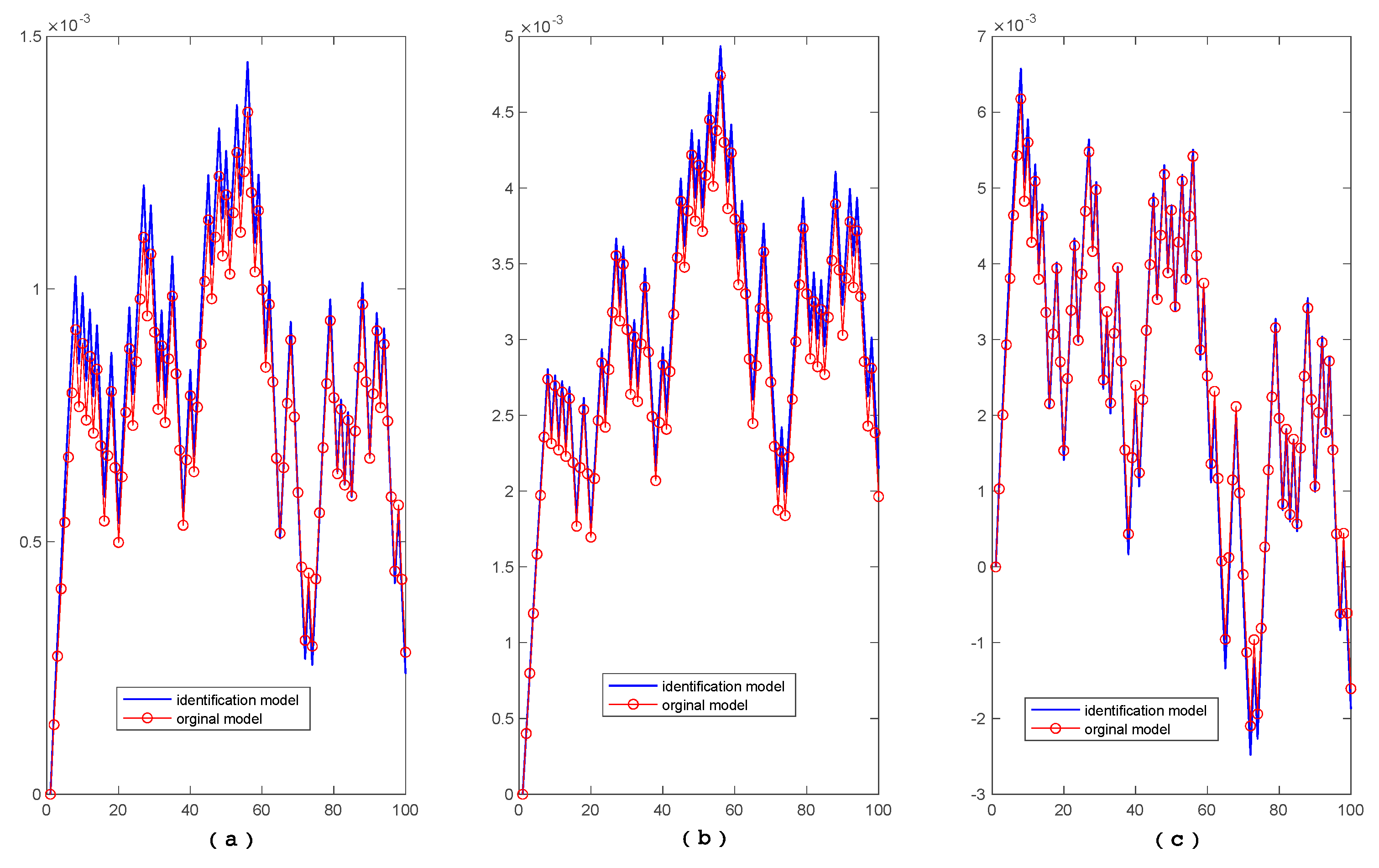
Figure 1 shows the open-loop output of the identification model in three modes in comparison with the output of CSTR.
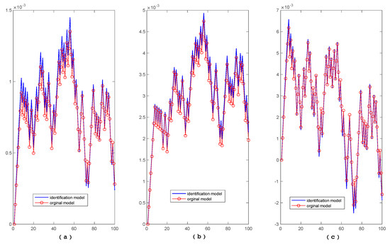
Figure 1.
Open-loop output between the identification model and CSTR. (a) The open-loop output between Mode1 and CSTR. (b) The open-loop output between Mode2 and CSTR. (c) The open-loop output between Mode3 and CSTR.
In Table 1, the order of Mode1 is less than the order of Mode2 that is equal to Mode3. Then, the three models, Mode1, Mode2, and Mode3 form the heterogeneous multiple models of the nonlinear system, the CSTR. When transforming the input–output transfer function into state, mode1 has one state variable, , and mode2 and mode3 have two state variables , thus obtaining three state-space equations as follows:
Define auxiliary state variable for the state space equation of Mode1, then the new state variables of mode1 are , and . With the state variable , the state space equation of mode1 (Equation (26)) can be transformed into the following equation:
Equations (27)–(29) are the multiple model of CSTR. The cost function is given by:
where ,, and .
With Step I to Step VI in the proposed algorithm, the optimal boundary in operating space is evaluated and the decomposition result, , is shown in Figure 2.
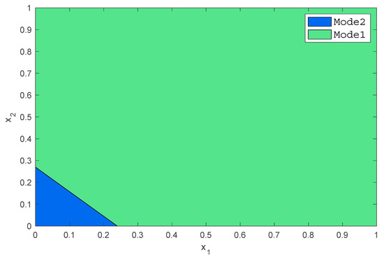
Figure 2.
Boundary condition of operating space obtained with proposed method. , are the state variables of the multiple model.
In Figure 2, only two modes, Mode1 and Mode2, are required for CSTR in the proposed method. Another decomposition method—gap metric—is introduced with which the output space of CSTR is decomposed into three sub-regions, ,, and, as shown in Figure 3 [41].
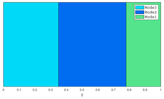
Figure 3.
Boundary condition of operating space with gap-metric method.
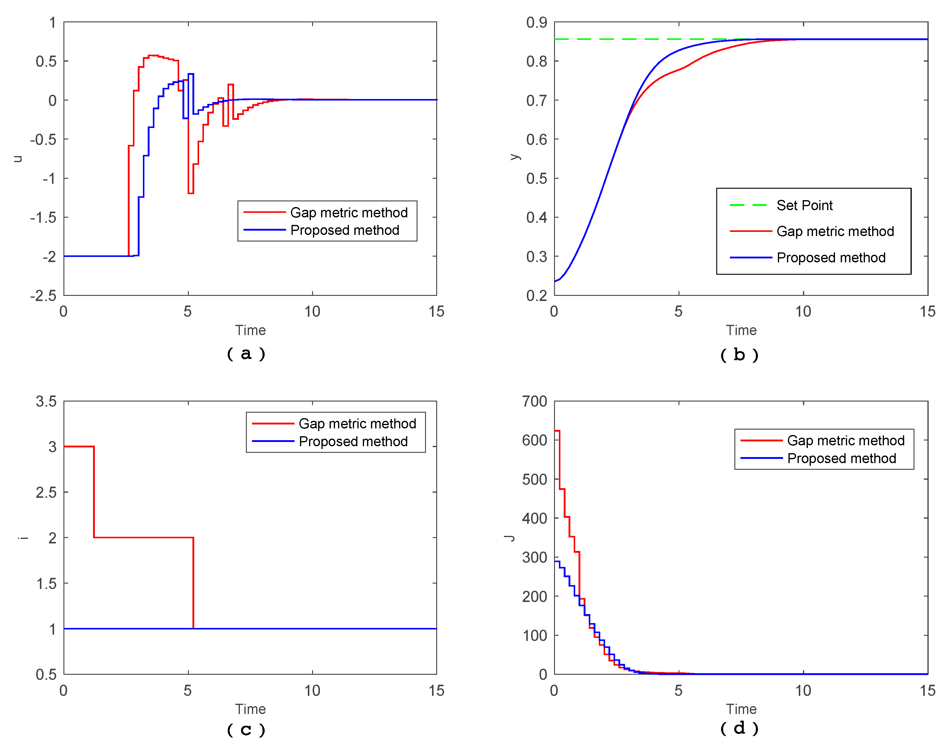
Finally, based on the obtained optimal operating regions and corresponding multiple model, a hybrid-model-based MPC is designed and implemented, where the terminal time , and is the initial point. The trajectories of input u, output y, mode , and objective function value with two methods are presented in Figure 4.
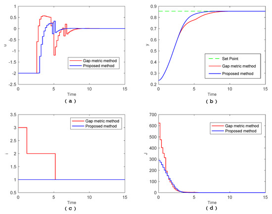
Figure 4.
Simulation profile of multiple model predictive control with two decomposition results. (a) The input u profile of multiple model predictive control with two methods; (b) the output y profile of multiple model predictive control with two methods; (c) the mode i profile of multiple model predictive control with two decomposition results, and (d) the objective function J profile of hybrid-model-based MPC with two methods.
As shown in Figure 4, MPC controllers designed with two methods can operate the CSTR to the set point accurately. From the mode trajectories (Figure 4c), with the gap-based method, we know that the process undergoes three modes, namely, starting at , reaching , and finally at. However, with the proposed method, only is available in the entire operating procedure. From the output profile (Figure 4b), settling time of the CSTR with the proposed method is much faster than with gap-based method. From the control policy profile (Figure 4a), control input jumps more frequently with the gap-based method. Consequently, we can say that only using one mode achieves better system performance than using three modes. From the objective function profile, achieving the optimal objective with the gap-based method requires much more energy than with proposed method.
7. Conclusions
Following our previous work [33,34], which proposed an integrated framework of operating space partition and optimal control of the homogeneous multiple model, this paper proposes a new systematic operating space partition method of the heterogeneous multiple model where the closed loop performance is considered. The heterogeneous multiple model of nonlinear systems is obtained by an identification technique and formulated by an input–output model. Due to optimal control performance being explained in the state space field, the input–output model is transformed into a state space model. With auxiliary variables, the obtained heterogeneous state space model is transformed into a homogeneous multiple model underlying each state having the same physical meaning, and the optimal operating range partition is obtained by optimal boundary conditions in state space. The existing decomposition methods of heterogeneous multiple model approaches are according to the properties of open-loop system dynamics. In contrast, the proposed decomposition method is from the perspective of closed-loop systems performance, thus guaranteeing the overall performance of nonlinear systems.
Future research will include the improvement of computational algorithms derived in this paper, when transforming the heterogeneous multiple model into a homogeneous multiple model may increase the number of state variables of a multiple model and further lead to computational burden in subsequent work.
Author Contributions
Conceptualization, B.W.; Data curation, Y.Y.; Formal analysis, B.W.; Project administration, X.L.; Supervision, X.L.; Validation, Y.Y. All authors have read and agreed to the published version of the manuscript.
Funding
This research received no external funding.
Conflicts of Interest
The authors declare no conflict of interest.
References
- Subramanian, A.S.R.; Adams, T.A. Modeling and simulation of energy systems: A review. Processes 2018, 6, 238. [Google Scholar] [CrossRef]
- Zendehboudi, S.; Rezaei, N.; Lohi, A. Applications of hybrid models in chemical, petroleum, and energy systems: A systematic review. Appl. Energy 2018, 228, 2539–2566. [Google Scholar] [CrossRef]
- Murray-Smith, R.; Johansen, T.A. The operating regime approach to nonlinear modelling and control. In Multiple Model Approaches to Modelling and Control, 1st ed.; Murray-Smith, R., Johansen, T.A., Eds.; Taylor & Francis: London, UK, 1997; Volume 3, pp. 60–78. [Google Scholar]
- Takagi, T.; Sugeno, M. Fuzzy identification of systems and its applications to modeling and control. IEEE Trans. Syst. Man Cybern. 1985, 15, 116–132. [Google Scholar] [CrossRef]
- Xu, J.; Huang, X.L.; Wang, S.N. Adaptive hinging hyperplanes and its applications in dynamic system identification. Automatica 2009, 45, 2325–2332. [Google Scholar] [CrossRef]
- Ferrari-Trecate, G.; Muselli, M.; Liberati, D.; Morari, M. A clustering technique for the identification of piecewise affine systems. Automatica 2003, 39, 205–217. [Google Scholar] [CrossRef]
- Walczak, B.; Massart, D.L. Local modelling with radial basis function networks. Chem. Intell. Lab. Syst. 2000, 50, 179–198. [Google Scholar] [CrossRef]
- Bachnas, A.A.; Tóth, R.; Ludlage, J.H.A.; Mesbah, A. A review on data-driven linear parameter-varying modeling approaches: A high-purity distillation column case study. J. Process Control 2014, 24, 272–285. [Google Scholar] [CrossRef]
- Miranian, A.; Rouzbehi, K. Nonlinear power system load identification using local model networks. IEEE Trans. Power Syst. 2013, 28, 2872–2881. [Google Scholar] [CrossRef]
- Adeniran, A.A.; El Ferik, S. Modeling and identification of nonlinear systems: A review of the multimodel approach—Part 2. IEEE Trans. Syst. Man Cybern. Syst. 2017, 47, 1160–1168. [Google Scholar] [CrossRef]
- Adeniran, A.A.; El Ferik, S. Modeling and identification of nonlinear systems: A review of the multimodel approach—Part 1. IEEE Trans. Syst. Man Cybern. Syst. 2016, 47, 1149–1159. [Google Scholar] [CrossRef]
- Feng, G. A survey on analysis and design of model-based fuzzy control systems. IEEE Trans. Fuzzy Syst. 2006, 14, 676–697. [Google Scholar] [CrossRef]
- Li, X.R.; Bar-Shalom, Y. A recursive multiple model approach to noise identification. IEEE Tran. Aerosp. Electron. Syst. 1994, 30, 671–684. [Google Scholar] [CrossRef]
- Nakada, H.; Takaba, K.; Katayama, T. Identification of piecewise affine systems based on statistical clustering technique. Automatica 2005, 41, 905–913. [Google Scholar] [CrossRef]
- Du, J.; Johansen, T.A. Integrated multimodel control of nonlinear systems based on gap metric and stability margin. Ind. Eng. Chem. Res. 2014, 53, 10206–10215. [Google Scholar] [CrossRef]
- Böling, J.M.; Seborg, D.E.; Hespanha, J.P. Multi-model adaptive control of a simulated pH neutralization process. Control Eng. Pract. 2007, 15, 663–672. [Google Scholar] [CrossRef]
- Song, C.; Wu, B.; Li, P. A hybrid model-based optimal control method for nonlinear systems using simultaneous dynamic optimization strategies. J. Process Control 2012, 22, 852–860. [Google Scholar] [CrossRef]
- Xu, D.; Jiang, B.; Shi, P. Nonlinear actuator fault estimation observer: An inverse system approach via a T–S fuzzy model. Int. J. Appl. Math. Comput. Sci. 2012, 22, 183–196. [Google Scholar] [CrossRef]
- Narendra, K.S.; Wang, Y.; Mukhopadhay, S. Fast Reinforcement Learning using multiple models. In Proceedings of the IEEE 55th Conference on Decision and Control (CDC), Las Vegas, NV, USA, 12–14 December 2016; pp. 7183–7188. [Google Scholar]
- Angelov, P.P.; Gu, X.; Príncipe, J.C. Autonomous Learning Multimodel Systems from Data Streams. IEEE Trans. Fuzzy Syst. 2017, 26, 2213–2224. [Google Scholar] [CrossRef]
- Ru, J.; Li, X.R. Variable-structure multiple-model approach to fault detection, identification, and estimation. IEEE Trans. Control Syst. Technol. 2008, 16, 1029–1038. [Google Scholar] [CrossRef]
- Orjuela, R.; Marx, B.; Ragot, J.; Maquin, D. Nonlinear system identification using heterogeneous multiple models. Int. J. Appl. Math. Comput. Sci. 2013, 23, 1–13. [Google Scholar] [CrossRef]
- Filev, D. Fuzzy modeling of complex systems. Int. J. Approx. Reason. 1991, 5, 281–290. [Google Scholar] [CrossRef]
- Gawthrop, P.J. Continuous-time local state local model networks. In Proceedings of the IEEE International Conference on Systems, Man and Cybernetics. Intelligent Systems for the 21st Century, Vancouver, BC, Canada, 22–25 October 1995; Volume 1, pp. 852–857. [Google Scholar]
- Venkat, A.N.; Vijaysai, P.; Gudi, R.D. Identification of complex nonlinear processes based on fuzzy decomposition of the steady state space. J. Process Control 2003, 13, 473–488. [Google Scholar] [CrossRef]
- Gregorcic, G.; Lightbody, G. Nonlinear system identification: From multiple-model networks to Gaussian processes. Eng. Appl. Artif. Intell. 2008, 21, 1035–1055. [Google Scholar] [CrossRef]
- Kanev, S.; Verhaegen, M. Multiple model weight estimation for models with no common state. In Proceedings of the 6th IFAC Symposium on Fault Detection, Supervision and Safety of Technical Processes, Beijing, China, 30 August–1 September 2006; pp. 637–642. [Google Scholar]
- Uppal, F.J.; Patton, R.J.; Witczak, M. A neuro-fuzzy multiple-model observer approach to robust fault diagnosis based on the DAMADICS benchmark problem. Control Eng. Pract. 2006, 14, 699–717. [Google Scholar] [CrossRef]
- Orjuela, R.; Marx, B.; Ragot, J.; Maquin, D. On the simultaneous state and unknown inputs estimation of complex systems via a multiple model strategy. IET Control Theory Appl. 2009, 3, 877–890. [Google Scholar] [CrossRef]
- Gao, Y.; Liu, Y.; Li, X.R.; Jilkov, V.P. Multiple-model estimation with heterogeneous state representation. In Proceedings of the 2015 18th International Conference on Information Fusion (Fusion), Washington, DC, USA, 6–9 July 2015; pp. 1840–1847. [Google Scholar]
- Ben Atia, S.; Messaoud, A.; Ben Abdennour, R. An online identification algorithm of unknown time-varying delay and internal multimodel control for discrete non-linear systems. Mat. Comput. Modell. Dyn. Syst. 2018, 24, 26–43. [Google Scholar] [CrossRef]
- Du, J.J.; Song, C.Y.; Li, P. Multimodel control of nonlinear systems: An integrated design procedure based on gap metric and H∞ loop shaping. Ind. Eng. Chem. Res. 2012, 51, 3722–3731. [Google Scholar] [CrossRef]
- Nikolaou, M.; Misra, P. Linear control of nonlinear processes: Recent developments and future directions. Comput. Chem. Eng. 2003, 27, 1043–1059. [Google Scholar] [CrossRef]
- Du, J.J.; Johansen, T.A. Control-relevant nonlinearity measure and integrated multi-model control. J. Process Control 2017, 57, 127–139. [Google Scholar] [CrossRef]
- Song, C.Y.; Wu, B.; Zhao, J.; Li, P. An integrated state space partition and optimal control method of multi-model for nonlinear systems based on hybrid systems. J. Process Control 2015, 25, 59–69. [Google Scholar] [CrossRef]
- Song, C.Y.; Wu, B.; Zhao, J. An integrated output space partition and optimal control method of multiple-model for nonlinear systems. Comput. Chem. Eng. 2018, 113, 32–43. [Google Scholar] [CrossRef]
- Song, C.Y.; Li, P. Near optimal control for a class of stochastic hybrid systems. Automatica 2010, 46, 1553–1557. [Google Scholar] [CrossRef]
- Kushner, H.J.; Dupuis, P.G. Numerical Methods for Stochastic Control Problems in Continuous Time, 2nd ed.; Springer: Berlin, NY, USA, 2002; pp. 1240–1351. [Google Scholar]
- Mayne, D.Q. Model predictive control: Recent developments and future promise. Automatica 2014, 50, 2967–2986. [Google Scholar] [CrossRef]
- Bemporad, A.; Morari, M. Control of systems integrating logic, dynamics, and constraints. Automatica 1999, 35, 407–427. [Google Scholar] [CrossRef]
- Du, J.J.; Song, C.; Li, P. Application of gap metric to model bank determination in multilinear model approach. J. Process Control 2009, 19, 231–240. [Google Scholar] [CrossRef]
© 2020 by the authors. Licensee MDPI, Basel, Switzerland. This article is an open access article distributed under the terms and conditions of the Creative Commons Attribution (CC BY) license (http://creativecommons.org/licenses/by/4.0/).

