Abstract
In large scale ships, the most used controllers for the steam/water loop are still the proportional-integral-derivative (PID) controllers. However, the tuning rules for the PID parameters are based on empirical knowledge and the performance for the loops is not satisfying. In order to improve the control performance of the steam/water loop, the application of a recently developed PID autotuning method is studied. Firstly, a ‘forbidden region’ on the Nyquist plane can be obtained based on user-defined performance requirements such as robustness or gain margin and phase margin. Secondly, the dynamic of the system can be obtained with a sine test around the operation point. Finally, the PID controller’s parameters can be obtained by locating the frequency response of the controlled system at the edge of the ‘forbidden region’. To verify the effectiveness of the new PID autotuning method, comparisons are presented with other PID autotuning methods, as well as the model predictive control. The results show the superiority of the new PID autotuning method.
1. Introduction
The steam/water loop in a steam power plant is the process that provides water for the boiler and recycles the waste steam from the turbine [1]. Due to the harsh operation environment, the system of steam/water loop in large ships suffers more disturbances than the equipment installed in onshore power stations. The steam/water loop is a system with multiple variables and strong interactions. All above become obstacles to obtain satisfying system performance for the steam/water loop in large scale ships.
The sub-loops in the steam/water loop are listed as follows—the control loop for drum water level, the control loop for exhaust manifold pressure, the control loop for deaerator pressure, the control loop for deaerator water level and the control loop for condenser water level. The main difficulties existing in the system can be summarized as follows:
- when the water turns between steam and liquid, the false water level phenomenon appears for reason of the shrink and swell in the water, which makes the drum water level control loop a non-minimum phase system [2].
- the water in the condenser goes to the deaerator, hence, strong interactions exist in the water control loops of the deaerator and the condenser.
- the steam required in the deaerator is from the exhaust manifold, which leads to strong coupling in the pressure control loops of the deaerator and exhaust manifold.
- the amount of required steam in the deaerator changes with the feedwater flow rate. Hence, the water level and the pressure are two strong coupling variables in the deaerator.
For the false water level phenomenon, the most used method in reality is the cascade-three elements control [3,4,5], which can be treated as a hybrid structure consisting of feedback control and feed-forward control. The water level is the feedback signal, while the feed-forward signals are chosen as steam flow rate and water flow rate. Besides, many advanced control strategies have been studied on the drum water level control in literature, including the sliding mode control [6,7,8], model predictive control [9,10,11,12,13], backstepping control [14,15] and adaptive disturbance rejection control (ADRC) [16,17].
In Reference [8], a robust adaptive sliding mode controller was designed for the boiler-turbine unit to deal with the unknown bounded uncertainties and external disturbances. The effectiveness was evaluated comparing with a type-I servo controller. Liu proposed a coordinated control with two nonlinear model predictive control methods for a steam-boiler generation plant [11]. One of the models was obtained with input-output feedback linearization technique. The other model was obtained with neuro-fuzzy networks, which is a nonlinear dynamic model. An economic model predictive controller was proposed, and the part of the cost function is composed of the economic index [9]. To guarantee the stability, stable Sontag controller and corresponding region were designed. A backstepping procedure was implemented to adapt the unknown parameters in a power plant station, in which the nonlinearity of the system is synthesized. Meanwhile, the control law was obtained with symbolic computations [15]. Sun applied the ADRC algorithm to a power plant. For system safety, an automatic tuning tool was designed when the ADRC was applied to the loop [17].
For the coupling issue between the water level control loops in deaerator and condenser, a fuzzy PID algorithm was proposed for a multi-variable control system, which has been applied in practice in the Yangzhou thermal power plant [18]. Other work shows in Reference [19], in which the system is decoupled firstly, and a PID neural network was designed for the system. According to experience, the initial weighting factors and learning coefficients were selected, and the convergence of the proposed method was enhanced.
The deaerator is used to remove the oxygen and other gas dissolved in feed water. When there is a change in the deaerator water level, the pressure changes a lot for the interactions between the two variables. Liao proposed a self-tuning fuzzy PID controller, in which the overshoot was decreased from 40% to 12% [20]. Wang applied the decoupling method to the deaeration system [21]. Then, the neurons for proportional, integral and derivative were obtained with a PID neural network and the superiority was validated for the PID neural network.
The exhaust manifold has the following functions—recycles waste steam from turbine and auxiliary machines and supplies steam for the deaerator. Hence, the exhaust manifold pressure has strong interaction with the deaerator pressure. For the modeling of the exhaust manifold pressure, a mean-value model was derived with the compressible flow equation, in which the exhaust system was treated as a fixed-geometry restriction between the exhaust manifold and the outlet of the tailpipe [22]. A generic model was used for the controller design [23]. In this method, the exhaust gas flow was estimated with an observer, which comes from the loops with high pressure or low pressure. Then, an intake burnt gas fraction control was designed to obtain satisfying performance for a LTC-Diesel engine.
For the loop control of multiple interacting subsystems, a practical tuning method was proposed with model based predictive control and it is validated that the method is suitable for manually tuning for predictive control [24]. Linear and nonlinear PID controllers were designed for a twin rotor MIMO system and based on nonlinear-segmented observers, the parameters for nonlinear PID controller were obtained. The results showed the superiority of the nonlinear PID [25]. Based on fractional order method, designing controller with adaptive laws was proposed [26]. To deal with the interactions between sub-loops in a process, a theoretical framework was proposed, which is useful for controller design problems [27]. An optimization method was proposed to make a trade-off between implementation cost and achievable performance for multiple interacting subsystems [28]. In order to optimize the choice of the cost function and their effect to the overall system performance, strategy for selection of the optimal criteria according to context conditions was proposed and a windmill park experiment was conducted to validate the performance [29].
In most of the methods mentioned above, an accurate model is necessary for the controller design. However, according to Reference [30], the expenses of time in the procedure of modeling takes 60%–70% of the total time for a controller design. Moreover, the steam/water loop is a complex system, and a model for the entire system is difficult to be obtained [31]. In the industrial process control, the most used strategy is still PID controller. The PID controllers play an important role in process control [32,33,34,35]. Meanwhile, 60% of loops have bad performance and 25% can not meet the performance requirements in industry [36]. In order to develop much advanced tuning method for the PID controller, an universal direct tuner was proposed for loop control [37]. In this paper, a PID autotuner—named the KC autotuning method—is applied to the steam/water loop in large scale ships. According to the user-defined requirement, a ‘forbidden region’ can be plotted on the Nyquist plane. Then, the dynamic of the system around the operating point can be obtained with a simple sine test. By designing a proper PID controller, the system’s frequency response can be tangent to the ‘forbidden region’, where the requirements can be fulfilled.
The paper is structured as follows—firstly, the steam/water loop in large scale ships is introduced in Section 2. Then, the detailed theory of the KC autotuner is presented in Section 3. In Section 4, other PID autotuning methods are listed. The comparison experiments are conducted in Section 5 and the results are analyzed. The conclusions are shown in Section 6.
2. Introduction of the Steam/Water Loop
There are four main pieces of equipment in the steam/water loop, including the drum, exhaust manifold, deaerator and condenser, as shown in Figure 1. In system, the red line is the steam loop, while the green line indicates the water loop. The steam/water loop works as follows—firstly, the feed water gets pre-heated in the economizer and pumped into the drum. Then, the feedwater goes to the mud drum for its high density. After absorbing heat from the risers, the water becomes a mixture of water and steam. Thirdly, the steam gets separated in the drum and heated in the superheater, after which the steam is qualified to serve in turbine. Fourthly, the waste steam from the turbine and other auxiliary machines goes to the exhaust manifold. The waste steam is mostly used for condensation in the condenser and the remaining part goes to the deaerator for deoxygenation. Finally, the condensed water goes to the deaerator. After being deoxygenated, the water will be pumped to the drum to work again.
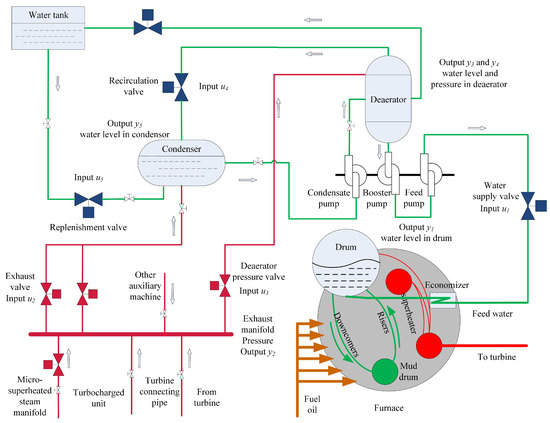
Figure 1.
Scheme of steam/water loop [38] (reproduced with permission from Zhao, S.; Maxim, A.; Liu, S.; De Keyser, R.; and Ionescu, C, Processes; published by MDPI, 2018).
The manipulated variables are the positions of the valves that control the flow rates of feedwater into the drum (), exhaust steam out of the exhaust manifold (), exhaust steam into the deaerator (), water from the deaerator () and water into the condenser (), respectively. The controlled output variables are the values of the water level in drum (), pressure in exhaust manifold (), water level () and pressure () in deaerator, and water level of condenser (), respectively [31]. Equation (1) shows the transfer function of the system around the operation points shown in Table 1. The constraints of the system can be found in Equation (2).
where , , , , , , , , and other transfer functions .

Table 1.
System operating points and range.
The inputs are normalized in percentage values of the valve opening, and 0 means the valve is closed completely and 1 means the valve is opened fully. Additionally, the unit for input rates is measured in opening degree per second.
3. Detailed Theory of KC Autotuning Method
In this section, the theory of the KC autotuning method is introduced in detail [39,40,41,42]. The main idea of the KC autotuner is shown in Figure 2. By designing a PID controller indicated with , the point B on the Nyquist curve of process can be placed at the point A of the loop . Circle 2 in Figure 2 indicates the ‘forbidden region’ obtained according to user defined performance such as robustness or phase and gain margin. In this paper, the performance of phase margin and gain margin are chosen, and a similar theory can be obtained with robustness. In order to fulfill the performance requirement, the loop should be tangential to the ‘forbidden region’ on the Nyquist plane, which means that the slopes should be the same of the loop as well as the ‘forbidden region’ on the edge of the region.
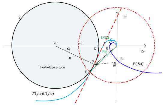
Figure 2.
Graphic illustration of the KC autotuning principle [43] (reproduced with permission from Zhao, S.; Ionescu, C.M.; De Keyser, R.; and Liu, S. In 3rd IFAC Conference in Advances in Proportional-Integral-Derivative Control; published by Elsevier, 2018).
The procedure for KC autotuning can be summarized as follows:
- (1)
- Obtain the critical frequency of the system ( is usually critical frequency, but might be different);
- (2)
- Conduct sine tests around the operating points on the steam/water loop;
- (3)
- According to the loop margin requirements, calculate a ‘forbidden region’ on the Nyquist plane;
- (4)
- Calculate parameters for the PID controller for the points on the region edge (for from to );
- (5)
- Search for the point, where the slope of the loop is the same with the slope of the ‘forbidden region’;
- (6)
- The parameters for the PID controller are obtained from step 5).
3.1. Slope of the ‘Forbidden Region’
According to loop margin requirements, points D and E can be obtained in Figure 2. D indicates the intersection of gain margin with negative real axis. E is the intersection of phase margin with unit circle. With D and E, the ‘forbidden region’ can be calculated as:
where the and are the real part and image part of the points on the circle 2; and are user defined phase margin and gain margin of the system.
Then the center C and the radius R of the ‘forbidden region’ are as follows:
The slope at point A gives:
3.2. Slope of the Loop
The slope of loop is obtained according to the derivative of .
with the specified frequency.
The gain and phase at point A can be obtained as:
It can be re-written as:
3.2.1. Calculation for and Its Derivation
The following section introduces how to obtain the parts of and . The typical form of the PID controller gives:
where , are the proportional gain, integration time constant and differential time constant, respectively.
According to the ‘forbidden region’, the modulus and phase are as follows:
Hence, we have
Let:
Taking the relationship of , the at the frequency can be calculated as:
Substitute to Equation (9) and gives:
The items of and are obtained as follows:
3.2.2. Calculation for and Its Derivation
The following introduces how to get the parts of and its derivation . In order to obtain the magnitude and phase slope of the process at the gain crossover frequency, a sinusoidal input signal around the operation point is imposed into the system:
where is the amplitude of the sinusoidal signal and denotes the input operation point.
Then there will be another sinusoidal signal in the output of the system, which can be described as:
where , indicate the amplitude and phase of the output signal, and is the output operation point.
Hence, the part can be obtained as:
with , and .
According to the property of Laplace-transform:
We can conclude that, when there is an input applied to the process , the Laplace transform of the output gives:
which can be re-written as:
Considering , where the and are the Laplace transforms of input and output, if the signal is imposed to the process , the corresponding output will be , yielding:
Furthermore, the following equation can be obtained:
where indicates the output of the process derivative.
Hence, the output of the process derivative can be calculated as:
According to Equation (29), the experimental scheme to apply the sine signal to the system can be obtained as shown in Figure 3.
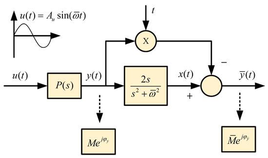
Figure 3.
The scheme of sine test to obtain the knowledge of the process around the operating point [39] (reproduced with permission from De Keyser, R., Muresan, C. I. and Ionescu, C. M. A novel auto-tuning method for fractional order PI/PD controllers. ISA transactions, published by Elsevier, 2016).
The modulus and phase of the process can be obtained by measuring the output :
with . and are the amplitude and phase of the signal , respectively.
Now, the four parts , , and are all obtained for Equation (7).
For , find the which minimizes , that is,
Then the PID parameters can be calculated as:
3.3. Application to Mimo System
In order to apply the KC autotuning method based PID controller to a Multi-Input and Multi-Output (MIMO) system, the following procedure is required to be performed on the system.
- (1)
- Apply sine test around the operating points on one of the sub-loops, while keeping other sub-loops to work at their own operating points. And the controller parameters can be calculated for the selected loop, with the magnitude and phase obtained from the sine test;
- (2)
- Keep the previous sub-loop working at its operating point with the obtained PID control, and conduct a new sine test on one the other sub-loops. The magnitude and phase can be obtained for the new sub-loop and the controller can be calculated;
- (3)
- Repeat step 2 for each sub-loop until the output magnitude and phase do not change significantly between consecutive tests.
- (4)
- The parameters for the PID controller can be obtained for all the sub-loops after step 3 is completed.
4. A Brief Introduction of Other PID Autotuners
To validate the KC autotuning method, comparisons are conducted with other PID autotuning methods, including Åström-Hägglund (AH) [44], Phase Margin (PM) and Kaiser-Rajka (KR) methods. The brief introduction for the PID autotuners are as follows.
These methods are based on a relay test shown in Figure 4. The output will oscillate around the system’s operation point with a relay excitation signal. After a period of time, the oscillation will be a steady periodic signal with amplitude and critical period . A typical result for a relay test can be find in Figure 5.
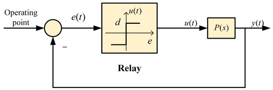
Figure 4.
Schematic representation of the relay test.
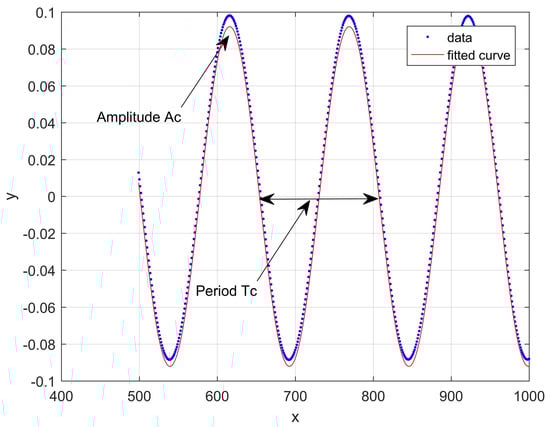
Figure 5.
Typical result of the relay test.
The critical gain can be obtained as:
The PID parameters obtained based on the AH and PM method are:
The PID parameters based on the KR method are obtained with a relay plus delay test and the scheme is shown in Figure 6. The delay time is set as , with the and the desired phase margin and critical period.
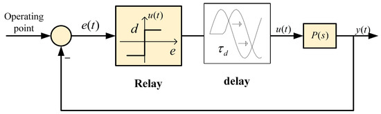
Figure 6.
Schematic representation of the relay plus delay test.
The PID parameters obtained for the KR method are:
where ; and are the amplitude and period of the result in the relay plus delay test.
5. Experiments and Results Analyses
5.1. A Simple Single Input Single Output System Example
In this section, the test on a simple single input single output (SISO) system example is provided to verify the effectiveness of the KC PID autotuning method. The transfer function of the SISO system is shown as follows:
In the SISO system test, the performance for reference tracking and disturbance rejection are verified for the KC method. The PID parameters obtained with AH, PM, KR and KC methods are shown in Table 2.
Table 2.
PID parameters with different autotuners for the single input single output (SISO) system.
The results are shown in Figure 7. It is obvious that the KC method has the best performance compared with other PID autotuning methods, not only in reference tracking, but also in disturbance rejection. In the KC method, the performance requirements, such as robustness or phase margin and gain margin, are obtained by locating the frequency response of the process to be tangential to the boundary of the ‘forbidden region’. Hence, the PID parameters obtained with the KC method are less conservative compared with other PID autotuning methods, which leads to a fast dynamic response in the KC method. and are introduced for the PID controller design.
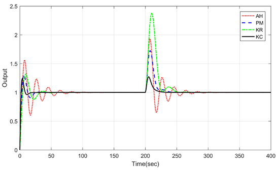
Figure 7.
The results of a SISO system with different PID autotuners.
5.2. Simulation on Steam/Water Loop in Large Scale Ships
In the experiments, step signals are introduced to the system at different times. Table 3 shows the step setpoints changing. Table 1 is the initial condition of the steam/water loop. and are introduced for the PID controller design.
Table 3.
Setpoints for different loops in the experiments.
The parameters obtained with different PID autotuners are shown in Table 4. Loop 1 to loop 5 are the control loops for drum water, exhaust manifold pressure, deaerator pressure, deaerator water level and condenser water level, respectively.
Table 4.
PID parameters with different autotuners for steam/water loop.
The simulation results are shown in Figure 8. The performance is evaluated with the following definitions, including the Integrated Absolute Relative Error (), Integral Secondary control output (), Ratio of Integrated Absolute Relative Error (), Ratio of Integral Secondary control output () and combined index (J). The results for the performance indexes are listed in Table 5 and Table 6.
where is the steady state value of ith input; , are the two compared controllers; the weighting factors and in Equation (47) are chosen as .
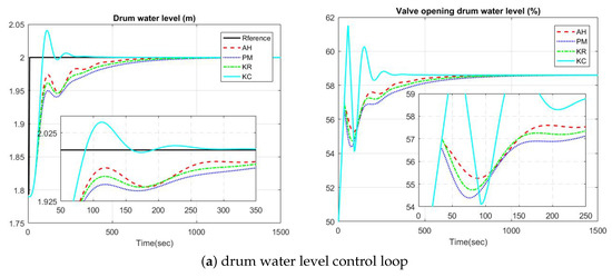
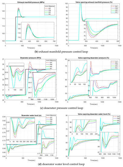
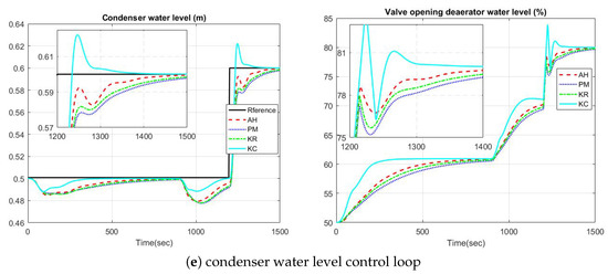
Figure 8.
Outputs of the steam/water loop with different PID autotuning methods (The outputs are listed on the left and the inputs are listed on the right).
Table 5.
Performance indexes for and .
As shown in Figure 8 and Table 6, the KC autotuner has the best performance compared to other PID autotuners. In Table 6, the KC method has a worse performance only in loop 3, which is because of the strong interaction between deaerator water level indicated by loop 3 and deaerator pressure indicated by loop 4. In order to obtain good performance for loop 4, the valve opening for the deaerator water level changes a lot, which also has a noticeable negative effect on loop 3. In order to test the performance of the KC autotuner with a model based controller, a comparison between the KC autotuning based PID controller and Model Predictive Controller (MPC) is conducted. The results are shown in Figure 9. The detailed parameters for the MPC can be found in Reference [31].
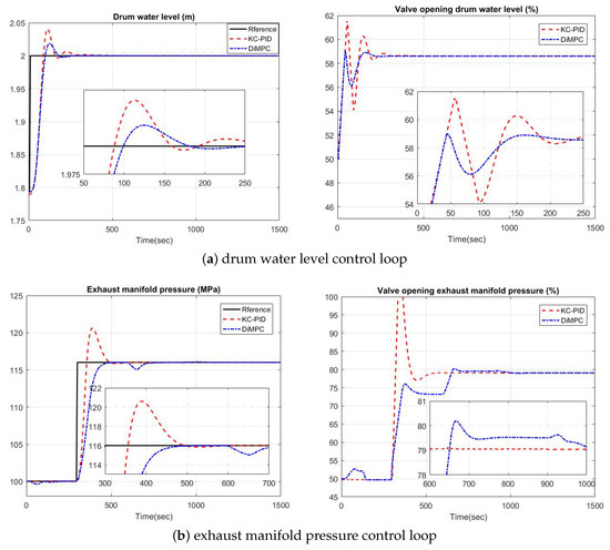
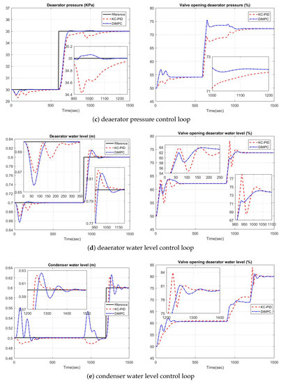
Figure 9.
Outputs of the steam/water loop with KC based PID controller and MPC (The outputs are listed on the left, and the inputs are listed on the right).
According to the results shown in Figure 9, both methods provide satisfying results for the steam/water loop, and obviously the MPC controller provides better results than the PID controller based on the KC autotuning method. However, a good model for the system is essential for the MPC, which is not necessary in the PID controller with the KC autotuning method.
6. Conclusions
In the steam/water loop of large scale ships, the PID controller is still the most applied control strategy. However, the tuning results for the PID controllers are not satisfying. In this paper, the parameters for a PID controller are tuned with a recently developed method named KC autotuner, which is free to the system model. According to the user-defined system performance, a ‘forbidden region’ is obtained on the Nyquist plane. Through sine tests performed on the steam/water loop, the dynamics around the operating points are obtained. By designing a proper PID controller, the loop frequency response of the controlled system can be tangent to the ‘forbidden region’, which guarantees the system performance requirements. The comparison results show the superiority of the KC method.
Author Contributions
Methodology, R.D.K., C.-M.I. and S.Z.; software, S.Z. and S.L.; formal analysis, S.Z.; writing—original draft preparation, S.Z.; writing—review and editing, S.Z., R.D.K., S.L., and C.-M.I.; supervision, C.-M.I., S.L. and R.D.K.; funding acquisition, S.Z., S.L. and C.-M.I. All authors have read and agreed to the published version of the manuscript.
Funding
Part of this project is funded by a special research fund of Ghent University, MIMOPREC STG020-18 (Ionescu), National Natural Science Foundation of China subsidization project (51579047), the Doctoral Scientific Research Foundation of Heilongjiang (No. LBH-Q14040), the Fundamental Research Funds for the Central Universities under grant 3072019CF0408, 3072019CFT0403.
Acknowledgments
Shiquan Zhao acknowledges the financial support from Chinese Scholarship Council (CSC) under grant 201706680021 and the Co-funding for Chinese PhD candidates from Ghent University under grant 01SC1918.
Conflicts of Interest
The authors declare no conflict of interest.
References
- Drbal, L.; Westra, K.; Boston, P. Power Plant Engineering; Springer Science & Business Media: Berlin, Germany, 2012. [Google Scholar]
- Åström, K.J.; Bell, R.D. Drum-boiler dynamics. Automatica 2000, 36, 363–378. [Google Scholar] [CrossRef]
- Xia, Y.; Liu, B.; Fu, M. Active disturbance rejection control for power plant with a single loop. Asian J. Control 2012, 14, 239–250. [Google Scholar] [CrossRef]
- Yu, N.; Ma, W.; Su, M. Application of adaptive Grey predictor based algorithm to boiler drum level control. Energy Convers. Manag. 2006, 47, 2999–3007. [Google Scholar] [CrossRef]
- Cheng, Q.M.; Zheng, Y.; Du, X. Three-element Drum Water-level Cascade Control System Featuring a Self-disturbance-resistant Controller. J. Eng. Therm. Energy Power 2008, 23, 69. [Google Scholar]
- Moradi, H.; Saffar-Avval, M.; Bakhtiari-Nejad, F. Sliding mode control of drum water level in an industrial boiler unit with time varying parameters: A comparison with H∞-robust control approach. J. Process Control 2012, 22, 1844–1855. [Google Scholar] [CrossRef]
- Aliakbari, S.; Ayati, M.; Osman, J.H.; Sam, Y.M. Second-order sliding mode fault-tolerant control of heat recovery steam generator boiler in combined cycle power plants. Appl. Therm. Eng. 2013, 50, 1326–1338. [Google Scholar] [CrossRef]
- Ghabraei, S.; Moradi, H.; Vossoughi, G. Multivariable robust adaptive sliding mode control of an industrial boiler–turbine in the presence of modeling imprecisions and external disturbances: A comparison with type-I servo controller. ISA Trans. 2015, 58, 398–408. [Google Scholar] [CrossRef]
- Liu, X.; Cui, J. Economic model predictive control of boiler-turbine system. J. Process Control 2018, 66, 59–67. [Google Scholar] [CrossRef]
- Liu, X.; Kong, X. Nonlinear fuzzy model predictive iterative learning control for drum-type boiler–turbine system. J. Process Control 2013, 23, 1023–1040. [Google Scholar] [CrossRef]
- Liu, X.; Guan, P.; Chan, C. Nonlinear multivariable power plant coordinate control by constrained predictive scheme. IEEE Trans. Control Syst. Technol. 2009, 18, 1116–1125. [Google Scholar] [CrossRef]
- Wu, X.; Shen, J.; Li, Y.; Lee, K.Y. Fuzzy modeling and predictive control of superheater steam temperature for power plant. ISA Trans. 2015, 56, 241–251. [Google Scholar] [CrossRef] [PubMed]
- Zhao, S.; Cajo, R.; De Keyser, R.; Liu, S.; Ionescu, C.M. Nonlinear predictive control applied to steam/water loop in large scale ships. In Proceedings of the 12th IFAC Symposium on Dynamics and Control of Process Systems, including Biosystems, Florianópolis, Brazil, 23–26 April 2019; pp. 868–873. [Google Scholar]
- Wei, L.; Fang, F.; Shi, Y. Adaptive backstepping-based composite nonlinear feedback water level control for the nuclear U-tube steam generator. IEEE Trans. Control Syst. Technol. 2013, 22, 369–377. [Google Scholar] [CrossRef]
- Bolek, W.; Sasiadek, J.; Wisniewski, T. Adaptive backstepping control of a power plant station model. IFAC Proc. Vol. 2002, 35, 215–220. [Google Scholar] [CrossRef]
- Sun, L.; Hua, Q.; Shen, J.; Xue, Y.; Li, D.; Lee, K.Y. Multi-objective optimization for advanced superheater steam temperature control in a 300 MW power plant. Appl. Energy 2017, 208, 592–606. [Google Scholar] [CrossRef]
- Sun, L.; Li, D.; Hu, K.; Lee, K.Y.; Pan, F. On tuning and practical implementation of active disturbance rejection controller: A case study from a regenerative heater in a 1000 MW power plant. Ind. Eng. Chem. Res. 2016, 55, 6686–6695. [Google Scholar] [CrossRef]
- Lu, J.; Chen, L.; Zhao, S.; Wu, Y. Multivariable Fuzzy PID Control System for Deaerator’s and Condenser’s Levels in a Thermal Powerunit. Cybern. Syst. 2002, 33, 483–506. [Google Scholar]
- Wang, P.; Meng, H.; Dong, P.; Dai, R.-H. Decoupling control based on PID neural network for deaerator and condenser water level control system. In Proceedings of the 2015 34th Chinese Control Conference (CCC), Hangzhou, China, 28–30 July 2015; pp. 3441–3446. [Google Scholar]
- Liao, Y.F.; Guo, S.D.; Yang, G.; Ma, X.Q. Fuzzy Control of Deaerator Water-Level in Nuclear Power Station Based on MATLAB/Simulink. Appl. Mech. Mater. 2013, 291, 2397–2402. [Google Scholar] [CrossRef]
- Wang, P.; Meng, H.; Ji, Q.Z. Application of PID neural network decoupling control in deaerator pressure and deaerator water level control system. In Asian Simulation Conference; Springer: Berlin/Heidelberg, Germany, 2014; pp. 15–25. [Google Scholar]
- Olin, P.M. A Mean-Value Model for Estimating Exhaust Manifold Pressure in Production Engine Applications; Technical Report, SAE Technical Paper; IEEE: San Francisco, CA, USA, 2008. [Google Scholar]
- Grondin, O.; Moulin, P.; Chauvin, J. Control of a turbocharged diesel engine fitted with high pressure and low pressure exhaust gas recirculation systems. In Proceedings of the 48h IEEE Conference on Decision and Control (CDC) held jointly with 2009 28th Chinese Control Conference, Shanghai, China, 15–18 December 2009; pp. 6582–6589. [Google Scholar]
- Ionescu, C.M.; Copot, D. Hands-on MPC tuning for industrial applications. Bull. Pol. Acad. Sci. Tech. Sci. 2019, 67, 925–945. [Google Scholar]
- Cajo, R.; Agila, W. Evaluation of algorithms for linear and nonlinear PID control for Twin Rotor MIMO System. In Proceedings of the 2015 Asia-Pacific Conference on Computer Aided System Engineering, Quito, Ecuador, 14–16 July 2015; pp. 214–219. [Google Scholar]
- Copot, D.; Ghita, M.; Ionescu, C.M. Simple Alternatives to PID-Type Control for Processes with Variable Time-Delay. Processes 2019, 7, 146. [Google Scholar] [CrossRef]
- Maxim, A.; Ferracuti, R.; Ionescu, C.M. A Theoretical Framework to Determine RHP Zero Dynamics in Sequential Interacting Sub-Systems. Algorithms 2019, 12, 102. [Google Scholar] [CrossRef]
- Haemers, M.; Derammelaere, S.; Rosich, A.; Ionescu, C.M.; Stockman, K. Towards a generic optimal co-design of hardware architecture and control configuration for interacting subsystems. Mechatronics 2019, 63, 102275. [Google Scholar] [CrossRef]
- Ionescu, C.M.; Caruntu, C.F.; Cajo, R.; Ghita, M.; Crevecoeur, G.; Copot, C. Multi-Objective Predictive Control Optimization with Varying Term Objectives: A Wind Farm Case Study. Processes 2019, 7, 778. [Google Scholar] [CrossRef]
- Starr, K.D. Single Loop Control Methods, 1st ed.; ABB Inc.: Westerville, OH, USA, 2015. [Google Scholar]
- Zhao, S.; Maxim, A.; Liu, S.; De Keyser, R.; Ionescu, C.M. Distributed model predictive control of steam/water loop in large scale ships. Processes 2019, 7, 442. [Google Scholar] [CrossRef]
- Samad, T. A survey on industry impact and challenges thereof [technical activities]. IEEE Control Syst. Mag. 2017, 37, 17–18. [Google Scholar]
- Wu, Z.; Li, D.; Xue, Y. A New PID Controller Design with Constraints on Relative Delay Margin for First-Order Plus Dead-Time Systems. Processes 2019, 7, 713. [Google Scholar] [CrossRef]
- Cajo, R.; Zhao, S.; Ionescu, C.M.; De Keyser, R.; Plaza, D.; Liu, S. IMC based PID control applied to the Benchmark PID 18. In Proceedings of the 3rd IFAC Conference in Advances in Proportional-Integral-Derivative Control, Ghent, Belgium, 9–11 May 2018; pp. 728–732. [Google Scholar]
- Zhao, S.; Cajo, R.; Ionescu, C.M.; De Keyser, R.; Liu, S.; Plaza, D. A Robust PID Autotuning Method Applied to the Benchmark PID18. In Proceedings of the 3rd IFAC Conference in Advances in Proportional-Integral-Derivative Control, Ghent, Belgium, 9–11 May 2018; pp. 521–526. [Google Scholar]
- De Keyser, R.; Ionescu, C.M.; Muresan, C.I. Comparative evaluation of a novel principle for PID autotuning. In Proceedings of the 2017 11th Asian Control Conference (ASCC), Gold Coast, QLD, Australia, 17–20 December 2017; pp. 1164–1169. [Google Scholar]
- De Keyser, R.; Muresan, C.I.; Ionescu, C.M. Universal direct tuner for loop control in industry. IEEE Access 2019, 7, 81308–81320. [Google Scholar] [CrossRef]
- Zhao, S.; Maxim, A.; Liu, S.; De Keyser, R.; Ionescu, C. Effect of Control Horizon in Model Predictive Control for Steam/Water Loop in Large-Scale Ships. Processes 2018, 6, 265. [Google Scholar] [CrossRef]
- De Keyser, R.; Muresan, C.I.; Ionescu, C.M. A novel auto-tuning method for fractional order PI/PD controllers. ISA Trans. 2016, 62, 268–275. [Google Scholar] [CrossRef]
- De Keyser, R.; Muresan, C.I.; Ionescu, C.M. Autotuning of a robust fractional order PID controller. IFAC-PapersOnLine 2018, 51, 466–471. [Google Scholar] [CrossRef]
- Copot, C.; Muresan, C.; Ionescu, C.M.; Vanlanduit, S.; De Keyser, R. Calibration of UR10 robot controller through simple auto-tuning approach. Robotics 2018, 7, 35. [Google Scholar] [CrossRef]
- Juchem, J.; Muresan, C.; De Keyser, R.; Ionescu, C.M. Robust fractional-order auto-tuning for highly-coupled MIMO systems. Heliyon 2019, 5, e02154. [Google Scholar] [CrossRef] [PubMed]
- Zhao, S.; Ionescu, C.M.; De Keyser, R.; Liu, S. A Robust PID Autotuning Method for Steam/Water Loop in Large Scale Ships. In Proceedings of the 3rd IFAC Conference in Advances in Proportional-Integral-Derivative Control, Ghent, Belgium, 9–11 May 2018; pp. 462–467. [Google Scholar]
- Åström, K.J.; Hägglund, T. Automatic tuning of simple regulators with specifications on phase and amplitude margins. Automatica 1984, 20, 645–651. [Google Scholar] [CrossRef]


© 2020 by the authors. Licensee MDPI, Basel, Switzerland. This article is an open access article distributed under the terms and conditions of the Creative Commons Attribution (CC BY) license (http://creativecommons.org/licenses/by/4.0/).