Systematic Boolean Satisfiability Programming in Radial Basis Function Neural Network

Abstract

Radial Basis Function Neural Network (RBFNN) is a class of Artificial Neural Network (ANN) that contains hidden layer processing units (neurons) with nonlinear, radially symmetric activation functions. Consequently, RBFNN has extensively suffered from significant computational error and difficulties in approximating the optimal hidden neuron, especially when dealing with Boolean Satisfiability logical rule. In this paper, we present a comprehensive investigation of the potential effect of systematic Satisfiability programming as a logical rule, namely 2 Satisfiability (2SAT) to optimize the output weights and parameters in RBFNN. The 2SAT logical rule has extensively applied in various disciplines, ranging from industrial automation to the complex management system. The core impetus of this study is to investigate the effectiveness of 2SAT logical rule in reducing the computational burden for RBFNN by obtaining the parameters in RBFNN. The comparison is made between RBFNN and the existing method, based on the Hopfield Neural Network (HNN) in searching for the optimal neuron state by utilizing different numbers of neurons. The comparison was made with the HNN as a benchmark to validate the final output of our proposed RBFNN with 2SAT logical rule. Note that the final output in HNN is represented in terms of the quality of the final states produced at the end of the simulation. The simulation dynamic was carried out by using the simulated data, randomly generated by the program. In terms of 2SAT logical rule, simulation revealed that RBFNN has two advantages over HNN model: RBFNN can obtain the correct final neuron state with the lowest error and does not require any approximation for the number of hidden layers. Furthermore, this study provides a new paradigm in the field feed-forward neural network by implementing a more systematic propositional logic rule.

1. Introduction

Artificial neural network (ANN) is a powerful data processing model which has been widely studied and applied by practitioners and researchers due to its capacity and capability in handling and representing complex-non-linear problems. Generally speaking, ANN contains interconnected neurons that become building blocks for the input layer, one or more processing layers (hidden layers) and output layer. In this paper we specifically consider only the case of networks with a single processing (hidden) layer. Each of the layers is responsible for signal and data processing. In order to comply with high dimensional data, Moody and Darken [1] proposed multiple layers of ANN which consist of a single hidden layer (with just one hidden layer). The discovery of the search for a better number of neuron response functions in the hidden layer leads to the development of the Radial Basis Function Neural Network (RBFNN). RBFNN is commonly applied for regression analysis [2], forecasting [3], pattern recognition [4], image processing [5] and classification [6]. Besides its superior global approximation capability, RBFNN can approximate any continuous network [7] and has a good noise tolerance. Similar to typical ANN structure, RBFNN typically consists of a single hidden layer containing three main parameters: the output weights, widths and centers. Conventionally, the center and the width in the hidden layer will be obtained during the first stage. In the second stage, the output weight between the hidden layer and the output layer will be obtained. Several approaches such as k-means clustering [8], decision tree [9] and metaheuristics algorithm [10] have been utilized to optimize the two stages. Despite the advantages of RBFNN in solving a various real-life problem, the learning structure of RBFNN, which produces the desired outcome, is poorly understood.

Wan Abdullah [11] proposed logic programming in HNN to obtain the synaptic weights by minimizing the logical inconsistencies. When the logical inconsistency is realizable by an HNN, the synaptic weight of the network can be obtained by comparing cost function with the Lyapunov energy function. The proposed HNN model has been further improved in Sathasivam [12]. She implemented a specific logical rule, namely Horn Satisfiability (HornSAT), into discrete HNN. In this study, conventional Hebb rule has been replaced by a more effective method, namely the Wan Abdullah method. The correct synaptic weight will facilitate the update of the output layer during the retrieval phase. The final state of the HNN will be computed by using Lyapunov energy function and if the solution achieves the lowest minimum energy, the final state containing HornSAT information is likely optimal. The disadvantages of the proposed HNN model are the storage capacity [13], high computation time [14] and easily trapped in local minima [15]. Since then, the usage of logic programming in ANN has been integrated into several disciplines such as Pattern Reconstruction [16], Agent Based Modelling [17] and Circuit modelling [18]. The rapid development of logic programming in ANN was extended to accommodate real-life datasets. In this case, a logic mining technique called Reverse Analysis [19] method utilized the feature of logic programming in HNN in extracting the logical relationship of the dataset. It is worth mentioning that the common denominator in these studies is the implementation of HornSAT in HNN.

The new direction of logic programming in ANN was further developed by incorporating a logical rule in RBFNN [20]. The proposed RBFNN implemented single operator logic by proposing a unique technique to generate the dataset. In terms of training, Hamadneh et al. [21] proposed no training, half training and a full training scheme to calculate the output weight of the RBFNN. Despite the advantages of logic programming in RBFNN, finding the optimal parameters such as center and width using conventional logical rule has a common limitation in terms of performance error. For example, it is highly possible that the training process produces large error when using non-systematic logical rule. Moreover, most of the RBFNNs are very sensitive to their initial parameter settings and require an additional clustering layer to obtain optimal output weight. Error management during the training phase of RBFNN creates two perspectives of optimizations. Firstly, error accumulation can be reduced by implementing a good optimization algorithm such as Metaheuristics [22] or clustering method [8]. The complexity of the algorithm increases with the number of hidden neurons. The second perspective is by optimizing the logical rule embedded in RBFNN. Although it has been verified that full training of RBFNN has dramatically reduced the computational error during the training phase, higher-order HornSAT is easily trapped in a suboptimal solution. In this case, the choice of the logical rule is critical in creating optimal logic programming in RBFNN. To this end, the implementation of the mentioned work only manages to train HornSAT that expose RBFNN with the computational burden.

Representing implicit knowledge by using a set of rules containing the Satisfiability (SAT) is a powerful strategy in solving various industrial problems. Recently, SAT representation has been proposed in mathematical modelling [23], model checking [24] and industrial management [25]. SAT is an important language that can store important information which leads to two possible outcomes (True or False). In the typical use case, representing the generalized SAT is beneficial, but what if the systematic SAT can represent the same information value with less computational error? The pursuit of creating a more systematic logical rule was developed by Mansor et al. [26] where they proposed 3 Satisfiability (3SAT) in HNN. The usage of the 3SAT as the logical rule is due to the fact that all k Satisfiability can be reduced to 3SAT. The proposed HNN model managed to achieve more than 95% accuracy and retrieve the correct output within an acceptable time range. In another perspective, Kasihmuddin et al. [27] proposed an alternative form of Satisfiability by incorporating 2 Satisfiability (2SAT) into HNN. It is worth mentioning that the proposed HNN model is considered significant since there is no solid proof that can reduce 3SAT into 2SAT (unless $P=NP$). The systematic implementation of SAT in ANN motivate the development of logic mining namely k Satisfiability based Reverse Analysis method [28].

Unfortunately, there has been no recent effort to discover the effect of the systematic logical rule in RBFNN. The current work only involves the Satisfiable logic because a higher-order Satisfiable logic can be reduced to a lower order logic. By constructing logic programming in ANN, we investigate the impact of 2SAT programming in RBFNN. Thus, the contributions of the present paper are: (1) This paper explores the representation of the dataset by using implicit representation namely 2SAT. (2) A novel feed forward neural network is proposed by implementing 2SAT as a systematic logical rule in RBFNN and obtain the optimal value of parameters (center and width). (3) A comprehensive comparison with various performance metrics has been conducted to reveal the effectiveness of 2SAT logical rule when integrated with RBFNN. Therefore, the proposed model can be utilized in finding important information based on logical extraction for various engineering problems such as control systems and prediction models. The developed scheme is evaluated using a well-known and widely adopted performance evaluation. The simulation results indicate a significant improvement in terms of performance evaluation when the 2SAT logical rule is implemented into RBFNN.

2. Satisfiability Programming in Artificial Neural Network

2.1. 2 Satisfiability Representation

In this paper, 2 Satisfiability, or abbreviated as 2SAT, can be defined as a logical rule that comprises of strictly two literals per clause. Thus, 2SAT logic can be expressed as a 2 Conjunctive Normal Form (2 CNF) [29]. The three components of 2SAT logic are as follows:

(a)

Consist of a set of m variables: $v_1,v_2,\dots ,v_m$.

(b)

A set of literals. A literal is a variable or a negation of a variable.

(c)

A set of n distinct clauses: $l_1,l_2,\dots ,l_n$. Each clause consists of only literals combined by only $\wedge$ logical AND.

Each of the variable in 2SAT takes binary value $\left\{0,1\right\}$ which exemplified the idea of false and true. The goal of 2SAT programming is to optimize the parameters in ANN [30]. The general formula for 2SAT logic is as follows [29]:

$$P_{2SAT}=\underset{i=1}{\overset{n}{\wedge }}{l}_i,\hspace{0.17em}where\hspace{0.17em}{l}_i=A_i\vee B_i,\hspace{0.17em}n>0,\hspace{0.17em}n\in \mathrm{N}$$

(1)

where $\vee$ is the Disjunction (OR), and $\wedge$ is the Conjunction (AND). $P_{2SAT}$ is chosen in our research because the general SAT can be reduced to specific domain of $k=2$. Gramm et al. [31] has formulated the reducibility theorem for the general SAT problem into Maximum 2 Satisfiability (MAX2SAT) which is a foundation to instruct symbolically the proposed neural networks. In this work, the implementation of $P_{2SAT}$ has paved the way of the logical development in HNN and RBFNN, especially in improving the capability of these networks to deal with higher order constraints. The clauses in $P_{2SAT}$ can be either represented in Conjunctive Normal Form (CNF) and the variable can be either represented in Disjunctive Normal Form (DNF), which is widely being used to represent clauses. One of the specific examples of $P_{2SAT}$ is given as follows:

$$P_{2SAT}=\left(G\vee H\right)\wedge \left(I\vee \neg J\right)\wedge \left(K\vee \neg L\right)$$

(2)

where the number of clauses is $n=3$. Note that, one of the inconsistencies of Equation (2) is $\left(G,H,I,J,K,L\right)=\left(0,0,1,1,1,1\right)$ that leads to $P_{2SAT}\ne 1$. It was substantiated by various studies [32,33] that numerous combinatorial problems could be formulated by using $P_{2SAT}$. The choice of 2 literals per clause in the satisfiability logic reduces the logical complexity in discovering the relationship between the variables in the dataset. These fundamental reasons make $P_{2SAT}$ has become a relevant approach to represent logical rules in neural network.

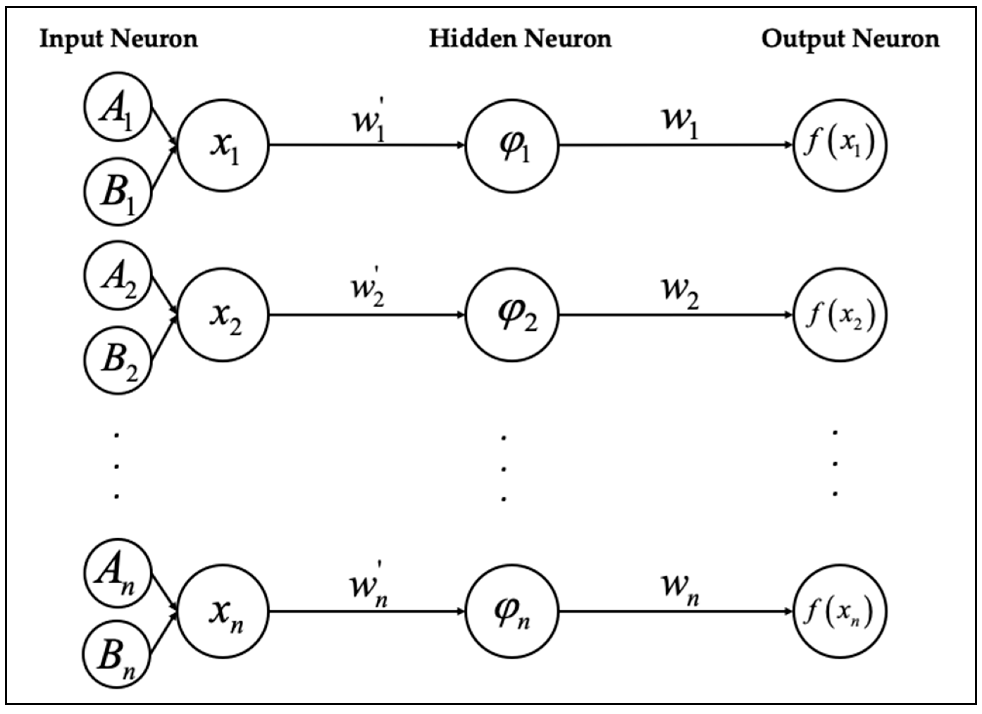
2.2. 2 Satisfiability in Radial Basis Neural Network

Radial Basis Function Neural Network (RBFNN) is a feedforward neural network. Here we consider only three-layers: an input layer, a hidden layer with Radial Basis function as activation units, and the final output layers. The most classical approach in RBFNN is to find the parameters for each layer by using unsupervised learning which leads to suboptimal output weight [34,35]. In this section, systematic input data via $P_{2SAT}$ will be embedded during the training phase of RBFNN. $P_{2SAT}$ will create a systematic partition between input neuron and the output neuron by obtaining a true value of RBFNN as an input data. During training phase of RBFNN, the input data for each clause in $P_{2SAT}$ is given in the following equation:

$$x_i={\displaystyle \sum _{i=1}^{n}I\left(A_i\right)}+{\displaystyle \sum _{j=1}^{n}I\left(B_j\right)}\hspace{0.17em}$$

(3)

where each of the state of the variable in Equation (3) can be defined as follows

$$I\left(A_i\right)\hspace{0.17em}or\hspace{0.17em}I\left(\hspace{0.17em}{B}_j\right)=\{\begin{array}{l}1,\hspace{0.17em}if\hspace{0.17em}A\hspace{0.17em}or\hspace{0.17em}B\hspace{0.17em}is\hspace{0.17em}True\\ 0,\hspace{0.17em}if\hspace{0.17em}A\hspace{0.17em}or\hspace{0.17em}B\hspace{0.17em}is\hspace{0.17em}False\end{array}$$

(4)

Note that, $\left\{0,1\right\}$ indicates the Boolean values that exemplify False and True respectively. Consider the following $P_{2SAT}$ in the form of logic programming:

$$P_{2SAT}=A;B\leftarrow ,\hspace{0.17em}D\leftarrow C,\hspace{0.17em}E\leftarrow F$$

(5)

Note that $\leftarrow$ is a symbol of implication, which is a standard notation in logic programming. ($;$) refers to the ($\vee$), ($,$) is the ($\wedge$). In terms of the variable, ($A;B\leftarrow$) represents $A;B$ as the positives variables and $\leftarrow C$ represent $C$ as negative variable [36]. Converting Equation (5) into Boolean Algebra CNF form

$$P_{2SAT}=\left(A\vee B\right)\wedge \left(\neg C\vee D\right)\wedge \left(E\vee \neg F\right)$$

(6)

where $\neg$ refers to the negation of the variables, $\vee$ is the Disjunction (OR), and $\wedge$ is the Conjunction (AND). According to Equation (6), RBFNN contains 6 variables that will represent the input neurons with 3 clauses which represent output neurons. In this case, the training pattern will be obtained by determining the number of hidden neurons used. The input data of the $P_{2SAT}$ in Equations (5) and (6) is given in

Table 1. The input data form and the training data of $P_{2SAT}$ in Radial Basis Function Neural Network (RBFNN).

Clause	$A;B\leftarrow$	$D\leftarrow C$	$E\leftarrow F$
DNF	$A\vee B$	$\neg C\vee D$	$E\vee \neg F$
Input data form$x_i$	$x=A+B$	$x=D-C$	$x=E-F$
Input data in the training set	0 1 1 2	−1 0 0 1	−1 0 0 1
TheTarget Output data$y_i$	0 1 1 1	0 1 1 1	0 1 1 1

.

From Table 1, the input data $x_i$ will be used to calculate the parameters such as the width, ${\sigma }_i$ and center, $c_i$ in the hidden layer. $y_i$ is the target output that will be used in finding the output weight of RBFNN. Hence, the center of the hidden layer will be calculated by using the following equation:

$$c_i=\frac{1}{m}{\displaystyle \sum _{i=1}^{NH}{x}_i}$$

(7)

where $m$ is the number of literal for each clause in $P_{2SAT}$, and $NH$ is the number of the hidden neuron. The distance $d_i$ between input data and the center of the hidden layer is calculated by using:

$$d_i=\Vert w_i^{\prime }{x}_i-c_i\Vert$$

(8)

In our case, we considered $w_i^{\prime }=1$ as the input weight between input neuron and hidden neuron [37]. By using the distance in Equation (8), the width of each hidden neurons in hidden layer is:

$${\sigma }_i^2=\frac{1}{m}{\displaystyle \sum _{i=1}^{NH}{\left[d\left(x_i,\hspace{0.17em}{c}_i\right)\right]}^{\hspace{0.17em}2}}$$

(9)

Based on the value of the $c_i$ and ${\sigma }_i$, the Gaussian Function of the hidden layer based on $P_{2SAT}$ is

$${\phi }_i\left(x\right)=e^{-\frac{{\Vert {\displaystyle \sum _{i=1}^n{x}_i-c_i}\Vert }^2}{2{\sigma }_i^2}}.$$

(10)

By using $y_i$ and ${\varphi }_i$ the corresponding output weight $w_i$ is calculated implicitly by using:

$$y_i={\displaystyle \sum _{i=1}^n{w}_i{\varphi }_i\left(x_i\right)}$$

(11)

where $y_i$ is the target output obtained from Table 1. Hence, the final output classification of the RBFNN $f\left(x_i\right)$ is expressed as

$$f\left(x_i\right)=\{\begin{array}{l}1,\hspace{0.17em}{\displaystyle \sum _{i=1}^n{w}_i{\varphi }_i\left(x_i\right)\ge 0}\\ 0,\hspace{0.17em}{\displaystyle \sum _{i=1}^n{w}_i{\varphi }_i\left(x_i\right)<0}\end{array}$$

(12)

The proposed RBFNN in this paper is different from Hamadneh et al. [21]. In their article, Horn SAT and general SAT were utilized to calculate the input data. One of the drawback of non-systematic logical rule is the need to approximate the number of hidden neuron in RBFNN. By that standard, the number of hidden neurons for $P_{2SAT}$ is always between the number of input neurons and output neurons. Figure 1 and Figure 2 show the implementation and structure of $P_{2SAT}$ in RBFNN.

2.3. Satisfiability Programming in Hopfield Neural Network

The notion of doing logic programming in ANN is a relatively new concept. The whole concept of logic programming in ANN is to obtain the final neuron state that behaves according to pre-determined systematic logical rule. Since the popularized version of this perspective emerged from doing logic programming in Hopfield Neural Network (HNN), we will examine the structure of HNN as a benchmark of ANN against our proposed network which is RBFNN. HNN is a recurrent neural network [38], consists of interconnected neuron $S_i$ and is divided into input and output layers with no hidden layer involved. The connection between $S_i$ and $S_j$ are given as $S_{ij}$ where both neurons are connected by Synaptic weight, $W_{ij}$. The general definition of the neuron update is given as follows:

$$S_i=\{\begin{array}{l}\hspace{0.17em}1,\hspace{0.17em}if\hspace{0.17em}{\displaystyle \sum _{j=1}^N{W}_{ij}{S}_j}>\xi \\ -1,\hspace{0.17em}otherwise\end{array}$$

(13)

where $\xi$ is a pre-defined threshold. According to Cantini and Caselle [39], the asynchronous neuron update is necessary to ensure the convergence of the network. $P_{2SAT}$ can be implemented in HNN by assigning neuron for each variable. The primary aim of the network is to reduce the logical inconsistencies by minimizing the following cost function:

$$E_{P_{2SAT}}={\displaystyle \sum _{i=1}^{NC}{\displaystyle \prod _{j=1}^{NV}{L}_{ij}}}$$

(14)

where $NC$ and $NV$ are denoted as the number of clauses and variables, respectively. Note that, the inconsistencies of logical clause $L_{ij}$ is given as follows:

$$L_{ij}=\{\begin{array}{l}\frac{1}{2}\left(1-S_x\right),\hspace{0.17em}if\neg x\\ \frac{1}{2}\left(1+S_x\right),\hspace{0.17em}otherwise\end{array}$$

(15)

It is worth mentioning that the synaptic weight of HNN is derived by using Wan Abdullah method [11] whereas $E_{P_{2SAT}}$ is compared with the following final energy function $H_{P_{2SAT}}$

$$H_{P_{2SAT}}=-\frac{1}{2}{\displaystyle \sum _{i=1,\hspace{0.17em}i\ne j}^N{\displaystyle \sum _{j=1,\hspace{0.17em}i\ne j}^N{W}_{ij}^{\left(2\right)}{S}_i{S}_j}-{\displaystyle \sum _{i=1}^N{W}_i^{\left(1\right)}{S}_j}}$$

(16)

For example, by comparing the cost functions defined in Equations (14) and (15) with Equation (16), the synaptic weights that connect the neurons in Equations (5) and (6) are $\left(W_{AB}^{\left(2\right)},W_{CD}^{\left(2\right)},W_{EF}^{\left(2\right)}\right)=\left(-0.25,-0.25,-0.25\right)$, $W_{AA}^{\left(2\right)}=W_{BB}^{\left(2\right)}=W_{CC}^{\left(2\right)}=W_{DD}^{\left(2\right)}=W_{EE}^{\left(2\right)}=W_{FF}^{\left(2\right)}=0$ with no self-connection for second order and $\left(W_A^{\left(1\right)},W_B^{\left(1\right)},W_C^{\left(1\right)},W_D^{\left(1\right)},W_E^{\left(1\right)},W_F^{\left(1\right)}\right)=\left(0.25,0.25,0.25,0.25,0.25,0.25\right)$ for first order. The final state of the neuron can be obtained by computing the local field $h_i\left(t\right)$ of the network:

$$h_i\left(t\right)={\displaystyle \sum _{j=1}^N{W}_{ij}^{\left(2\right)}{S}_j+W_i^{\left(1\right)}}$$

(17)

where the final state of the neuron is given a follows:

$$S_i=\{\begin{array}{l}\hspace{0.17em}1,\hspace{0.17em}if\hspace{0.17em}{\displaystyle \sum _{j=1,i\ne j}^N{W}_{ij}^{\left(2\right)}{S}_j+W_i^{\left(1\right)}}\ge 0\\ -1,\hspace{0.17em}if\hspace{0.17em}{\displaystyle \sum _{j=1,i\ne j}^N{W}_{ij}^{\left(2\right)}{S}_j+W_i^{\left(1\right)}}<0\end{array}$$

(18)

Note that, the value of the global minimum energy, $H_{P_{2SAT}}^{\min }$ can be pre-calculated because the magnitude of the energy for each clause is always constant [30,36]. Hence, the optimized neuron state can be obtained by examining $\left|H_{P_{2SAT}}^{\min }-H_{P_{2SAT}}\right|\le \partial$ where $\partial$ is pre-defined by the user.

3. Experimental Setup

In this paper, the proposed network (RBFNN) and the existing network (HNN) were executed by using Microsoft Visual#2008 Express software as a platform for simulation. Then, the simulations were carried out by using the same processor, with the specification: 3.40 GHz processor, 4096 MB RAM via Windows 10.1 operating system. In order to attain fair comparison, the models were terminated after being executed for no more than 24 h. Simulated data is a randomly generated data by our program during the simulation. In this case, the simulated dataset will be obtained by generating random clauses and literals for a particular $P_{2SAT}$. The generated data considers the binary values with the structure based on the number of clauses defined by the researchers. Thus, the simulated data is commonly used to authenticate the performance of our proposed networks in discriminating the neuron state, whether it is an optimal or suboptimal neuron state. The concept of simulated data in SAT logic with ANN has been initially coined in the work of Sathasivam and Abdullah [40] and Hamadneh et al. [21]. The learning methods for HNN and RBFNN are based on the Genetic Algorithm proposed in Kasihmuddin et al. [27] for HNN and Hamadneh et al. [22] for RBFNN. Based on the simulations for HNN and RBFNN, the quality of the retrieval phase of $P_{2SAT}$ are assessed by using numerous performance metrics, such as, Root Mean Square Error (RMSE), Sum of Squared Error (SSE), Mean Absolute Percentage Error (MAPE) and Central Processing Unit (CPU) time. The formula that calculate each error are given as follows:

$$RMSE={\displaystyle \sum _{i=1}^n\sqrt{\frac{1}{n}{\left(f\left(x_i\right)-y_i\right)}^2}}$$

(19)

$$SSE={\displaystyle \sum _{i=1}^n{\left(f\left(x_i\right)-y_i\right)}^2}$$

(20)

$$MAPE=\frac{100}{n}{\displaystyle \sum _{i=1}^n\left|\frac{f\left(x_i\right)-y_i}{y_i}\right|}$$

(21)

where $f\left(x_i\right)$ is the output value, $y_i$ is the target output value, and $n$ is number of the iterations. RMSE is a measure of error deviation around the average for non-Satisfiable neurons. In this case, this metric examines the distribution of the error around the Satisfiable neuron state. The accumulation of error can be examined by using SSE. SSE is very sensitive to small error and magnifies each wrong final state and makes it empirically validated. In addition, the fraction of the non-Satisfiable neuron state can be measured by the use of MAPE. In this case, the higher MAPE value suggests the higher proportion of the suboptimal neuron state.

It is worth mentioning that the final output for HNN will be converted to binary representation before we evaluate the performance error by using Equations (19)–(21). In addition, both networks with a different initial neuron state will lead to the biasedness of the retrieval state due to the fact that the network simply overfits with the computational environment. Thus, the network will transform into a phase whereby it memorizes the final state without producing a brand new state. In order to avoid such circumstances, all possible positive and negative bias can be minimized by producing all the neuron states randomly. The randomization scheme for HNN and RBFNN are shown in Equations (22) and (23)

$$\left(S_1^{HNN},S_2^{HNN},S_3^{HNN},\dots ,S_N^{HNN}\right)=\{\begin{array}{l}\hspace{0.17em}1,\hspace{0.17em}rand\left(0,1\right)<0.5\\ -1,\hspace{0.17em}otherwise\end{array}$$

(22)

where the states of true and false are given as 1 and −1, respectively.

$$\left(S_1^{RBFNN},S_2^{RBFNN},S_3^{RBFNN},\dots ,S_N^{RBFNN}\right)=\{\begin{array}{l}1,\hspace{0.17em}rand\left(0,1\right)<0.5\\ 0,\hspace{0.17em}otherwise\end{array}$$

(23)

where the states of true and false are given as 1 and 0, respectively. Note that, the number of neuron combination used in HNN is set to be 100, with energy tolerance being set to $\partial =0.001$ and number of learning cycle $\Omega =100$ [12,27]. Subsequently, the parameters for the both RBFNN model are summarized systematically in

Table 2. List of Parameters in RNFNN.

Parameter	Parameter Value
Neuron Combination	100
Tolerance Value $(\partial )$	0.001
Number of Learning Cycle $(\Omega )$	100
No_Neuron String	100
Input data $\left(x_i\right)$	$x_i\in \left\{-1,0,1,2\right\}$
No_Chromosomes	100
Generation	1000
Selection_Rate	0.1
Mutation_Rate	0.01
Crossover_Rate	0.9

.

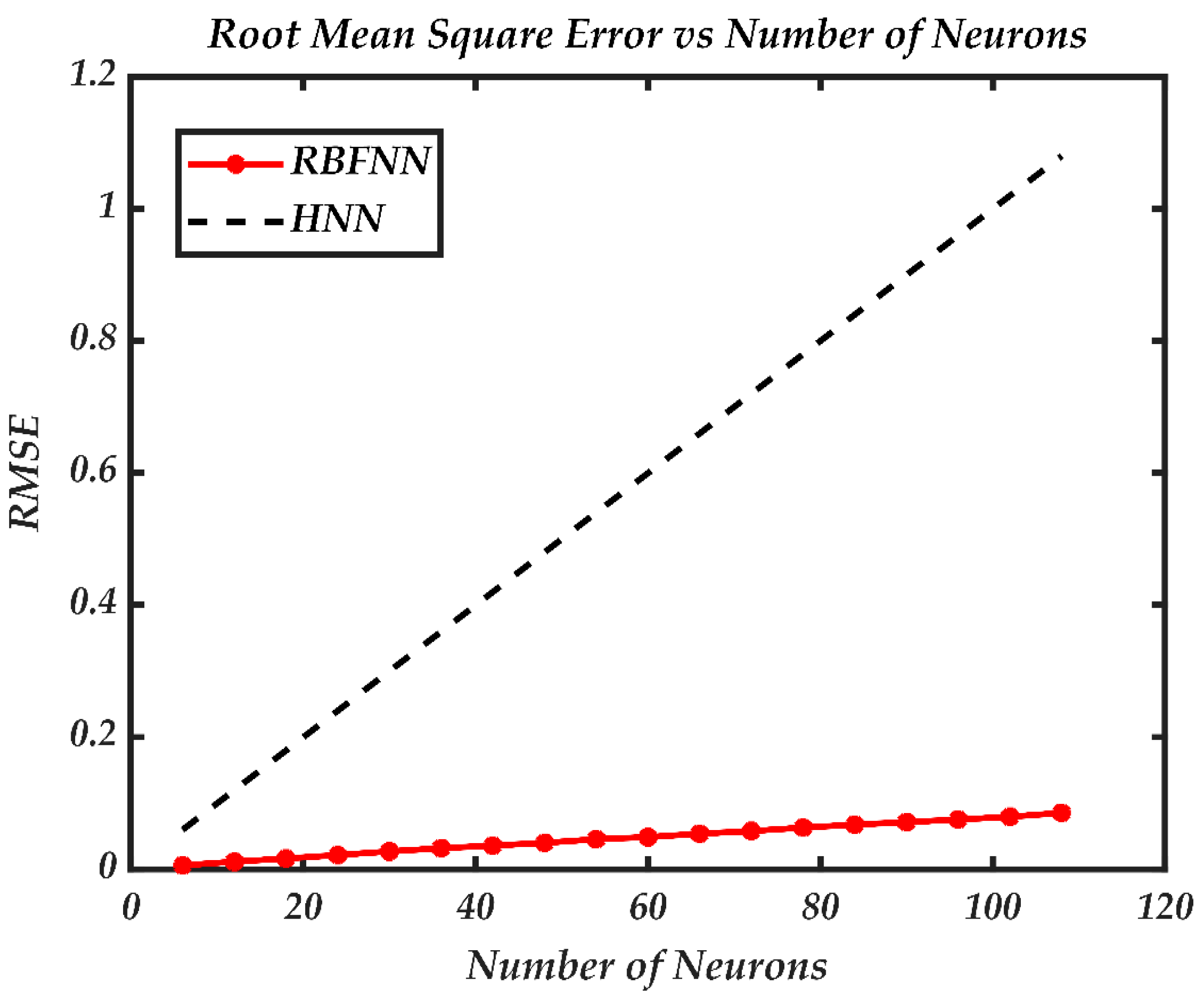
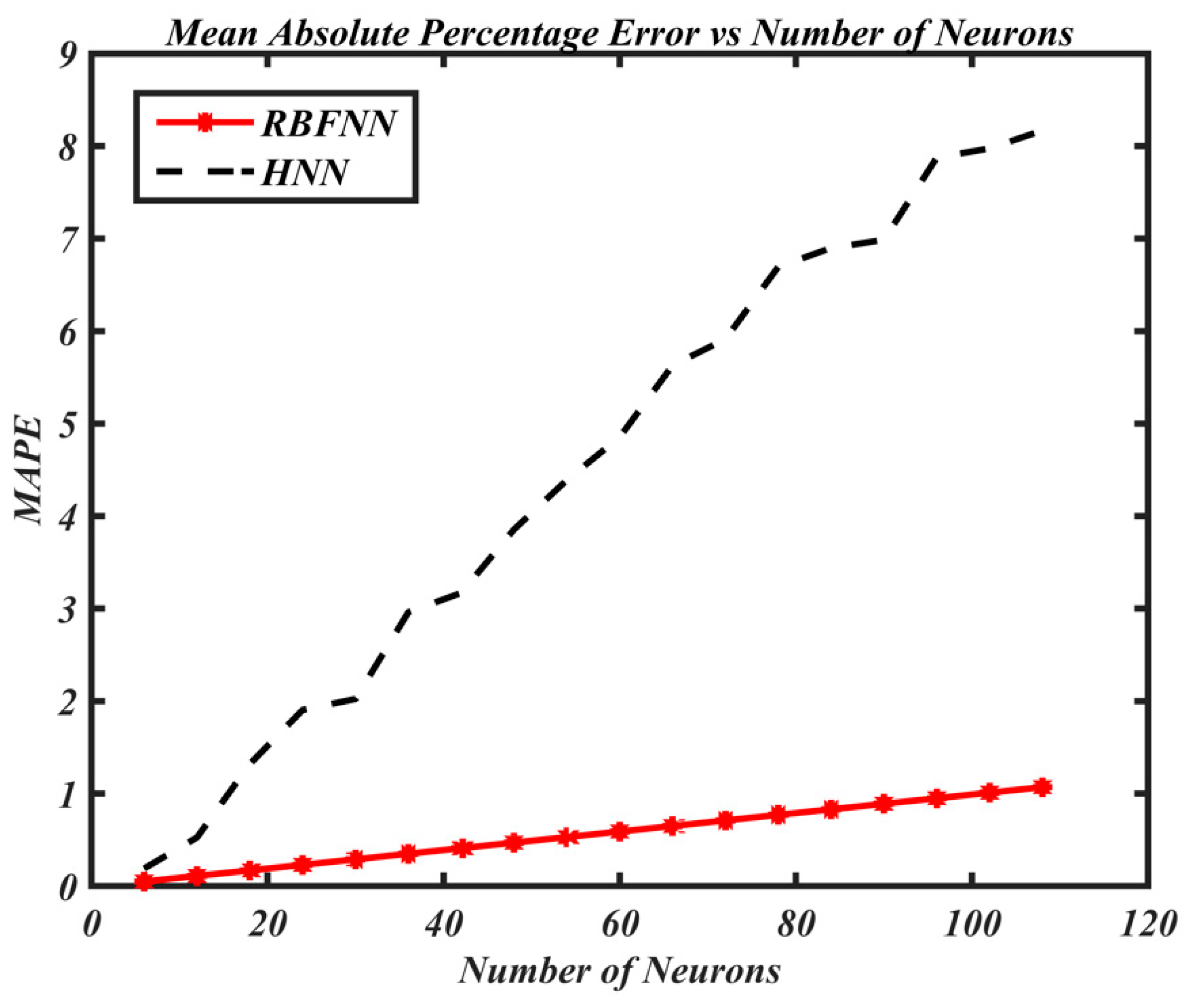
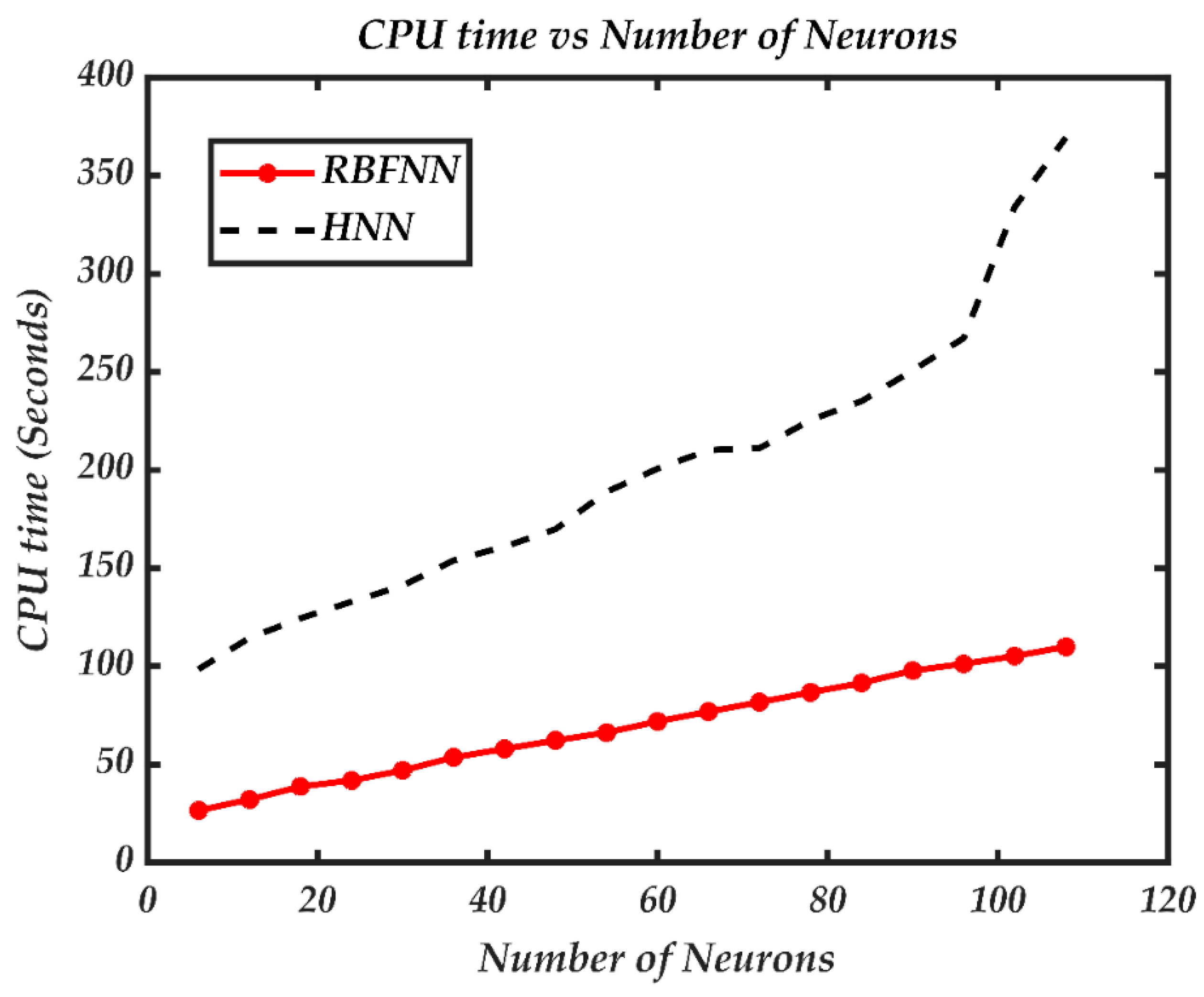
4. Result and Discussion

In this section, the evaluation results for both proposed models of RBFNN and HNN are presented based on $P_{2SAT}$. Both systems are evaluated based on the RMSE, SSE, MAPE and CPU time.

Figure 3 and Figure 4 show the RMSE and SSE for the proposed model RBFNN and existing approach, HNN from $NN=6$ to $NN=108$, in $P_{2SAT}$. According to Figure 3, RBFNN has the lowest value of RMSE for all the number of neurons as compared to HNN. Specifically, during $NN=60$, RBFNN recorded 91.78% lower than HNN in terms of RMSE. $P_{2SAT}$ is observed to comply with RBFNN which a feed-forward neural network in obtaining the optimal weight. Based on Figure 3, it can be seen that the value of RMSE recorded by HNN was increasing significantly from $NN=6$ until $NN=108$. The higher value of RMSE manifests the lower performance of HNN in generating the optimal final state for $P_{2SAT}$. Figure 4 depicts the value of SSE obtained by RBFNN and HNN for a different number of the neuron. The value of SSE recorded in RBFNN is apparently lower than in HNN, indicating that the RBFNN has a significant effect in obtaining the optimal final state for $P_{2SAT}$ logical rule. According to the value of MAPE in Figure 5, it was obvious that our proposed RBFNN recorded MAPE consistently less than 1% for all number of neurons. On the contrary, the MAPE for HNN increases significantly up to 8% until the last simulations. The fraction of non-Satisfiable neuron for HNN can be seen as significantly higher than RBFNN. The lower value of fraction of non-Satisfiable neuron provides profound evidence of the performance of RBFNN to work well with $P_{2SAT}$ programming. The optimization operators during obtaining the output weight and final outputs have minimized the percentage of suboptimal state as opposed to HNN.

Figure 6 shows the CPU time for the proposed model, RBFNN and existing approach, HNN in $P_{2SAT}$ programming. CPU time is defined as the execution time taken by the model to generate the final neuron state. Generally, as the number of the neuron increase, we can observe that the CPU time will increase over the number of the neurons. The plot of the CPU time in Figure 6 revealed that the compatibility and capability of RBFNN in generating the final neuron state with different complexity in terms of the different numbers of the neuron. It can be seen clearly that the execution time RBFNN is faster than HNN, indicating that RBFNN has outperformed HNN in terms of the robustness of the network. The lower value of CPU time indicates the better performance of the proposed model in attaining the convergence (optimal state). Specifically, when the $NN=90$, the RBFNN executes the program 60.99% faster than HNN. Therefore, the obvious difference in the CPU time can be observed ominously from $NN=6$ until $NN=108$. The above results show that the RBFNN outperformed HNN in generating the optimal state $P_{2SAT}$ with different complexity. Apart from indicating the robustness and computational speed, CPU time also describes the complexity of the networks in this research. The complexity of RBFNN and HNN can described as linear as suggested from the CPU time recorded in Figure 5. Both models proven to deal with higher-order neurons, even though the computational burden is getting higher.

The simulation also provides evidence that RBFNN can obtain the optimized weight by optimally connecting the hidden layer and output layer. The loss of information from the input layer is minimized due to the Gaussian Function and the optimized parameters. Hence, the optimized weight reduced the possible neuron oscillation during training. We estimate that the performance of RBFNN will be similar if the simulation is repeated with another systematic logical rule proposed in Dahllöf et al. [41]. On the other hand, HNN has been proven by Hopfield [42] to converge to the nearest local minimum energy. This is an interesting result considering the result in RBFNN agrees with the trend by outperforming the error illustrated by HNN. This comparison is considered significant because this simulation compares both the ANN structure with different discipline (Recurrent and Feedforward ANN). $P_{2SAT}$ reduces the computational burden by fixing the number of hidden neurons in the hidden layer in RBFNN. The constant value of the hidden neurons in the hidden layer reduces the possible error during the retrieval phase. The limitation of the proposed RBFNN is the network only considers Satisfiable formula. Another non-Satisfiable logical rule such as Maximum Satisfiability [43] and Minimum Satisfiability [44] requires more specified neuron partition to reduce complexity in the hidden layer. Different logical rules must be investigated in depth to verify the effectiveness of the systematic logical rule in RBFNN. Besides, other latest metaheuristics such as Artificial Bee Colony [45] and Grey Wolf Optimization algorithm [46] are required to reduce heavy computation during the training phase. Furthermore, our proposed RBFNN is not guaranteed to perform optimally in another set of NP problems. This observation is in accordance with No Free Lunch Theorem [47] where the proposed method is not universally superior for all type of problems. The Satisfiability formula can be used to generalize and extract the information from the data set of various applications. Thus, we believe that our proposed RBFNN integrated with $P_{2SAT}$ has the potential to be an alternative for the standard RBFNN in processing numerous types of data ranging from the medical classification, industrial automation and stock market prediction. The existing RBFNN can be integrated with a systematic logical rule such as $P_{2SAT}$ and reduce the computational burden for the parameters.

5. Conclusions

We have shown the capability of $P_{2SAT}$ in optimizing the final state obtained by the RBFNN. We have also shown that the embedded systematic $P_{2SAT}$ in RBFNN has reduced the computational burden significantly for all of RBFNN parameters. This result has manifested a massive leap in the development of RBFNN itself, especially in terms of producing the best weight to connect the input and output layer effectively with minimum errors. Hence, the impact of optimized output weights generated by RBFNN has successfully enhanced the training with different levels of complexities. The stability of the $P_{2SAT}$ logical rule in RBFNN can be attained due to the fewer number of the neuron in the hidden layer than other rules. Based on this research, we can conclude the conventional learning method [11,12] is not necessarily ideal in output weight optimization in ANN. Our proposed model, RBFNN has outperformed the HNN in the compatibility with the $P_{2SAT}$. On all cases and complexities, the $P_{2SAT}$ logical rule has proven to optimize the parameters for RBFNN, which is a feed-forward neural network. Using this approach, the error and robustness measures are well presented, indicating the performance of $P_{2SAT}$ optimized RBFNN model.

The evolution of the systematic $P_{2SAT}$ logical rule optimization is still in the infancy stage and requires more in-depth research especially in the other variant of the neural network, especially feed-forward neural network. In the future, we will venture the deep convolutional neural network [48] and optimize the possible parameters via $P_{2SAT}$. Our research can be further employed by manipulating different variant of logical rule such as randomized k Satisfiability (Rand kSAT) [49] and other Unsatisfiable logical rule, namely Weighted Maximum Satisfiability (Weighted MAX-SAT) [50] and Minimum Satisfiability (MIN-SAT) [51]. We would be able to extend the structure of optimized $P_{2SAT}$ with RBFNN as the knowledge extraction paradigm via logic mining perspective. In fact, the direction will open numerous opportunities for real life applications. Additionally, the RBFNN parameters can be optimized by integrating robust Metaheuristic algorithms such as Ant Lion Optimization approach [52], Harmony Search [53], modified Flower Pollination Algorithm [54], fine-tuning Metaheuristics [55] and particle swarm optimization algorithm [56].

References

1. Moody, J.; Darken, C.J. Fast learning in networks of locally-tuned processing units. Neural Comput. 1989, 1, 281–294. [Google Scholar] [CrossRef]
2. Celikoglu, H.B. Application of radial basis function and generalized regression neural networks in non-linear utility function specification for travel mode choice modelling. Math. Comput. Model. 2006, 44, 640–658. [Google Scholar] [CrossRef]
3. Guo, Z.; Wang, H.; Yang, J.; Miller, D.J. A stock market forecasting model combining two-directional two-dimensional principal component analysis and radial basis function neural network. PLoS ONE 2015, 10, e0122385. [Google Scholar] [CrossRef] [PubMed] [Green Version]
4. Roshani, G.H.; Nazemi, E.; Roshani, M.M. Intelligent recognition of gas-oil-water three-phase flow regime and determination of volume fraction using radial basis function. Flow Meas. Instrum. 2017, 54, 39–45. [Google Scholar] [CrossRef]
5. Hjouji, A.; El-Mekkaoui, J.; Jourhmane, M.; Qjidaa, H.; Bouikhalene, B. Image retrieval and classication using shifted legendre invariant moments and radial basis functions neural networks. Procedia Comput. Sci. 2019, 148, 154–163. [Google Scholar] [CrossRef]
6. Dash, C.S.K.; Behera, A.K.; Dehuri, S.; Cho, S.B. Building a novel classifier based on teaching learning based optimization and radial basis function neural networks for non-imputed database with irrelevant features. Appl. Comput. Inform. 2019. [Google Scholar] [CrossRef]
7. Park, J.; Sandberg, I.W. Universal approximation using radial-basis-function networks. Neural Comput. 1991, 3, 246–257. [Google Scholar] [CrossRef]
8. Sing, J.K.; Basu, D.K.; Nasipuri, M.; Kundu, M. Improved k-means algorithm in the design of RBF neural networks. In Proceedings of the TENCON 2003 Conference on Convergent Technologies for Asia-Pacific Region, Bangalore, India, 15–17 October 2003; pp. 841–845. [Google Scholar]
9. Gholami, A.; Bonakdari, H.; Zaji, A.H.; Fenjan, S.A.; Akhtari, A.A. New radial basis function network method based on decision trees to predict flow variables in a curved channel. Neural Comput. Appl. 2018, 30, 2771–2785. [Google Scholar] [CrossRef]
10. Jafrasteh, B.; Fathianpour, N. A hybrid simultaneous perturbation artificial bee colony and back-propagation algorithm for training a local linear radial basis neural network on ore grade estimation. Neurocomputing 2017, 235, 217–227. [Google Scholar] [CrossRef]
11. Abdullah, W.A.T.W. Logic programming on a neural network. Int. J. Intell. Syst. 1992, 7, 513–519. [Google Scholar] [CrossRef]
12. Sathasivam, S. Upgrading logic programming in Hopfield network. Sains Malays. 2010, 39, 115–118. [Google Scholar]
13. Yang, J.; Wang, L.; Wang, Y.; Gou, T. A novel memristive Hopfield neural network with application in associative memory. Neurocomputing 2017, 227, 142–148. [Google Scholar] [CrossRef]
14. Sathasivam, S. Learning rules comparison in Neuro-Symbolic integration. Int. J. Appl. Phys. Math. 2011, 1, 129–132. [Google Scholar] [CrossRef] [Green Version]
15. Yang, G.; Wu, S.; Jin, Q.; Xu, J. A hybrid approach based on stochastic competitive Hopfield neural network and efficient genetic algorithm for frequency assignment problem. Appl. Soft Comput. 2016, 39, 104–116. [Google Scholar] [CrossRef]
16. Mansor, M.A.; Kasihmuddin, M.S.M.; Sathasivam, S. Enhanced Hopfield network for pattern satisfiability optimization. Int. J. Intell. Syst. Appl. 2016, 8, 27. [Google Scholar] [CrossRef]
17. Sathasivam, S.; Pei, F.N. Developing agent based modeling for doing logic programming in hopfield network. Appl. Math. Sci. 2013, 7, 23–35. [Google Scholar]
18. Mansor, M.A.; Kasihmuddin, M.S.M.; Sathasivam, S. VLSI circuit configuration using satisfiability logic in Hopfield network. Int. J. Intell. Syst. Appl. 2016, 8, 22–29. [Google Scholar] [CrossRef]
19. Sathasivam, S.; Abdullah, W.A.T.W. Logic mining in neural network: Reverse analysis method. Computing 2011, 91, 119–133. [Google Scholar] [CrossRef]
20. Sathasivam, S.; Hamadneh, N.; Choon, O.H. Comparing neural networks: Hopfield network and RBF network. Appl. Math. Sci. 2011, 5, 3439–3452. [Google Scholar]
21. Hamadneh, N.; Sathasivam, S.; Choon, O.H. Higher order logic programming in radial basis function neural network. Appl. Math. Sci. 2012, 6, 115–127. [Google Scholar]
22. Hamadneh, N.; Sathasivam, S.; Tilahun, S.L.; Choon, O.H. Learning logic programming in radial basis function network via genetic algorithm. J. Appl. Sci. 2012, 12, 840–847. [Google Scholar] [CrossRef]
23. Glaßer, C.; Jonsson, P.; Martin, B. Circuit satisfiability and constraint satisfaction around Skolem Arithmetic. Theor. Comput. Sci. 2017, 703, 18–36. [Google Scholar] [CrossRef]
24. Jensen, L.S.; Kaufmann, I.; Larsen, K.G.; Nielsen, S.M.; Srba, J. Model checking and synthesis for branching multi-weighted logics. J. Log. Algebraic Methods Program. 2019, 105, 28–46. [Google Scholar] [CrossRef]
25. Pearce, B.; Kurz, M.E.; Phelan, K.; Summers, J.; Schulte, J.; Dieminger, W.; Funk, K. Configuration management through satisfiability. Procedia CIRP 2016, 44, 204–209. [Google Scholar] [CrossRef] [Green Version]
26. Mansor, M.A.; Sathasivam, S. Accelerating activation function for 3-satisfiability logic programming. Int. J. Intell. Syst. Appl. 2016, 8, 44. [Google Scholar] [CrossRef] [Green Version]
27. Kasihmuddin, M.S.M.; Mansor, M.A.; Sathasivam, S. Hybrid genetic algorithm in the Hopfield network for logic satisfiability problem. Pertanika J. Sci. Technol. 2017, 25, 139. [Google Scholar]
28. Kasihmuddin, M.S.M.; Mansor, M.A.; Sathasivam, S. Satisfiability based reverse analysis method in diabetes detection. In Proceedings of the 25th National Symposium on Mathematical Sciences (SKSM25), Pahang, Malaysia, 27–29 August 2017; p. 020020. [Google Scholar]
29. Kasihmuddin, M.S.M.; Mansor, M.; Sathasivam, S. Robust artificial bee colony in the Hopfield network for 2-satisfiability problem. Pertanika J. Sci. Technol. 2017, 25, 453–468. [Google Scholar]
30. Kasihmuddin, M.S.M.; Mansor, M.A.; Basir, M.F.M.; Sathasivam, S. Discrete Mutation Hopfield Neural Network in Propositional Satisfiability. Mathematics 2019, 7, 1133. [Google Scholar] [CrossRef] [Green Version]
31. Gramm, J.; Hirsch, E.A.; Niedermeier, R.; Rossmanith, P. Worst-case upper bounds for max-2-sat with an application to max-cut. Discret. Appl. Math. 2003, 130, 139–155. [Google Scholar] [CrossRef] [Green Version]
32. Avis, D.; Tiwary, H.R. Compact linear programs for 2SAT. Eur. J. Comb. 2019, 80, 17–22. [Google Scholar] [CrossRef] [Green Version]
33. Fürer, M.; Kasiviswanathan, S.P. Algorithms for counting 2-SAT solutions and colorings with applications. In Proceedings of the International Conference on Algorithmic Applications in Management, Portland, OR, USA, 6–8 June 2007; pp. 47–57. [Google Scholar]
34. Sheta, A.F.; De Jong, K. Time-series forecasting using GA-tuned radial basis functions. Inf. Sci. 2001, 133, 221–228. [Google Scholar] [CrossRef]
35. Chaiyaratana, N.; Zalzala, A.M.S. Evolving hybrid RBF-MLP networks using combined genetic/unsupervised/supervised learning. In Proceedings of the UKACC International Conference on Control (CONTROL ’98), Swansea, UK, 1–4 September 1998; pp. 330–335. [Google Scholar]
36. Sathasivam, S. Improving Logic Programming in Hopfield Network with Sign Constrained. In Proceedings of the International Conference on Computer Technology and Development, Kota Kinabalu, Malaysia, 13–15 November 2009; pp. 161–164. [Google Scholar]
37. Hamadneh, N.; Sathasivam, S.; Choon, O.H. Computing single step operators of logic programming in radial basis function neural networks. In Proceedings of the 21st National Symposium on Mathematical Sciences (SKSM21), Penang, Malaysia, 6–8 August 2013; pp. 458–463. [Google Scholar]
38. Hopfield, J.J.; Tank, D.W. “Neural” computation of decisions in optimization problems. Biol. Cybern. 1985, 52, 141–152. [Google Scholar] [PubMed]
39. Cantini, L.; Caselle, M. Hope4Genes: A Hopfield-like class prediction algorithm for transcriptomic data. Sci. Rep. 2019, 9, 1–9. [Google Scholar] [CrossRef] [PubMed] [Green Version]
40. Sathasivam, S.; Wan Abdullah, W.A.T. Logic learning in Hopfield Networks. Mod. Appl. Sci. 2008, 2, 57–63. [Google Scholar] [CrossRef]
41. Dahllöf, V.; Jonsson, P.; Wahlström, M. Counting models for 2SAT and 3SAT formulae. Theor. Comput. Sci. 2005, 332, 265–291. [Google Scholar] [CrossRef] [Green Version]
42. Hopfield, J.J. Neuron with graded response have computational properties like those of two-state neurons. Proc. Natl. Acad. Sci. USA 1984, 81, 3088–3092. [Google Scholar] [CrossRef] [Green Version]
43. Paul, A.; Poloczek, M.; Williamson, D.P. Simple approximation algorithms for balanced MAX 2SAT. Algorithmica 2018, 80, 995–1012. [Google Scholar] [CrossRef]
44. Li, C.M.; Zhu, Z.; Manyà, F.; Simon, L. Optimizing with minimum satisfiability. Artif. Intell. 2012, 190, 32–44. [Google Scholar] [CrossRef]
45. Karaboga, D.; Basturk, B. Artificial Bee Colony (ABC) optimization algorithm for solving constrained optimization problems. In Proceedings of the 12th International Fuzzy Systems Association World Congress (IFSA 2007), Cancun, Mexico, 18–21 June 2007; pp. 789–798. [Google Scholar]
46. Emary, E.; Zawbaa, H.M.; Hassanien, A.E. Binary grey wolf optimization approaches for feature selection. Neurocomputing 2016, 172, 371–381. [Google Scholar] [CrossRef]
47. Koppen, M.; Wolpert, D.H.; Macready, W.G. Remarks on a recent paper on the “no free lunch”. IEEE Trans. Evolut. Comput. 2001, 5, 295–296. [Google Scholar] [CrossRef]
48. Poria, S.; Cambria, E.; Gelbukh, A. Aspect extraction for opinion mining with a deep convolutional neural network. Knowl. Based Syst. 2016, 108, 42–49. [Google Scholar] [CrossRef]
49. Ricci-Tersenghi, F.; Weigt, M.; Zecchina, R. Simplest random k-satisfiability problem. Phys. Rev. E 2001, 63, 026702. [Google Scholar] [CrossRef] [PubMed] [Green Version]
50. Xing, Z.; Zhang, W. MaxSolver: An efficient exact algorithm for (weighted) maximum satisfiability. Artif. Intell. 2005, 164, 47–80. [Google Scholar] [CrossRef] [Green Version]
51. Kohli, R.; Krishnamurti, R.; Mirchandani, P. The minimum satisfiability problem. SIAM J. Discret. Math. 1994, 7, 275–283. [Google Scholar] [CrossRef]
52. Mikaeil, R.; Ozcelik, Y.; Ataei, M.; Shaffiee, H.S. Application of harmony search algorithm to evaluate performance of diamond wire saw. J. Min. Environ. 2019, 10, 27–36. [Google Scholar]
53. Mishra, M.; Barman, S.K.; Maity, D.; Maiti, D.K. Ant lion optimisation algorithm for structural damage detection using vibration data. J. Civ. Struct. Health Monit. 2019, 9, 117–136. [Google Scholar] [CrossRef]
54. Nabil, E. A modified flower pollination algorithm for global optimization. Expert Syst. Appl. 2016, 57, 192–203. [Google Scholar] [CrossRef]
55. Allawi, Z.T.; Ibraheem, I.K.; Humaidi, A.J. Fine-tuning meta-heuristic algorithm for global optimization. Processes 2019, 7, 657. [Google Scholar] [CrossRef] [Green Version]
56. Zhao, Y.; Liao, C.; Qin, Z.; Yang, K. Using PSO algorithm to compensate power loss due to the aeroelastic effect of the wind turbine blade. Processes 2019, 7, 633. [Google Scholar] [CrossRef] [Green Version]
Figure 1. The implementation of P 2 S A T in RBFNN.
Processes 08 00214 g001
Figure 2. Structure of P 2 S A T in RBFNN.
Processes 08 00214 g002
Figure 3. The performance of proposed RBFNN and Hopfield Neural Network (HNN) in term of Root Mean Square Error (RMSE).
Processes 08 00214 g003
Figure 4. The performance of proposed RBFNN and HNN in term of Sum of Squared Error (SSE).
Processes 08 00214 g004
Figure 5. The performance of proposed RBFNN and HNN in term of Mean Absolute Percentage Error (MAPE).
Processes 08 00214 g005
Figure 6. The performance of proposed RBFNN and HNN in term of CPU time.
Processes 08 00214 g006