Investigation of an Improved Polymer Flooding Scheme by Compositionally-Tuned Slugs

Abstract

Polymer flooding is an effective enhanced oil recovery technology used to reduce the mobility ratio and improve sweep efficiency. A new polymer injection scheme is investigated that relies on the cyclical injection of low-salinity, low-concentration polymer slugs chased by high-salinity, high-concentration polymer slugs. The effectiveness of the process is a function of several reservoir and design parameters related to polymer type, concentration, salinity, and reservoir heterogeneity. We use reservoir simulations and design-of-experiments (DoE) to investigate the effectiveness of the proposed polymer injection scheme. We show how key objective functions, such as recovery factor and injectivity, are impacted by the reservoir and design parameters. In this study, simulations showed that the new slug-based process was always superior to the reference polymer injection scheme using the traditional continuous injection scheme. Our results show that the process is most effective when the polymer weight is high, corresponding to large inaccessible pore-volumes, which enhances polymer acceleration. High vertical heterogeneity typically reduces the process performance because of increased mixing in the reservoir. The significance of this process is that it allows for increased polymer solution viscosity in the reservoir without increasing the total mass of polymer, and without impairing polymer injectivity at the well.

1. Introduction

Polymer flooding has been broadly deployed in the industry and is the most commonly used chemical Enhanced Oil Recovery (EOR) method in conventional oilfields [1]. Polymer is typically added to the injected water to increase its viscosity, creating more favorable conditions for oil sweep. Poor sweep efficiency is one of the most challenging problems often encountered during secondary recovery. Poor sweep efficiency arises owing to pronounced reservoir heterogeneity (e.g., the presence of thief layers) and an unfavorable mobility ratio ($M$), where $M$ is defined as:

$$M=\frac{k_{rw}{\mu }_o}{k_{ro}{\mu }_w}$$

(1)

In the above equation, $k_{rw}$, ${\mu }_w$, $k_{ro}$, and ${\mu }_o$ are the relative permeability and viscosity of the water phase and the oil phase, respectively. A displacement is termed unfavorable when $M$ becomes significantly larger than one. Polymer flooding is an enhanced oil recovery technique that improves sweep efficiency by adding polymer molecules to the injected water, which increases the water viscosity, and hence, a reduction of $M$ [1]. A polymer flooding project typically becomes economically viable when the mobility ratio can be reduced by one order of magnitude while the rate of polymer injection (i.e., polymer injectivity) is kept sufficiently high. However, the polymer injectivity degrades with increasing polymer viscosity. Therefore, the successful design of a polymer flooding project requires optimization of a multi-objective problem under uncertainty [2].

1.1. Background

The traditional approach to polymer flooding consists of designing a constant composition of polymer and brine such that the polymer viscosity is maximized while the injectivity is kept high enough to improve project economics. Predicting optimum polymer injectivity is often challenging. If polymer viscosity is set too high, the subsurface formation near the wellbore may experience damage owing to the plugging of pores, and consequently, polymer injectivity may degrade. Recently, Torrealba and Hoteit [3] proposed an alternative injection scheme based on the design of compositionally-tuned slugs. They showed that the EOR scheme could be designed to take advantage of polymer acceleration relative to salt in the reservoir, which often occurs as a result of the discrepancy in the rock pore volumes accessible to polymer and salt components. The proposed process can recover additional oil compared to the traditional approach, without significantly impacting polymer injectivity and without increasing the overall usage of the polymer mass.

The performance of enhanced oil recovery techniques depends on multiple parameters, including the properties of the reservoir rock, the displaced and injected fluid properties, the reservoir rock-fluid interactions, and the extraction method. The parameters related to the rock and the displaced fluid are mostly considered uncontrollable variables, and those related to the injected fluid and the wells are considered controllable or design variables that can be optimized based on the subsurface uncertainties.

To understand the sensitivities of the governing parameters, classical laboratory experiments, or numerical experiments are typically conducted. The former provides reliable observations at a high cost of time and resources. In contrast, the latter provides an efficient alternative to understand the response relative to different objective functions (e.g., oil recovery factor, fluid injectivity) under uncertainty [4,5]. In addition to understanding the recovery behavior, these numerical experiments can be used to define proxy models that allow for the quantitative estimation of the output performance as a function of both uncontrollable and controllable variables. Finally, the numerical experiments can be used to test and confirm the predictability of the proxy models.

A typical approach for designing experiments is to keep all variables constant while modifying only One-Variable-At-a-Time (OVAT). This approach is inefficient, and its success is mostly a function of guesswork, luck, prior experience, and instinct [6]. Further, this approach demands considerable resources and yields limited insights into the process under investigation. Design of Experiments (DoE) was first developed by Fisher [7] to optimize the process of determining the response of different plots of lands as a function of various fertilizers. Fisher [8] formalized this statistical methodology by considering how measures of accuracy and efficiency varied as a function of the number of experiments. Moving forward some 50 years, Sawyer et al. [9] were among the first researchers to use the DoE framework in petroleum engineering to understand the performance of the wet-combustion drive process. Regardless of the industry or application, the ethos of DoE does not change: obtaining maximum information at minimum cost [10,11].

DoE has been extensively used for assessing parameter sensitivity, quantifying uncertainty, and performing optimization in various EOR applications. Ghaderi et al. [12] deployed a D-Optimal design to perform sensitivity analysis and optimization for CO₂-WAG injection. Ogunbanwo and Kovscek [13] utilized a three-level design to explore multiple-parameter interactions in in-situ combustion. Bevillon and Mohagerani [14] used Latin Hypercube design to check sensitivities and quantify uncertainties in a miscible EOR project in the Middle East. Bengar et al. [15] conducted sensitivity analysis for polymer injection using two-level full factorial design. Adepoju et al. [16] proposed a lumped approach to account for parameter dependency in a surfactant-polymer flood and demonstrated their method on a field case. A recent study by Santoso et al. [17] introduced a comprehensive DoE workflow to perform a sensitivity analysis and uncertainty quantification and optimization sequentially. The workflow emphasizes on the use of a two-level design for sensitivity analysis and space-filled augmented design for accurate surrogate modeling. Then, uncertainty quantification or optimization is conducted on the surrogate model. We adopt this workflow to properly assess the interaction of multiple parameters in compositionally-tuned polymer slug injection. Simulations were conducted using the UTChem simulator, developed by the University of Texas at Austin, with DOE support available in its early releases. The simulator is based on the traditional cell-centered finite-difference discretization with IMPES-based (implicit pressure Explicit Saturation) temporal schemes [18,19,20]. It supports various applications including black-oil, multi-component, four-phase for chemical EOR including surfactants and polymers. The code also supports other applications such as groundwater fluid flow and transport, and others. For a complete description of the code, we refer to the user manual [21].

1.2. Factors That Impact Performance in Polymer Flooding

In this section, we review some of the key mechanisms that govern the transport of polymer solutions through porous media, which will allow us to identify the most relevant factors impacting polymer injectivity of oil recovery factor during polymer-based enhanced oil recovery.

Polymer molecular weight ($MW$) is a crucial design parameter in polymer flooding that controls both polymer bulk solution properties as well as polymer-rock interaction. Liauh et al. [22] showed unequivocally that polymer inaccessible pore volume ($IPV$) increases with increasing $MW$. A simplistic interpretation of $IPV$ is that it only depends on the relation of the pore size distribution to the polymer molecular size (i.e., size exclusion). Other considerations are described in recent work by Torrealba and Hoteit [23]. Typical values of $IPV$ for consolidated rock samples range from 7 to 40% [24,25,26,27]. De Gennes [28,29] developed the scaling concept that showed how polymer solution viscosity increases with both $MW$ and polymer concentration. An increase in both salt content and the shear rate has a degrading impact on polymer solution viscosity [30,31,32,33,34].

Polymer adsorption to rocks is determined by the interplay between polymer-surface energy and polymer entropic effects [35]. These factors generally counteract each other, making polymer adsorption one of the most challenging polymer-rock interaction properties to estimate. Large negative polymer-surface energy is considered favorable and leads to higher adsorption. When permeability is low, the ratio of pore-wall surface to pore volume is high, corresponding to higher polymer adsorption. Consistently, polymer hydrodynamic retention—typically modeled through an adsorption isotherm—is known to increase with increasing pore velocity [36], and therefore scales with the inverse of permeability [32,37]. Ahmed et al. [38], found that polymer adsorption generally decreases with increasing viscosity in rocks with high clay content. In agglomerated substrate studies, they also found that polymers with lower molecular weight have higher adsorption, while for deflocculated bentonite substrates, the molecular weight was found to be insignificant.

As reported in the literature, one of the most challenging aspects of a successful polymer flooding project is maintaining a high injection rate [39,40]. From Darcy’s law (1856), we know that the average reservoir permeability plays a dominant role in polymer injectivity. Reservoir heterogeneity is another controlling factor that impacts performance at the field scale [41,42,43]. Interwell spacing has a significant impact on polymer performance, with smaller patterns being more beneficial at improving the ability to inject polymer solutions compared to larger ones [44,45].

In this paper, we implemented a Design-of-Experiments methodology to assess the performance and sensitivity of a new polymer injection scheme based on the injection of compositionally-tuned slugs [3]. Both the oil recovery factor and average injection pressure for the new scheme were compared to the traditional baseline polymer injection scheme and waterflooding. Based on the simulations, we defined performance proxies, identified the most relevant parameters (i.e., the heavy hitters), and tested the predictive quality of the proxies.

2. Methodology

In this section, we elaborate on the basis for the new slug-based scheme, discuss the selected parameters for the DoE analysis as well as the relevant objective functions used to assess polymer performance. We also define the reference continuous polymer injection composition to ensure a rational comparison. Finally, we discuss the DoE workflow used to identify the heavy hitters, tune the proxies, and test their predictability.

2.1. Polymer Flow in Porous Media

Polymer flow in porous media is described with the mass-balance equation, Darcy’s law, and the energy-balance equation. The key features related to polymer flooding is shear-dependent viscosity of Non-Newtonian fluid and permeability reduction as a function of polymer concentration, rock type, and polymer adsorption [3,21]. The shear-dependent viscosity is expressed as follows:

$${\mu }_p={\mu }_w+\frac{{\mu }_p{}^0-{\mu }_w}{1+{\left(\frac{\dot{\gamma }}{{\dot{\gamma }}_{1/2}}\right)}^{P_{\alpha }-1}}$$

(2)

where ${\mu }_p$ is the polymer viscosity at a shear rate of $\dot{\gamma }$, ${\mu }_p^0$ is the polymer viscosity at zero shear rate, ${\mu }_w$ is the water viscosity, ${\dot{\gamma }}_{1/2}$ is one-half shear, and $P_{\alpha }$ is shear exponent coefficient. The permeability reduction is captured through

$$RK=1+\frac{\left(R{K}_{\max }-1\right)b_{RK}{C}_{pw}}{1+b_{RK}{C}_{pw}}$$

(3)

where $R{K}_{\max }=f\left(c_{RK},a_{p1},C_{salt}{}^{eff},K,\varphi \right)$, $b_{RK},c_{RK}$ are input coefficients, $a_{p1}$ is isotherm parameter, $C_{salt}{}^{eff}$ is effective salt concentration, $K$ is permeability, $\varphi$ is porosity, and $C_{pw}$ is the polymer concentration in the water phase. The detailed mathematical formulation and implementation are available publicly in UTChem Documentation [21].

2.2. Polymer Flooding Using Compositionally-Tuned Slugs

The new slug-based process [3] relies on the realization that, once adsorption is satisfied, the polymer component accelerates with respect to a reference tracer component, like salinity [46]. Figure 1 shows a simplified schematic of this scheme, where two slugs are injected: the leading slug (i.e., low polymer concentration at low salinity condition) followed by the trailing slug (i.e., high polymer concentration at high salinity condition). The viscosity of both slugs is designed to be approximately equal to the maximum viscosity that can be injected into the formation without causing wellbore damage. The basis of the scheme is that the polymer component will accelerate compared to its corresponding salinity condition, provided that the inaccessible pore volume dominates over adsorption. Therefore, there will be a mixing zone with high polymer concentration at low salinity where the polymer viscosity becomes larger than the injected one. The polymer concentration in the leading slug will also accelerate into the high salinity zone of the reservoir, leading to a degradation in viscosity. This effect can be minimized if two polymer components are used in the different slugs: A high $MW$ component (corresponding to a high $IPV$) in the trailing slug and a low $MW$ component (corresponding to a low $IPV$) in the leading slug. In this way, there will only be polymer acceleration of high polymer concentration into a low salinity condition. Further, in the transition zone, there will be mixing of both low and high $MW$ polymers, leading to an even higher viscosity than the corresponding polymer concentration for the high $MW$ owing to a synergistic, non-ideal effect [47]. In this work, we used the chemical flooding simulator, UTChem [21] that only supports modeling for a single polymer component, but the process can be optimized further by considering two $MW$ polymer components. Modeling multiple polymers is tricky because of the non-linear mixing behavior of different polymers [48]. For all cases considered in our DoE study, we inject one pore volume injected ($PVI$) of the polymer after a slug of volume $V_w$ $PVI$ of water injection. The polymer injection is divided into multiple cycles of $V_{ls}$ $PVI$ of the leading slug chased by $V_{ts}$ $PVI$ of the trailing slug. For cases where the addition of a slug would extend the polymer injection volume beyond one $PVI$, we instead take a larger volume for the previous slug so that the total sum of the slugs is one $PVI$. The polymer concentrations of the leading and trailing slugs are $C_p{}^{ls}$ and $C_p{}^{ts}$, respectively. The salinity concentrations of the leading and trailing slugs are $C_{salt}{}^{ls}$ and $C_{salt}{}^{ts}$, respectively.

2.3. Reference Polymer Flooding Using Constant Composition

We define a reference polymer flooding scheme using constant injection composition of polymer and salt for one $PVI$. For a given slug-based polymer injection case, we compute the corresponding composition for the continuous polymer injection case such that the total masses of polymer and salt are the same for both cases. The polymer composition $\left(C_p{}^c\right)$ and salinity $\left(C_{salt}{}^c\right)$ for the continuous polymer flood case are given by:

$$C_i{}^c=\frac{C_i{}^{ls}{V}_{ls}+C_i{}^{ts}{V}_{ts}}{V_{ls}+V_{ts}},\mathrm{for}i=p,salt.$$

(4)

2.4. Description of Variables for DoE Study

For all our simulations, we considered a 2D vertical cross-section in a layered reservoir. Based on the literature review, we consider the following reservoir parameters in the DoE study: Heterogeneity, defined using the Dykstra-Parsons coefficient $\left(V_{DP}\right)$, interwell spacing $\left(L\right)$, average permeability $\left(K\right)$, and reservoir salinity $\left(C_{salt}{}^{res}\right)$. The effect of vertical heterogeneity on flow is often more pronounced than the effect of horizontal heterogeneity because of the nature of the depositional processes. In this work, we do not consider the effect of horizontal heterogeneity, which sometimes could be significant. The Dykstra–Parsons coefficientis a statistical measure of vertical permeability variation in layered systems [49], which reflects a relative contrast in permeability. It is expressed by

$$V_{DP}=\frac{K_{0.5}-K_{0.16}}{K_{0.5}}$$

(5)

where $K_{0.5}$, and $K_{0.16}$ denote, respectively, 50% and 16% probabilities, obtained from the Cumulative Distribution Function (CDF) of the permeability. For the polymer component, we considered $MW$ as a structural parameter that controls both $IPV$ and polymer viscosity coefficients as a function of polymer concentration $\left(A{P}_k\right)$

$${\mu }_p{}^0={\mu }_w\left(1+\left({\displaystyle \sum _{k=1}^3{A}_{pk}{C}_p{}^k}\right)C_{salt}{}^{S_p}\right),$$

(6)

where ${\mu }_p{}^0$ is the zero-shear polymer viscosity, ${\mu }_w$ is the water-phase viscosity, $C_p$ is the polymer concentration in the water phase, $C_{salt}$ is the effective salinity, and $S_p$ is a coefficient reflecting the dependency of polymer viscosity on water salinity. We considered the polymer adsorption using a Langmuir isotherm

$${\widehat{C}}_p=\min \left({\overline{C}}_p,\frac{a_p\left({\overline{C}}_p-{\widehat{C}}_p\right)}{1+b_p\left({\overline{C}}_p-{\widehat{C}}_p\right)}\right),$$

(7)

where $a_p=\left(a_{p1}+a_{p2}{C}_{salt}\right){\left(K_{ref}/K\right)}^{0.5}$, the set $\left(a_{p1},a_{p2},b_p\right)$ includes the isotherm parameters, $K_{ref}$ is the reference permeability (set to $1000mD$), and ${\overline{C}}_p$ and ${\widehat{C}}_p$ are the total polymer and the adsorbed polymer concentrations, respectively. Polymer adsorption typically increases with decreasing permeability and increasing salinity. In our simulations, we assessed the impact of adsorption by changing the $a_{p1}$ parameter, which is also affected by the average permeability and salinity. For all slug-based cases, we considered the high salinity condition of the trailing slug to be the same as the initial reservoir salinity condition (i.e., $C_{salt}{}^{ts}\equiv C_{salt}{}^{res}$). Then, we coupled all relevant compositions $\left(C\right)$ for the slug-based cases (i.e., $C_i{}^{ls}$ and $C_i{}^{ts}$ with $i=p,salt$) to avoid unrealistic polymer conditions in the transition zone (e.g., the high range of $C_p{}^{ts}$ with the low range of $C_{salt}{}^{ls}$).

Table 1. List of parameters and corresponding ranges used in the design-of-experiments (DoE) study.

Parameter	Test Case	Low	Middle	High
$L,ft$	1000	500	1000	1500
$K,mD$	681	500	1000	2000
$V_{DP}$, fraction	0.7	0.5	0.7	0.9
$IPV$, fraction	0.25	0.1	0.2	0.3
$\left(A{P}_1,A{P}_2,A{P}_3\right)$ *	$\left(40,47.5,1750\right)$	$\left(10,40,1000\right)$	$\left(30,45,1500\right)$	$\left(50,50,2000\right)$
$a_{p1}$, dimensionless	1.0	0.5	1.0	1.5
$\left(C_p{}^{ls},C_p{}^{ts}\right)$, wt.%	$\left(0.125,0.175\right)$	$\left(0.1,0.15\right)$	$\left(0.125,0.175\right)$	$\left(0.15,0.2\right)$
$\left(C_{salt}{}^{ls},C_{salt}{}^{ts}\right),\frac{meq}{mL}$	$\left(0.2,1.0\right)$	$\left(0.1,0.5\right)$	$\left(0.2,1.0\right)$	$\left(0.4,2.0\right)$
$V_w,PVI$	0.75	0.5	0.75	1.0
$V_{ls},PVI$	0.075	0.05	0.075	0.1
$V_{ts},PVI$	0.075	0.05	0.075	0.1

* Corresponding units $\left(wt.{\%}^{-1},wt.{\%}^{-2},wt.{\%}^{-3}\right)$. L = interwell spacing, K = permeability, IPV = inaccessible pore volume, AP = Polymer viscosity pressure, $a_{p1}$ = Langmuir adsorption parameter of polymer component, C = volumetric composition, $ls$ = leading slug polymer component, ^ts$ts$ = trailing slug,$w$ = water phase.

shows the ranges for all parameters considered in the DoE study. We note that identifying the appropriate ranges of uncertainties is often a tedious challenge in real applications. Our selected ranges reflect a real field case (unpublished). Other field cases may exhibit different ranges. For more discussion about this topic, we refer to other studies [16,23,50,51,52].

2.5. Description of Objective Functions for DoE Study

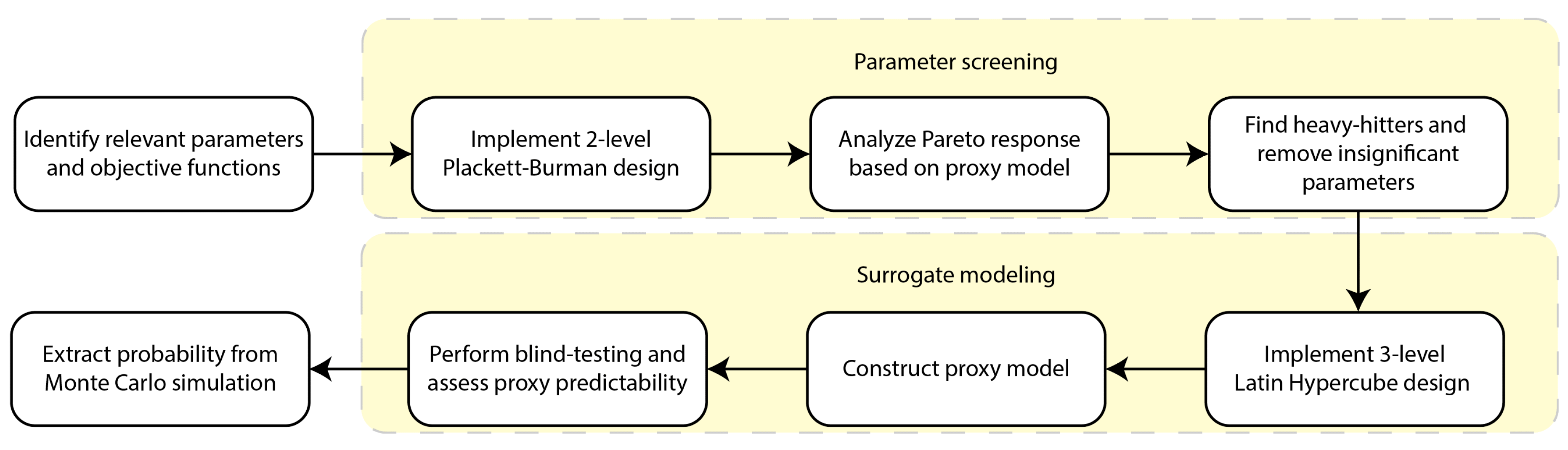
We quantified the performance of the slug-based polymer flooding process using four objective functions, namely, incremental oil recovery over the reference continuous polymer flooding $\left(\Delta R{F}_{cp}{}^{sp}\right)$ at the end of the displacement corresponding to one $PVI$, incremental oil recovery over waterflooding at the end of the displacement $\left(\Delta R{F}_{wf}{}^{sp}\right)$, ratio of the average pressure during slug-based polymer flooding to the average pressure during continuous polymer flooding $\left(P{R}_{cp}{}^{sp}\right)$, and ratio of the average pressure during slug-based polymer flooding to the average pressure during water flooding over the same injection time $\left(P{R}_{wf}{}^{sp}\right)$. Monitoring the average injection pressure is essential to capture any degradation issues in the injectivity.

2.6. DoE Workflow

Here, we describe the overall schematic of the DoE workflow, which follows the work of Santoso et al. [17]. After identifying the relevant parameters and objective functions, as described in the previous two sections, we implemented a parameter screening workflow to identify the heavy-hitters and the insignificant parameters. Then, we proceeded into the surrogate modeling workflow step using only the heavy-hitters. Finally, we extract the probability distributions using Monte Carlo simulations.

3. Results and Discussion

In this section, we report and discuss the results obtained in this study. We start by exploring in detail a test case to explain the recovery mechanisms for the proposed compositionally-tuned slug-based process and to highlight the key differences compared to both the baseline waterflooding and the continuous polymer flooding. Then, we move into the DoE workflow and show the sensitivity of the objective functions to the parameters using two- and three-level Plackett–Burman designs. Finally, we assess the predictive quality of the constructed proxies, which are then used in the Monte Carlo simulations.

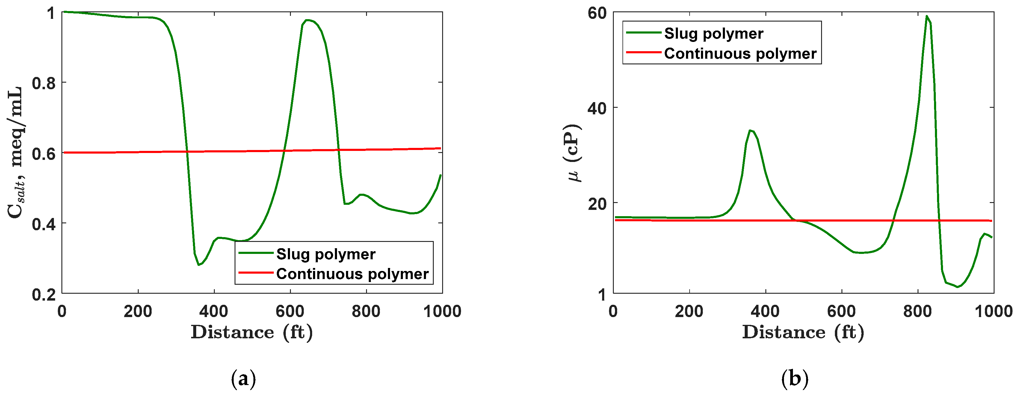
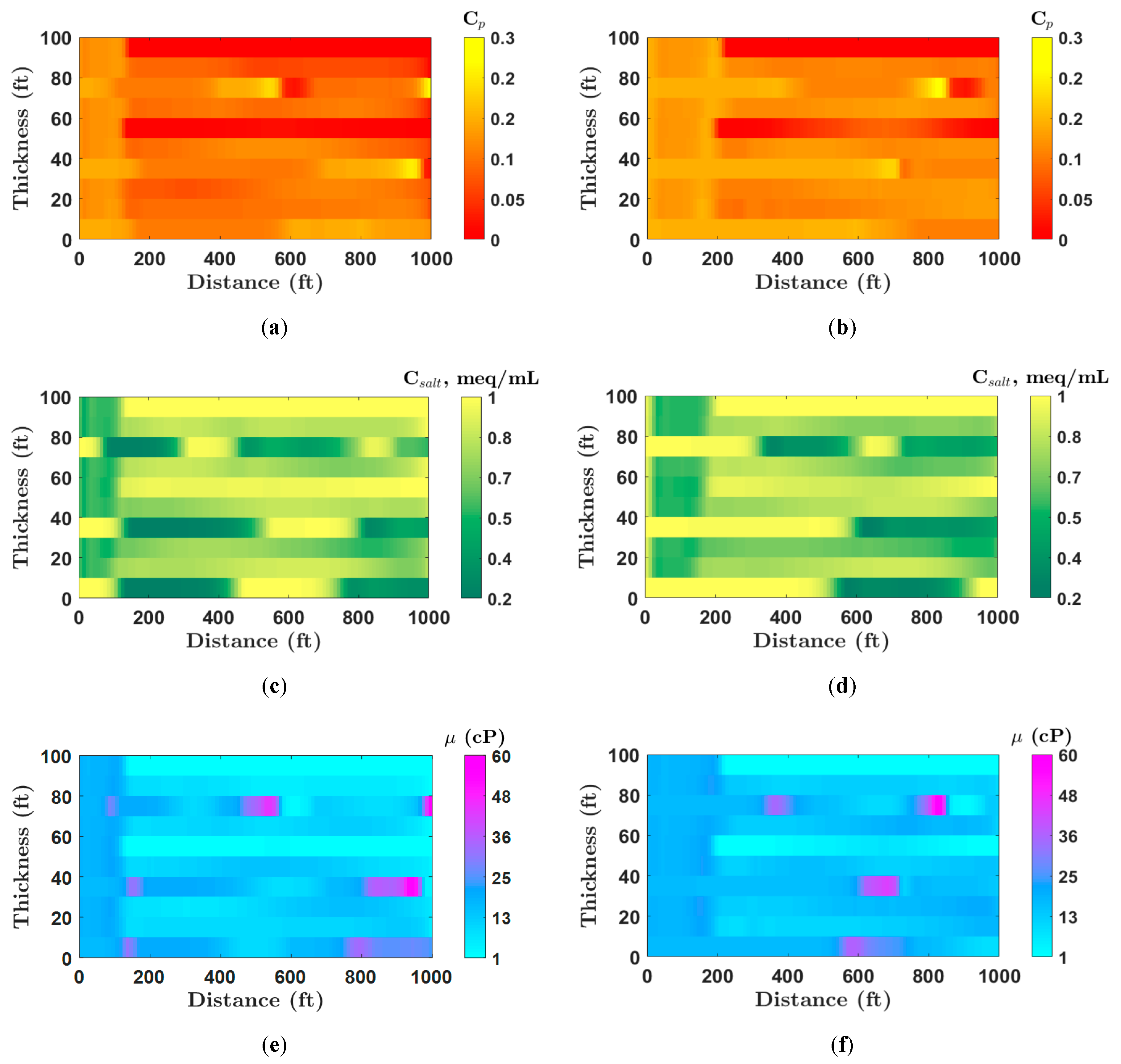
3.1. Recovery Mechanism in the Slug-Based Scheme

The motivation of this test case was to shed more light on the mechanisms governing the proposed slug-based polymer injection scheme, and to emphasize the differences compared to both cases: the continuous polymer flooding and the baseline waterflooding. The parameters corresponding to this test case are listed in the first column of Table 1. Other simulation input parameters are listed in

Table 2. Additional parameters kept constant for all polymer flooding and waterflooding simulations.

$\varphi$	$K_z$, mD	$P_{res}=P_{prod},psia$	$q_{inj},PVI/yr$	$S_w{}^o$	$S_{or}=S_{wr}$
0.28	$0.1K$	1000	0.1	0.2	0.2
$k_{ro}=k_{rw}$	$n_o=n_w$	${\mu }_w$, cP	${\mu }_o$, cP	$S_p$	${\dot{\gamma }}_c,s^{-1}$
0.5	1.5	1	30	-0.5	4
${\dot{\gamma }}_{1/2},s^{-1}$	$P_{\alpha }$	$a_{p2}$, ml/meq	$b_p$, wt.%−1	$b_{RK}$,wt.%−1	$c_{RK}$, D1/2
47	1.7	0.5	100	1.0	0

. The reservoir layers and the corresponding permeabilities are shown in Figure 2.

Figure 3 shows the oil recovery factor (a) and injection bottom hole pressure (b) as a function of pore volumes injected for the three schemes. The continuous and slug-based polymer processes are switched to polymer injection after $t_D=0.75$ of water injection, where $t_D$ is a dimensionless time reflecting $PVI$. The recovery-factor response from switching to polymer becomes pronounced at $t_D=1.0$ (i.e., after injecting 0.25 $PVI$ of polymer), while the pressure response is immediate. From an oil recovery standpoint, the slug-based process yields clear benefits over the continuous process, with cyclical increments corresponding to the cyclical injection of slugs. At $t_D=1.75$ for this test case, the incremental oil recovery was 6% OOIP and 19% OOIP over continuous polymer flooding and waterflooding, respectively. The injection bottom hole pressure for both polymer processes increased between 1.6 to 1.7 times that of waterflooding, owing to the higher aqueous phase viscosity. However, it is important to note that the slug-based process is able to increase oil recovery without impacting injectivity compared to the continuous polymer flood. In this case, the injection bottom hole pressure of the slug-based process increased by only about 5% compared to that of the continuous polymer injection. One interesting feature of the slug-based process is the cyclical nature of the pressure: After the initial increase in pressure, there is a pressure decrease during the injection of the leading slug (i.e., low salinity and polymer concentration) and a pressure increase during the injection of the trailing slug (i.e., high salinity and polymer concentration). The reason for the pressure decrease is the acceleration of the low polymer concentration from the leading slug into the high salinity of the trailing slug from the previous cycle, causing a drop in aqueous phase viscosity. Similarly, the reason for the pressure increase is the acceleration of the high polymer concentration from the trailing slug into the low salinity of the leading slug from the same cycle, causing a rise in aqueous phase viscosity.

Figure 4 shows the oil saturation profiles for the three recovery schemes at $t_D=1.3$ (a,c,e) and $t_D=1.7$ (b,d,f). The saturation for waterflooding shows a preferential sweep in the high permeability layers, and low sweep in the low permeability layers. Figure 5 shows the remaining oil saturations versus distance in layers nine (a) and eight (b), where two different phenomena appear. In layer nine (Figure 5a), the slug-based method shows an improved oil sweep compared to the waterflood baseline and the continuous polymer flood methods. In layer eight (Figure 5b), the slug-based method shows two oil banks, corresponding to the enhanced polymer viscosity from slug mixing. The formation of secondary oil-banks contributes to the overall improvement in the recovery factor. The saturation distribution during the continuous and slug-based polymer injection also suggests that there is an improved crossflow from the high to low permeability layers owing to the increase in aqueous phase viscosity. Figure 6 presents the salinity and viscosity profiles versus distance in layer 8, which highlights the viscosity boost as a result of salinity and polymer concentration slugs.

Figure 7 shows the polymer concentration in wt.% (a,b), salinity (c,d), and aqueous phase viscosity (e,f) profiles at $t_D=1.3$ (a,c,e) and $t_D=1.7$ (b,d,f) for the slug-based process. Figure 8 shows the same profiles for the continuous polymer injection process, provide for comparison. From Figure 7, in the third layer from the top, we note a sharp accumulation in polymer concentration from the trailing slug (a,b) accelerating into low salinity conditions from the leading slug (c,d), responsible for the increase in aqueous phase viscosity (e,f).

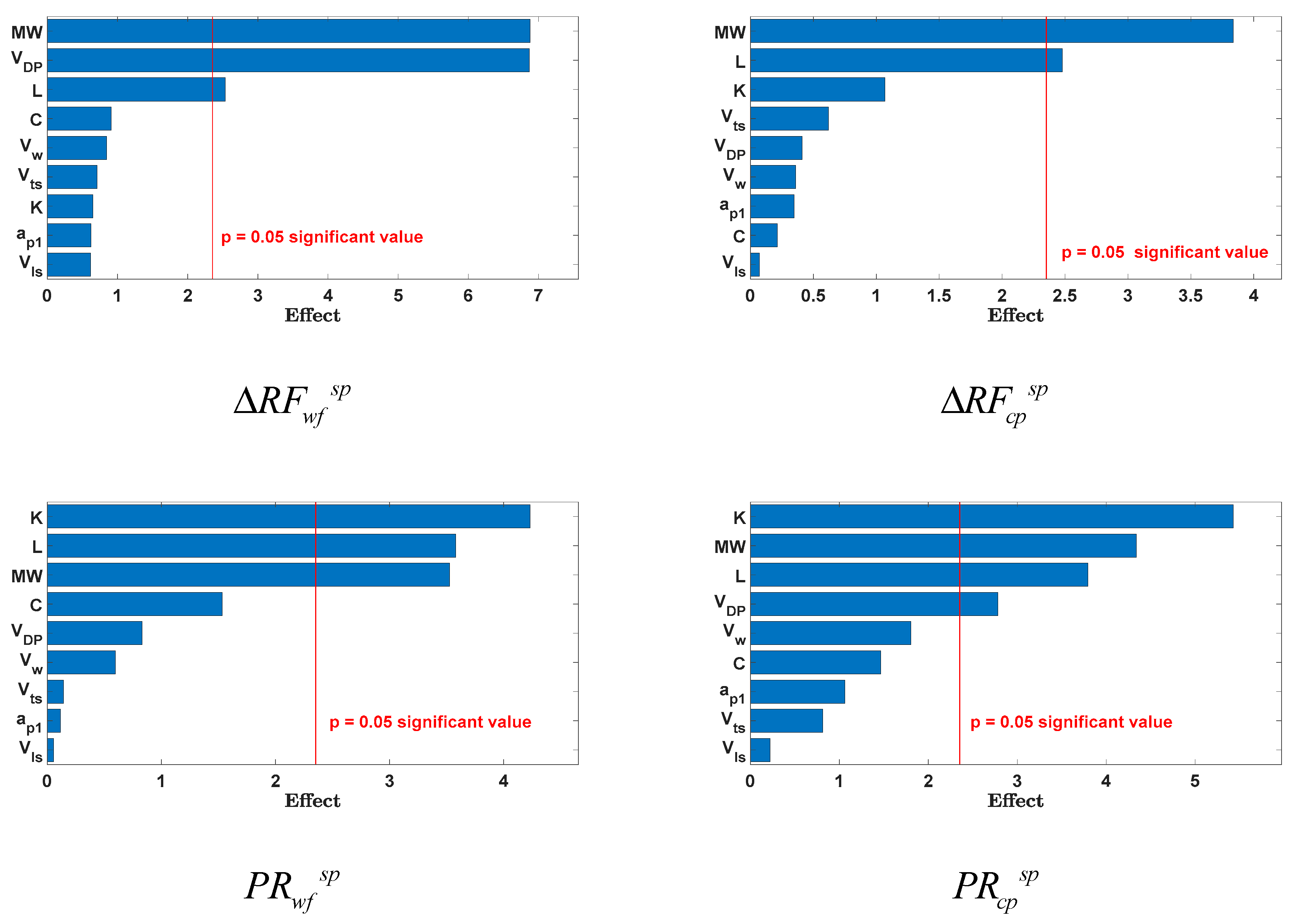
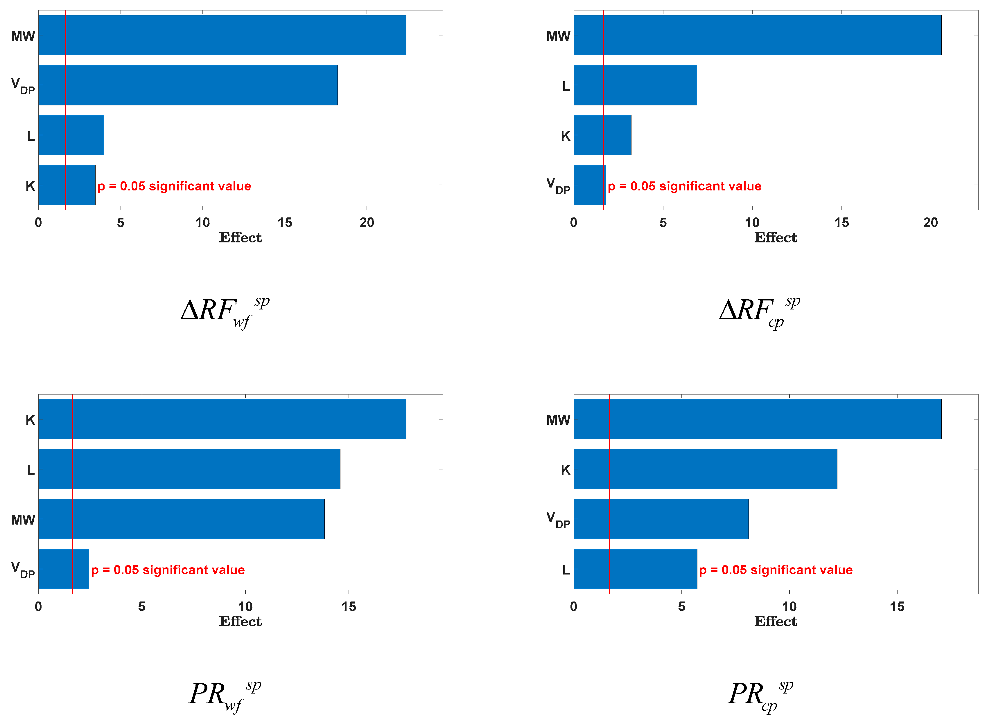
3.2. Parameter Screening

The DoE workflow is described in Figure 9. The first step in the workflow is a screening step to identify the significant parameters by using a two-level Plackett–Burman design. Screening using Plackett–Burman design inherently assumes uniform distribution for all parameters and independency among parameters [53]. Therefore, we had to make sure that parameters or groups of parameters were appropriately arranged, and their correlations to each other were well-investigated. Figure 10 shows a Pareto chart showing the parameter significance relative to the four objective functions described previously. For the incremental oil recovery of the slug-based process over waterflooding, the heavy-hitters are the polymer molecular weight ($MW$), Dykstra–Parsons coefficient $\left(V_{DP}\right)$, and interwell spacing $\left(L\right)$. While the heavy-hitters for the incremental oil recovery of the slug-based process over the continuous polymer flooding scheme are $MW$ and $L$. For the pressure ratio between the slug-based process and waterflooding, the heavy-hitters are $K$, $L$ and $MW$; for the pressure ratio between the slug-based process and continuous polymer flooding, the heavy-hitters are $K$, $MW$, $L$ and $V_{DP}$. From this preliminary parameter screening, we identified two reservoir parameters ($K$ and $V_{DP}$) and two design parameters ($MW$ and $L$) as the most significant parameters that were carried on to the subsequent steps in the DoE workflow. We should emphasize that this sensitivity study reflects the significance of a parameter based on its range of uncertainty, which should not be confused with the significance of the absolute value of the parameter. In other words, a measured quantity with narrow uncertainty, as such, brine salinity will be insignificant in the sensitivity study, which does not mean that salinity is insignificant for polymer flood.

Figure 11 shows the importance of deploying a folded two-level Plackett–Burman design with the identified significant variables. Owing to the better definition of the proxy, we can get a more reliable interpretation of the significant parameters. For the incremental oil recovery of the slug-based process over waterflooding, $K$ was now assessed as significant, and for the pressure ratio between the slug-based process and continuous polymer flooding, the order of significance of the heavy-hitters was changed, with $MW$ being the most critical parameter.

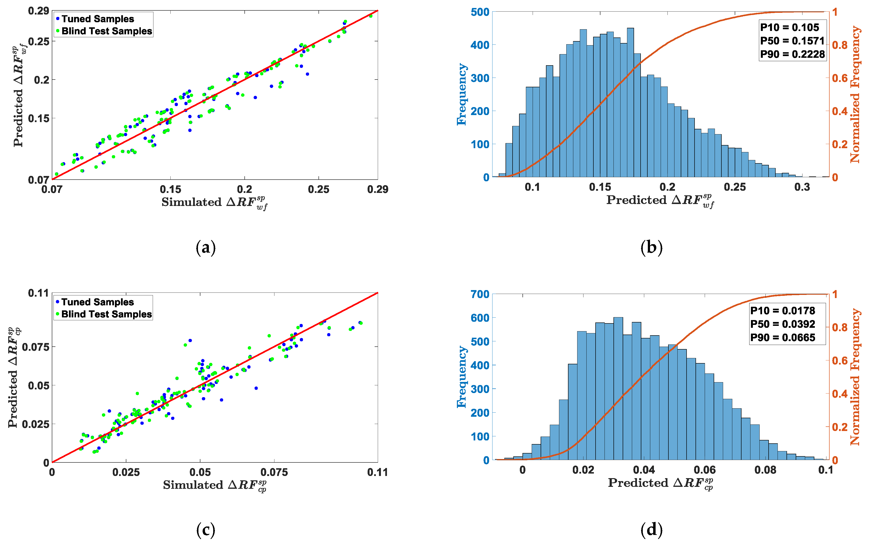
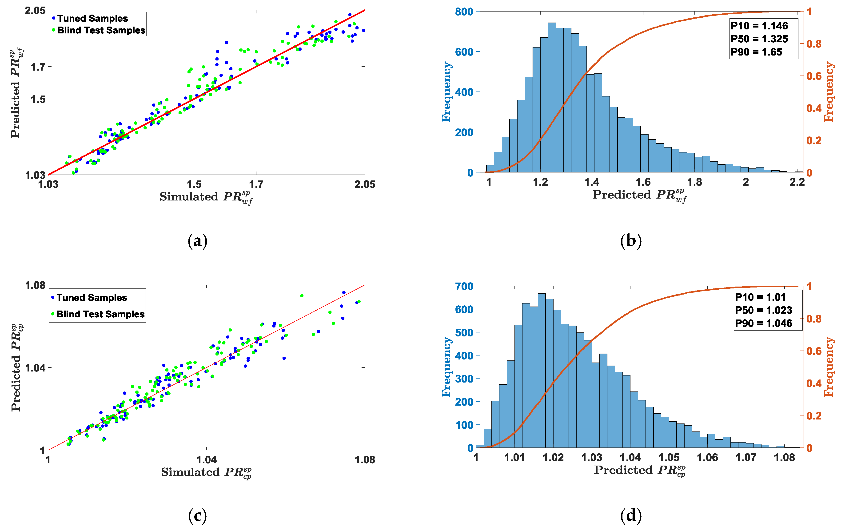
3.3. Uncertainty Quantification

Based on the screened parameters, we proceed into the surrogate modeling (for uncertainty quantification) as part of the DoE workflow. After using a three-level Latin Hypercube design, we tune the proxy parameters using a total of 107 simulation cases. For the proxy modeling step, we consider a quadratic proxy function of the following form

$$F_k={\kappa }^k+{\displaystyle \sum _{i=1}^{N_v}{\kappa }_i{}^k{x}_i}+{\displaystyle \sum _{i,j=1}^{N_v}{\kappa }_{ij}{}^k{x}_i{x}_j,}$$

(8)

where $F_k$ is the objective function, $x_i$ is a proxy variable, $N_v$ is the number of variables, and ${\kappa }^k,{\kappa }_i{}^k$ and ${\kappa }_{ij}{}^k$ are the corresponding regression coefficients. In the cases considered in Equation (5), $\left(F_1,F_2,F_3,F_4\right)$ correspond to $\left(\Delta R{F}_{wf}{}^{sp},\Delta R{F}_{cp}{}^{sp},P{R}_{wf}{}^{sp},P{R}_{cp}{}^{sp}\right)$, based on the parameter screening $N_v=4$, and $\left(x_1,x_2,x_3,x_4\right)$ are the variables corresponding to $\left(L,V_{DP},K,MW\right).$ The corresponding proxy coefficients are listed in

Table 3. Proxy coefficients for the various objective functions considered.

Coefficient	${\mathit{F}}_1$	${\mathit{F}}_2$	${\mathit{F}}_3$	${\mathit{F}}_4$
${\kappa }^k$	0.1573	0.0447	1.0275	1.3762
${\kappa }_1{}^k$	0.0095	0.0118	0.0065	0.1828
${\kappa }_2{}^k$	−0.0470	−0.0020	0.0079	0.0126
${\kappa }_3{}^k$	−0.0096	−0.0063	−0.0147	−0.2604
${\kappa }_4{}^k$	0.0577	0.0291	0.0173	0.1772
${\kappa }_{12}{}^k$	0.0013	0.0014	0.0000	0.0029
${\kappa }_{13}{}^k$	−0.0071	−0.0028	−0.0035	−0.1188
${\kappa }_{14}{}^k$	0.0052	0.0043	−0.0030	−0.0121
${\kappa }_{23}{}^k$	0.0053	0.0036	0.0002	0.0793
${\kappa }_{24}{}^k$	−0.0155	0.0056	0.0090	0.0179
${\kappa }_{34}{}^k$	−0.0016	−0.0043	−0.0078	−0.1003
${\kappa }_{11}{}^k$	0.0003	−0.0002	−0.0011	−0.0082
${\kappa }_{22}{}^k$	0.0150	−0.0122	−0.0021	0.0207
${\kappa }_{33}{}^k$	0.0013	0.0006	0.0026	0.0953
${\kappa }_{44}{}^k$	−0.0034	0.0032	0.0034	−0.0127

F = objective function, $\kappa$ = regression coefficient

.

To verify the proxy predictability, we performed blind testing with 107 random cases. Once we assessed the performance of the proxies, we proceeded into the Monte Carlo simulation, where 10,000 cases were considered to explore the probabilities of the objective functions.

Figure 12a shows a very good agreement between the simulated and predicted values for the incremental oil recovery for the slug-based process over both waterflooding (a,b) and continuous polymer flooding (c,d), with $R^2$ values of 0.93 and 0.91, respectively. More importantly, for all cases considered, $\Delta R{F}_{cp}{}^{sp}>0$, emphasizing that the proposed technology always outperformed the traditional continuous polymer flooding. Monte Carlo simulations (Figure 12b,d) applied to these proxies yielded a most likely (i.e., p50) incremental value for the slug-based process over waterflooding of 16% OOIP and over continuous polymer flooding of 4% OOIP.

Figure 13a,c also shows a good agreement between the simulated and predicted values for the injection pressure ratio of the slug-based process compared to both waterflooding (a,b) and continuous polymer flooding (c,d), with $R^2$ values of 0.94 and 0.93, respectively. For all cases considered, $P{R}_{cp}{}^{sp}$ was slightly above one, emphasizing that the proposed slug-based scheme does not exhibit any major loss in injectivity compared to the continuous polymer flooding scheme. Monte Carlo simulations (Figure 13b,d), using these proxies, yielded a most likely (p50) pressure ratio value of the slug-based process compared to a waterflooding of 1.3, and compared to continuous polymer flooding of 1.02.

4. Summary

In this paper, we evaluated the performance of a new compositionally-tuned slug-based polymer flooding injection scheme using Design-of-Experiments. The recovery performance of the new scheme was compared to both traditional polymer flooding using constant composition injection and baseline waterflooding. The following points summarize the key findings of our study:

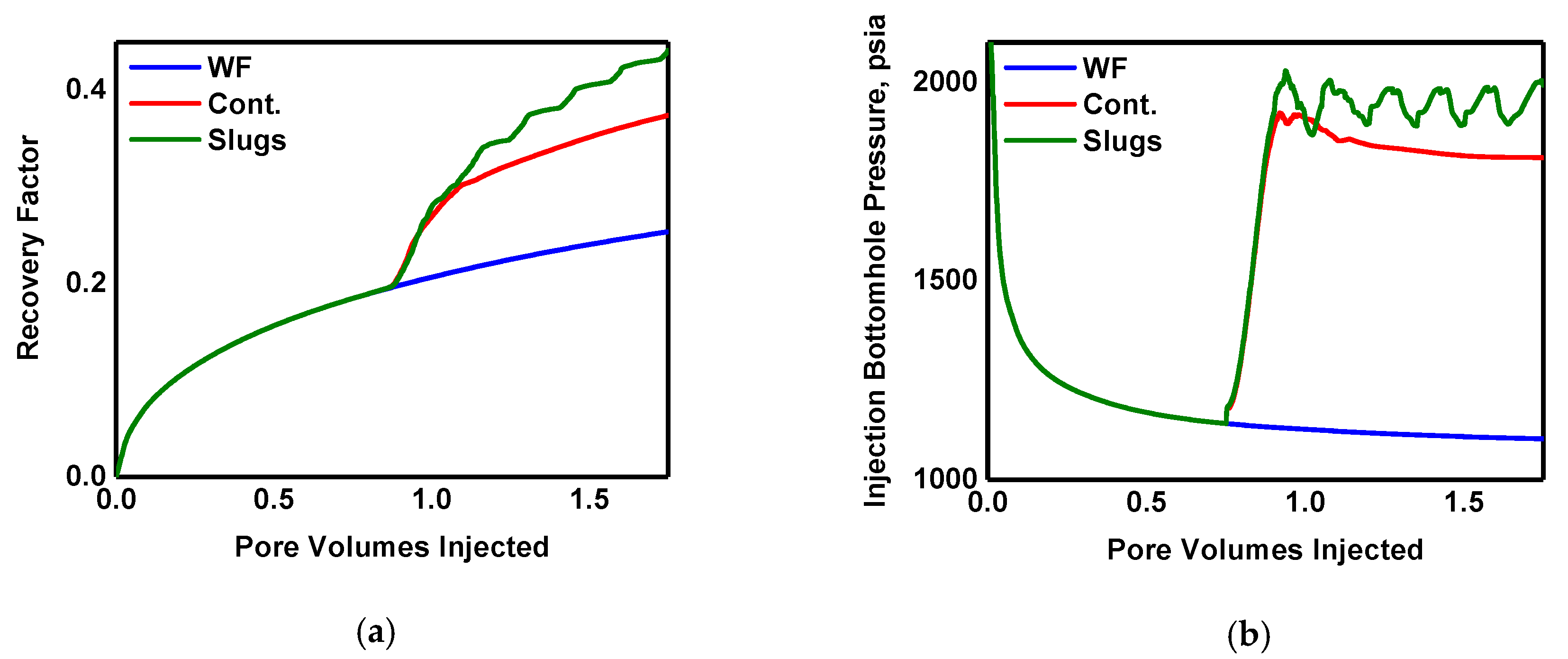
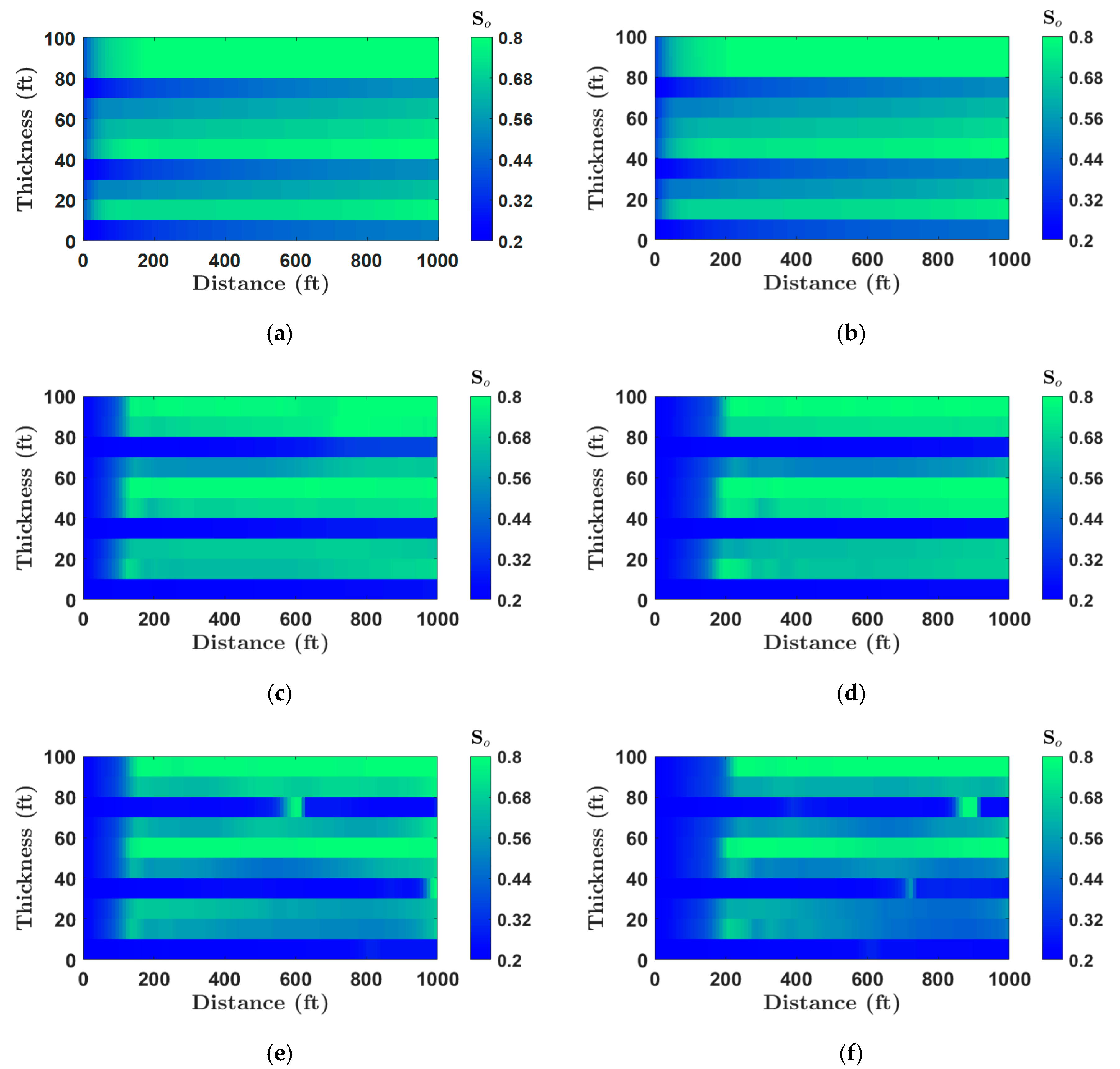
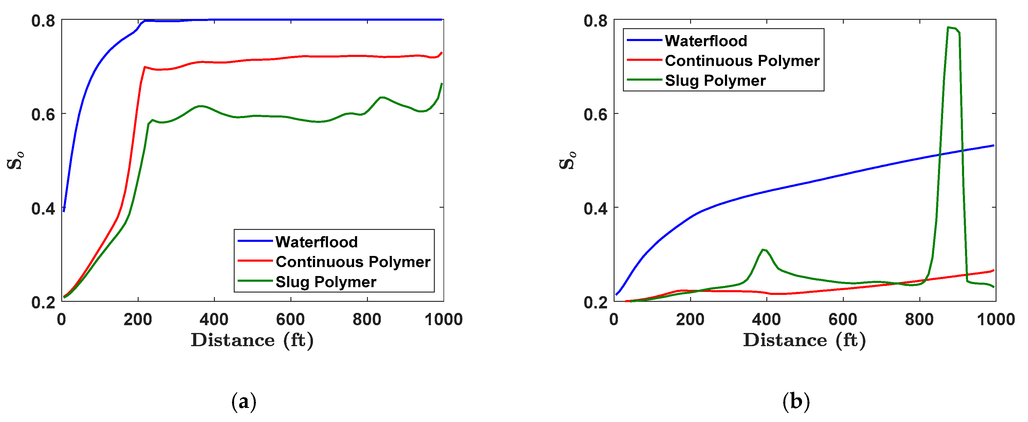
• The new slug-based polymer injection scheme is demonstrated using simulations to increase oil recovery over traditional polymer flooding for all cases considered, without hampering polymer injectivity. This injection scheme leads to a higher recovery factor relative to traditional continuous polymer injection without a need to increase the total mass of the polymer.
• The polymer molecular weight, which controls both the inaccessible pore volume and the polymer viscosity coefficients, was found to be the most critical design parameters. High molecular weight polymer yielded the largest polymer component acceleration over the salinity component, which is responsible for the size of the transition zone.
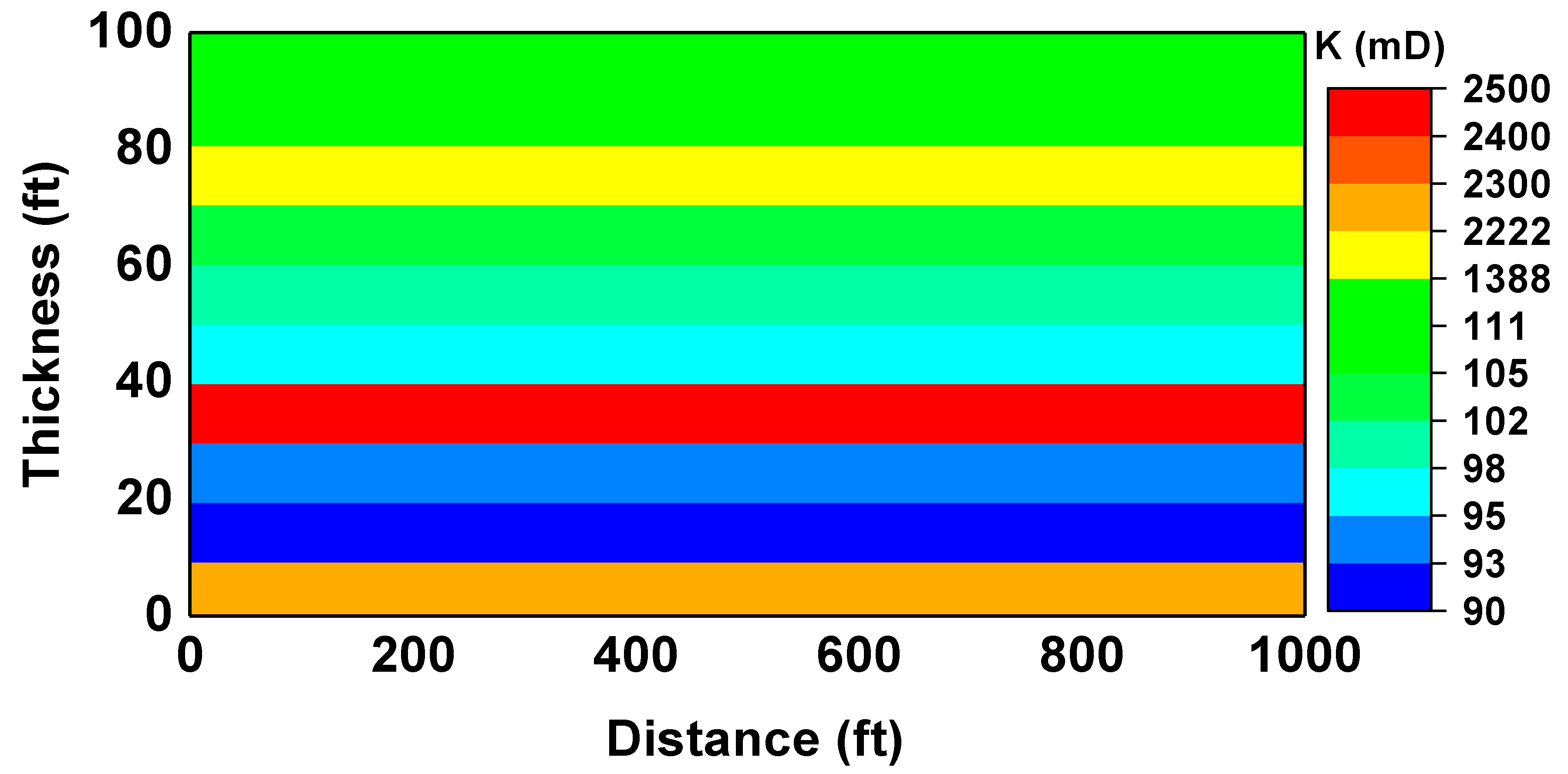
• Vertical heterogeneity was also an important reservoir parameter that impacted the recovery performance. High reservoir heterogeneity increased mixing owing to changes in vertical velocity, which negatively impacted the performance of the recovery process.
• For the ranges considered, polymer adsorption did not play a significant role in the process performance. This behavior is expected because the cases corresponded to rocks with low to moderate adsorption, and hence polymer adsorption, which contributes to polymer component retardation, is satisfied early in the polymer injection process.
• Uncertainty quantification through surrogate modeling can be a useful, yet simple tool to estimate the process performance in the early stages of technology assessment provided that the correct parameters and objective functions are identified.

References

1. Lake, L.; Johns, R.; Rossen, B.; Pope, G. Fundamentals of Enhanced Oil Recovery; Society of Petroleum Engineers: Richardson, TX, USA, 2014. [Google Scholar]
2. Ekkawong, P.; Han, J.; Olalotiti-Lawal, F.; Datta-Gupta, A. Multiobjective design and optimization of polymer flood performance. J. Pet. Sci. Eng. 2017, 153, 47–58. [Google Scholar] [CrossRef] [Green Version]
3. Torrealba, V.A.; Hoteit, H. Improved polymer flooding injectivity and displacement by considering compositionally-tuned slugs. J. Pet. Sci. Eng. 2019, 178, 14–26. [Google Scholar] [CrossRef]
4. Bowman, K.P.; Sacks, J.; Chang, Y.-F. Design and analysis of numerical experiments. J. Atmos. Sci. 1993, 50, 1267–1278. [Google Scholar] [CrossRef] [Green Version]
5. Leray, S.; Douarche, F.; Tabary, R.; Peysson, Y.; Moreau, P.; Preux, C. Multi-objective assisted inversion of chemical EOR corefloods for improving the predictive capacity of numerical models. J. Pet. Sci. Eng. 2016, 146, 1101–1115. [Google Scholar] [CrossRef]
6. Antony, J. Design of Experiments for Engineers and Scientists, 2nd ed.; Elsevier Ltd.: Burlington, MA, USA, 2014; ISBN 9780080994178. [Google Scholar]
7. Fisher, R.A. Studies in crop variation: I. An examination of the yield of dressed grain from broadbalk. J. Agric. Sci. 1921, 11, 107–135. [Google Scholar] [CrossRef] [Green Version]
8. Fisher, R.A. Theory of Statistical Estimation. Math. Proc. Camb. Philos. Soc. 1925, 22, 700–725. [Google Scholar] [CrossRef] [Green Version]
9. Sawyer, D.N.; Cobb, W.M.; Stalkup, F.I.; Braun, P.H. Factorial Design Analysis of Wet-Combustion Drive. Soc. Pet. Eng. J. 1974, 14, 25–34. [Google Scholar] [CrossRef]
10. Damsleth, E.; Hage, A.; Volden, R. Maximum information at minimum cost: A north sea field development study with an experimental design. J. Pet. Technol. 1992, 44, 1350–1356. [Google Scholar]
11. Friedmann, F.; Chawathe, A.; Larue, D.K. Assessing uncertainty in channelized reservoirs using Experimental Designs. SPE Reserv. Eval. Eng. 2003, 6, 264–274. [Google Scholar] [CrossRef]
12. Ghaderi, S.M.; Clarkson, C.R.; Chen, S. Optimization of WAG process for coupled CO2 EOR-storage in tight oil formations: An experimental design approach. In Proceedings of the SPE Canadian Unconventional Resources Conference, Calgary, AB, Canada, 30 October–1 November 2012. [Google Scholar]
13. Ogunbanwo, O.; Gerritsen, M.; Kovscek, A.R. Uncertainty analysis on in-situ combustion simulations using experimental design. In Proceedings of the Society of Petroleum Engineers Western Regional Meeting, San Jose, CA, USA, 23–26 April 2012; pp. 599–612. [Google Scholar]
14. Bevillon, D.; Mohagerani, S. Miscible EOR project in a mature, offshore, carbonate middle east reservoir-Uncertainty analysis with proxy models based on experimental design of reservoir simulations. In Proceedings of the SPE Reservoir Characterisation and Simulation Conference and Exhibition, Abu Dhabi, UAE, 14–16 September 2015; Society of Petroleum Engineers: Houston, TX, USA, 2015; pp. 752–775. [Google Scholar]
15. Bengar, A.; Moradi, S.; Ganjeh-Ghazvini, M.; Shokrollahi, A. Optimized polymer flooding projects via combination of experimental design and reservoir simulation. Petroleum 2017, 3, 461–469. [Google Scholar] [CrossRef]
16. Adepoju, O.O.; Hoteit, H.; Chawathe, A. Assessment of chemical performance uncertainty in chemical EOR simulations. In Proceedings of the Society of Petroleum Engineers—SPE Reservoir Simulation Conference 2017, Montgomery, TX, USA, 20–22 February 2017; Society of Petroleum Engineers: Houston, TX, USA, 2017; pp. 127–140. [Google Scholar]
17. Santoso, R.; Hoteit, H.; Vahrenkamp, V. Optimization of energy recovery from geothermal reservoirs undergoing re-injection: Conceptual application in Saudi Arabia. In Proceedings of the SPE Middle East Oil and Gas Show and Conference, Manama, Bahrain, 18–21 March 2019; Society of Petroleum Engineers (SPE): Houston, TX, USA, 2019. [Google Scholar]
18. Ram, M.; Delshad, M. A Compositional Reservoir Simulator on Distributed Memory Parallel Computers. In Proceedings of the SPE Reservoir Simulation Symposium, San Antonio, TX, USA, 12–15 February 1995. [Google Scholar]
19. Zhang, J.; Delshad, M.; Sepehrnoori, K.; Pope, G.A. An Efficient Reservoir-Simulation Approach To Design and Optimize Improved Oil-Recovery-Processes With Distributed Computing. In Proceedings of the SPE Latin American and Caribbean Petroleum Engineering Conference, Bogotá, Colombia, 17–19 March 2005; Society of Petroleum Engineers: Houston, TX, USA, 2005. [Google Scholar]
20. Zhang, J.; Delshad, M.; Sepehrnoori, K. A Framework to Design and Optimize Surfactant-Enhanced Aquifer Remediation. In Proceedings of the SPE/EPA/DOE Exploration and Production Environmental Conference, Galveston, TX, USA, 7–9 March 2005; Society of Petroleum Engineers: Houston, TX, USA, 2005. [Google Scholar]
21. UTCHEM-9.0 Technical Documentation; The University of Texas at Austin: Austin, TX, USA, 2000.
22. Liauh, W.C.; Duda, J.L.; Klaus, E.E. An Iinvestigation of the Inaccessible Pore Volume Phenomena. In Proceedings of the 84th National American Institute of Chemical Engineers Meeting, Atlant, GA, USA, 28 Februray–1 March 1978. [Google Scholar]
23. Dawson, R.; Lantz, R.B. Inaccesible Pore Volume in Polymer Flooding. SPE J. 1972, 12, 448–452. [Google Scholar]
24. Pancharoen, M. Physical Properties of Associative Polymer Solutions; Stanford University: Stanford, CA, USA, 2009. [Google Scholar]
25. Pancharoen, M.; Thiele, M.R.; Kovscek, A.R. Inaccessible Pore Volume of Associative Polymer Floods. In Proceedings of the SPE Improved Oil Recovery Symposium, Tulsa, OK, USA, 24–28 April 2010; Society of Petroleum Engineers: Houston, TX, USA, 2010. [Google Scholar]
26. De Gennes, P.G. Dynamics of Entangled Polymer Solutions. I. The Rouse Model. Macromolecules 1976, 9, 587–593. [Google Scholar] [CrossRef]
27. De Gennes, P.G. Dynamics of Entangled Polymer Solutions. II. Inclusion of Hydrodynamic Interactions. Macromolecules 1976, 9, 594–598. [Google Scholar] [CrossRef]
28. Nouri, H.H.; Root, P.J. A Study of Polymer Solution Rheology, Flow Behavior, and Oil Displacement Processes. In Proceedings of the Fall Meeting of the Society of Petroleum Engineers of AIME, Cincinnati, OH, USA, 19–21 January 1971; Society of Petroleum Engineers: Houston, TX, USA, 1971. [Google Scholar]
29. Szabo, M.T. Molecular and Microscopic Interpretation of the Flow of Hydrolyzed Polyacrylamide Solution Through Porous Media. In Proceedings of the Fall Meeting of the Society of Petroleum Engineers of AIME, San Antonio, TX, USA, 8–11 October 1972; Society of Petroleum Engineers: Houston, TX, USA, 1972. [Google Scholar]
30. Hirasaki, G.J.; Pope, G.A. Analysis of Factors Influencing Mobility and Adsorption in the Flow of Polymer Solution Through Porous Media. Soc. Pet. Eng. J. 1974, 14, 337–346. [Google Scholar] [CrossRef]
31. Maerker, J.M. Shear Degradation of Partially Hydrolyzed Polyacrylamide Solutions. Soc. Pet. Eng. J. 1975, 15, 311–322. [Google Scholar] [CrossRef]
32. Szabo, M.T. Laboratory Investigations of Factors Influencing Polymer Flood Performance. Soc. Pet. Eng. J. 1975, 15, 338–346. [Google Scholar] [CrossRef]
33. Forsman, W.C.; Hughes, R.E.; Forsmant, W.C. Adsorption of Polymer Molecules at Low Surface Coverage. J. Chem. Phys. 1963, 38, 2558. [Google Scholar]
34. Dominguez, J.G.; Willhite, G.P. Retention and Flow Characteristics of Polymer Solutions in Porous Media. Soc. Pet. Eng. J. 1977, 17, 111–121. [Google Scholar] [CrossRef]
35. Delshad, M.; Pope, G.A.; Sepehrnoori, K. A compositional simulator for modeling surfactant enhanced aquifer remediation, 1 Formulation. J. Contam. Hydrol. 1996, 23, 303–327. [Google Scholar] [CrossRef]
36. Ahmed, H.; Glass, J.E.; McCarthy, G.J. Adsorption of Water-Soluble Polymers on High Surface Area Clays. In Proceedings of the SPE Annual Technical Conference and Exhibition, San Antonio, TX, USA, 4–7 October 1981; Society of Petroleum Engineers: Houston, TX, USA, 1981. [Google Scholar]
37. Krebs, H.J. Wilmington Field, California, Polymer Flood—A Case History. J.Pet. Technol. 1976, 28, 1473–1480. [Google Scholar] [CrossRef]
38. Shuler, P.J.; Kuehne, D.L.; Uhl, J.T.; Walkup, G.W. Improving Polymer Injectivity at West Coyote Field, California. SPE Reserv. Eng. 1987, 2, 271–280. [Google Scholar] [CrossRef]
39. Darcy, H. Les Fontaines Publiques de la Ville de Dijon; Librairie Des Corps Impérial Des Ponts et Chaussees et Des Mines: Paris, France, 1856. [Google Scholar]
40. Pope, G.A.; Hong, C.H.; Sepehrnoori, K.; Lake, L.W. Two Dimensional Simulation of Chemical Flooding. In Proceedings of the SPE California Regional Meeting, Bakersfield, CA, USA, 25–27 March 1981; Society of Petroleum Engineers: Houston, TX, USA, 1981. [Google Scholar]
41. Lake, L.W.; Johnston, J.R.; Stegemeir, G.L. Simulation and Performance Prediction of A Large-Scale Surfactant/Polymer Project. Soc. Pet. Eng. J. 1981, 21, 731–739. [Google Scholar] [CrossRef]
42. Jensen, J.L.; Hinkley, D.V.; Lake, L.W. Statistical Study of Reservoir Permeability: Distributions, Correlations, and Averages. SPE Form. Eval. 1987, 2, 461–468. [Google Scholar] [CrossRef]
43. Wang, J.; Wang, D.; Sui, X.; Zeng, H.; Bai, W. Combining Small Well Spacing With Polymer Flooding to Improve Oil Recovery of Marginal Reservoirs. In Proceedings of the SPE/DOE Symposium on Improved Oil Recovery, Tulsa, OK, USA, 22–26 April 2006; Society of Petroleum Engineers: Houston, TX, USA, 2006. [Google Scholar]
44. Wang, D.; Dong, H.; Lv, C.; Fu, X.; Nie, J. Review of practical experience of polymer flooding at Daqing. SPE Reserv. Eval. Eng. 2009, 12, 470–476. [Google Scholar] [CrossRef]
45. Hughes, D.S.; Teeuw, D.; Cottrell, C.W.; Tollas, J.M. Appraisal of the use of polymer injection to suppress aquifer influx and to improve volumetric sweep in a viscous oil reservoir. SPE Reserv. Eng. 1990, 5, 33–40. [Google Scholar] [CrossRef]
46. Wisniewska, A.; Sozanski, K.; Kalwarczyk, T.; Kedra-Krolik, K.; Holyst, R. Scaling Equation for Viscosity of Polymer Mixtures in Solutions with Application to Diffusion of Molecular Probes. Macromolecules 2017, 50, 4555–4561. [Google Scholar] [CrossRef]
47. Delamaide, E.; Technologies, I.F.P.; Tabary, R.; Rousseau, D.; Energies, I.F.P. SPE-169673-MS Chemical EOR in Low Permeability Reservoirs. In Proceedings of the SPE EOR Conference at Oil and Gas West Asia, Muscat, Oman, 31 March–2 April 2014; Volume 1963, pp. 1–15. [Google Scholar]
48. Jensen, J.L.; Lake, L.W.; Corbett, P.W.M.; Goggin, D.J. Statistics for Petroleum Engineers and Geoscientists; Elsevier: Amsterdam, The Netherlands, 1997. [Google Scholar]
49. Hoteit, H.; Chawathe, A. Making field-scale chemical enhanced-oil-recovery simulations a practical reality with dynamic gridding. SPE J. 2016, 21. [Google Scholar] [CrossRef]
50. Najafabadi, N.F.; Chawathe, A. Proper Simulation of Chemical EOR (CEOR) Pilots—A Real Case Study. In Proceedings of the SPE Improved Oil Recovery Conference, Tulsa, OK, USA, 9–13 April 2016; Society of Petroleum Engineers: Houston, TX, USA, 2016. [Google Scholar]
51. Naik, P.; Pandita, P.; Aramideh, S.; Bilionis, I.; Ardekani, A.M. Bayesian model calibration and optimization of surfactant-polymer flooding. Comput. Geosci. 2019, 23, 981–996. [Google Scholar] [CrossRef]
52. Torrealba, V.A.; Hoteit, H.; Chawathe, A. Improving Chemical-Enhanced-Oil-Recovery Simulations and Reducing Subsurface Uncertainty Using Downscaling Conditioned to Tracer Data. SPE Reserv. Eval. Eng. 2019, 22. [Google Scholar] [CrossRef]
53. Li, H.; Sarma, P.; Zhang, D. A comparative study of the probabilistic-collocation and experimental-design methods for petroleum-reservoir uncertainty quantification. SPE J. 2011, 16, 429–439. [Google Scholar] [CrossRef]
Figure 1. Illustration showing how the compositionally-tuned slug-based polymer flooding scheme works: Owing to polymer acceleration, a transition zone forms between the leading and trailing slugs, where polymer solution viscosity is significantly higher than the injected viscosities. The zones on the left, middle, and right correspond, respectively to high-salinity-high-polymer (HSHP) concentration (trailing slug), low salinity-high polymer (LSHP) concentration (mixing zone), low-salinity-low-polymer (LSLP) concentration (leading slug).
Processes 08 00197 g001
Figure 2. Vertical cross-section of the reservoir model showing the layering and the corresponding permeabilities for the test case with V D P = 0.7 and K = 681 m D .
Processes 08 00197 g002
Figure 3. Oil recovery factor (a) and injection bottom hole pressure (b) as a function of pore volumes injected for the test case using waterflooding (WF), continuous polymer flooding (Cont.), and the compositionally-tuned slug-based process (Slugs).
Processes 08 00197 g003
Figure 4. Oil saturation profiles for the test case using waterflooding (a,b), continuous polymer flooding (c,d), and the compositionally-tuned slug-based process (e,f) at t D = 1.3 (a,c,e) and t D = 1.7 (b,d,f).
Processes 08 00197 g004
Figure 5. Oil saturation profiles for the test case in layer nine (a), and layer eight (b) at t D = 1.7 .
Processes 08 00197 g005
Figure 6. Water salinity (a), and aqueous phase viscosity (b) profiles versus distance for the slug-based (green) and continuous (red) polymer schemes in layer eight (middle) at t D = 1.7 .
Processes 08 00197 g006
Figure 7. Polymer concentration in wt.% (a,b), salinity (c,d), and aqueous phase viscosity (e,f) profiles for the test case using the compositionally-tuned slug-based process at t D = 1.3 (a,c,e) and t D = 1.7 (b,d,f).
Processes 08 00197 g007
Figure 8. Polymer concentration (a,b), salinity (c,d), and aqueous phase viscosity (e,f) profiles for the test case using the continuous polymer flooding scheme at t D = 1.3 (a,c,e) and t D = 1.7 (b,d,f).
Processes 08 00197 g008
Figure 9. Simplified schematic showing the overall Design of Experiments workflow used in this paper, following the recent work of Santoso et al. (2019).
Processes 08 00197 g009
Figure 10. Pareto chart for the selected objective functions using a folded two-level Plackett–Burman design as part of the parameter screening workflow. Parameters with an effect less than the red line are considered insignificant, and more than the red line are considered heavy-hitters.
Processes 08 00197 g010
Figure 11. Pareto chart for the selected objective functions using a folded two-level Plackett–Burman design as part of the surrogate modeling workflow. Parameters with an effect less than the red line are considered insignificant, and more than the red line are considered heavy-hitters.
Processes 08 00197 g011
Figure 12. Assessment of proxy quality as part of the surrogate modeling workflow (a,c) and resulting probabilities from the Monte Carlo simulation (b,d) for the incremental oil recovery of the slug-based process over waterflooding (a,b), and over continuous polymer flooding (c,d).
Processes 08 00197 g012
Figure 13. Assessment of proxy quality as part of the surrogate modeling workflow (a,c) and resulting probabilities from the Monte Carlo simulation (b,d) for the average injection bottom hole pressure ratio of the slug-based process to waterflooding (a,b), and to continuous polymer flooding (c,d).
Processes 08 00197 g013