Article

Phenomenological Analysis of Thermo-Mechanical-Chemical Properties of GFRP during Curing by Means of Sensor Supported Process Simulation

German Aerospace Center (DLR), Lilienthalplatz 7, 38108 Braunschweig, Germany
*
Author to whom correspondence should be addressed.
These authors contributed equally to this work.
Processes 2020, 8(2), 192; https://doi.org/10.3390/pr8020192
Submission received: 31 December 2019 / Revised: 25 January 2020 / Accepted: 30 January 2020 / Published: 5 February 2020
(This article belongs to the Special Issue Synergies in Combined Development of Processes and Models)

Abstract

:
Inherent process-induced deformations (PID) and residual stresses impede the application of composite parts. PID lead to a geometrical mismatch in assemblies and require subsequent work for tolerance compensation. Unknown residual stresses cause overweighted structures resulting from unnecessary high safety factors. To counteract the deformations, the tool design needs to be modified until the component geometry meets the specifications. This process is mostly carried out empirically and is time and cost intensive. To improve the efficiency of the development process, an in-deep comprehension of the manufacturing processes is mandatory. Therefore, experimental and simulation-based methods are increasingly applied and enhanced. The object of this work is to investigate the development of process-induced strains as well as the material behaviour during the manufacturing for a GFRP plate. The process-induced strains are monitored by optical fiber Bragg grating (FBG) sensors. The change of the material phases is detected by dielectric sensors. Furthermore, a detailed process simulation considering viscoelastic effects and reaction kinetics is performed. Finally, the measurements are correlated with the simulation data to validate the simulation approach. A very good correlation for both the reaction kinetics as well as the process-induced strains is observed.

1. Introduction

Fibre-reinforced plastics (FRP) are increasingly applied for weight savings due to their high weight-specific stiffness and strength ratio. The high stiffness and strength in fiber direction enable a tailored design according to the load path. Composite components are often manufactured by a differential design which corresponds to the metallic design method. Here, parts with simple geometries are assembled to complex subcomponents. The main advantages are simple tooling geometries and low process risks [1]. On the other hand, the manufacturing costs are quite high due to the cost-intensive joining and assembling processes. Furthermore, a differential design is not a fiber-oriented design and the high potential of the material is not utilized. Using an integral design approach a fiber-oriented design can be achieved at reduced manufacturing costs. However, such an approach leads to a higher process risk. During manufacturing, inherent process-induced residual stresses and resulting deformations occur. They occur due to different thermal and mechanical properties of the fiber and matrix material as well as due to different material orientations of adjacent plies. The deformations may exceed predefined tolerances and parts cannot be assembled. Subsequent work for tolerance compensation is necessary in order to ensure a lean assembly. This leads to increased manufacturing costs and lower production rates.
Residual stresses effect the strength and can influence the failure behaviour [2,3,4]. Furthermore, they can initiate cracks in the fiber–matrix interface which can result in delamination and premature component failure [2]. The stresses depend on the process history and can be influenced by the curing process itself [5,6]. In the initial state, the matrix usually behaves like a liquid. By the introduction of energy in form of elevated temperatures the curing process is activated. Short-chain epoxy molecules are cross-linked via polymerisation to increasingly longer polymer chains, forming a tight three-dimensional network. After the formation of a wide-meshed network, the material gels and the material behaviour changes from a liquid to a rubbery state. The time of the transition is called the gel point. From this point, stress transfer inside as well as into the material is possible. As the curing process proceeds the polymer network increases. Finally, the material changes from a rubbery state to a glassy state. The transition is called vitrification. Thereby, the stiffness increases and process-induced strains are stored as frozen-in strains. During the cool down from the curing temperature to room temperature thermal stresses arise. The Young’s modulus and the shear modulus in the rubber–elastic state are ~100 times lower and the coefficient of thermal expansion (CTE) approximately two to three times higher than in the glass-like state [7]. This means that the final stress state and the level of stresses depend strongly on the gel point.
The different material phases and the changing material properties during the curing process show that the consideration of the entire process history is a crucial aspect in the part development process. To ensure robust processes, an in-deep comprehension of the manufacturing process is mandatory. The object of the work is to investigate the development of process-induced strains and the change of material properties during the manufacturing process. Therefore, an experimental as well as a numerical analysis are performed. The process-induced strains, in the following abbreviated as process strains, are monitored by optical fiber Bragg grating (FBG) sensors. The optical sensors are already successfully applied in different papers [8,9,10] for the real-time measurement of process strains. Oliveira et al. [8] used embedded FBG sensors to investigate the influence of the mould material on the residual strains in the structure. As a result, the largest residual strains were found for the samples cured on aluminium or steel moulds. In this work a steel mould is used. Nielsen [9] measured the process strains of a thick glass/epoxy cross-ply laminate and compared the results to process simulations using the linear–elastic CHILE model proposed by Johnston [11] and the simplified visco-elastic model proposed by Svanberg [7]. A good correlation between simulations and measurements could be found. In order to consider also visco-elastic effects and to improve the approximation of the material behaviour an anisotropic visco-elastic material model is used in the present work. Balvers [10] demonstrated that the application of FBG sensors is a suitable method, with certain limitations, to determine process-induced strains and residual strains. He concluded that the contribution of each process parameter must be deliberately weighted to quantify the measured strain. Therefore, he proposed a hybrid solution consisting of online process monitoring and cure modelling. Based on these findings three online measurement systems—FBG sensors, dielectric sensors and thermocouples—in combination with a process simulation are applied to achieve a better understanding of the occurring mechanism during composite curing. The dielectric sensors are capable to detect the change of the material phases. Within the process simulations, thermal and chemical shrinkage are considered as well as relaxation effects. Finally, the experimental results are correlated with the simulation data in order to validate the simulation approach.

2. Materials and Methods

The research activities are divided in two major fields of action. On the one hand there is the experimental approach according to process monitoring. Therefore glass fiber-reinforced plastics (GFRP) specimens are manufactured and crucial curing process data such as the part temperature, material changes and residual strains within the specimen are acquired. On the other hand, there is the process simulation approach which models the curing process and the related build-up of strains and stresses. Subsequently, merging the data acquired by both approaches has two benefits. It validates and improves the simulation model and it enables a deeper process understanding. The validated process simulation can significantly reduce the measurement effort since physical sensors can be replaced by virtual ones.

2.1. Objective of the Test Series

The main objective is to enhance the understanding of the formation of residual stresses under consideration of tool–part interactions during the curing process based on sensor data. A secondary objective is the quantification of residual stresses within a GFRP part cured at elevated temperature. As the investigation of these particular effects usually requires complex data acquisition equipment and time consuming specimen manufacturing it is beneficial to use a process simulation. Therefore, a mandatory further objective is the validation of the simulation approach itself and the applied material models.

2.2. Choice of Material

High curing temperatures lead to major difficulties concerning the installation and operation of the process monitoring equipment. Common problems are for example the cross sensitivity of strain sensors or the limited temperature resistance of the insulation and soldered joints of electrical wires. Therefore, it is beneficial especially for the experimental part of this test series to use a resin system that can be cured at moderate temperatures. Huntsman Araldite LY 564 processed with the curing agent Aradur 22962 [12] meets those requirements as it can be cured at temperatures between 40 ° C and 150 ° C . The measured glass transition temperature for the cured material is T g = 135.3 ± 0.6 ° C [13]. This was determined prior to the test series by differential scanning calorimetry according to ISO 11357 [14] using a DSC822e calorimeter provided by METTLER TOLEDO [15]. The wide temperature window starting at 40 ° C provides the option to perform a two stage curing process, which is commonly used for industrial applications to reduce the mould cycle time. An unidirectional glass fabric made from SE 1500 rovings [16] with an areal weight of 600 g / m 2 is chosen as reinforcement. The cured ply thickness is 0.24 m m . The non-conductive behaviour of the fabric material facilitates the use of dielectric curing sensors inside the laminate without additional isolation of the sensor. Furthermore, the fabric material and the fiber Bragg grating sensors have similar material properties and dimensions. A potential error in the measured strain data due to different properties of the host material and the optical sensors is minimised. Possible damage that may occur during or due to the curing process, such as interface fractures, can be easily identified inside the translucent material. A simple stacking sequence consisting of 0° and 90° is chosen. This corresponds to the most critical case regarding the process-induced strains between adjacent layers. The ply angles are defined according to the rosette in Table 1.

2.3. Process Simulation

To obtain a deeper understanding of the manufacturing a process simulation is conducted. Therefore, a sequentially coupled temperature-displacement analysis is conducted. In the heat transfer analysis, the development of the degree of cure and glass transition temperature in dependency on the measured laminate temperature is calculated. In a subsequent structural analysis step, the corresponding residual strains and residual stresses are calculated.
The curing process is simulated using the commercial finite element software Abaqus (Version 6.14-1, Dassault Systemes, Boston, MA, USA, 2014). During the curing process, the material crosses different material states. Starting from a liquid phase, the material changes to a rubbery state after crossing the gel point and finally transforms to a glassy state when the vitrification has taken place. Beside this, relaxation effects as well as chemical shrinkage of the resin occur due to cross-linking reactions. To describe the material behaviour the viscoelastic material model for anisotropic thermo-rheological simple materials proposed by Poon [17] is used. Based on the work of Zocher [18], Poon proposed an alternative time integration procedure, which is more suitable for integration into general finite element codes. By an intelligent choice of state variables, he could replace the integral evolution laws by linear first order differential equations. The differential formulation allows the application of conventional time integration methods, such as the implicit Euler method. The time integration of the differential formulation is less time-consuming, and thus leads to speed advantages in comparison to the integral formulation. A detailed documentation of the applied material models, performed material characterisation and derived model parameters is given in [13,19]. The material models are implemented into the Abaqus user subroutines HETVAL, UMAT and UEXPAN [20].

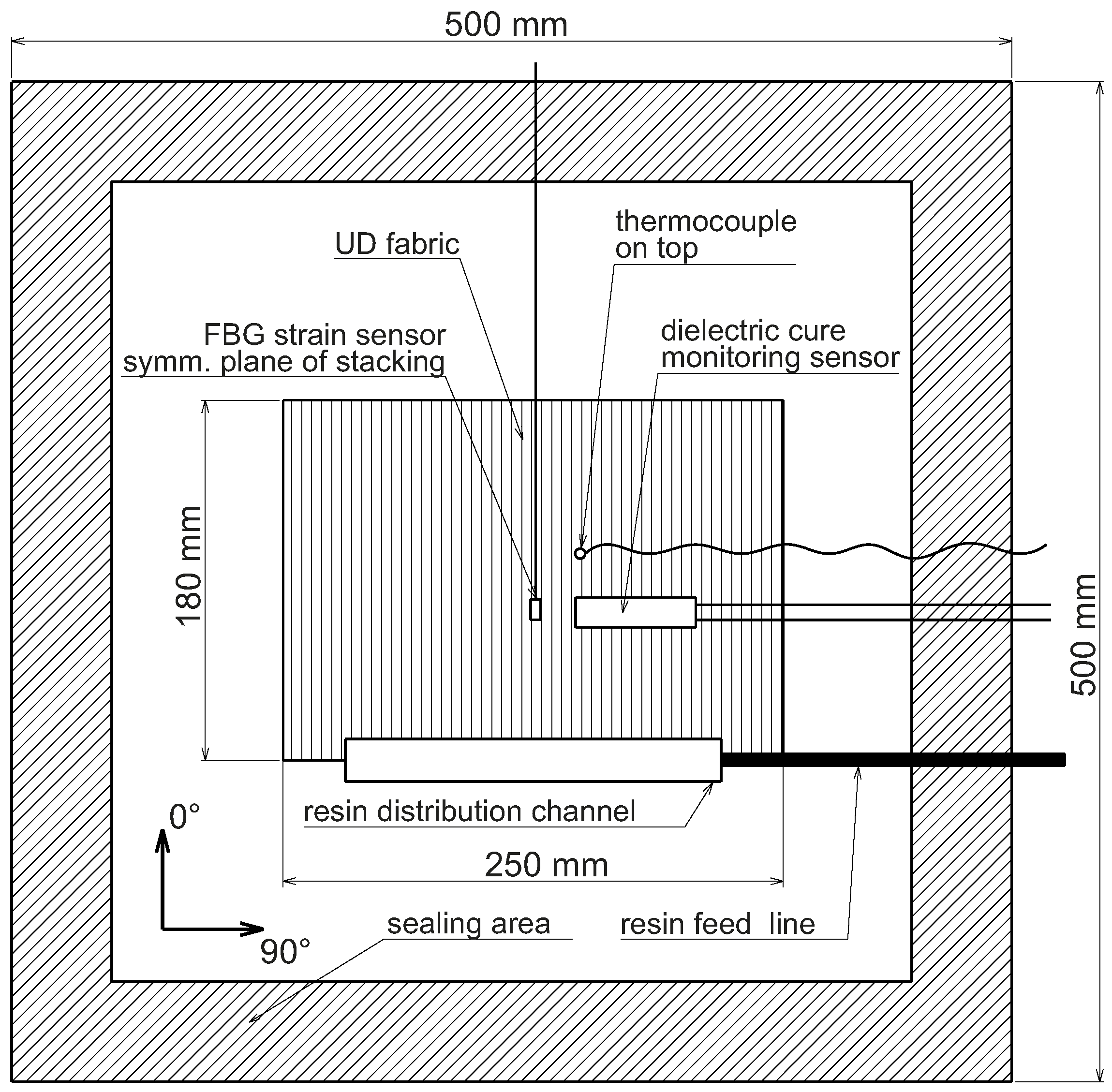
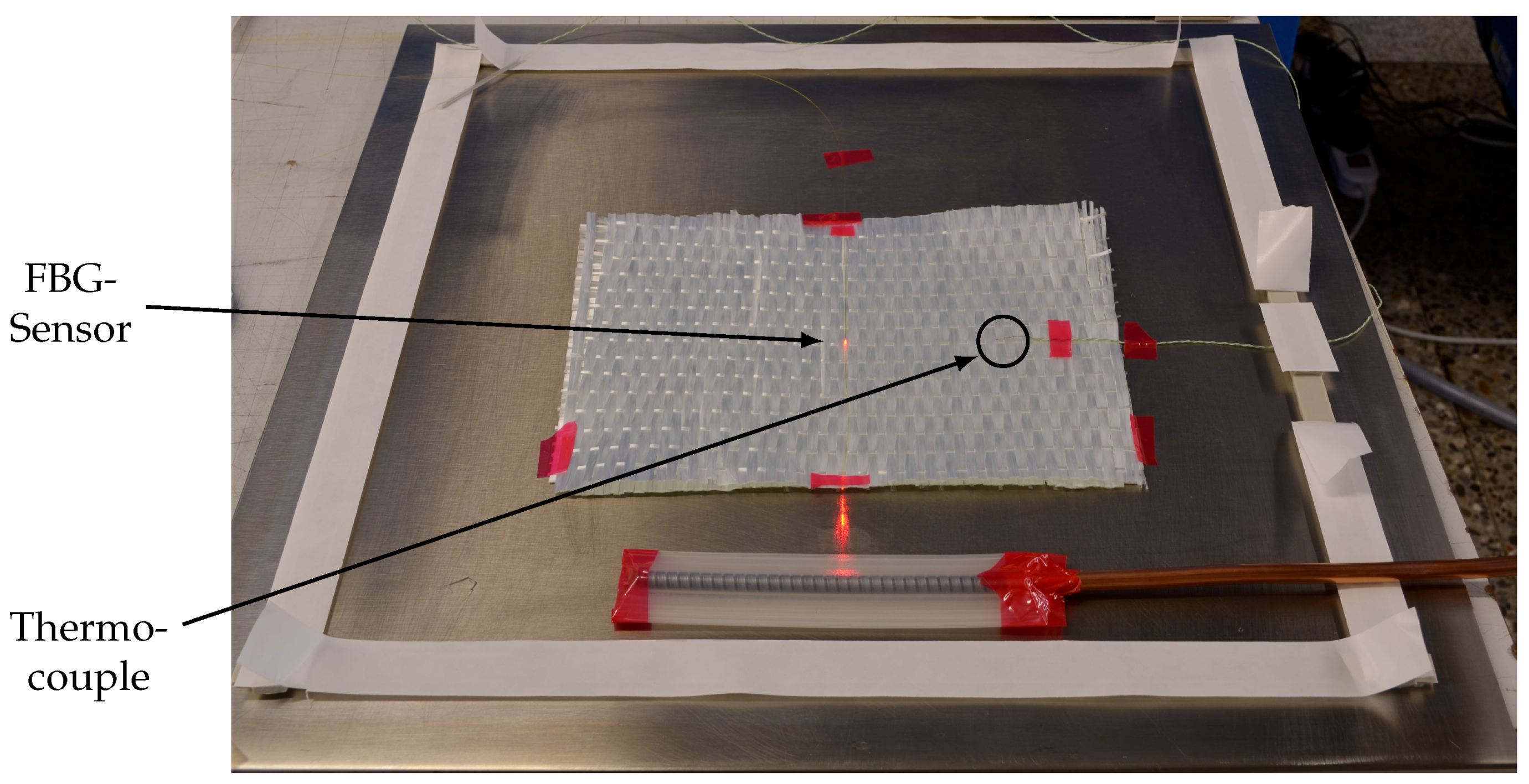
3. Experimental Set-Up

3.1. Applied Manufacturing Process

For the investigations, three cross-ply panels with the dimensions 500 mm × 500 mm (Figure 1) are manufactured. The plies are stacked according to stacking sequence in Table 1. The fiber Bragg sensor is embedded in the plane of symmetry. Figure 2 illustrates the position of the fiber Bragg sensor. The specification of the used fiber Bragg sensor is given in Section 3.2. In addition, a type K thermocouple sensor is placed close to the fiber Bragg sensor for subsequent temperature compensation and in order to measure the laminate temperature. The cure sensors are placed on the top of the last ply and are covered by a peel ply. The specification of the used cure sensors is given in Section 3.3.
The panels are manufactured consecutively in a two stage curing process: an initial curing step and a post-curing step. A flat metal plate with a thickness of 5 mm made from stainless steel 1.4301 [21] as shown in Figure 2 is used as tooling. Zyvax Departure release agent [22] is applied to the tool surface according to the specifications in the technical data sheet. At the beginning, the tooling with the dry fibers, the sensors and the vacuum bagging on top is placed in a laboratory furnace and preheated to 63 ° C . After the laminate temperature reaches 60 ° C , the single line infusion is started at an applied absolute pressure of 0.5 mbar. The resin container is placed outside of the furnace at ambient pressure and room temperature. After 30 min , the fiber layup is completely infiltrated and the infusion hose is disconnected. The initial curing step is proceeded for 60 min at 60 ° C . In a next step, the furnace is switched off and the panel is cooled down to room temperature by natural convection. The data acquisition is proceeded. In a post-curing step, the panel is heated up with a heating rate of 2 K / min to 150 ° C , and is cured for 150 min according to the manufacturer’s recommended cure cycle (MRCC) [12]. The panel is finally cooled down to room temperature by natural convection. The applied cure cycle is depicted in Figure 3.
The described cure cycle is used for two panels. Based on the two tests, a drop in the strain signal during the heating phase to the post-curing temperature is observed. The drop is caused by either a detachment of the laminate from the mould or by a sliding of the fiber Bragg due to material weakening close to the glass transition temperature. For further investigations and to assign a mechanism a third plate is manufactured at a lower heating rate ( 0.5 ° C / min ) and at a lower post-curing temperature (130 ° C ) to prevent a material change from the glassy state to the rubbery state. The applied parameters were determined based on DSC measurements in advance.
The dielectric cure monitoring system as well as the strain measurement system are stand-alone devices. Both have additional temperature measurement channels using thermocouples. Temperature data as well as a global time stamp are used to ensure synchronism between both data acquisition systems.

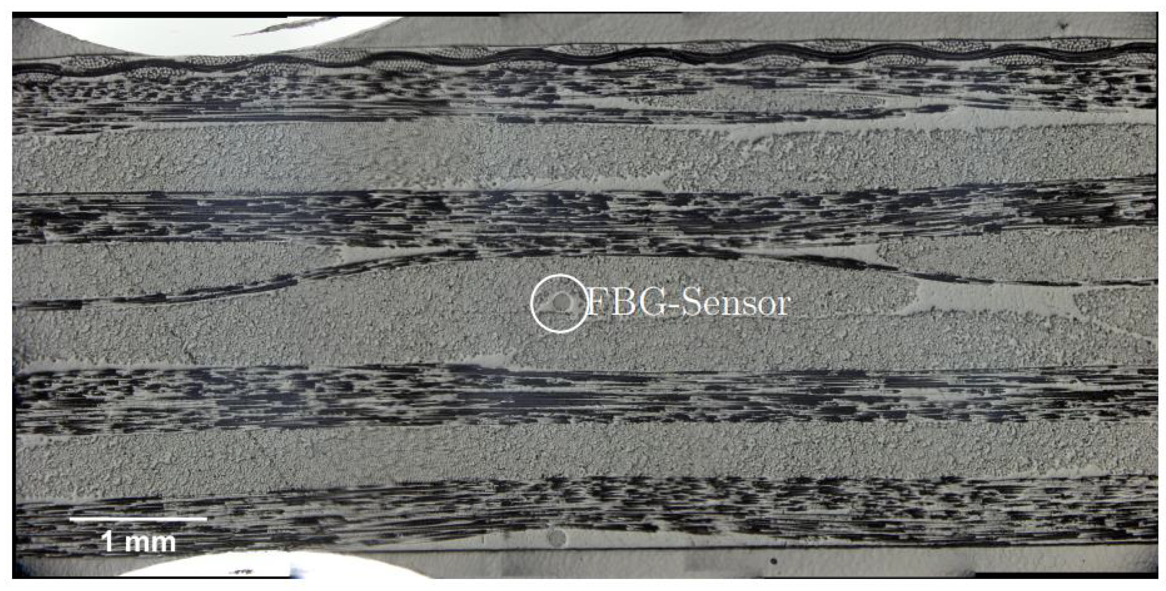
3.2. Fiber Bragg Grating Sensors

A FBG sensor describes an optical single mode fiber (Ø 0.125 mm), which contains the so-called Bragg grating in the fiber core (Ø 0.007 mm). The Bragg grating is a periodical modulation of the refractive index. The gratings of the used sensors have a spread of 2.5 mm. When the fiber is strained by ε or submitted to a temperature change Δ T , a shift of the Bragg wavelength Δ λ b λ b (back reflected wavelength) occurs due to a change of the period of the grating and the refractive index [23]. In the case of an embedded sensor, the expansion of the optical fiber corresponds to the expansion of the bedding material. However, when a FBG is used to measure processing strains in an FRP laminate, the thermo-optic effect of the temperature on the sensor signal needs to be compensated. The calculation of the total strain ε transferred to the optical fiber during the process, including thermal expansion during the heating stages, cure shrinkage and the cooling thermal shrinkage, is conducted by the following equation [24].
ε = Δ λ b λ b C T Δ T C S
The coefficient C S corresponds to a geometrical change of the grating, and is given as a constant of 0.78 [23]. The thermo-optic factor C T , which corresponds to thermal induced change of the refractive index of the grating, was determined with 6.2 ppm/K in previous investigations [24]. The determined sensor parameters and the measuring method were successfully validated in various investigations and comparative measurements with strain gauge sensors and TMA tests [25].
For the experimental investigations, a polyimide coated silica glass FBG sensor is embedded in the described GFRP laminates. The optical fibers are longitudinally (0°) placed between the centre layers as shown in Figure 2. The Bragg grating (sensor) is located in the centre of the samples. The outside diameter of the optical fiber, including the polyimide coating, is ~150 μ m . The variation of the reflected light wavelength by the FBG during curing in an oven is monitored using an optical sensing interrogator (MIOPAS SPK155), whose wavelength range is 1520 nm to 1560 nm. The interrogator operates as light source and spectrometer. The exact wavelength shift can be determined by a peak detection of the reflected wavelength band. Both, temperature and wavelength change are measured with a sampling rate of 1 Hz. The fiber optical measurement method records a processing strain profile during the complete process by using Equation (1). The residual strains, which are used for calculation of the residual stresses, are recorded at room temperature after finishing manufacturing. Using the classical laminate theory (CLT) approach, an apparent thermal load can be calculated from the measured strain ε and the stiffness matrix A:
n T = A · ε
Due to the equal stiffness, as well as the ply thickness in x- and y-directions and the cross-ply-stacking, the strains are assumed to be equal in both directions. Furthermore, the temperature and strain are considered constant over the thickness of the laminate. With the help of the thermal load n T and the thermal expansion coefficient of the laminate α T , a temperature change Δ T can be calculated from
n T = A · α T · Δ T
Thus, the residual stresses in the individual layers can be determined by using the CLT approach with the thermal expansion coefficient of each layer by the following equation
σ R k = Q k · { ε } α T · Δ T k ,
where Q k represents the stiffness matrix of the particular layer. This equation is used later to calculate the residual stresses based on the measured strain.

3.3. Dielectric Cure Monitoring

The dielectric cure monitoring system PDE-1 provided by Gel Instrumente [26] is used. This system allows the use of flat interdigital sensors that can stay on or inside the specimen even after it was demoulded. This means one can reconnect the sensors again to monitor the cross-linking during post-cure outside the mould. The measured conductivity describes the mobility of the charge carriers inside the matrix and their ability to align. Ongoing cross-linking between resin and curing agent leads to an increased viscosity and therefore to a decreased mobility of the charge carriers. As a result the conductivity declines during the curing process. At the moment the glass transition temperature exceeds the current curing temperature the matrix loses its viscoelastic behaviour and dipoles and ions are not able to align or move any more. This means conductivity is at the lowest level. As the dielectric cure monitoring system works with the orientation and the mobility of the charge carriers it enables also a detection of the material weakening during post cure.

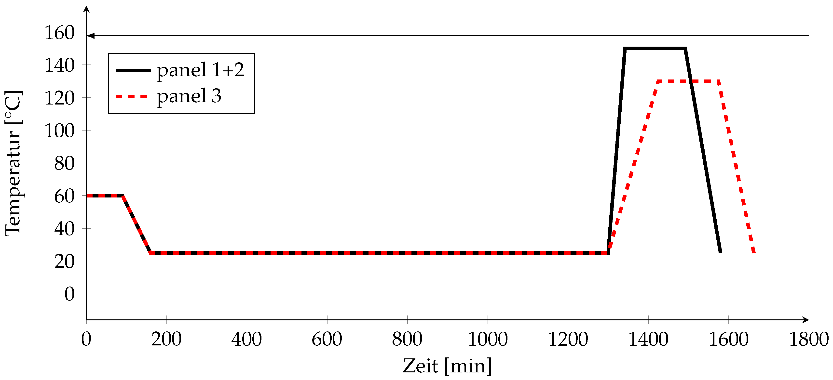
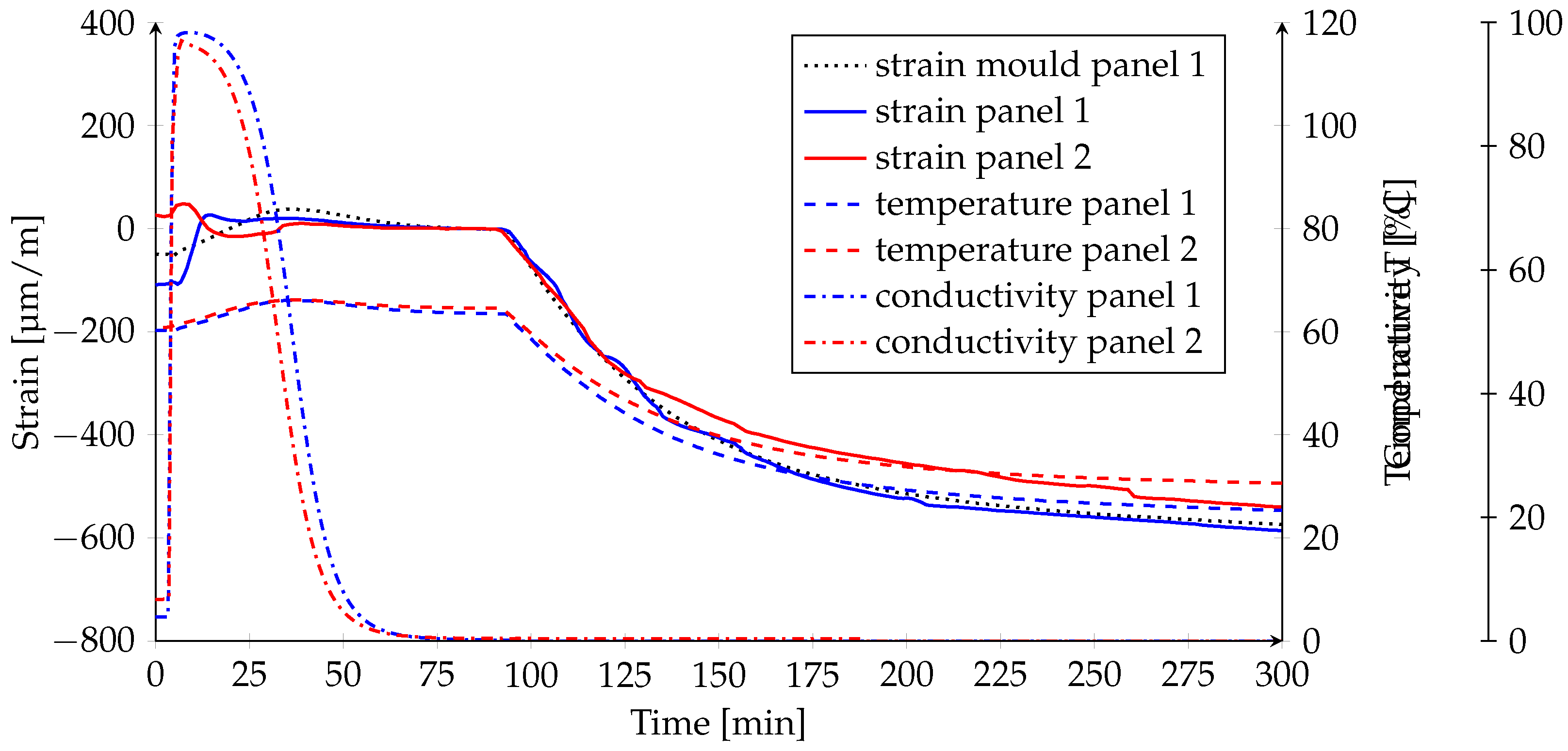
4. Experimental Results

As mentioned in the previous section, a deviating cure cycle for the post-curing step for panel 3 is used. Therefore, the results of the first two panels are analysed at first and the results of panel 3 separately.

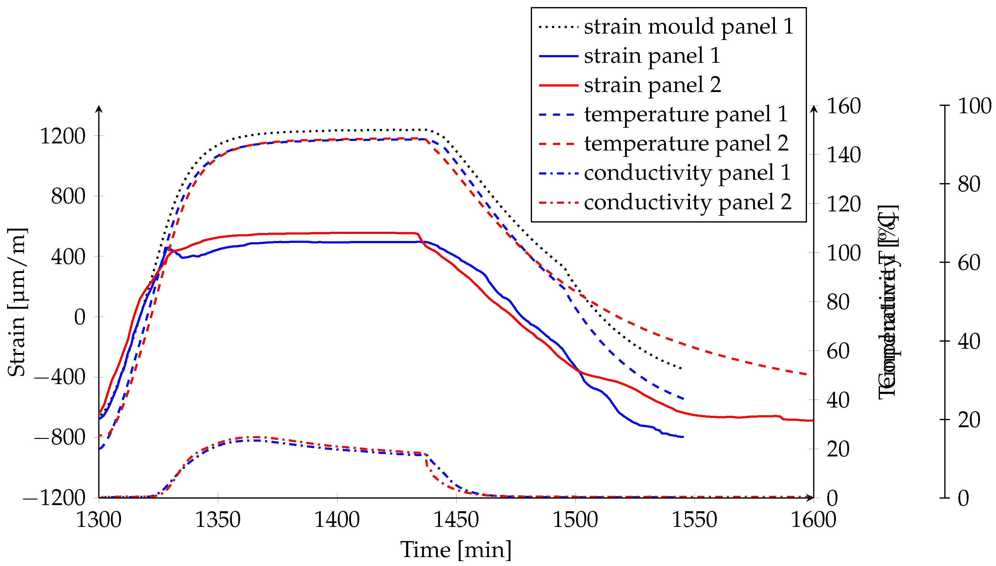
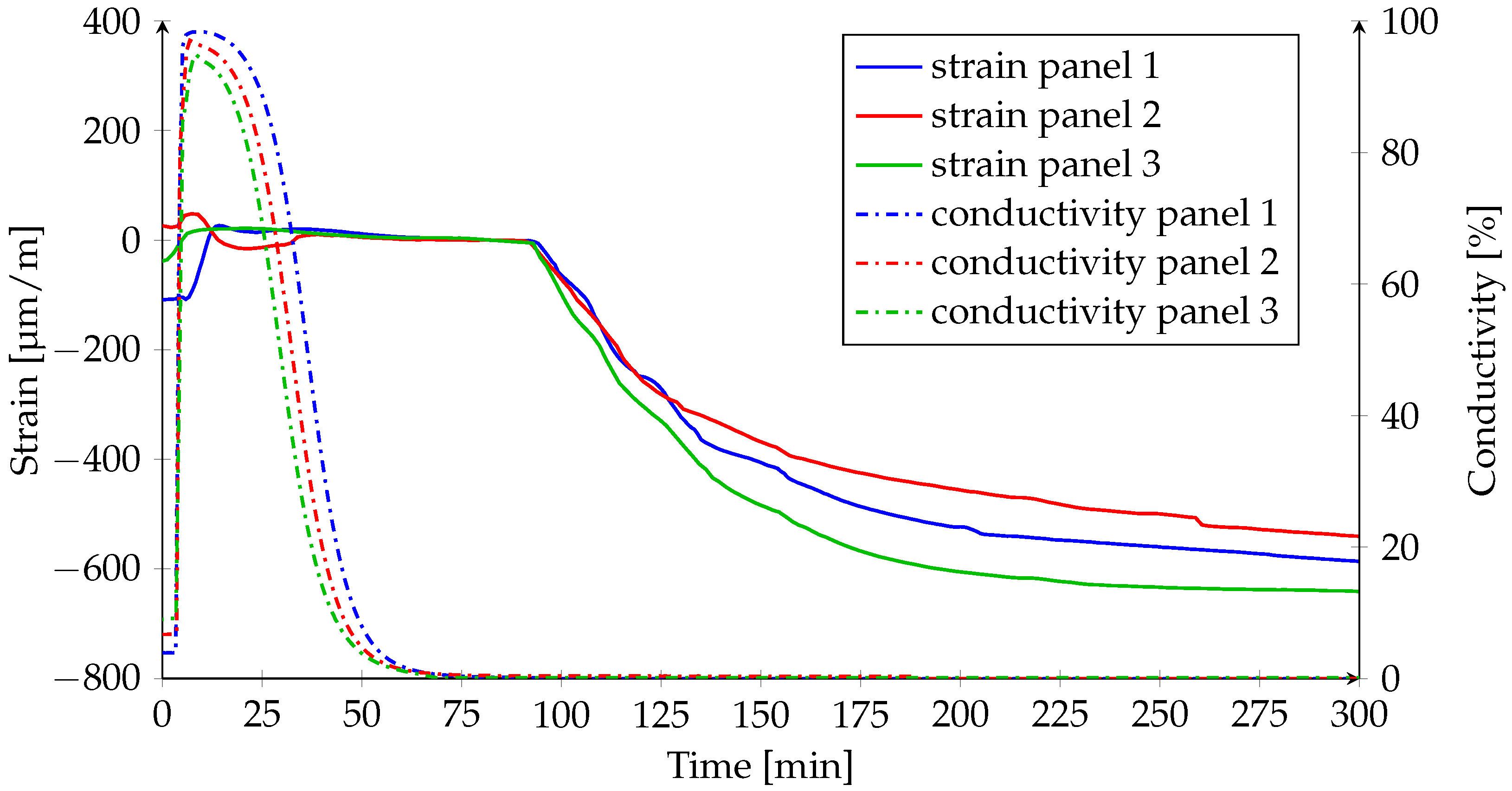
4.1. Results Panel 1 and Panel 2

Figure 4 and Figure 5 show the measured temperatures, strains and conductivities for panels 1 and 2. For a better overview, the data is split into the initial curing step (Figure 4) and the post-curing step (Figure 5).
Referring to the initial curing step a slight temperature increase of about 5 ° C due to exothermic reactions occurs in the laminate after ≈ 40 min.
For both panels, the resin wets the dielectric sensor after ≈ 4 min and the conductivity increases sharply to 98%. Afterwards, the conductivity starts to drop; this is caused by progressing cross-linking and associated limiting mobility of the ions in the resin. After ≈ 89 min the conductivity is close to zero and no changes in the slope of the signal can be observed. This means that the resin is in a solid state after ≈ 89 min . For panel 2 the conductivity decreases earlier. For verification of these results, a DSC measurement as well as a rheometer measurement with the same cure cycle is performed. For determination of the point of gelation the gap change during isothermal curing according to [27] is measured in the rheometer. The neat resin specimen is cured at a temperature of 62 ° C . The point in time when the gap decreases is taken as gel time. Therewith, a gel time of 82 min is determined. The isothermal DSC measurement at 62 ° C has shown a glass transition time of 86 min . This means that the material changes after 82 min from a liquid to a rubbery phase and after further 4 min to the glassy phase. That is in accordance with the conductivity measurement.
Besides the measured strains, the theoretical strain of the steel mould is depicted. The thermal strain of the mould is calculated based on the measured laminate temperature for panel 1 and the CTE of 16 ppm/ K [21]. All strains are shifted along the y-axis so that the strains are zero at the gel point (t = 82 min ). The gel point is chosen because process-induced stresses and strains can arise and be transferred from this point.
At the beginning of the process, the measured strains increase due to the infusion process, causing interaction between the sensor and the flow of the resin material, as well as due to pressure and temperature changes. The increase starts after the raise of the conductivity signal, which means that the dielectric sensor at the upper outside is wetted first and then the FBG sensor in the middle of the panel. Accordingly, the panel is infiltrated from the outside to the center. After ≈ 45 min , a small drop in the strain signals can be observed which is mainly driven by the temperature reduction and a possible chemical shrinkage. However, the drop is very small because of the fiber-dominated direction. Therefore, there are no detectable shrinkage effects which might influence the residual stress state. In the subsequent cooling phase to room temperature the strains decrease after 300 min to 586 μ m / m for panel 1 and to 540 μ m / m for panel due to thermal contraction. Note that the temperature of panel 2 was with 30 ° C slightly higher in comparison to 25 ° C for panel 1 which is the cause for the difference. At the beginning of the post-curing after 1300 min and at room temperature, the strain of panel 1 decreases to 676 μ m / m . The strain of panel 2 is with 636 μ m / m very similar to panel 1. This demonstrates the reproducibility of the measurement results. Furthermore, it can be seen in Figure 4 that the mechanical strain follows the strain of the mould. Based on this, it is assumed that the mould and the panel are tightly connected in this phase.
During the heating phase to the post-curing temperature in Figure 5, the strains of the panels and the steel mould increase identically due to thermal expansion. At ≈ 80 ° C , the gradient decreases. This temperature corresponds to the glass transition temperature of the panels after the initial curing. This was analysed by additional DSC measurements. Simultaneously, the conductivity rises as well. This can be interpreted as an indicator that the material is softening due to the transition from glassy to a rubbery material state. At ≈ 100 ° C , the mechanical strains of the panels drop. It is assumed that the panels detach from the mould and forced strains from the interaction between tool and part are relaxed. Subsequently, the strains increase slightly due to thermal expansion. However, the strain gradient is lower than before due to fiber-dominated material properties in the rubbery material phase. During the following isothermal phase, the mechanical strains are almost constant at 495 μ m / m for panel 1 and 547 μ m / m for panel 2, respectively. No shrinkage or relaxation effects are observed. Within the dwell time the conductivity decreases smoothly due to progressive cross-linking. However, it does not drop to zero so that it is expected that the material is in the rubbery material phase.
At the end of the subsequent cooling phase, the strain for panel 1 decreases to approx. 800 μ m / m at a temperature of 40 ° C . The strain of panel 2 is with 795 μ m / m identical. The data acquisition for panel 1 could only take place up to this time. At room temperature the strain of panel 2 finally decreases to 1053 μ m / m . This represents a maximum strain difference between curing and room temperature of 0.16%. The measured strains correlate well with the results from Balvers [10]. The conspicuous ondulation of the strain signals is caused by sticking and slipping effects of the panels on the mould. A similar behaviour was documented by Fernlund [28] using strain gauges.
The conductivity decreases with the beginning of the cooling phase and drops to zero after ≈ 1475 min or at a laminate temperature of ≈ 100 ° C . From this point on, the cooling takes place in a glassy material state.

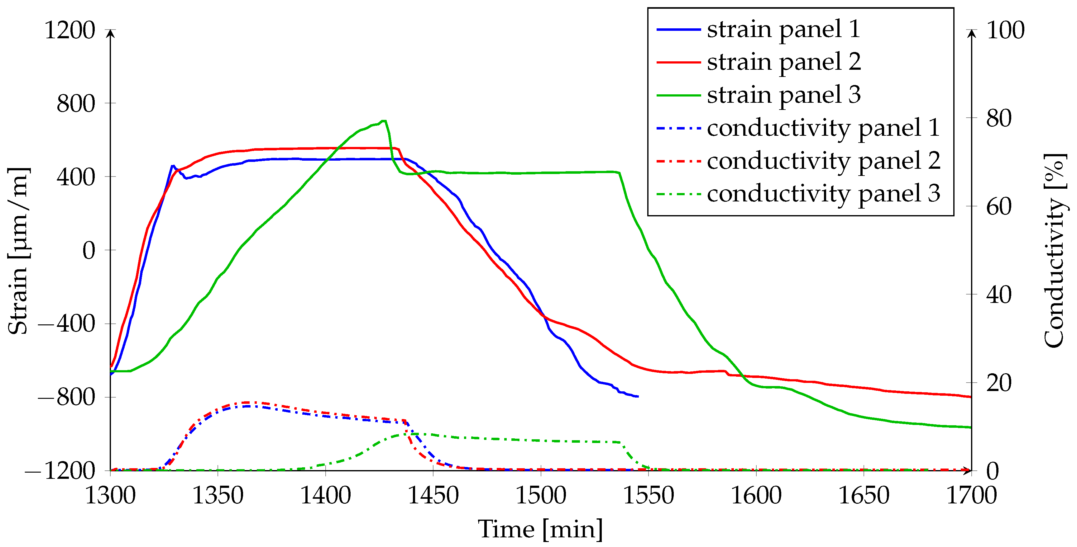
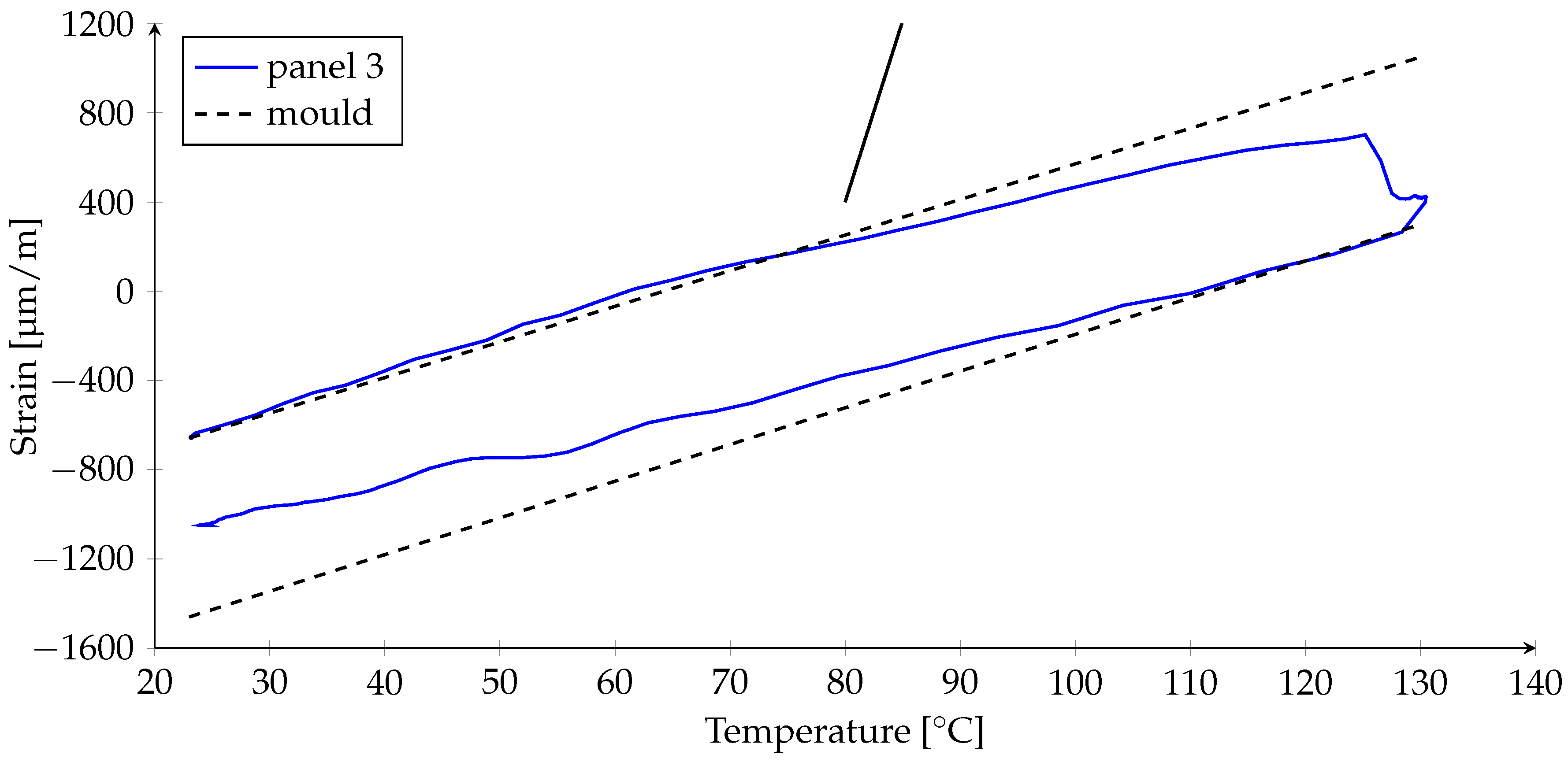
4.2. Results Panel 3

The initial cure for panel 3 is performed according to the previous two panels. Figure 6 shows the measured strain and the conductivity for all three panels.
For the sake of clarity, the particular laminate temperatures are not plotted, but it should be noted that these are not identical, which leads to the slight differences in the strain gradients. The qualitative development of the mechanical strain in the initial cure is identical to the other two panels. At the end of the initial curing process, after 1300 min and at room temperature, a strain of 659 μ m / m is measured. This is similar to panel 1 with 676 μ m / m and panel 2 with 636 μ m / m . Based on this a relative variation of ±3% of the strain signal in maximum is observed. The decrease of the conductivity is slightly earlier compared to the other two panels but the drop to zero at ≈ 80 min is similar. Therewith, all three panels own the same initial curing.
Figure 7 shows the results for the different post-curing steps. For panel 3, a lower heating rate of 0.5 K / min and a lower overall curing temperature of 130 ° C is applied. The modified cycle is used in order to avoid an exceedance of the glass transition temperature during the post-curing. The heating rate is determined based on previous performed DSC measurements. Therewith, it shall be investigated if the drop of the laminate strain is caused by a detachment of the laminate or by a sliding of the fiber Bragg. The modification is also performed to investigate whether a variation of the post-curing process affects the resulting residual strain level.
During the heating phase, the strain increases from −660 μ m / m to 701 μ m / m due to thermal expansion. The higher strain level compared to the first two panels is occurs because the panel is longer connected to the mould, and therewith higher strains a transferred from the mould to the laminate. At a temperature of ≈ 126 ° C the strain drops to 413 μ m / m due to the detachment of the laminate from the steel mould. It is assumed that the laminate can not follow the strain of the mould any more. In the following isothermal curing the strain remains constant.
The conductivity rises at a temperature of 96 ° C , which is higher in comparison to the other two panels (≈ 80 ° C ). This shows that the glass transition temperature is increased due to the slow heating rate and further curing. With increasing temperature the conductivity rises constantly to its maximum value of ≈8% which is less compared to the the first two panels with ≈15%. This shows that the ion mobility is restricted due to the higher degree of cure. Furthermore, it indicates that a weakening from a glassy to a rubbery state does not take place to the same extent in panel 3 as in panel 1 and panel 2. Note that the glass transition is not an absolute value, it is rather a transition zone. As the conductivity is close to zero, it is expected that the material is in a glassy material phase or in the beginning of the glass transition zone but not in the rubbery phase. The drop is therefore a result of the separation of tool and part, and not a result of a sliding of the fiber Bragg due to material weakening or due to shrinkage or relaxation effects of the plastic matrix material. This is also confirmed by Figure 8. During the cooling phase, no change in the strain slope could be observed. Based on that, no material transition is expected so that the cooling is done in the glassy state. The strain is mainly driven by the thermal contraction and decreases finally to 1047 μ m / m at room temperature, which is comparable to panel 2 with 1053 μ m / m . This means that the modified post-curing process results into the same strain level despite of a lower curing temperature and lower heating rate. The maximum strain difference of 413 μ m / m − (− 1047 μ m / m ) = 1460 μ m / m (0.15%) is slightly lower compared to panel 2 with 0.16%, but not significant.
The measurements have shown that the different heating rates during the post cure influence the curing rates and thereby the characteristic points of material transitions. This results in different strain curves and influences the point of detachment between tool and part. However, the residual strain levels after manufacturing at room temperature are independent of the post-curing process. This supports the statement that the time of the connection of the different components (fiber and matrix material) as well as the temperature and the stress state prevailing at this time are decisive for the storage of the residual stresses during the manufacturing process [24,25]. This characteristic point is related to the gelation of the plastic matrix material. After crossing the point of gelation, the in-plane laminate material properties are fiber-dominated. The subsequent strains in the manufacturing process are therefore to be interpreted as almost elastic and reversible.
Regarding the investigation of the tool–part interaction, Figure 8 shows the measured strain in dependency on the temperature of the post-curing step of panel 3. Additionally, the theoretical strain of the mould is plotted. During the heating phase, until 65 ° C , the strain of the laminate follows the strain of the mould. This means that either the tooling or the laminate have the same effective coefficient of thermal expansion or both parts are sticking together. To investigate this, two specimens from the cured plate are cut-off and the coefficient of thermal expansion is determined via thermal mechanical analysis. For the cross laminate, a CTE of multi-part-units = brackets ( 13.73 ± 1.46 ) × 10 6 1/ K was determined. This is in agreement with the CTE of 13.6 × 10 6 1/ K determined based on the fiber Bragg measurement in Figure 8. For the calculation, the cooling phase between 130 ° C and room temperature was analysed. This correlates also with the calculated CTE of 14.9 × 10 6 1/ K using the CLT and the values from Table 2. Therewith, the CTE of the laminate is slightly lower than for the mould with 16 ppm/ K . The coefficients of thermal expansion are close to each other, but not identical. Therefore, it is expected that during the heating phase both plates stick together and the strain of the mould is transferred to the laminate. At a temperature of ≈ 65 ° C , the laminate strain decreases in comparison to the strain of the mould. This temperature is close to the glass transition temperature or the transition zone after the initial curing step. Here, the material begins to soften and the material properties change. As the fiber properties become dominant at the glass transition temperature, the strain decreases because of the lower CTE of the fiber material. At 125 ° C , the strain drops abruptly because of the detachment of the laminate from the mould. The detachment is probably triggered by the increasing differences in the strains between the laminate and the mould as well as the increasing degree of cure. In comparison to the heating, an oscillation in the strain signal can be observed during the cooling. It is assumed that the laminate and the mould interact mechanically and a change of static and dynamic friction occurs. Due to the smaller coefficient of thermal expansion of the laminate, the final strain after cool down is lower compared to the mould. The different strain levels exhibit that the laminate and the mould were detached during the cooling.
For verification of the local FBG-sensor position and orientation, a cross-section of the GFRP laminate was created. As depicted in Figure 9, the sensor is well embedded in fiber direction. However, resin-rich areas are formed around the sensor. These areas can influence the measured signal in a way, so that not the pure strain in fiber direction is measured.

5. Process Simulation

Within this section, the used FE-Model, the applied boundary conditions and the simulation results of panel 3 are presented. For validation, the measured process strains are correlated with the calculated strains.

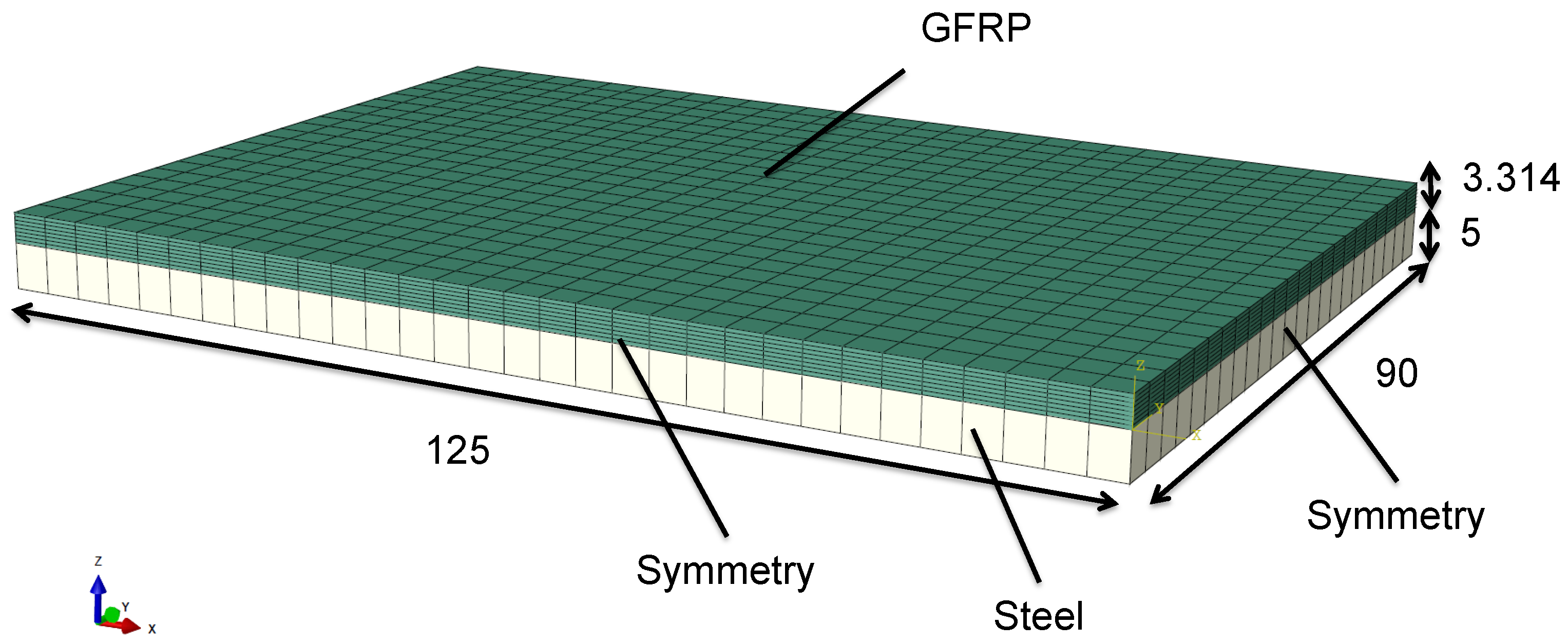
5.1. FE-Model and Boundary Conditions

To reduce the modelling effort and the calculation time, symmetry conditions are used and only a quarter model of panel 3 is created (Figure 10). Each layer of the laminate is meshed with one homogeneous solid element (C3D8R) in thickness direction. The fiber orientations are assigned according to the stacking in Table 1.
The temperature measured close to the fiber Bragg is applied as fixed temperature to all FE nodes as simplified thermal boundary condition. The curing process is divided into four calculation steps. In the beginning the material is in a liquid material phase. To avoid the transmission of shear stresses into the laminate by the expanding mould, a frictionless contact condition is defined between mould and laminate (step 1). After crossing the gel point, it is assumed that the mould and the laminate are bonded together (step 2). A rough contact boundary condition is employed to tie the two parts together and is sustained for the subsequent cool down and dwell period. During the second heating a detachment of the laminate from the mould was observed in the FBG-signal. For consideration in the simulation, the rough contact is deactivated and isostatic displacement boundary conditions are applied to the laminate to avoid free body motions (step 3). For a better approximation of the mechanical boundary conditions, a frictionless contact may be applied between the laminate and the mould. However, to reduce the simulation time, the described procedure was utilised. Due to the plane plate, no significant differences are expected in comparison to the contact boundary condition. The post-curing and cool down process is continued with the described boundary conditions (step 4).

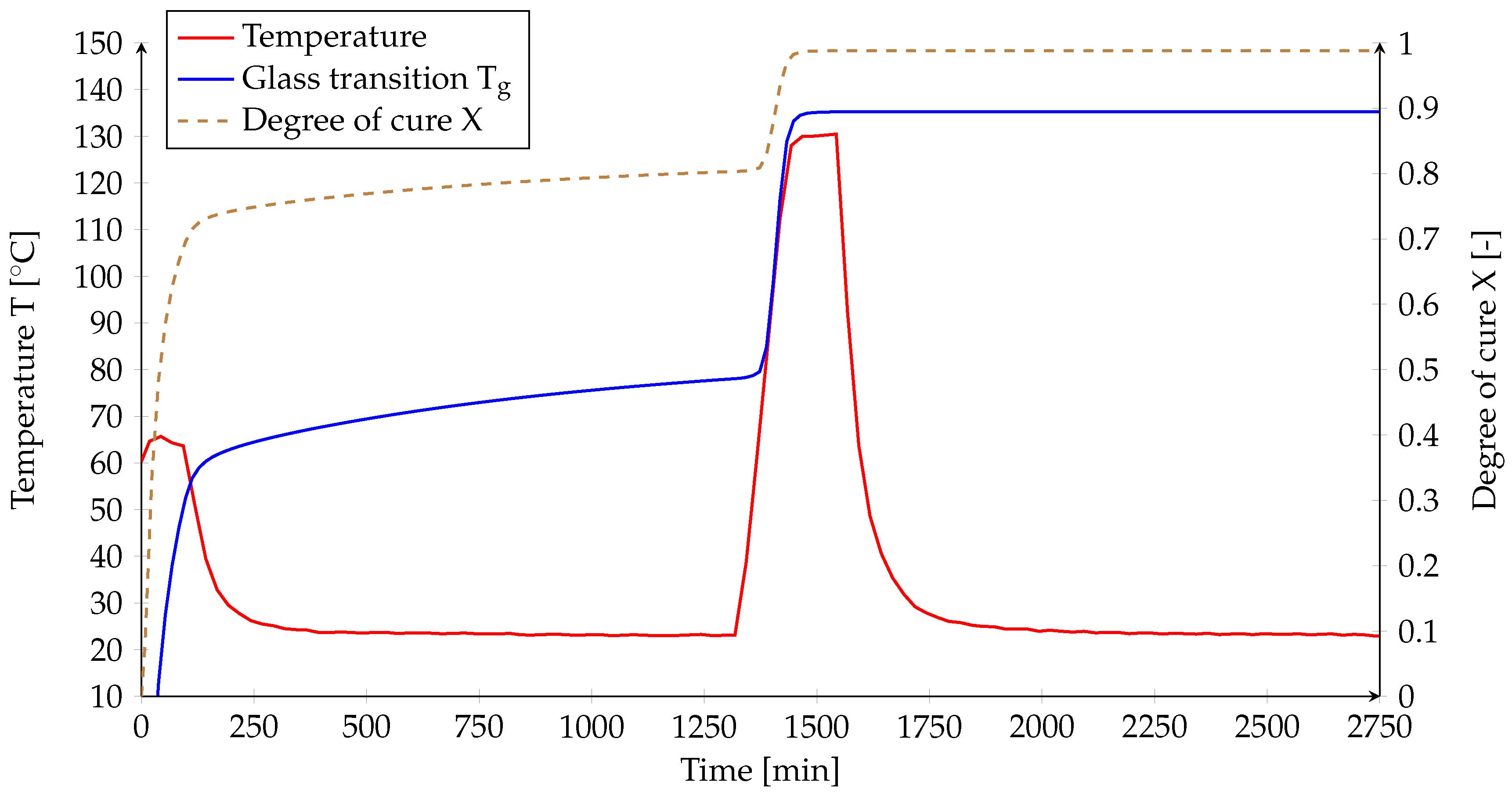
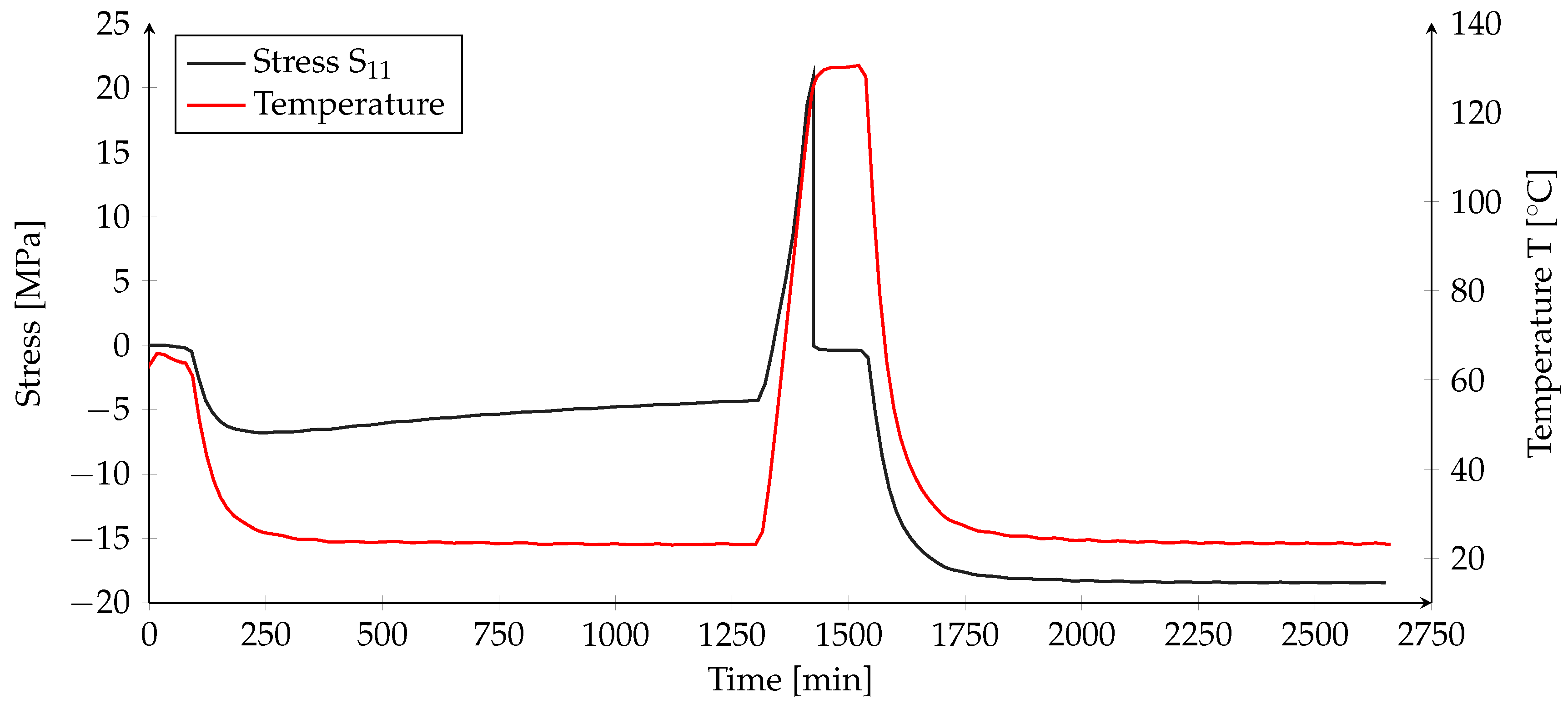
5.2. Simulation Results

Figure 11 shows the development of the degree of cure (brown) and the glass transition temperature (blue) in dependency on the measured laminate temperature (red).
For evaluation a node close to the local position of the FBG-sensor is used (see red point in Figure 11). After the first dwell phase (t = 90 ), a degree of cure of 68% and a glass transition temperature of T g 50 ° C is calculated. For validation of the calculated glass transition temperature, a further fourth panel without sensors is manufactured with the same conditions. During manufacturing small specimens for DSC analysis are extracted after 90 min and 1300 min before post-cure. The measured glass transition temperature correlates with 50 ° C with the predicted value. For the end of the dwell phase, at room temperature, a glass transition temperature of 78 ° C is predicted. This correlates well with conducted isothermal DSC measurements at a curing temperature of T = 60 ° C . For these, glass transition temperatures between 75 ° C and 80 ° C are obtained. In contrast, the measured glass transition temperature of the laminate after 1300 min is 64 ° C . This means that the trend of a rising glass transition temperature is well approximated by the model, but the glass transition temperature is overestimated by the model. The deviation of the predicted value from the measured values can have several causes. For the determination of the reaction kinetic model no isothermal measurements for 60 ° C are utilised. This can lead to deviations in the prediction of the degree of cure and the corresponding glass transition temperature. The measurements are conducted for the neat resin. The coating of the fiber or the binder material may influence the curing behaviour. In the simulation, a degree of cure of zero is assumed as initial state for the entire model. The mixing of resin and hardener, degassing and preparation of injection takes ≈ 45 min. In this time, the degree of cure may increase slowly and can effect the degree of cure. This is not considered in the simulation.
Next, the post-curing phase is analysed. During the heating to the cure temperature of 130 ° C , the glass transition temperature is always above laminate temperature. This was also approved by DSC analysis. In comparison, for panels 1 and 2, the laminate temperature is above the glass transition temperature during the heating phase. Within the second dwell phase the glass transition temperature arises to 135 ° C . The measured glass transition temperature after the post-curing step was 132 ° C , which means a deviation of ≈2.3% from the simulation. The calculated value is in the measured range for the glass transition temperature.

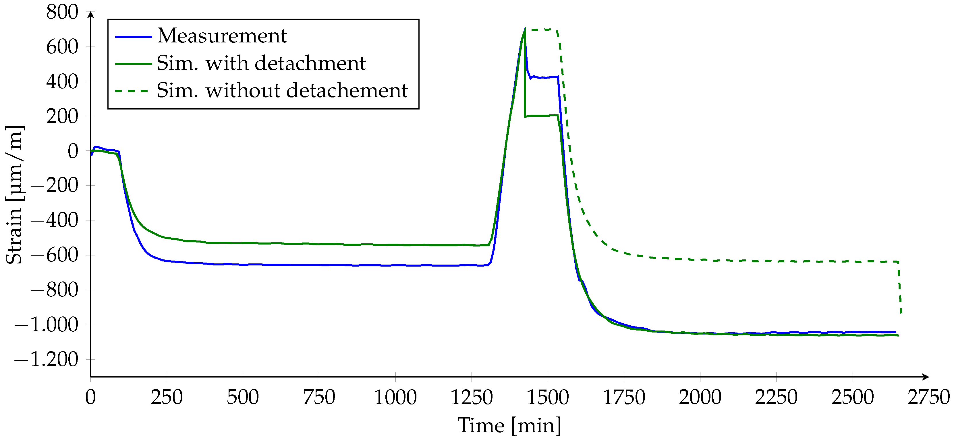
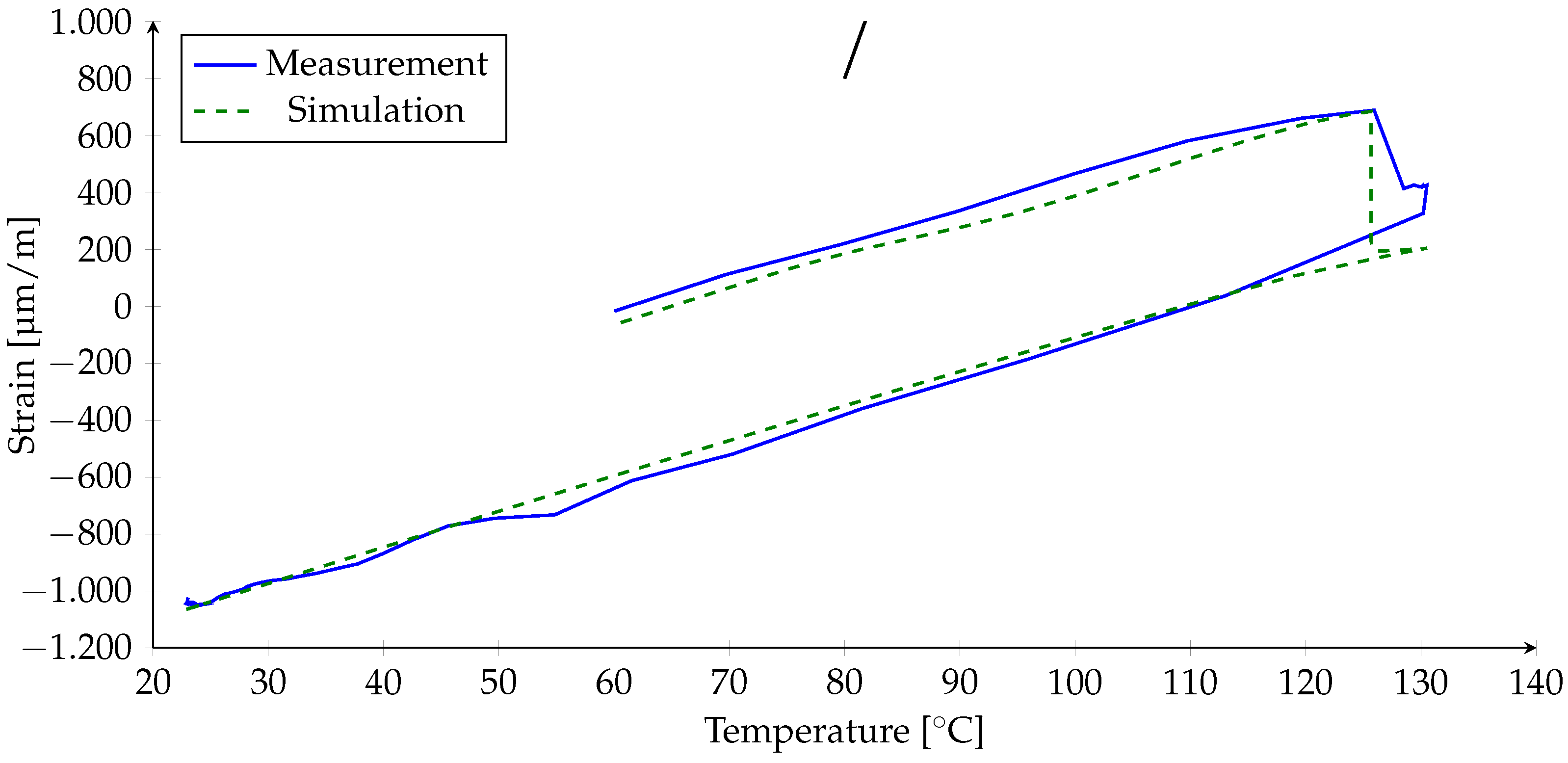
Comparison of the Strains

For validation of the simulation, the simulated strain is depicted for two simulation cases in comparison to the measured strain of panel 3 in Figure 12. In the first case, the process strains are predicted for the case that the detachment occurs at the measured time of separation. In the second case, the detachment is modelled at the end of the process. In the case without detachment, the rough contact condition is active until the end of the process.
At first, the simulation with the detachment at the measured time point of separation is analysed. During the first dwell phase, the measured and simulated strain is almost identical. In both signals, a small drop of the strains due to chemical shrinkage is observed. After cool-down to room temperature, the measured strain of 660 μ m / m is higher in comparison to the simulated strain of 545 μ m / m , which is a relative deviation of 17%.
In the subsequent heating phase, both strains are identical. After approximately half of the heating phase, a slight decrease in the slope of both signals is observed. According to Figure 8, the temperature is close to the glass transition temperature and the fiber properties become dominant. Additionally, the mechanical as well as the chemical strains are superposed, resulting in a decreased slope in the strain. Both strains reach simultaneously the maximum tensile strain of 770 μ m / m . Afterwards, the strain drops due to the detachment of the laminate from the mould. In the simulation, the strain drops by 500 μ m / m to 200 μ m / m , whereas the measured strain drop only by 280 μ m / m to 420 μ m / m . The time of the detachment in the simulation is modelled based on the measurements. Afterwards, both strain curves are constant due to the constant temperature and no further cross-linking reactions. Both strain curves are identical during the cooling phase. The final simulated strain at room temperature is 1060 μ m / m . The relative deviation to the measured strain of 1040 μ m / m is with 1.9% very small, so that a good correlation is achieved.
To show that the drop in the strain signal is caused by the detachment of the laminate from the mould, the dashed line in Figure 12 shows the simulated strain for the detachment applied at the end of the process. The strain signal is identical to the first case due to the same boundary conditions. During the second dwell phase, the strain signal is constant at 770 μ m / m . In the subsequent cooling phase, the strain of the mould is transferred to the laminate and the qualitative trend deviates from the measured strain. The obtained strain at the end of the process is with 630 μ m / m (before detachment) significantly smaller compared to the first case. This comparison shows that a detachment must have taken place. In a last calculation step the demoulding is simulated. The rough contact condition is deactivated and the strain drops to 934 μ m / m , which is smaller in comparison to the first case.
The simulation with the detachment at the moment of separation shows a good correlation with the optical strain measurements. Thus, it is assumed that the applied modelling strategy in combination with the viscoelastic material model is capable to predict the process strains. Furthermore, the calculation without the detachment shows that the mechanical boundary conditions have a significant influence on the prediction of the process strains. In addition, it could be observed that the laminate and the mould are bonded in the early process (low degree of cure) and a detachment is taking place during the process (increased degree of cure). This tool–part interaction needs to be considered in the process simulation. As the conditions for the detachment are actually unknown, it is essential for the correct prediction of process strains to conduct further experimental investigation regarding the tool–part interaction and the detachment conditions.
Figure 13 shows, in comparison, the strains in dependency on the temperature for the post-curing step. During the heating phase, the measured and simulated strains have the same increase. The small offset results from the different strain levels after the initial curing step. After a temperature of 125 ° C is reached both signals drop due to the detachment, whereby the drop of the simulated strain is higher. During the temperature increase to 130 ° C , the strains are constant. In the cooling phase both strains are almost identical. At this point it is to be mentioned that the measurement is conducted in fiber-dominated direction, where only minor relaxation effects occur.
Finally, Figure 14 shows the stress development in fiber direction during the entire curing process. After the first dwell phase and cool down to room temperature, a compression stress of 7 MPa is calculated. The stress relaxes to 4 MPa until the post-curing step begins. During the heating to the post cure temperature, the stress increases to ≈ 21 MPa because of thermal expansion. After the detachment at 130 ° C the stress drops to 1 and relaxes to zero. In the cooling phase, compression stress arises because of a thermal contraction. After cool down to room temperature the residual stress in fiber direction is 18.5 MPa.
To verify the calculated stress the residual stress is calculated by the classical laminate theory and based on the measured strain at the end of the process. With the measured strain of 1044 μ m / m , and under application of Equation (3), a temperature difference of 70 K is calculated. The calculated residual stress using Equation (4) is 19.3 MPa, which correlates very well with the numerical value of 18.5 MPa. Therewith, a good match of the residual stress could be achieved. The used material parameters are summarised in Table 2. The values are obtained by static tension tests according to [29] and thermal mechanical analysis [13,19].

6. Conclusions and Outlook

The main objectives of the present work are to check the usability of different sensors types to monitor the manufacturing process of fiber-reinforced plastics, to investigate tool–part interactions and to validate the applied process simulation method. For process monitoring, the process strains of three GFRP cross-ply panels were measured by means of fiber Bragg grating sensors. Additionally, dielectric sensors were applied to detect the material phases such as the liquid, rubbery and glassy material state. Parallel to the experimental investigations a process simulation for panel 3 was performed.
Both sensors—fiber Bragg grating sensors and dielectric sensors—could be successfully applied for process monitoring. The sensors enable the measurement of the process strains of the entire process, and the time point of the detachment of the laminate from the tooling could be determined. Furthermore, the amount of residual stresses ( 19.5 MPa) could be calculated based on the measured strains. The dielectric sensors could be successfully used to identify the resin arrival and the material phase changes. The time point of the material changes were in agreement with performed rheometer and DSC measurements. The strain and conductivity measurements during the post cure of the different panels have shown a significant influence of different heating rates on the resulting strain curves, the tool part interaction and the material transition phases. There is a clear correlation between material transitions, the conductivity as well as a change in the strain slope. However, the final residual strain levels were independent of the different post-curing cycles.
The measured process strains could be represented qualitatively very well by the applied process simulation. After the first dwell phase, there is a maximum deviation of 17%, and at the end of the process, a maximum deviation of 2% was determined. A very good correlation could be observed between the residual stress calculated by the process simulation and the residual stress calculated via the CLT and the measured process strains. The difference was 4% in maximum. The simulation of the moment of the detachment of the laminate from the tooling was modelled based on the measurements. As the specific conditions for the detachment are unknown and in order to simulate the detachment based on boundary conditions, further experimental investigations with respect to the tool–part interactions and the corresponding conditions during the detachment are required. The comparison of the simulated glass transition temperature to DSC measurements shows qualitative and quantitative a very good agreement for different degrees of cure. This confirms, that the reaction kinetics can be approximated sufficiently.
In future, the efficiency in process development can be improved by a sensor support process simulation. By using only few sensors the process simulation can be calibrated, f.i. in terms of optimised boundary conditions. Exemplary, the fiber Bragg grating sensors can be used to identify the interlaminar and tool–part interactions, and thereby determine the material transition phases with its impact on the thermo-mechanical material characteristics as well as the detachment of the laminate from the tooling. The calibrated process simulation enables an enhanced quality management, as all results can be provided for the entire structure and not only for local sensor positions. Based on this, holistic process and component optimisation can be performed in order to decrease process times and increase the component quality before manufacturing. The direct coupling of sensor data and simulation during manufacturing is the basis for a digital twin. In an additional curing process section, dielectric cure monitoring can be used to identify the softening of the laminate in order to adjust the geometry of the part with an adaptive tooling.

Author Contributions

The individual contributions of the authors are: Conceptualisation, R.H., R.P. and J.S.; Methodology, R.H., R.P. and J.S.; Software, R.H.; Validation, R.H., R.P. and J.S.; Formal Analysis, R.H., R.P. and J.S.; Resources, R.H., R.P. and J.S.; Data Curation, R.H., R.P. and J.S.; Writing—Original Draft Preparation, R.H.; Writing—Review & Editing, R.P. and J.S.; Visualisation, R.H.; Supervision, R.H.; Project Administration; R.H., R.P. and J.S.; Funding Acquisition, R.P. and R.H. The manufacturing of the plates as well as the dielectric measurements were conducted by J.S. The installation and analysis of the optical strain measurements are conducted by R.P. The process simulation and correlation with the measurements were conducted by R.H. All authors have read and agreed to the published version of the manuscript.

Funding

The research is supported by the German Research Foundation (DFG) as part of the priority program 1712: Intrinsic hybrid composites for lightweight structures—basics of manufacturing, characterization and design and the research project ECOMISE founded by the European Commission within the framework FP7 (Funded under: FP7-NMP, Grant agreement ID: 608667).

Acknowledgments

The authors gratefully acknowledge the German Research Foundation (DFG) and the European Commission for the financial support.

Conflicts of Interest

The authors declare no conflicts of interest. The founding sponsors had no role in the design of the study; in the collection, analyses, or interpretation of data; in the writing of the manuscript; or in the decision to publish the results.

Abbreviations

The following abbreviations are used in this manuscript:
CLTClassical laminate theory
CTECoefficient of thermal expansion
DSCDifferential scanning calorimetry
FBGFibre Bragg grating
GFRPGlass fiber-reinforced plastics
MRCCManufacturer recommended cure cycle
PIDProcess-induced deformations
TMAThermomechanical analysis

References

  1. Kaps, R. Kombinierte Prepreg- und Infusionstechnologie für integrale Faserverbundstrukturen. Ph.D. Thesis, Technical University of Braunschweig, Braunschweig, Germany, 2010. [Google Scholar]
  2. Shokrieh, M.; Ghanei Mohammadi, A. The importance of measuring residual stresses in composite materials. In Residual Stresses in Composite Materials; Woodhead Publishing: Cambridge, UK, 2014; pp. 3–14. [Google Scholar] [CrossRef]
  3. Puck, A. Analysis of Failure in Fiber Polymer Laminates-The Theory of Alfred Puck; Springer: Berlin/Heidelberg, Germany, 2008; p. 208. [Google Scholar]
  4. Brauner, C. Analysis of Process-Induced Distortions and Residual Stresses of Composite Structures. Ph.D. Thesis, Faserinstitut Bremen, Bremen, Germany, 2013. [Google Scholar]
  5. Harsch, M. Methoden und Ansätze zur spannungsarmen Vernetzung von Epoxidharzen. Ph.D. Thesis, TU Kaiserslautern, Kaiserslautern, Germany, 2008. [Google Scholar]
  6. Prussak, R.; Stefaniak, D.; Kappel, E.; Hühne, C.; Sinapius, M. Smart cure cycles for fiber metal laminates using embedded fiber Bragg grating sensors. Compos. Struct. 2019, 213, 252–260. [Google Scholar] [CrossRef]
  7. Svanberg, J.M. Predictions of Manufacturing Induced Shape Distortions—High Perfomance Thermoset Composites. Ph.D. Thesis, Lulea University of Technology, Lulea, Sweden, 2002. [Google Scholar]
  8. Oliveira, R.D.; Lavanchy, S.; Chatton, R.; Costantini, D.; Michaud, V.; Salathé, R.; Månson, J.E. Experimental investigation of the effect of the mould thermal expansion on the development of internal stresses during carbon fiber composite processing. Compos. Part A Appl. Sci. Manuf. 2008, 39, 1083–1090. [Google Scholar] [CrossRef]
  9. Nielsen, M.W. Prediction of Process Induced Shape Distortions and Residual Stresses in Large Fibre Reinforced Composite Laminates—With Application to Wind Turbine Blades. Ph.D. Thesis, Technical University of Denmark, DTU, Lyngby, Denmark, 2012. [Google Scholar]
  10. Balvers, J.M. In Situ Strain & Cure Monitoring in Liquid Composite Moulding by Fibre Bragg Grating Sensors. Ph.D. Thesis, TU Delft, Delft, The Netherlands, 2014. [Google Scholar] [CrossRef]
  11. Johnston, A.A. An Integrated Model of the Development of Process-Induced Deformation in Autoclave Processing of Composite Structures. Ph.D. Thesis, University of British Columbia, Vancouver, BC, Canada, 1997. [Google Scholar]
  12. Huntsmann International LCC. Araldite ® LY 564* / Aradur ® 2954 *. Available online: https://www.mouldlife.net/ekmps/shops/mouldlife/resources/Other/araldite-ly564-aradur-2954-eur-e-1-.pdf (accessed on 23 January 2020).
  13. Hein, R. Vorhersage und In-Situ Bewertung fertigungsbedingter Deformationen und Eigenspannungen in Kompositen. Ph.D. Thesis, Technical University of Braunschweig, Braunschweig, Germany, 2019. [Google Scholar]
  14. DIN EN ISO 11357-1-2017-02—Beuth.de. Plastics—Differential scanning calorimetry (DSC)—Part 1: General principles. Available online: https://www.beuth.de/de/norm/din-en-iso-11357-1/264864949 (accessed on 8 November 2019).
  15. Mettler Toledo. Available online: http://www.mt.com/de/de/home.html (accessed on 23 January 2020).
  16. Owens Cornings. SE 1500 Roving Datasheet. Available online: http://www.ocvreinforcements.com/pdf/products/10009978_B_SingleEndRovings_SE1500_ww_11_2012_Rev3.pdf (accessed on 23 January 2020).
  17. Poon, H.; Ahmad, M.F. A material point time integration procedure for anisotropic, thermo rheologically simple, viscoelastic solids. Comput. Mech. 1998, 21, 236–242. [Google Scholar] [CrossRef]
  18. Zocher, M.A.; Groves, S.E.; Allen, D.H. A three-dimensional finite element formulation for thermoviscoelastic orthotropic media. Int. J. Numer. Methods Eng. 1997, 40, 2267–2288. [Google Scholar] [CrossRef]
  19. Hein, R.; Wille, T.; Gabtni, K.; Dias, J.P.P. Prediction of Process-Induce Distortions and Residual Stresses of an composite Suspension Blade. Defect Diffus. Forum 2015, 362, 224–243. [Google Scholar] [CrossRef]
  20. Dassault Systemes. Abaqus 6.14-1 Documentation; Technical Documentation; Dassault Systemes: Boston, MA, USA, 2014. [Google Scholar]
  21. Thyssenkrupp. Werkstoffdatenblatt 1.4301. Available online: https://de.materials4me.com/media/pdf/ef/e6/6c/Werkstoffdatenblatt_zum_Werkstoff_1-4301.pdf (accessed on 4 May 2015).
  22. ChemTrend. Zyvax Departure Release Agent. Available online: https://chemtrend.com/brand/zyvax/ (accessed on 13 November 2019).
  23. Hill, K.O.; Meltz, G. Fiber Bragg Grating Technology Fundamentals and Overview. J. Lightw. Technol. 1997, 15, 1263–1276. [Google Scholar] [CrossRef] [Green Version]
  24. Prussak, R.; Stefaniak, D.; Hühne, C.; Sinapius, M. Evaluation of residual stress development in FRP-metal hybrids using fiber Bragg grating sensors. Prod. Eng. 2018, 12, 259–267. [Google Scholar] [CrossRef]
  25. Kappel, E.; Prussak, R.; Wiedemann, J. On a simultaneous use of fiber-Bragg-gratings and strain-gages to determine the stress-free temperature T sf during GLARE manufacturing. Compos. Struct. 2019, 227, 111279. [Google Scholar] [CrossRef]
  26. Gel Instrumente AG. Gelnorm PDET-1. Available online: https://www.gelinstrumente.ch/de/produkte/aushaerteverlauf-mit-leitwert/gelnorm-pdet-1 (accessed on 11 November 2019).
  27. Exner, W.; Kühn, A.; Szewieczek, A.; Opitz, M.; Mahrholz, T.; Sinapius, M.; Wierach, P. Determination of volumetric shrinkage of thermally cured thermosets using video-imaging. Polymer Test. 2016, 49, 100–106. [Google Scholar] [CrossRef]
  28. Fernlund, G.; Rahman, N.; Courdji, R.; Bresslauer, M.; Poursartip, A.; Willden, K.; Nelson, K. Experimental and numerical study of the effect of cure cycle, tool surface, geometry, and lay-up on the dimensional fidelity of autoclave-processed composite parts. Compos. Part A Appl. Sci. Manuf. 2002, 33, 341–351. [Google Scholar] [CrossRef]
  29. ISO 527-1:2012—Beuth.de. Plastics—Determination of tensile properties—Part 1: General principles. Available online: https://www.beuth.de/de/norm/din-en-iso-527-1/147683249 (accessed on 11 August 2019).
Figure 1. Sketch of the experimental set-up.
Processes 08 00192 g001
Figure 2. Top view of the experimental set-up in the plane of symmetry.
Processes 08 00192 g002
Figure 3. Curing cycles applied during the manufacturing for the three panels.
Processes 08 00192 g003
Figure 4. Measured laminate strains, temperatures, conductivities and calculated mould strain of the initial curing step of panel 1 and panel 2.
Processes 08 00192 g004
Figure 5. Measured laminate strains, temperatures, conductivities and calculated mould strain of the post-curing step of panel 1 and panel 2.
Processes 08 00192 g005
Figure 6. Measured strain of the laminate and conductivity during initial curing of panel 1, panel 2 and panel 3.
Processes 08 00192 g006
Figure 7. Measured strain and conductivity of the post-curing step of panels 1, 2 and 3.
Processes 08 00192 g007
Figure 8. Measured strain of panel 3 in dependency on the temperature during the post-curing step.
Processes 08 00192 g008
Figure 9. Cross-section of the GFRP laminate for evaluation of the local FBG sensor position.
Processes 08 00192 g009
Figure 10. FE-Model of laminate.
Processes 08 00192 g010
Figure 11. Calculated development of degree of cure and glass transition temperature in dependency on the measured laminate temperature.
Processes 08 00192 g011
Figure 12. Comparison of the simulated strains and measured strain of panel 3.
Processes 08 00192 g012
Figure 13. Comparison of the simulated and measured strain in dependency on the temperature of the post-curing step of panel 3.
Processes 08 00192 g013
Figure 14. Stress development in fiber direction during the curing of panel 3.
Processes 08 00192 g014
Table 1. Stacking sequence and fiber Bragg grating (FBG) placement valid for all specimens.
PlyAngleMaterial
Tooling
190°UD fabric
2UD fabric
390°UD fabric
4UD fabric
Symmetrical Plane/FBG Sensor
5UD fabric
690°UD fabric
7UD fabric
890°UD fabric
9-Peel ply
Cure Monitoring Sensor/Peel Ply
Vacuum Bagging/Thermocouples
Table 2. Applied material parameters for the calculation of the residual stress in fiber direction.
PropertyDescriptionUnitValue
E Young’s modulus in fiber directionMPa39206
E Young’s modulus in fiber cross directionMPa12389
G In-plane shear modulusMPa3427
ν In-plane poisson ratio-0.26
α CTE in fiber direction 1 / K 6.38 × 10⁻⁶
α CTE in cross direction 1 / K 39.13 × 10⁻⁶

