Article

Numerical Study on Bubble Rising in Complex Channels Saturated with Liquid Using a Phase-Field Lattice-Boltzmann Method

1
CAS Key Laboratory of Green Process and Engineering, Institute of Process Engineering, Chinese Academy of Sciences, Beijing 100190, China
2
School of Chemical Engineering, University of Chinese Academy of Sciences, Beijing 100049, China
3
Dalian National Laboratory for Clean Energy, Dalian 116023, China
*
Authors to whom correspondence should be addressed.
Processes 2020, 8(12), 1608; https://doi.org/10.3390/pr8121608
Submission received: 16 November 2020 / Revised: 1 December 2020 / Accepted: 4 December 2020 / Published: 7 December 2020

Abstract

:
Packed bed reactors have been widely applied in industrial production, such as for catalytic hydrogenation. Numerical simulations are essential for the design and scale-up of packed beds, especially direct numerical simulation (DNS) methods, such as the lattice-Boltzmann method (LBM), which are the focus of future researches. However, the large density difference between gas and liquid in packed beds often leads to numerical instability near phase interface when using LBM. In this paper, a lattice-Boltzmann (LB) model based on diffuse-interface phase-field is employed to simulate bubble rising in complex channels saturated with liquid, while the numerical problems caused by large liquid-to-gas density ratio are solved. Among them, the channel boundaries are constructed with regularly arranged circles and semicircles, and the bubbles pass through the channels accompanied by deformation, breakup, and coalescence behaviors. The phase-field LB model is found to exhibit good numerical stability and accuracy in handing the problem of the bubbles rising through the high-density liquid. The effects of channel structures, gas-liquid physical properties, and operating conditions on bubble deformation, motion velocity, and drag coefficient are simulated in detail. Moreover, different flow patterns are distinguished according to bubble behavior and are found to be associated with channel structure parameters, gravity Reynolds number (ReGr), and Eötvös number (Eo).

1. Introduction

Packed bed reactors have the advantages of simple structure, convenient operation, low operating cost, good heat, and mass transfer performance, and have thus been widely used in industrial processes such as catalytic hydrogenation [1], oxidation reaction [2], nitrification reaction [3], and wastewater treatment [4], among others. For gas-liquid-solid three-phase packed bed reactors, the dynamic behaviors of the dispersed phase directly affect the mixing, mass transfer, and reaction efficiency between gas and liquid, which are extremely important for the design, optimization, and scale-up of the packed beds. However, the detailed dynamics of the dispersed phase and the complicated topological evolution of the gas-liquid interface are difficult to fully understand through experiments or numerical simulations on the reactor scale. The direct numerical simulation (DNS) provides us with a promising solution, in which the lattice-Boltzmann method (LBM) has attracted more and more attention due to its simple computation and clear physical background. At present, LBM has realized the precise tracking of the gas-liquid interface and the accurate prediction of the bubble (dispersed phase) dynamics from the mesoscopic scale [5]. However, the density ratios of liquid to gas in the actual packed beds are often as high as 1000, which tends to cause numerical instability at the gas-liquid interface in the simulations using LBM.
In recent decades, various lattice-Boltzmann (LB) models have been proposed for multiphase flows. Based on the approaches of describing the interactions between fluids, these models can be divided into four categories, including the color model [6], the pseudo-potential model [7], the free-energy model [8], and the kinetic model [9]. Undesirably, the original forms of these models are all accompanied by numerical instability defects when applied to multiphase systems with large density ratios in the range of 500–1000. In order to remedy the limitation, Inamuro et al. [10] developed an LB model that satisfies Galileo invariance for incompressible two-phase flows with density ratios of 50–1000 based on the free-energy model, but the implementation of this method requires high computational costs for solving the introduced pressure-Poisson equation, which destroys the simplicity of LBM. Lee et al. [11,12] successively proposed innovative LB models with three-step algorithms and second-order mixed difference schemes based on the Cahn-Hilliard model [13], achieving numerical stability at large density ratios up to 1000. In addition to the complicated and inefficient algorithms, some researchers [14,15] pointed out that the models of the Lee’s group [11,12] lacked accurate mass conservation due to the inconsistent invocations of central and biased finite differences. Zheng et al. [16] claimed to develop an LB model for multiphase systems with large density ratios by improving the free-energy model, but Fakhari and Rahimian [17] thought that their model was restricted to density-matched binary fluids, and incapable of modeling actual multiphase flows with large density ratios.
Over the past ten years, Fakhari and his group [17,18,19,20,21,22,23,24] have been dedicated to the LBM studies of multiphase systems with large density ratios, and have proposed various improved LB models and made a series of research progress. In particular, a phase-field LB model suitable for large density ratios has been constantly modified and optimized, which already has the characteristics of exact mass conservation, superior accuracy, and stability [19,20]. Until 2019, this LBM was used to solve various numerical problems such as bubble rising [17,19,21,24], droplet falling [17,19,20,22], von Kármán vortex street flows [18,20], and gas-liquid flows in porous media [23]. However, due to the complicated topological evolutions of the gas-liquid interface, including the bubble deformation, splitting, coalescence, and interplay with obstacles, no researchers have studied the bubble rising in the packed bed by this method so far. In order to save computing resources, the packed bed is simplified and replaced by two complex channels in our work, the bubble rising problem in the channels saturated with liquid will be investigated using the phase-field LB model.
In this paper, the phase-field LB model is tested by several benchmark problems and proved to indeed be a numerical method with high numerical stability and accuracy. Subsequently, this model is employed to simulate bubble rising in complex channels saturated with liquid at large density ratios, in which the problem of specifying the contact angle is also taken into account. The numerical results reveal the effects of channel structures, gas-liquid physical properties, and operating conditions on bubble deformation, motion velocity, and drag coefficient. Additionally, different flow patterns are recognized and found being dependent of channel structure parameters, gravity Reynolds number (ReGr), and Eötvös number (Eo). In the following, the specific numerical algorithm of phase-field LB model and its implementation details are presented in Section 2. Several verification examples used to test the phase-field LB model are listed in Section 3. Then, detailed numerical results and the discussions are given in Section 4. Finally, a summary and conclusions for the whole article are given in Section 5.

2. Numerical Method

In this paper, a phase-field LB model [20] is employed to solve the problem of bubble rising in complex channels saturated with liquid. This model is characterized by good accuracy and strict mass conservation, and has smaller spurious velocities and performs better in handling multiphase flows with large density and viscosity ratios than color and pseudo-potential models. In addition, the method also takes into account the three-phase contact line dynamics.

2.1. Phase-Field LB Model

The phase-field LB model we currently use is proposed by Fakhari et al. [20], in which the lattice-Boltzmann equations (LBE) combine a modified interface tracking equation and improved hydrodynamic evolution equations to achieve numerical computations of isothermal incompressible multiphase fluid systems.

2.1.1. Macroscopic Governing Equations

In the phase-field LB model, a phase-field variable ϕ is defined and its value is zero in the light fluid (gas bubbles) while one in the heavy fluid (liquid), which changes smoothly across the phase interface between two different fluids. Unlike those phase-field models based on the Cahn-Hilliard equation [13,17,25], a so-called conservative phase-field equation is used in the current model for interface tracking [26]:
ϕ t + ϕ u = M ϕ 4 ξ ϕ 1 ϕ n ^
where t is the time, u is the macroscopic velocity vector, M is the mobility, ξ is the interface thickness, and n ^ represents the unit vector normal to the gas-liquid interface, whose direction is away from the liquid side and points to the gas bubble side, that is
n ^ = ϕ ϕ
The isothermal incompressible multiphase flows are governed by Navier-Stokes equations, including the continuity equation:
ρ t + ρ u = 0
and the momentum conservation equation,
ρ u t + u u = p + μ u + u T + F s + F b
where ρ and μ represent the fluid density and viscosity respectively, p is the macroscopic pressure, Fb is the body force, and Fs is the surface tension force due to the presence of interface, which can be calculated by [27]:
F s = μ ϕ ϕ
in which μϕ is the chemical potential of the binary-fluid system, which is defined by the derivative of the volumetric free energy Ef with respect to the phase field ϕ:
μ ϕ = δ E f δ ϕ = 4 β ϕ ϕ 1 ϕ 1 / 2 κ 2 ϕ
where the volumetric free energy is given by [27,28]:
E f = β Ψ ϕ + 1 2 κ ϕ 2 d V
in which the coefficients β = 12 σ / ξ and κ = 3 σ ξ / 2 are related to the surface tension σ and the interface thickness ξ, and Ψ(ϕ) is the bulk free energy and expressed as:
Ψ ϕ = ϕ 2 1 ϕ 2
It should be noted that in the above equations, the gradient and Laplacian of the phase field ϕ are computed using a second-order isotropic central difference scheme. This scheme avoids the occurrence of a fourth-order derivative when solving the Laplacian in Equation (6) [13,25], and the combination of central and biased differences that was employed in previous studies [11,12], which weakens the numerical dispersion and maintains the conservation of mass and momentum. Therefore, the phase-field LB model is prone to numerical stability at large density ratios.

2.1.2. LBE for Interface Tracking

The following LBE has been recovered into Equation (1) by Geier et al. [29], which can be used to track the gas-liquid interface:
h α x + e α δ t , t + δ t = h α x , t h α x , t h α eq x , t τ ϕ + 1 / 2
where hα is the phase-field distribution function, τϕ is the phase-field relaxation time, eα represents the lattice-related mesoscopic velocity set. For the lattice of D2Q9 model, eα is given by [30]:
e α = c 0 , 0 , α = 0 cos θ α , sin θ α , θ α = α 1 π / 2 , α = 1 ~ 4 cos θ α , sin θ α 2 , θ α = 2 α 9 π / 4 , α = 5 ~ 8
where c = δ x / δ t = 1 , δx and δt represent the unit lattice length and unit time, respectively, and both δx and δt are set to one in uniform grids. h α eq is the equilibrium phase-field distribution function, which is expressed as:
h α eq = ϕ   Γ α + w α M c s 2 4 ξ ϕ 1 ϕ e α n ^
in which
Γ α = w α 1 + e α u c s 2 + e α u 2 2 c s 4 u u 2 c s 2
In Equations (11) and (12), cs is the lattice sound speed and c s = c / 3 , and wα represents the lattice-related weight coefficient set [30], where w0 = 4/9, w1–4 = 1/9, w5–8 = 1/36. Mobility M is positively correlated with the phase-field relaxation time τϕ as:
M = τ ϕ c s 2 δ t
After the calculation of a two-step collision-streaming sequence, the phase field is updated by taking the zeroth moment of the phase-field distribution function:
ϕ = α h α
and subsequently the density ρ can be obtained by linear interpolation:
ρ = ρ g + ϕ ρ l ρ g
where ρg and ρl represent the densities of the gas and liquid, respectively.

2.1.3. LBE for Hydrodynamics

An improved hydrodynamic LBE based on HCZ model [9] was developed by Fakhari et al. [17] to update pressure and velocity fields in nearly incompressible multiphase flows:
g ¯ α x + e α δ t , t + δ t = g ¯ α x , t + Ω α x , t + F α x , t
where g ¯ α is called the modified hydrodynamic distribution function, and Fα is the forcing term, which is calculated by [20]:
F α x , t = δ t Γ α w α ρ l ρ g c s 2 + Γ α μ ϕ e α u ϕ + δ t Γ α e α u F b
Ωα is the collision operator, here the collision operator with a multiple-relaxation-time (MRT) model [31] is employed because its performance is more stable in the implementation than the Bhatnagar-Gross-Krook (BGK) model:
Ω α x , t = M 1 S ^ M g ¯ α g ¯ α eq
where g ¯ α eq is called the modified equilibrium distribution function and is given by:
g ¯ α eq = g α eq 1 2 F α
in which the equilibrium distribution function g α eq is defined as:
g α eq = p w α + ρ c s 2 Γ α w α
M is an orthogonal transformation matrix to transform the distribution functions from physical space into moment space [31] and M−1 is its inverse matrix, and S ^ is a diagonal relaxation matrix. For the D2Q9 lattice, S ^ can be selected as:
S ^ = diag 1 ,   1 ,   1 ,   1 ,   1 ,   1 ,   1 ,   s v ,   s v
in which
s v = 1 τ + 1 / 2
where τ is the hydrodynamic relaxation time, which is calculated according to the dynamic viscosity derived by linear interpolation:
μ = μ g + ϕ μ l μ g
and
τ = μ ρ c s 2
Among them, μg and μl represent the dynamic viscosities of the gas and liquid, respectively.
After solving the modified hydrodynamic distribution function according to the two-step calculation sequence of collision-streaming, the hydrodynamic properties are obtained by:
u = 1 ρ c s 2 α g ¯ α e α + δ t 2 ρ F s + F b
p = α g ¯ α + δ t 2 ρ l ρ g c s 2 u ϕ
Note that the calculation of pressure p requires the updated velocity u, so the update sequence of velocity must precede the pressure.

2.2. Numerical Implementation

2.2.1. Discretization

As described in Section 2.1, a second-order isotropic central difference scheme for the phase field is adopted in the phase-field LB model, which is conducive to stable implementation while retaining the second-order accuracy. In detail, the gradient terms used in Equations (5), (17), and (26) and the Laplacian term in Equation (6) are computed according to the following discrete schemes:
ϕ = 1 2 c s 2 δ t α = 1 8 e α w α ϕ x + e α δ t ϕ x e α δ t
2 ϕ = 1 c s 2 δ t 2 α = 1 8 w α ϕ x + e α δ t 2 ϕ x + ϕ x e α δ t

2.2.2. Curved Boundary Treatment

If the solid walls are set in the computational domain, the interaction between the fluids and the solid walls can be described by imposing a specified contact angle at the solid boundary [28]:
n ^ w ϕ x w = Θ ϕ w 1 ϕ w
where xw is the position of a point on the solid boundary, n ^ w is a unit vector normal to the solid boundary, with its direction pointing away from the solid wall, and ϕw is the phase field value of the point on the solid boundary. Θ is related to the equilibrium contact angle θ and is written as:
Θ = 2 β κ cos θ
As shown in Figure 1, the solid (black dots) is presented with a curved solid boundary (black solid line); then Equation (29) is modified to [20]:
n ^ w ϕ x w = ϕ n w x w = ϕ m ϕ i , j 2 h = Θ ϕ w 1 ϕ w
where ϕm is the phase field value of the interpolated point in the fluid (blue dots), and h = x m x w is the distance from the interpolated point to the solid boundary. ϕw is estimated by interpolation:
ϕ w = ϕ m + ϕ i , j 2
Equation (31) can be solved by replacing ϕw with Equation (32):
ϕ i , j = 1 a 1 + a 1 + a 2 4 a ϕ m ϕ m
where
a = h Θ = h 2 β κ cos θ 0 θ 90
As for the neutral wetting conditions (θ = 90°), Equation (31) has a trivial solution ϕi,j = ϕm. To find ϕi,j and impose the contact angle conditions on the solid boundary, ϕm is the only unknown parameter, which can be obtained by the bidirectional interpolation scheme by utilizing the phase field values of four nearby nodes, and the coordinate positions of nearby nodes are depicted in Figure 1. If the unknown ϕi,j is required for interpolation, it is replaced by the ϕi,j from the previous time step.
After specifying the wetting boundary conditions, the unknown incoming distribution functions from the solid boundary nodes towards the fluid nodes can be determined by referring to the model of Yu et al. [32]:
h α x s = h α x f
g ¯ α x s = Δ 1 + Δ g ¯ α x f + g ¯ α x f + 1 Δ 1 + Δ g ¯ α x ff
where
Δ = x f x w x f x s
The subscript α denotes the incoming distribution functions, such that e α = e α , and the superscript asterisk denotes the pre-streaming or post-collision state of the distribution functions.

3. Numerical Validation

3.1. Laplace Law

Laplace law states that the pressure difference between the inside and outside of a stationary bubble is proportional to the surface tension and inversely proportional to the bubble radius, which is often used to verify the numerical accuracy of the multiphase LB model [8,11,16,17]. The Laplace law for a two-dimensional bubble is written as:
Δ p = p i n p o u t = σ R b
where Rb is the radius of the bubble. The computational domain of this verification is a square domain with 201 × 201 grids, and periodic boundary conditions are applied at its four boundaries. At the initial moment of the simulation, the center of the single bubble is located at (101,101), and the bubble is immersed in the liquid phase without any external force. The physical properties of the liquid and bubble are fixed as ρl/ρg = 1000 and μl/μg = 100. Zheng et al. [16] found that the simulation results were in better agreement with the analytical solutions and the spurious current was smaller when the interface thickness was greater than 4.5 lattice units (lu). Thus, the interface thickness is fixed to 6 lu in this Laplace-law test, and the bubble radius and surface tension are adjusted in the range of 10–50 lu and 0.01–0.1, respectively.
Figure 2a,b show the phase field contour of a bubble that has reached a stable state and the distribution curve of the phase field in the radial direction through the bubble, respectively. The analytical curve of the phase field distribution in Figure 2b is derived from the equilibrium phase field profile of diffuse-interface models:
ϕ x = 1 2 1 tanh x x 0 ξ / 2
where x0 is the location of the bubble interface. By comparison, it can be seen that the numerical results are almost the same as the analytical solutions.
The relationship between pressure difference, surface tension, and radius of the bubble is plotted in Figure 3, which is found to be highly consistent with Laplace law with deviations less than 3% and proves the accuracy of the current phase-field LB model quantitatively.

3.2. Bubble Deformation

The rising process of a single bubble under buoyancy action in a rectangular liquid-filled channel is often studied and used to test numerical models [33,34,35,36]. The single bubble will reach a relatively stable state with a constant rising velocity and terminal shape after rising for some time. In our simulations, a static circular bubble with a diameter Db = Nx/5 is initially placed at (Nx/2, Ny/4) in a rectangular computational domain discretized with Nx × Ny = 512 × 1536 grid cells. A volumetric buoyancy force F b = ρ ρ l G y y ^ , where Gy is the magnitude of the gravitational acceleration and y ^ is a unit vector with a vertical downward direction, is continuously imposed on the bubble. The periodic boundary conditions are used at the left and right boundaries of the computational domain, while the bounce-back boundary schemes are applied at the top and bottom boundaries. The density and viscosity ratios of the liquid and bubble are fixed as ρl/ρg = 1000 and μl/μg = 100. Besides, there are several dimensionless parameters for characterizing bubble dynamics:
(1)
The gravity Reynolds number (ReGr),
R e Gr = G y ρ l ρ l ρ g D b 3 μ l
(2)
The Eötvös number (Eo),
E o = G y ρ l ρ g D b 2 σ
(3)
The Morton number (Mo),
M o = G y ρ l ρ g μ l 4 σ 3 ρ l 2
(4)
The above three are not independent, since M o = E o 3 / R e Gr 4 .
Table 1 lists the terminal bubble shapes under different ReGr and Eo obtained by present LBM and other experimental or numerical methods [33,34,35,36,37]. By comparison, the terminal bubble shapes in our simulations can be observed to be highly similar to other research results, which achieves numerical stability under large liquid-to-gas density ratio conditions and demonstrates the qualitative accuracy of the current LB model.
During the bubble rising, the Reynolds number of the bubble R e = u g D b ρ l / μ l is continuously recorded. The comparison between the Re obtained from the present LBM and the experimental results is listed in Table 2. The acceptable relative errors further confirm the numerical accuracy of the phase-field LB model.

4. Numerical Results and Discussion

4.1. Channel Construction and Numerical Initialization

Figure 4 shows the schematics of two computational domains in 2D Cartesian systems for the bubble rising problem in complex channels, in which the lateral boundaries are set as periodic boundaries, while the bounce-back boundary schemes are adopted at the top and bottom. Among them, the blue circular areas represent the gas bubbles, the red areas are the liquid that fills the channels and surrounds the bubbles, and the white circular and semicircular areas are the artificially constructed bounce-back domains, which are referred to as solid particles and not involved in the iterative computations of phase field and hydrodynamic properties.
As depicted in Figure 4, two types of symmetric channels are formed by arranging the solid particles in rectangular and triangular matrices, and they are named wavy vertical channel and S-shaped curved channel, respectively. Db and Dp marked in the figures are the bubble and particle diameters, the horizontal spacing L of the particles refers to the shortest distance between two horizontally adjacent particles and similarly the vertical spacing H is the shortest distance between two vertically adjacent particles, and S represents the shortest distance between two diagonally adjacent particles. Hereinafter we use the particle spacing normalized by the bubble diameter to characterize the channel width.
Initially, a static and stable circular bubble is placed in the middle of the channel and submerged in the liquid with a diameter Db and a volumetric buoyancy force F b = ρ ρ l G y y ^ . The phase field in the solid particles is fixed to 0, and in other computational domains the phase field is initialized by the following hyperbolic tangent profile:
ϕ x = 1 2 1 + tanh R x R 0 ξ / 2
where R0 is the initial bubble radius and represents the position of the gas-liquid interface in the radial direction of the bubble, and R(x) is the distance from any position x in the flow domains to the center of the bubble. Unless otherwise specified, in the following simulations, the initial bubble diameter and particle diameter are set as Db = Dp = 51 lu. The density and viscosity ratios of the liquid and gas are fixed to ρl/ρg = 1000 and μl/μg = 100, respectively. Taking into account the balance of numerical stability and accuracy at large density ratios [22], the mobility and interface thickness are taken as M = 0.03 and ξ = 5 lu in the present simulations, respectively. As for the wetting properties, the contact angle of gas-liquid interface on particle surfaces is specified as 40°.
After initialization, the bubble rises through the channel under the action of buoyancy, and simultaneously undergoes a series of evolutions such as deformation, fragmentation, and coalescence. During these processes, as an important dimensionless parameter related to the bubble dynamics, the drag coefficient (CD) is constantly monitored:
C D = 4 G y ρ l ρ g D b 3 ρ l u g 2
where ug is the average velocity of bubbles rising, which is obtained by averaging the instantaneous y-direction velocities over all gas-phase nodes ( ρ < ρ l + ρ g / 2 ).

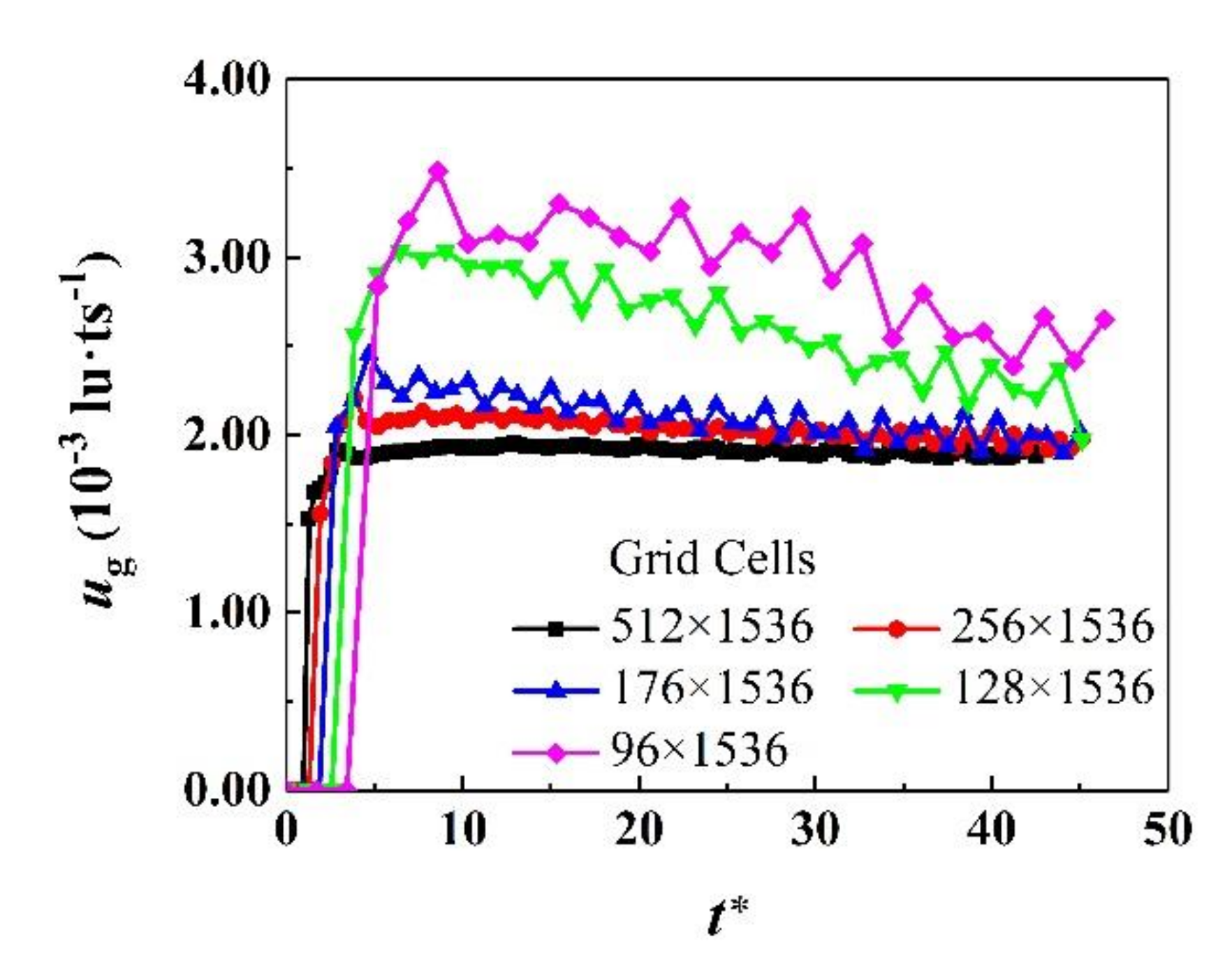
4.2. Grid Independence

The channel structure and the effect of the channel on the bubble are greatly affected by the grid, so the case of the bubble rising in a rectangular channel without particles at ReGr = 100 and Eo = 20 is selected for testing the grid independence. Five different grids with Nx × Ny = 96 × 1536, 128 × 1536, 176 × 1536, 256 × 1536 and 512 × 1536 grid cells are applied in the bubble rising problem, respectively. The number of grid cells in the y-direction is sufficiently large and constant because its influence on the bubble steady velocity is negligible. The rising velocity variation of the bubble with Db = Nx/5 over the dimensionless time is present in Figure 5, and the gravity-based dimensionless time is defined as t * = t G y / D b . It can be observed that when the grid cells are less than 176 × 1536, the bubble terminal velocity is unstable, and the calculation deviation is unacceptable. Thus, the minimum number of grid cells used in the following simulations is set to 176 × 1536.
According to the grid independence test results, considering that the channel width is one of the investigated variables affecting the bubble movement, the two computational domains of wavy and S-shaped channels are discretized using 176 × 1536 to 512 × 1536 and 192 × 1536 to 512 × 1536 grid cells, respectively.

4.3. Mass Conservation

In order to verify the mass conservation of the current model, the evolution of the total system mass versus the dimensionless time is recorded in Figure 6 during a numerical simulation of bubble rising in a wavy vertical channel with L/Db = 0.719 and H/Db = 0.875 at ReGr = 100 and Eo = 20. It is observed that the variation of the normalized total system mass M/M0 is much less than 10−6 over a long period of time, indicating that the mass of the gas-liquid two-phase system is conserved well using current phase-field LB model.

4.4. Channel Width Effect

Undoubtedly, one of the variables that has the most obvious impact on bubble movement in the aforementioned channels is the channel width.
Figure 7 shows the evolution curves of bubbles rising velocity and drag coefficient versus the dimensionless time at ReGr = 100 and Eo = 20. In the wavy vertical channel, the bubble is prone to a stabilized state with a periodically fluctuating terminal velocity, along with CD fluctuating within the certain ranges. In Figure 7, compared with the channel without particles, the rising velocity of the bubble is lower, and the drag coefficient is larger in the channel when the particles are arranged, which indicates that the presence of particles has a significant hindrance to the movement of the bubble.
ug and CD under different channel widths are given in Figure 8, which are calculated by averaging the regularly fluctuating ug and CD over a certain period of time in Figure 7. CD is found to be lower as the channel width becomes wider, and the bubble rises faster. The same results are observed by Patel et al. [38] in the studies on the effects of the amplitude of the sinusoidal channel walls on bubble dynamics. In addition, the horizontal spacing between particles has a more severe impact on the bubble movement than the vertical spacing of the particles. Because the horizontal spacing of the particles directly affects the interaction between the bubble and the particles, and determines the difficulty for the bubble to pass through each gap, while the vertical spacing affects the fluctuation frequency of the bubble drag force, which can only indirectly act on the drag force. In view of this, unless otherwise stated, the following numerical results are obtained from the simulations in the channels with H/Db = 0.875.

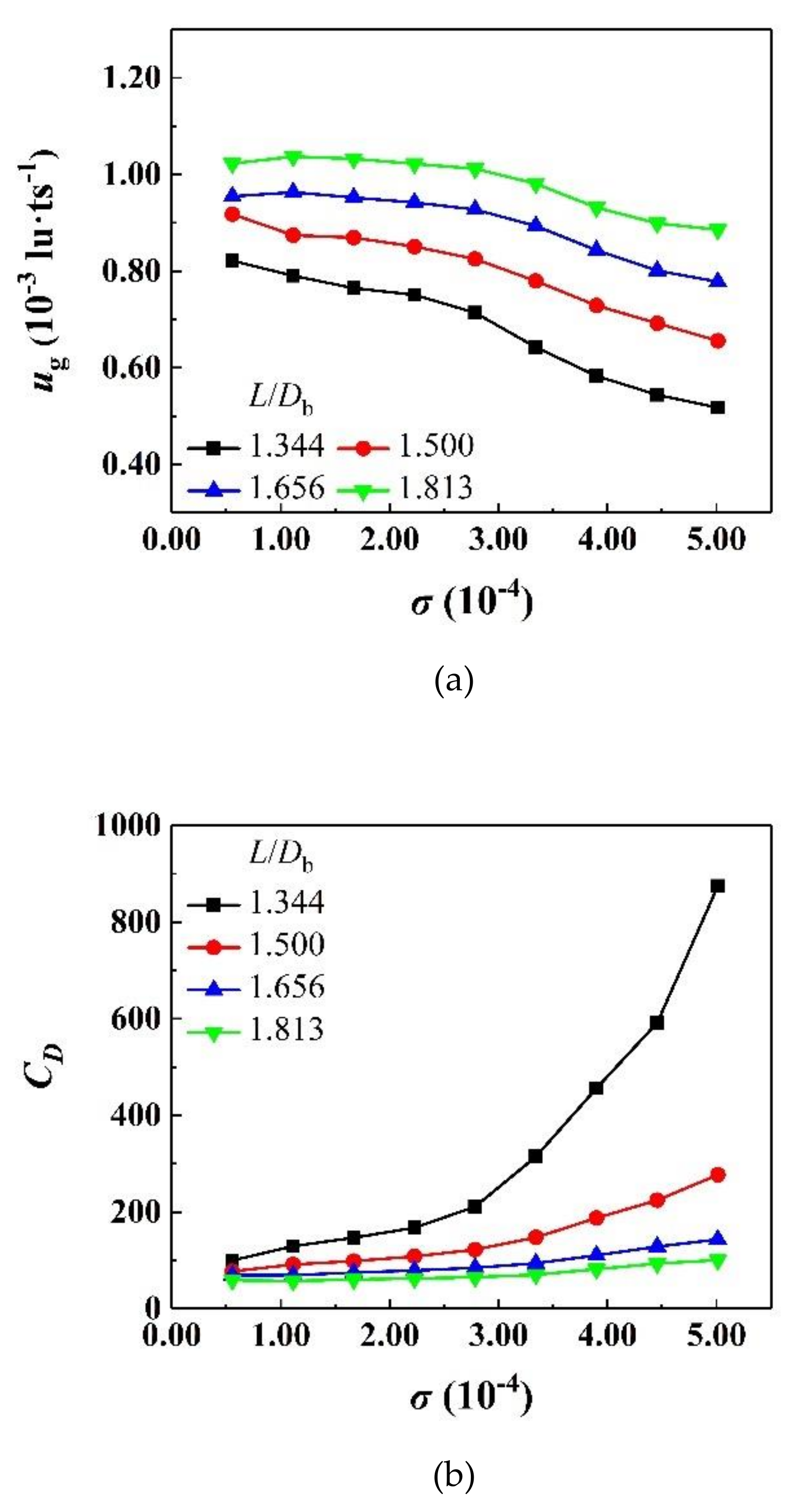
4.5. Surface Tension Effect

Surface tension is an important parameter to characterize the deformation properties of the gas-liquid interface. As for the bubble, a large surface tension means that the bubble is not easy to deform and break. In our study, since the total bubble mass is well conserved, we count the ratio of the total length of the gas-liquid interface to the area occupied by the bubble to measure the deformation rate of the bubble. As shown in Figure 9, the bubble deformation rate is proved to reduce with the increase of surface tension, which confirms that the bubble with large surface tension tends to maintain its original shape and resist deformation.
Furthermore, the declining ug and ascending CD are observed in Figure 10 when the surface tension is gradually increasing. This is because the bubble resists deformation more strongly when colliding with the particles, which restricts the bubble rising velocity. In contrast, the bubble with smaller surface tension is more likely to pass through the narrow gaps in the channel by deforming or even breaking. This phenomenon is consistent with the numerical results of Patel et al. [38], and similar to the studies on the effect of surface tension on liquid penetration by Shi et al. [39].

4.6. Bubble Diameter Effect

The effects of bubble diameter on bubble dynamics are depicted in Figure 11. The bubble diameter in this part is not equivalent to the particle diameter; it varies in the range of 25–204 lu, but the particle diameter is still fixed at 51 lu. Figure 11a indicates that it is more difficult for a bubble with larger diameter to pass through the channel due to the greater blocking effects of the particles, so the bubble rising velocity is slowed down, resulting in the ascent of drag coefficient, as demonstrated in Figure 11b.

4.7. Driving Force Effect

An additional driving force source term Fd can be added to the right side of the governing Equation (4) to simulate the changes in the pressure difference of the packed bed in the actual industry. Here we use the dimensionless ratio Fd/(Gy·ρl) to measure the magnitude of the driving force.
As illustrated in Figure 12, when the incremental additional driving forces are imposed on the bubble based on the presence of buoyancy force, ug increases linearly while CD decreases rapidly. Because the additional driving force pushes the bubble to pass through the channel faster and more smoothly, the rising velocity is significantly increased, so that ug increases and CD decreases.

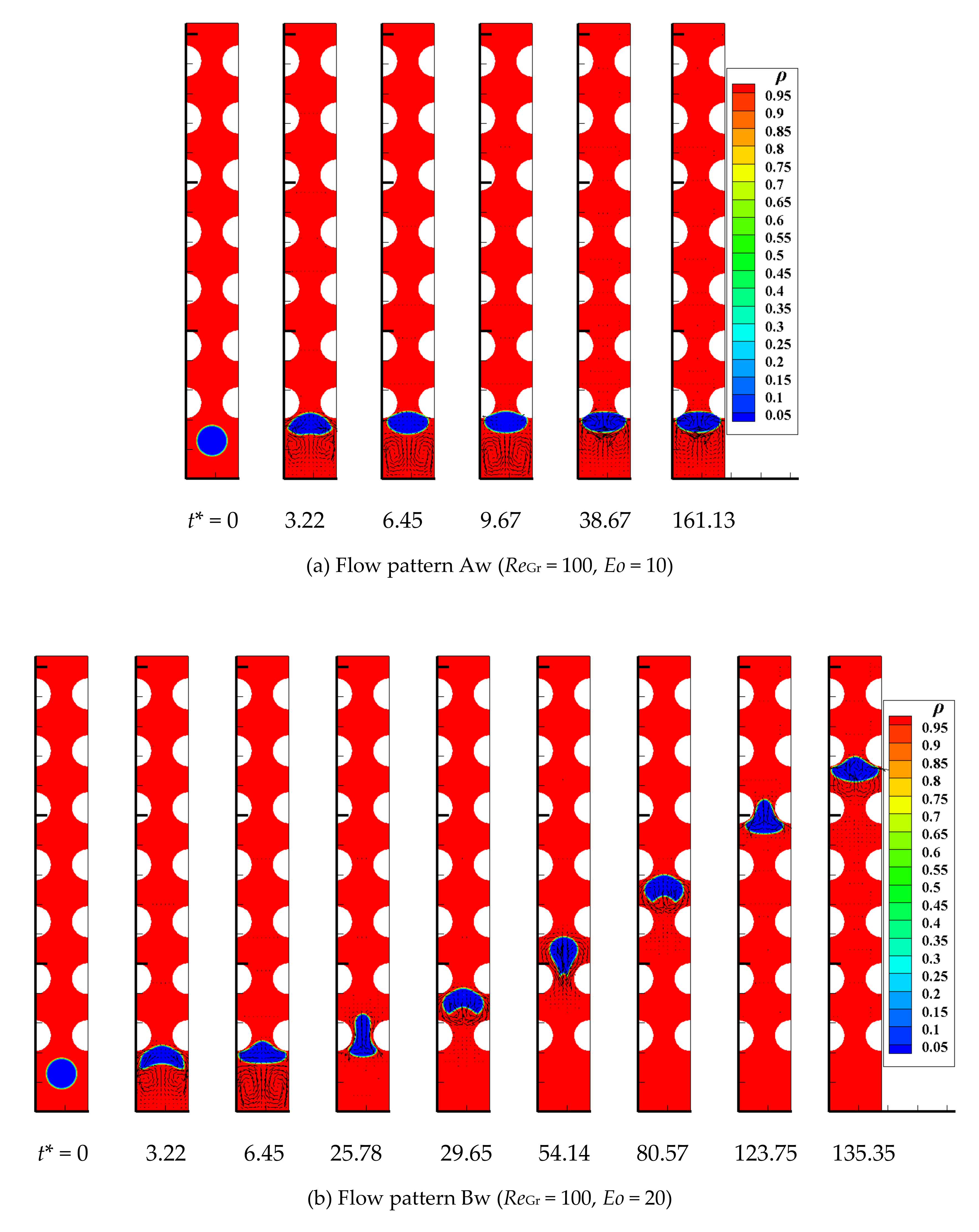
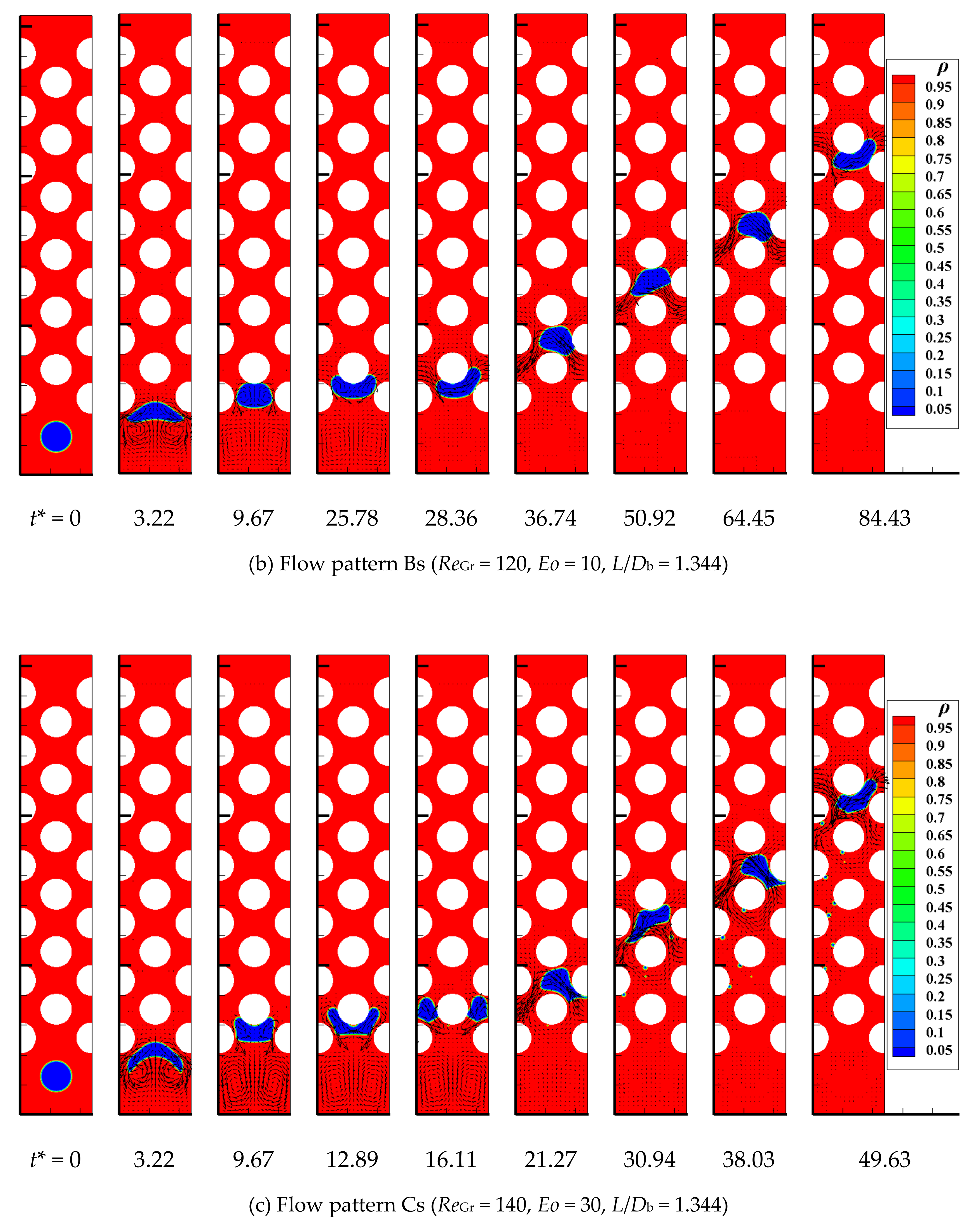
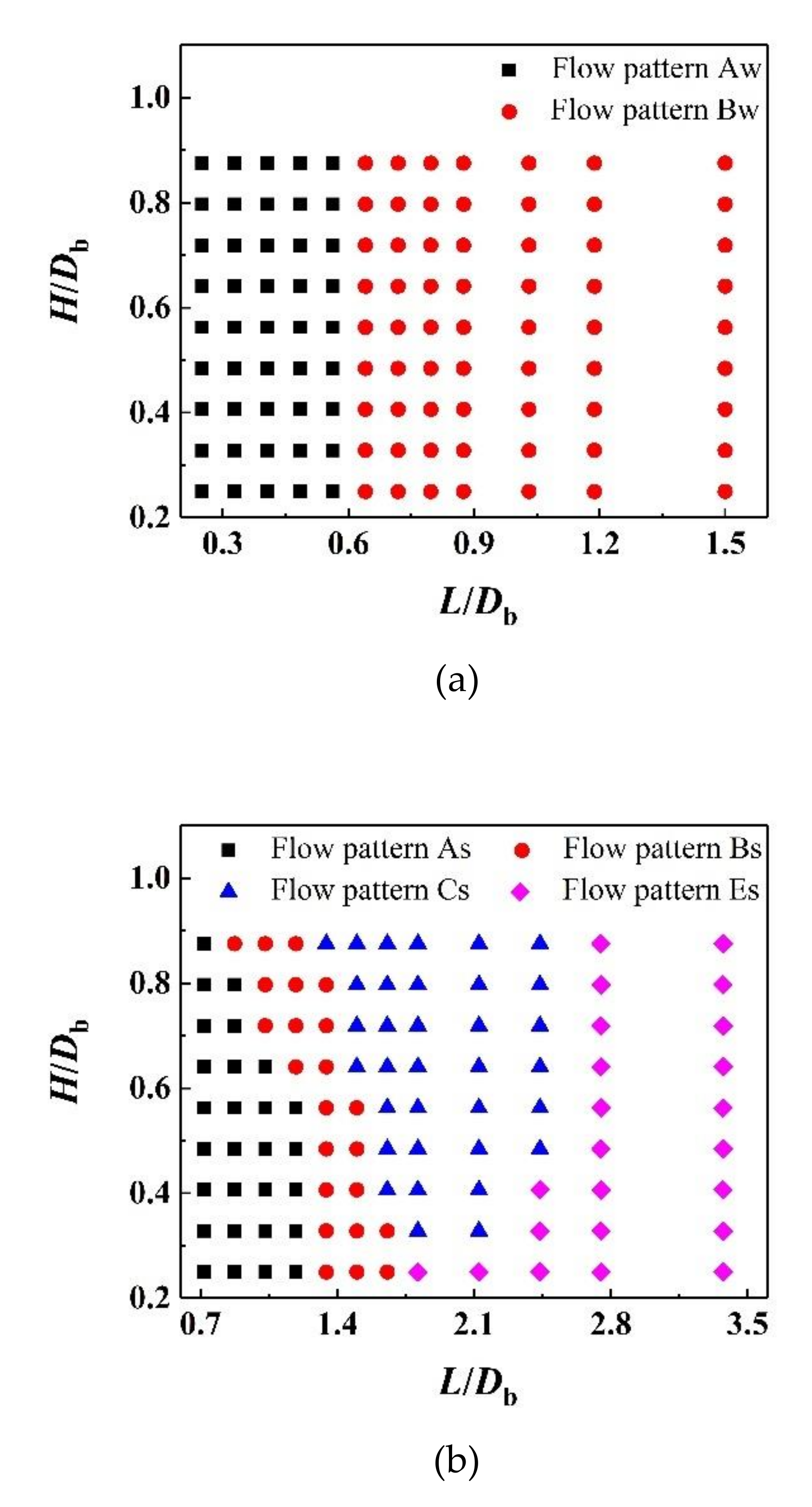
4.8. Bubble Flow Pattern

During the numerical simulations, we found that the fluid properties and operating conditions set in the numerical initializations have significant impacts on the evolutions of the bubble. In order to classify the different bubble evolution processes, the gravity Reynolds number and Eötvös number that include fluid property and operating condition parameters are used as the classification criteria.
For the wavy vertical channel, mainly four types of bubble flow patterns are identified, and their detailed bubble evolution diagrams are listed in Figure 13. The four flow patterns are named Aw, Bw, Cw, and Dw, respectively; their subscript “w” represents the wavy vertical channel, and the capital letters are used to distinguish different flow patterns.
By observing Figure 13, the flow pattern Aw describes that the bubble is completely blocked by the two particles at the entrance of the channel, and even cannot enter the channel. It is inferred from the small Eo that the bubble surface tension in this flow pattern is relatively large, which makes it difficult for the bubble to enter the channel through deformation when encountering obstacles. In contrast, the bubble in the flow pattern Bw will become elongated when it flows into the narrow gaps thanks to the reduced surface tension, thus passing through the channel integrally. In flow pattern Cw, whenever the bubble crosses the gaps and collides with the particles, some secondary bubbles are split from the tail of the parent bubble. Then these secondary bubbles will gradually merge and expand following the parent bubble, and the coalesced secondary bubble with smaller rising resistance will catch up with and merge into the parent bubble finally. As for the flow pattern Dw, compared to the flow pattern Cw, more secondary bubbles are generated after the parent bubble interacts with the particles due to the extremely small surface tension, and the parent bubble will eventually be split into multiple secondary bubbles and dispersed in the liquid. As a summary, a lower Eo leads to a steady rise of the bubble, while a higher Eo instigates the dynamics instability and causes a multiple breakup in the form of secondary bubbles, which is in good agreement with the numerical results of Patel et al. [38] on bubble dynamics in sinusoidal channels using the level set method.
For the S-shaped curved channel, according to different bubble evolutions, five flow patterns As, Bs, Cs, Ds, and Es are distinguished, as illustrated in Figure 14. Among them, flow pattern As is described as the bubble cannot enter and pass through the channel due to the obstruction of the narrow channel. In flow pattern Bs, the bubble enters the channel by being squeezed and elongated, and it shuttles left and right to rise through the channel. For flow patterns As and Bs, the bubbles retain good integrity because of the higher surface tension. As for the flow pattern Cs, the bubble first splits into two after colliding with the particle, and then the two secondary bubbles will coalesce under their interaction. In another case, the two separated secondary bubbles will rise simultaneously with negligible mutual interference due to their far distance, which is named flow pattern Es. Similar to the flow pattern Dw, the bubble in flow pattern Ds is gradually broken into multiple small secondary bubbles and they are dispersed in the liquid phase, continuously breaking and coalescing. It is worth mentioning that the bubbles in the flow patterns Dw and Ds have better dispersibility and higher specific surface area, which are more conducive to gas-liquid mixing and mass transfer in actual industrial production.
In our studies, multiple sets of simulations have been executed within the ReGr range of 0–350 and Eo range of 0–250. Figure 15 depicts the divisions of flow patterns while changing ReGr and Eo with fixed channel widths L/Db = 0.719 and H/Db = 0.875 in the wavy vertical channel and L/Db = 1.344 and H/Db = 0.875 in the S-shaped curved channel. Eo is found to have more significant effects on the flow patterns compared to ReGr, and lower Eo numbers often correspond to the bubbles with higher integrity because the surface tension that is related to Eo number plays a leading role in bubble deformation. In the S-shaped channel, the flow pattern Ds occupies a wider range than the flow pattern Dw in the wavy channel, indicating that the bubbles are more likely to reach the state of fragmentation and dispersion because of more frequent collisions with particles.
It is worth reminding that the trend of the boundaries between different flow patterns in an S-shaped curved channel is similar to the shape regime curve of the single bubble under gravitational motion in the work of Clift et al. [40].
It can be qualitatively summarized from Figure 15 that the bubble becomes more broken and dispersed as ReGr and Eo increase, and this is attributed to the changes in liquid viscosity and bubble surface tension that have significant impacts on the gas-liquid interface. The increase of ReGr and Eo leads to the reduction of liquid viscosity and surface tension, respectively. The reduced liquid viscosity causes the weakening of the viscous effects, which results in the increase of bubble wobbling [38], and the lowered surface tension further promotes bubble deformation and breakup.
In addition to the ReGr and Eo, channel width also has an important influence on the bubble flow patterns. The flow pattern divisions according to the channel widths of two types of channels are demonstrated in Figure 16. The horizontal spacing between particles is found to have more obvious impacts on the flow of bubbles compared to the vertical spacing. The horizontal spacing of the particles directly affects the interaction between the bubble and the particles, thereby affecting the bubble shapes and flow patterns.
On the other hand, in the wavy channel, the changes in channel width do not contribute much to the transitions of bubble flow patterns while maintaining the same ReGr and Eo. Conversely, in the relatively complex S-shaped channel, the transitions of the flow patterns are more sensitive to the variations of channel width; four different flow patterns are revealed by changing the channel width. Under this ReGr and Eo condition, the flow pattern Cs is more conducive to the even distribution of the dispersed phase in practice because too-small channel width is not prone to the disintegration and flow of the dispersed phase, and too large channel width reduces the contact between the dispersed phase and the particles.

5. Conclusions

In this paper, the numerical studies on two-dimensional bubble rising in complex channels saturated with liquid at large density ratios within a wide range of gravity Reynolds numbers and Eötvös numbers have been implemented using phase-field LB model. The main research conclusions of this work are as follows:
(1)
The present LB model is tested through three aspects of Laplace law, bubble deformation, and mass conservation, and it has been proven to have good stability, accuracy, and conservation from both qualitative and quantitative perspectives.
(2)
In the simulations of bubble rising in complex channels, the effects of channel width, surface tension, bubble diameter and additional driving force on bubble motion are investigated in detail. The larger channel width and additional driving force as well as smaller bubble diameter and surface tension lead to lower drag coefficients, which are conducive to smooth passage through the channels for the bubble.
(3)
Four and five types of bubble flow patterns are divided according to different bubble evolution processes under different ReGr, Eo and channel structures conditions in the wavy vertical channel and S-shaped curved channel, respectively. The detailed flow pattern diagrams are drawn for flow pattern recognition. To some extent, this study has some guiding significance for the regulation of bubble flow patterns in the industrial packed beds.

Author Contributions

Conceptualization, Y.Y.; methodology, K.Y.; program execution, K.Y.; validation, K.Y.; investigation, K.Y. and Y.Y.; data curation, K.Y. and Y.Y.; writing—original draft preparation, K.Y.; writing—review and editing, K.Y., Y.Y. and C.Y.; visualization, K.Y.; supervision, Y.Y. and C.Y.; funding acquisition, C.Y. All authors have read and agreed to the published version of the manuscript.

Funding

This work was supported by the National Key Research and Development Program (2019YFC1904204), National Natural Science Foundation of China (21776283, 91934301, 21961160745), External Cooperation Program of BIC, Chinese Academy of Sciences (122111KYSB20190032), and DNL Cooperation Fund, CAS (DNL201902).

Conflicts of Interest

The authors declare no conflict of interest.

Abbreviations

Symbols
csLattice sound speed
CDDrag coefficient
DbBubble diameter
DpParticle diameter
eαLattice-related mesoscopic velocity set
EfVolumetric free energy
EoEötvös number
FαForcing term of the hydrodynamic LBE
FbBody force
FdAdditional driving force
FsSurface tension force
g α eq Equilibrium hydrodynamic distribution function
g ¯ α Modified hydrodynamic distribution function
g ¯ α eq Modified equilibrium hydrodynamic distribution function
GyGravitational acceleration
h α Phase-field distribution function
h α eq Equilibrium phase-field distribution function
HVertical spacing between two vertically adjacent particles
LHorizontal spacing between two horizontally adjacent particles
MMobility
MOrthogonal transformation matrix
MTotal mass of the gas-liquid system
M0Initial total mass of the gas-liquid system
MoMorton number
n ^ Unit vector normal to the gas-liquid interface
n ^ w Unit vector normal to the solid boundary
pMacroscopic pressure
ΔpPressure difference between inside and outside the bubble
RbBubble radius
ReReynolds number of the rising bubble
ReGrGravity Reynolds number
SShortest spacing between two diagonally adjacent particles
S ^ Diagonal relaxation matrix
tTime
t*Gravity-based dimensionless time
uMacroscopic velocity vector
ugBubble rising velocity
wαLattice-related weight coefficient set
xCoordinates of the lattice nodes
xwPosition of the point on the solid boundary
y ^ Unit vector with a vertical downward direction
δtUnit time
δxUnit lattice length
ξInterface thickness
μFluid mixed viscosity
μgGas viscosity
μlLiquid viscosity
μϕChemical potential
ϕPhase-field variable
ϕmPhase field value of the interpolated point
ϕwPhase field value of the point on the solid boundary
ρFluid mixed density
ρgGas density
ρlLiquid density
σSurface tension
τHydrodynamic relaxation time
τϕPhase-field relaxation time
θContact angle
ΩαCollision operator of the hydrodynamic LBE
Ψ(ϕ)Bulk free energy

References

  1. Tailleur, R.G.; Hernandez, J.; Rojas, A. Selective hydrogenation of olefins with mass transfer control in a structured packed bed reactor. Fuel 2008, 87, 3694–3705. [Google Scholar] [CrossRef]
  2. Yuan, R.; He, Z.; Zhang, Y.; Wang, W.; Chen, C.; Wu, H.; Zhan, Z. Partial oxidation of methane to syngas in a packed bed catalyst membrane reactor. AIChE J. 2016, 62, 2170–2176. [Google Scholar] [CrossRef]
  3. Miladinovic, N.; Weatherley, L.R. Intensification of ammonia removal in a combined ion-exchange and nitrification column. Chem. Eng. J. 2008, 135, 15–24. [Google Scholar] [CrossRef]
  4. Huggins, T.M.; Haeger, A.; Biffinger, J.C.; Ren, Z.J. Granular biochar compared with activated carbon for wastewater treatment and resource recovery. Water Res. 2016, 94, 225–232. [Google Scholar] [CrossRef] [Green Version]
  5. Li, Q.; Luo, K.H.; Kang, Q.J.; He, Y.L.; Chen, Q.; Liu, Q. Lattice Boltzmann methods for multiphase flow and phase-change heat transfer. Prog. Energy Combust. Sci. 2016, 52, 62–105. [Google Scholar] [CrossRef] [Green Version]
  6. Gunstensen, A.K.; Rothman, D.H.; Zaleski, S.; Zanetti, G. Lattice Boltzmann model of immiscible fluids. Phys. Rev. A 1991, 43, 4320–4327. [Google Scholar] [CrossRef] [PubMed]
  7. Shan, X.; Chen, H. Lattice Boltzmann model for simulating flows with multiple phases and components. Phys. Rev. E 1993, 47, 1815–1819. [Google Scholar] [CrossRef] [Green Version]
  8. Swift, M.R.; Osborn, W.R.; Yeomans, J.M. Lattice Boltzmann simulation of nonideal fluids. Phys. Rev. Lett. 1995, 75, 830–833. [Google Scholar] [CrossRef] [Green Version]
  9. He, X.; Chen, S.; Zhang, R. A lattice Boltzmann scheme for incompressible multiphase flow and its application in simulation of Rayleigh-Taylor instability. J. Comput. Phys. 1999, 152, 642–663. [Google Scholar] [CrossRef]
  10. Inamuro, T.; Ogata, T.; Tajima, S.; Konishi, N. A lattice Boltzmann method for incompressible two-phase flows with large density differences. J. Comput. Phys. 2004, 198, 628–644. [Google Scholar] [CrossRef]
  11. Lee, T.; Lin, C.L. A stable discretization of the lattice Boltzmann equation for simulation of incompressible two-phase flows at high density ratio. J. Comput. Phys. 2005, 206, 16–47. [Google Scholar] [CrossRef]
  12. Lee, T.; Liu, L. Lattice Boltzmann simulations of micron-scale drop impact on dry surfaces. J. Comput. Phys. 2010, 229, 8045–8063. [Google Scholar] [CrossRef]
  13. Cahn, J.W.; Hilliard, J.E. Free energy of a nonuniform system. I. Interfacial free energy. J. Chem. Phys. 1958, 28, 258–267. [Google Scholar]
  14. Chiappini, D.; Bella, G.; Succi, S.; Toschi, F.; Ubertini, S. Improved lattice Boltzmann without parasitic currents for Rayleigh-Taylor instability. Commun. Comput. Phys. 2010, 7, 423–444. [Google Scholar] [CrossRef]
  15. Guo, Z.; Zheng, C.; Shi, B. Force imbalance in lattice Boltzmann equation for two-phase flows. Phys. Rev. E 2011, 83, 036707. [Google Scholar] [CrossRef]
  16. Zheng, H.W.; Shu, C.; Chew, Y.T. A lattice Boltzmann model for multiphase flows with large density ratio. J. Comput. Phys. 2006, 218, 353–371. [Google Scholar] [CrossRef]
  17. Fakhari, A.; Rahimian, M.H. Phase-field modeling by the method of lattice Boltzmann equations. Phys. Rev. E 2010, 81, 036707. [Google Scholar] [CrossRef]
  18. Fakhari, A.; Lee, T. Finite-difference lattice Boltzmann method with a block-structured adaptive-mesh-refinement technique. Phys. Rev. E 2014, 89, 033310. [Google Scholar] [CrossRef]
  19. Fakhari, A.; Geier, M.; Lee, T. A mass-conserving lattice Boltzmann method with dynamic grid refinement for immiscible two-phase flows. J. Comput. Phys. 2016, 315, 434–457. [Google Scholar] [CrossRef] [Green Version]
  20. Fakhari, A.; Bolster, D. Diffuse interface modeling of three-phase contact line dynamics on curved boundaries: A lattice Boltzmann model for large density and viscosity ratios. J. Comput. Phys. 2017, 334, 620–638. [Google Scholar] [CrossRef] [Green Version]
  21. Fakhari, A.; Mitchell, T.; Leonardi, C.; Bolster, D. Improved locality of the phase-field lattice-Boltzmann model for immiscible fluids at high density ratios. Phys. Rev. E 2017, 96, 053301. [Google Scholar] [CrossRef] [PubMed] [Green Version]
  22. Fakhari, A.; Bolster, D.; Luo, L.S. A weighted multiple-relaxation-time lattice Boltzmann method for multiphase flows and its application to partial coalescence cascades. J. Comput. Phys. 2017, 341, 22–43. [Google Scholar] [CrossRef] [Green Version]
  23. Fakhari, A.; Li, Y.; Bolster, D.; Christensen, K.T. A phase-field lattice Boltzmann model for simulating multiphase flows in porous media: Application and comparison to experiments of CO2 sequestration at pore scale. Adv. Water Resour. 2018, 114, 119–134. [Google Scholar] [CrossRef]
  24. Mitchell, T.; Leonardi, C.; Fakhari, A. Development of a three-dimensional phase-field lattice Boltzmann method for the study of immiscible fluids at high density ratios. Int. J. Multiph. Flow 2018, 107, 1–15. [Google Scholar] [CrossRef] [Green Version]
  25. Magaletti, F.; Picano, F.; Chinappi, M.; Marino, L.; Casciola, C.M. The sharp-interface limit of the Cahn-Hilliard/Navier-Stokes model for binary fluids. J. Fluid Mech. 2013, 714, 95–126. [Google Scholar] [CrossRef]
  26. Chiu, P.H.; Lin, Y.T. A conservative phase field method for solving incompressible two-phase flows. J. Comput. Phys. 2011, 230, 185–204. [Google Scholar] [CrossRef]
  27. Jacqmin, D. Calculation of two-phase Navier-Stokes flows using phase-field modeling. J. Comput. Phys. 1999, 155, 96–127. [Google Scholar] [CrossRef]
  28. Jacqmin, D. Contact-line dynamics of a diffuse fluid interface. J. Fluid Mech. 2000, 402, 57–88. [Google Scholar] [CrossRef]
  29. Geier, M.; Fakhari, A.; Lee, T. Conservative phase-field lattice Boltzmann model for interface tracking equation. Phys. Rev. E 2015, 91, 063309. [Google Scholar] [CrossRef] [Green Version]
  30. He, X.; Luo, L.S. Theory of the lattice Boltzmann method: From the Boltzmann equation to the lattice Boltzmann equation. Phys. Rev. E 1997, 56, 6811–6817. [Google Scholar] [CrossRef] [Green Version]
  31. Lallemand, P.; Luo, L.S. Theory of the lattice Boltzmann method: Dispersion, dissipation, isotropy, Galilean invariance, and stability. Phys. Rev. E 2000, 61, 6546–6562. [Google Scholar] [CrossRef] [Green Version]
  32. Yu, D.; Mei, R.; Shyy, W. A unified boundary treatment in lattice Boltzmann method. AIAA J. 2003. [Google Scholar] [CrossRef]
  33. Hua, J.; Lou, J. Numerical simulation of bubble rising in viscous liquid. J. Comput. Phys. 2007, 222, 769–795. [Google Scholar] [CrossRef]
  34. Fakhari, A.; Rahimian, M.H. Simulation of an axisymmetric rising bubble by a multiple relaxation time lattice Boltzmann method. Int. J. Mod. Phys. B 2009, 23, 4907–4932. [Google Scholar] [CrossRef]
  35. Huang, H.; Huang, J.J.; Lu, X.Y. A mass-conserving axisymmetric multiphase lattice Boltzmann method and its application in simulation of bubble rising. J. Comput. Phys. 2014, 269, 386–402. [Google Scholar] [CrossRef]
  36. Liang, H.; Li, Y.; Chen, J.; Xu, J. Axisymmetric lattice Boltzmann model for multiphase flows with large density ratio. Int. J. Heat Mass Transf. 2019, 130, 1189–1205. [Google Scholar] [CrossRef] [Green Version]
  37. Bhaga, D.; Weber, M.E. Bubbles in viscous liquids: Shapes, wakes and velocities. J. Fluid Mech. 1981, 105, 61–85. [Google Scholar] [CrossRef] [Green Version]
  38. Patel, T.; Patel, D.; Thakkar, N.; Lakdawala, A. A numerical study on bubble dynamics in sinusoidal channels. Phys. Fluids 2019, 31, 052103. [Google Scholar] [CrossRef]
  39. Shi, Y.; Tang, G.H.; Lin, H.F.; Zhao, P.X.; Cheng, L.H. Dynamics of droplet and liquid layer penetration in three-dimensional porous media: A lattice Boltzmann study. Phys. Fluids 2019, 31, 042106. [Google Scholar] [CrossRef]
  40. Clift, R.; Grace, J.R.; Weber, M.E. Bubbles, Drops, and Particles; Academic Press: New York, NY, USA, 1978. [Google Scholar]
Figure 1. Schematic of curved boundary treatment.
Processes 08 01608 g001
Figure 2. Phase field distribution contour (a) of the stable bubble and phase field distribution comparison in the radial direction (b) through the bubble.
Processes 08 01608 g002
Figure 3. Relationship between pressure difference, surface tension, and radius of the bubble.
Processes 08 01608 g003
Figure 4. Schematics of wavy vertical channel (a) and S-shaped curved channel (b).
Processes 08 01608 g004
Figure 5. Variations of the bubble rising velocity with dimensionless time using five different grids.
Processes 08 01608 g005
Figure 6. Variation of the normalized total system mass with dimensionless time.
Processes 08 01608 g006
Figure 7. Variations of ug (a) and CD (b) with dimensionless time at ReGr = 100 and Eo = 20.
Processes 08 01608 g007
Figure 8. Variations of ug (a) and CD (b) with channel width at ReGr = 100 and Eo = 20.
Processes 08 01608 g008
Figure 9. Variation of bubble deformation rate with surface tension at ReGr = 100 and Eo = 20.
Processes 08 01608 g009
Figure 10. Variations of ug (a) and CD (b) with surface tension at ReGr = 100 and Eo = 20.
Processes 08 01608 g010
Figure 11. Variations of ug (a) and CD (b) with bubble diameter at ReGr = 100 and Eo = 20.
Processes 08 01608 g011
Figure 12. Variations of ug (a) and CD (b) with additional driving force at ReGr = 100 and Eo = 20.
Processes 08 01608 g012
Figure 13. Bubble evolution diagrams of flow patterns Aw (a), Bw (b), Cw (c), and Dw (d) in the wavy vertical channel with L/Db = 0.719.
Processes 08 01608 g013aProcesses 08 01608 g013b
Figure 14. Bubble evolution diagrams of flow patterns As (a), Bs (b), Cs (c), Ds (d), and Es (e) in the S-shaped curved channel.
Processes 08 01608 g014aProcesses 08 01608 g014bProcesses 08 01608 g014c
Figure 15. Flow pattern divisions according to ReGr and Eo in the wavy vertical channel (a) and S-shaped curved channel (b).
Processes 08 01608 g015
Figure 16. Flow pattern divisions according to the channel widths of the wavy vertical channel (a) and S-shaped curved channel (b) at ReGr = 100 and Eo = 20.
Processes 08 01608 g016
Table 1. Comparison of terminal bubble shapes observed in experiments and predicted by front tracking method, previous and present LBMs.
CaseReGrEoExperiments (Bhaga and Weber, 1981) [37]Front Tracking Method (Hua and Lou, 2007) [33]LBM (Liang et al., 2019) [36]Present LBM
A11.6717.7 Processes 08 01608 i001 Processes 08 01608 i002 Processes 08 01608 i003 Processes 08 01608 i004
A279.8832.2 Processes 08 01608 i005 Processes 08 01608 i006 Processes 08 01608 i007 Processes 08 01608 i008
A3134.63115 Processes 08 01608 i009 Processes 08 01608 i010 Processes 08 01608 i011 Processes 08 01608 i012
A430.83339 Processes 08 01608 i013 Processes 08 01608 i014 Processes 08 01608 i015 Processes 08 01608 i016
A549.72641 Processes 08 01608 i017 Processes 08 01608 i018 Processes 08 01608 i019 Processes 08 01608 i020
Table 2. Comparison of Re obtained from the present LBM and the experimental results.
CaseRe of Experiments [37]Re of Present LBMRelative Error (%)
A10.2320.2119.05
A255.347.813.56
A394.087.56.91
A418.316.410.38
A530.327.59.24
Publisher’s Note: MDPI stays neutral with regard to jurisdictional claims in published maps and institutional affiliations.

