Study of Dynamics of Heat Transfer in the Flat-Plate Solar Collector

Abstract

Flat plate solar collector has been presented as an example of a heat-exchanger with two input signals, solar radiation intensity and temperature of working medium on the input, and one output signal, the temperature of a working medium on the output. The dynamics of heat exchange were analyzed for two models of a solar collector—an analog one using a thermoelectric analogy, and a digital one—determined experimentally in on-line mode using the parametric identification method. The characteristics of both models were compared in terms of their step and frequency response for selected construction and operational parameters. Tests of step responses determined for the analog model indicate that the dynamics of heat exchange in the solar collector depending on two input signals is varied. For step-forcing of input signals of the analog model, in both cases, a stable steady state is achieved, but while the first of the signals is inertial, the second one is oscillatory. The phenomenon of temperature oscillation at the collector outlet suggests the need to introduce a new physical quantity in the thermoelectric analogy-thermal inductance. Such an assessment of the dynamics of the solar collector can be useful for proper designing (construction parameters simulation) and diagnostics (operational parameters simulation) of the device.

1. Introduction

The main tasks of solar systems are effectively collection, processing, and accumulation of solar energy. It is connected with the need to recognize the thermal processes occurring in the solar collector, as well as to define the impact of the device construction and/or operational parameters on these processes. This task is connected not only with proper design of the components of such a system but also with automation of its functioning, especially if it is one of the segments of hybrid energy system (HES) [1,2]. The solution of control and regulation problems requires identification of dynamic properties of all cooperating component appliances, even at the stage of designing them best. Summarizing, proper recognition of heat transfer phenomena occurring in the solar collector in relation to construction and operational device parameters is directly related to the identification of the impact of these parameters on the dynamics of device operation. Therefore, this publication presents the dynamics of heating up of solar collector’s working medium.

In the available studies, mathematical and physical models of solar collector are theoretical [3,4], based on energy balance differential equations. There are also digital models created on the basis of data from long-term measurements (monitoring system) [5,6].

In the papers [7,8], the dynamic properties of collector have been specified by the determination of heating characteristics of working medium with the assumption that solar radiation is the only input excitation signal and temperature at the collector’s output is the output signal. The characteristics can be specified theoretically or experimentally. The theoretical characteristics is a solution of a differential equation describing heat transfer in the non-steady state [9,10]. Introducing certain simplifying assumptions is its disadvantage, but the possibility of conducting simulation research is its advantage. The step responses determined experimentally requires the measurements of temperature changes over time on the real object [11]. Time consumption and cost consumption are disadvantages of such a solution. Other elements of a solar heating installation are sometimes included in a steering block diagram, e.g., a hot water storage tank [12].

In automation, a solar collector is most often treated as a heating object with the inertial nature [13]. By analyzing the device frequency response, the recognition of dynamic properties in more detail is possible. Analysis of frequency responses is not widely common in solar collector modeling. More common is describing of solar radiation conditions using frequency characteristics for dynamic modeling of solar collector and heat exchanger [14,15,16]. A solar collector certainly can be treated as a heat exchanger.

The scientific literature describes the analysis of the impact of changes in solar collector parameters on device efficiency [17]. Additionally, the analyses on the influence of changes in the construction parameters on the collector efficiency and the working medium temperature rise not only in relation to flat-plate, vacuum tube but also in relation to the air collectors, parabolic trough collectors. Even the collectors made of plastic and concrete are performed as a result of simulation tests [18,19,20,21,22,23,24,25,26,27,28].

In addition to the construction parameters, there are analyses of operating parameters, such as: solar collector tilt angle [18,29], the volumetric flow rate of working medium [30] or working medium mass flow rate [28,31], and even the influence of weather conditions on device’s efficiency [32]. In addition, the influence of the wind speed and flow rate of the working medium on the final outlet temperature has been studied for years [33]. The analyses concern the basic solar heating systems for water heating [34,35] and more complex hybrid [36] or industrial ones [37].

The application of analog model proposed by the Aleksiejuk et al. in [6] gives the possibility to simulate changes in solar collector construction and operational parameters without need for time-consuming and cost-consuming experiments. This publication presents the impact of changes in construction and operational parameters on the dynamics of heating up of solar collectors working medium.

In the process of designing or diagnostics of solar heating systems the collector plays a major role. It is important to choose such a level of detail in the model in order to be able to distinguish the influence of particular construction and operating parameters of a solar collector on the dynamics of the device. So far, the proposed models are first order models and treat the solar collector as a homogeneous body and therefore they are first-order models [11,13]. The article presents the application of the solar collector analog model, which distinguishes three homogeneous bodies: glass cover, absorber plate, and working medium. Hence, the analog model presented in the article is a third-order model. Two models in the form of electric four-terminal networks have been developed for the analysis of collector operation dynamics. They have one input signal (solar radiation intensity and, alternatively, the temperature of working medium on the collector input) and one output signal (temperature of the working medium on the collector output). In automation, such models are referred to as SISO (single input single output).

2. Materials and Methods

Both the analog and digital model were presented for the same device—flat plate solar collector. The flat plate solar collector is a part of an HES. Tested system is used to prepare hot water for the hotel and utility building. In addition to flat plate solar collectors, the HES includes vacuum tube solar collectors and heat pump, for which the lower energy source is a vertical ground exchanger (Figure 1). The main hot utility water tank has a capacity of 1000 dm³, and a supplementary one 300 dm³. The solar installation supplies thermal energy to a 2000 dm³ tank, which, in turn, serves as energy storage for the heat pump. The HES is fully monitored, and the results of measurements of all the physical quantities (temperature, intensity of solar radiation, flow rate of working media, etc.) are registered daily with a resolution of one minute [38].

The authors have used the method of equivalent thermal network (ETN) based on thermoelectric analogy for building the analog model of a flat plate solar collector [6]. The analysis of heat exchange in a solar collector was carried out by solving an electrical circuit (Figure A1). Two collector models were developed, transforming its basic electrical circuit into two four-terminal networks, in which one input and one output signal (SISO models) were distinguished. The input signals are the solar radiation intensity P(t) and the input temperature of the working medium T_fin(t) and the output signal is the output temperature of the working medium T_fout(t). This allows the influence of the input signals on the collector dynamics to be analyzed separately.

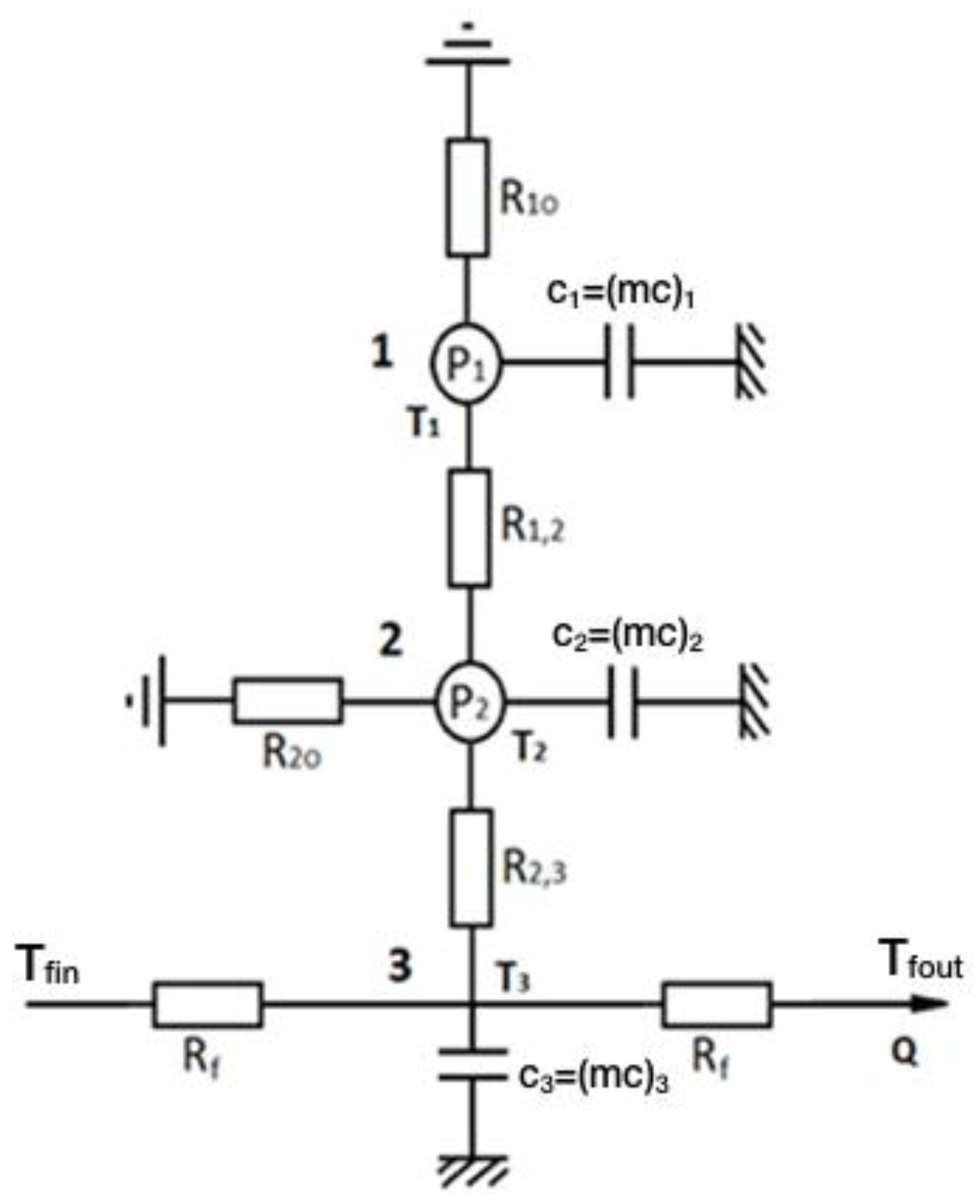
The assumption adopted in the construction of the electric circuit diagram of the collector is to divide the collector into three homogeneous bodies whose physical properties are concentrated in the nodes of the circuit, respectively: 1—glass cover, 2—absorber plate, and 3—working medium. Nodes 1, 2, and 3 are connected with each other and the environment by thermal resistance. Heat streams flow between the nodes and the environment. Each node has been assigned a corresponding heat capacity C_i = (mc)_i. The transient heat exchange is described in Equation (1):

$$C\frac{d\overline{T}\left(t\right)}{dt}+\mathsf{\Lambda }\overline{T}\left(t\right) = \overline{P}\left(t\right)$$

(1)

where:

$$C=\left[\begin{array}{ccc}{\left(mc\right)}_1& 0& 0\\ 0& {\left(mc\right)}_2& 0\\ 0& 0& {\left(mc\right)}_3\end{array}\right]; \overline{T}=\left[\begin{array}{c}{T}_1\\ T_2\\ T_3\end{array}\right]; \overline{P}=\left[\begin{array}{c}{P}_1+\frac{T_o}{R_{1,0}}\\ P_2+\frac{T_o}{R_{20}}\\ \frac{T_{fin}}{R_f}\end{array}\right]$$

(2)

$$\mathsf{\Lambda } =\left[\begin{array}{ccc}{\mathsf{\Lambda }}_{1,1}& {\mathsf{\Lambda }}_{1,2}& {\mathsf{\Lambda }}_{1,3}\\ {\mathsf{\Lambda }}_{2,1}& {\mathsf{\Lambda }}_{2,2}& {\mathsf{\Lambda }}_{2,3}\\ {\mathsf{\Lambda }}_{3,1}& {\mathsf{\Lambda }}_{3,2}& {\mathsf{\Lambda }}_{3,3}\end{array}\right] = \left[\begin{array}{ccc}\frac{1}{R_{1,2}}+\frac{1}{R_{1,0}}& -\frac{1}{R_{1,2}}& 0\\ -\frac{1}{R_{1,2}}& \frac{1}{R_{1,2}}+\frac{1}{R_{2,3}}+\frac{1}{R_{2o}}& -\frac{1}{R_{2,3}}\\ 0& -\frac{1}{R_{2,3}}& \frac{1}{R_{2,3}}+\frac{1}{R_f}\end{array}\right]$$

(3)

The basic circuit diagram on the basis of which the four-terminal networks were developed and solved is shown in Appendix A in Figure A1 and described in detail in [6]. Dynamic properties of the modeled collector are represented by the operator transmissions of two electric four-terminal networks. It was determined using Laplace transformation for a differential equation describing the dependence of the output signal on the input signal for a given four-terminal network. The collector can be presented as two separate SISO models represented by Equations (4) and (5):

$$G1\left(s\right)=\frac{T_{fout}\left(s\right)}{P\left(s\right)}=\frac{b_1^{\prime }s+b_0^{\prime }}{s^3+a_2^{\prime }{s}^2+a_1^{\prime }s+a_0^{\prime }}$$

(4)

and

$$G2\left(s\right)=\frac{T_{fout}\left(s\right)}{T_{fin}\left(s\right)}= \frac{b_2^{\prime \prime }{s}^2+b_1^{\prime \prime }s+b_0^{\prime \prime }}{s^3+a_2^{\prime \prime }{s}^2+a_1^{\prime \prime }s+a_0^{\prime \prime }}$$

(5)

transfer functions describing the relationships between the particular input (in)/output (out) signals: P(s)—transform of solar radiation intensity, T_f(s)—transform of working medium temperature. The coefficients of both the transfer functions depend on resistances and heat capacities of mentioned above flat plate solar collector (

Table A1. Description of resistances and heat capacities of a modeled flat-plate solar collector.

Symbol and Description	Unit
R10—resistance to glass conductivity and heat transfer from the outer surface of the glass cover to the ambient environment	K/W
R12—resistance between glass cover and absorber	K/W
R23—resistance being the sum of resistance to conductivity through the absorber and to transfer to the working medium	K/W
R20—resistance being the total resistance of conductivity through the insulation surface, air gap and heat transfer to the ambient environment from the bottom surface of the collector	K/W
Rf—thermal resistance of the working medium	K/W
Rλs—thermal resistance through the glass	K/W
Rαs—thermal resistance from the outer surface of the glass cover	K/W
Ras—thermal resistance between the absorber and the inner surface of the glass cover	K/W
Rλa—thermal resistance through the absorber	K/W
Rα—thermal resistance through the working medium	K/W
Rλp—thermal resistance through the total air gap	K/W
Rλiz—thermal resistance through the insulation	K/W
Rλd—thermal resistance through the collector bottom casing	K/W
Rαd—thermal resistance from the external bottom casing to the environment	K/W
αas—heat transfer coefficient between the absorber and the inner surface of the glass cover	W/(m2∙K)
αs—heat transfer coefficient from the external surface of the glass cover	W/(m2∙K)
αd—heat transfer coefficient for the bottom casing of the collector	W/(m2∙K)
α—heat transfer coefficient of the working medium	W/(m2∙K)
λs—thermal conductivity of glass	W/(m∙K)
λ—thermal conductivity of working medium	W/(m∙K)
λa—thermal conductivity of absorber material	W/(m∙K)
λp—thermal conductivity of air	W/(m∙K)
λiz—thermal conductivity of insulation material	W/(m∙K)
λd—thermal conductivity of bottom casing material	W/(m∙K)
σs—glass thickness	m
σa—absorber thickness	m
σiz—insulation thickness	m
σd—bottom casing thickness	m
Σσp—total air gap between the absorber and the insulation and the insulation and the bottom casing of the collector	m
Ss—glass cover surface	m2
Sas—arithmetic mean of Sa and Ss	m2
Sk—total internal surface area of the flow channels of the absorber	m2
Sa—absorber surface	m2
Sd—bottom casing surface	m2
cp—specific heat of the working medium	J/(m3∙K)
Q—working medium flow	m3/s
mc1—heat capacity of the glass cover	J/K
mc2—heat capacity of the absorber	J/K
mc3—heat capacity of the working medium	J/K

,

Table A2. List of equations used for thermal resistances and heat capacities calculation.

Equations	Number
R1,o = Rλs + Rαs	(A1)
Rλs = $\frac{0,5{\delta }_s}{{\lambda }_s{S}_s}$	(A2)
Rαs = $\frac{1}{{\alpha }_s{S}_s}$	(A3)
R1,2 = Rλs + Ras	(A4)
Ras = $\frac{1}{{\alpha }_{as}{S}_{as}}$	(A5)
R2,3 = Rλa + Rα	(A6)
Rλa = $\frac{{\delta }_a}{{\lambda }_a{S}_k}$	(A7)
Rα = $\frac{1}{\alpha S_k}$	(A8)
R2,o = Rλp + Rλiz + Rλd + Rαd	(A9)
Rλp = $\frac{\sum {\delta }_p}{{\lambda }_p{S}_a}$	(A10)
Rλiz = $\frac{{\delta }_{iz}}{{\lambda }_{iz}{S}_a}$	(A11)
Rλd = $\frac{{\delta }_d}{{\lambda }_d{S}_d}$	(A12)
Rαd = $\frac{1}{{\alpha }_d{S}_d}$	(A13)
Rf = $\frac{1}{2 c_{p}Q}$	(A14)
${\left(mc\right)}_1=c_s·{\rho }_s·S_s·{\sigma }_s$	(A15)
${\left(mc\right)}_2=c_a·{\rho }_a·S_a·{\sigma }_a$	(A16)
${\left(mc\right)}_3=c_p·V_l$	(A17)

,

Table A3. Transfer function coefficients of the first segment $G1\left(s\right)=\frac{b_1^{\prime }s+b_0^{\prime }}{s^3+a_2^{\prime }{s}^2+a_1^{\prime }s+a_0^{\prime }}$ where: p_g—glass transmittance, a_a—absorber absorptivity, a_g—glass absorptivity.

Coefficient	Description
b′1	$\frac{p_g·a_a·\frac{1}{S_a}·R_{12}·R_{10}·m{c}_1}{R_{12}·R_{10}·R_{23}·m{c}_1·m{c}_2·m{c}_3}$
b′0	$\frac{\left(a_g·\frac{1}{S_g}+p_g·a_a·\frac{1}{S_a}\right)·R_{10}+p_g·a_a·\frac{1}{S_a}·R_{12}}{R_{12}·R_{10}·R_{23}·m{c}_1·m{c}_2·m{c}_3}$
a′2	$\frac{R_{10}·R_{23}·m{c}_1·m{c}_3+R_{12}·R_{23}·m{c}_2·m{c}_3+\left(\frac{R_{10}·R_{12}}{R_{20}}\right)·R_{23}·m{c}_1·m{c}_3+R_{10}·R_{23}·m{c}_2·m{c}_3+R_{10}·R_{12}·m{c}_1·m{c}_2·\left(\frac{R_{23}}{R_f}\right)+R_{10}·R_{12}·m{c}_1·m{c}_2}{R_{12}·R_{10}·R_{23}·m{c}_1·m{c}_2·m{c}_3}$
a′1	$\frac{R_{23}\ast \left(\frac{R_{12}}{R_{20}}\right)·m{c}_3+R_{23}·\left(\frac{R_{10}}{R_{20}}\right)\ast m{c}_3+R_{23}·m{c}_3+R_{10}·m{c}_1·\left(\frac{R_{23}}{R_f}\right)+R_{12}·m{c}_2·\left(\frac{R_{23}}{R_f}\right)+\left( \frac{R_{10}\ast R_{12}}{R_{20}}\right)·\left( \frac{R_{23}}{R_f}\right)·m{c}_1+R_{10}·m{c}_2·\left(\frac{R_{23}}{R_f}\right)+R_{10}·m{c}_1+R_{12}·m{c}_2+\left(\frac{R_{10}\ast R_{12}}{R_{20}}\right)·m{c}_1+R_{10}·m{c}_2}{R_{12}·R_{10}·R_{23}·m{c}_1·m{c}_2·m{c}_3}$
a′0	$\frac{\left(\frac{R_{12}}{R_{20}}\right)·\left( \frac{R_{23}}{R_f}\right)+\left( \frac{R_{10}}{R_{20}}\right)·\left( \frac{R_{23}}{R_f}\right)+\frac{R_{23}}{R_f}+\frac{R_{12}}{R_{20}}+\frac{R_{10}}{R_{20}}+1}{R_{12}·R_{10}·R_{23}·m{c}_1·m{c}_2·m{c}_3}$

and

Table A4. Transfer function coefficients of the second segment $G2\left(s\right)=\frac{b_2^{\prime \prime }{s}^2+b_1^{\prime \prime }s+b_0^{\prime \prime }}{s^3+a_2^{\prime \prime }{s}^2+a_1^{\prime \prime }s+a_0^{\prime \prime }}$.

Coefficient	Description
b″	$\frac{R_{23}·R_{12}·R_{10}·R_{20}·m{c}_1·m{c}_2}{R_f·R_{12}·R_{10}·R_{23}·R_{20}·m{c}_1·m{c}_2·m{c}_3}$
b″1	$\frac{R_{12}·R_{10}·R_{20}·m{c}_1+R_{23}·R_{10}·R_{20}·m{c}_2+R_{23}·R_{12}·R_{10}·m{c}_1+R_{23}·R_{12}·R_{20}·m{c}_2+R_{23}·R_{20}·R_{10}·m{c}_1}{R_f·R_{12}·R_{10}·R_{23}·R_{20}·m{c}_1·m{c}_2·m{c}_3}$
b″0	$\frac{R_{10}·R_{20}+R_{12}·R_{20}+R_{23}·R_{10}+R_{23}·R_{12}·R_{23}·R_{20}}{R_f·R_{12}·R_{10}·R_{23}·R_{20}·m{c}_1·m{c}_2·m{c}_3}$
a″2	$\frac{R_{23}·R_{10}·R_{20}·m{c}_1·m{c}_2+R_f·R_{12}·R_{10}·R_{20}·m{c}_1·m{c}_3+R_f·R_{23}·R_{10}·R_{20}·m{c}_2·m{c}_3+R_f·R_{23}·R_{12}·R_{10}·m{c}_1·m{c}_3+R_f·R_{23}·R_{12}·R_{20}·m{c}_2·m{c}_3+R_f·R_{23}·R_{20}·R_{10}·m{c}_1·m{c}_3+R_f·R_{12}·R_{10}·R_{20}·m{c}_1·m{c}_2}{R_f·R_{12}·R_{10}·R_{23}·R_{20}·m{c}_1·m{c}_2·m{c}_3}$
a″1	$\frac{R_{12}·R_{10}·R_{20}·m{c}_1+R_{23}·R_{10}·R_{20}·m{c}_2+R_{23}·R_{12}·R_{10}·m{c}_1+R_{23}·R_{12}·R_{20}·m{c}_2+R_{23}·R_{20}·R_{10}·m{c}_1+R_f·R_{10}·R_{20}·m{c}_3+R_f·R_{12}·R_{20}·m{c}_3+R_f·R_{23}·R_{10}·m{c}_3+R_f·R_{23}·R_{12}·m{c}_3+R_f·R_{23}·R_{20}·m{c}_3+R_f·R_{10}·R_{20}·m{c}_2+R_f·R_{12}·R_{10}·m{c}_1+R_f·R_{12}·R_{20}·m{c}_2+R_f·R_{20}·R_{10}·m{c}_1}{R_f·R_{12}·R_{10}·R_{23}·R_{20}·m{c}_1·m{c}_2·m{c}_3}$
a″0	$\frac{R_{10}·R_{20}+R_{12}·R_{20}+R_{23}·R_{10}+R_{23}·R_{12}+R_{23}·R_{20}+R_f·R_{12}+R_f·R_{20}+R_f·R_{10}}{R_f·R_{12}·R_{10}·R_{23}·R_{20}·m{c}_1·m{c}_2·m{c}_3}$

. The polynomial degree of the denominator in both transfer functions G1(s) and G2(s) is of the third degree. In this publication, the analog model has been applied for simulation the changes in construction and operational parameters of a flat plate solar collector. It was a theoretical simulation. For the method verification, analog model was compared to the results achieved for the digital model described in detail in [6].

A digital model was developed on the basis of a database of the real measurement results of the hybrid energy system. The method of parametric identification has been used for building the digital model; it models the process of the output signal on the basis of measurement results registered in online mode. It also allows for determining the dynamics of the modeled object by determining transfer function (G1′(s), G2′(s) according to the analog model) and step responses on its basis. The applied IT tool was MATLAB package System Identification Toolbox (SIT). ARX [n_a,n_b,n_k], the most frequently recommended one for modeling, has been selected from among the ones proposed for applying in the package of parametric models. The best matching with the process of the input signal has been the selection criterion of a parametric model, which corresponds to the minimization of the value of root mean square error (RMS). In this publication the accuracy of digital model has been increased. The process of selecting the appropriate digital model is described below. Selected model is the one with the highest degree of fit to the actual measurements.

Due to fact that the polynomial degree of the denominator in both transfer functions G1′(s), G2′(s), is of the third degree (the same as for the analog model), attention has been paid to whether we achieve minimization for the RMS error for the digital model with n_a = 3.

The choice of n_k parameter connected with the measurements of the analyzed phenomenon is very important. The correct increment of temperature of the working medium ΔT_f = T_fout − T_fin, being the difference between temperature measured on the output of the collector T_fout and on the input T_fin, requires taking into account certain delay time in reading the measurement results of both temperatures [39,40,41]. It is connected with the time of working medium flowing through the collector. This time depends on the length of the flow canal and the yield of the working medium (working medium flow rate). The difference of temperature values on the input and output of the collector cannot be from the same moment of time. The more slowly the working medium flows, the higher temperature it heats to, but the delay of reading temperature on the output is higher. And the other way around, if the length of the stream of working medium is higher, the delay time is shorter. This means that the temperature measurement T_fin(t₁ − nΔt) ought to correspond to the temperature measurement result T_fout(t₁) at the moment t₁, where Δt is a cycle of measurements (a period connected with the frequency of measurements), and n is a number of retrograde measurement steps that must be taken into account for the accuracy of specifying ΔT_f. Similarly, one ought to consider entering the delay time upon reading the influence of the intensity of solar radiation. Therefore, the following doubts appear:

• Whether the delay time ought to be the same for both input signals, e.g., one measurement step or maybe a different one?

It seems that the process of heating elements of the collector under the influence of solar radiation intensity lasts longer than the flow of the working medium. The influence of n_k on the degree of matching the process of the modeled and real output signal (over 90%) and the convergence of step responses of both models (the analog and digital ones) have been checked before the final choice of a parametric model.

Matlab, a simulation program, determines a model’s matching without the analysis of the physics of the phenomenon (black-box modeling). The choice of appropriate models depends on its creator (in the assumption of an expert in the field). The following models have been chosen:

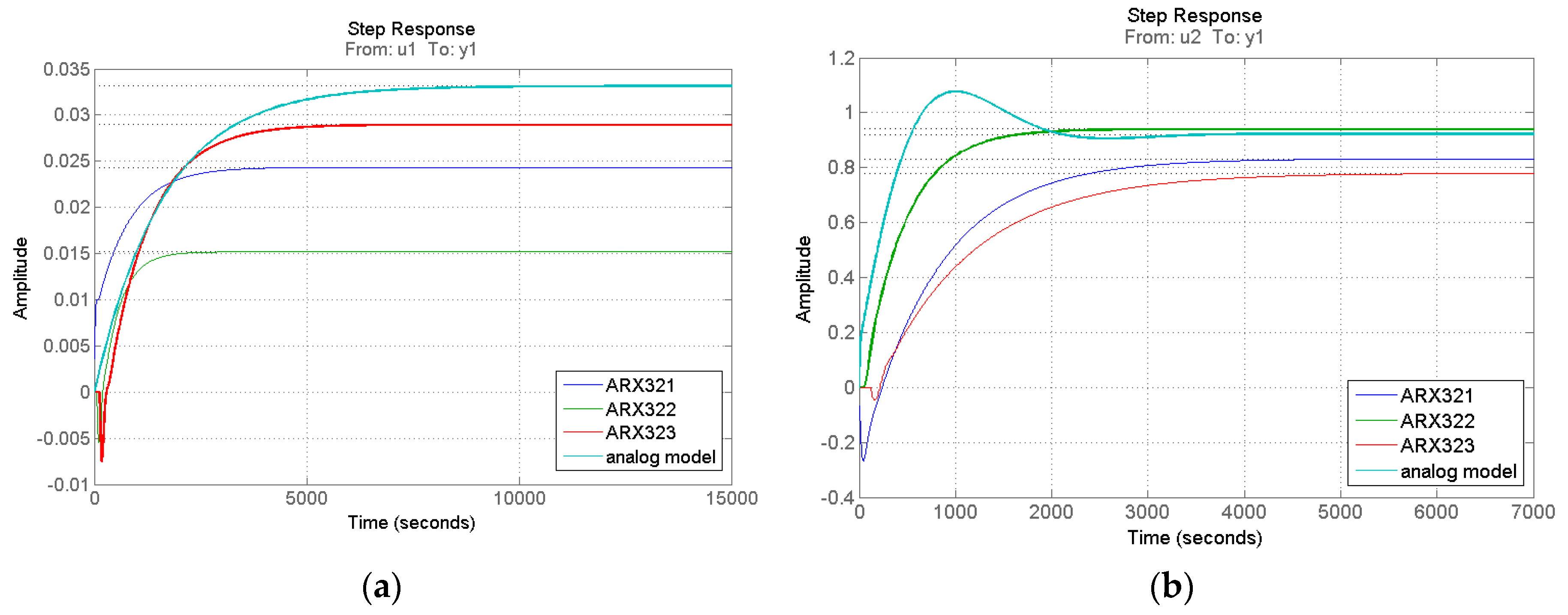
• ARX [3,2,3] for transfer function G1′(s) due to the best matching of step responses curve (Figure 2a) as well as due to the high 90.28% degree of model matching; the delay time of 120 s has been applied (2 measurement steps “backwards”),
• ARX [3,2,2] for transfer function G2′(s) due to the best matching of step responses curve (Figure 2b), as well as due to the highest 92.73% degree of model matching; the delay time of 60 s has been applied (1 measurement step “backwards”) taking into account the calculated time of the working medium flow through the collector from inlet to its outlet.

The curve of the step responses shown in Figure 2a,b are the justification of decisions made. The model ARX [3,2,3] and the step responses determined from the real measurements matches best the step responses of the analog model in the case of transfer function G1(s). The delay time of 120 s (2 steps) has been introduced here. The parametric model of ARX [3,2,2] with the delay of 1 measurement step (60 s), this is the time of the working medium flow through the collector, is the best solution for transfer function G2(s), respectively. The nature of dynamics of the collector is inertial for the transfer function G1(s) of the analog model; and it is a nonminimal phase one for the digital model. According to two separate SISO models in the analog model, there were also two digital models chosen for comparison.

Contrary to the analog model, it is not possible to divide an influence of the input signal on the end temperature in the digital model, as it is created on the real measurements results taken in the online mode. Regardless of the fact if we determine transfer function G1′(s) = T_fout(s)/P(s) or G2′(s) = T_fout(s)/T_fin(s), the other of input signals affects a measurement result. Therefore, step responses of the digital model can differ from the ones presented for the analog model.

The digital model, obtained on the basis of real measurements, does not allow us to conduct simulation tests. For this reason, the next chapter presents simulations of changes in construction and operational parameters on the basis of an analog model.

3. Results

Table 1. Study object construction and operational parameters: basic values.

Construction Parameters
Thickness of glass σs (mm)	4
Thickness of absorber σa (mm)	2
Diameter of flow channels d (mm)	12
Operational Parameters
Working medium flow rate Q (dm3/min)	1.25
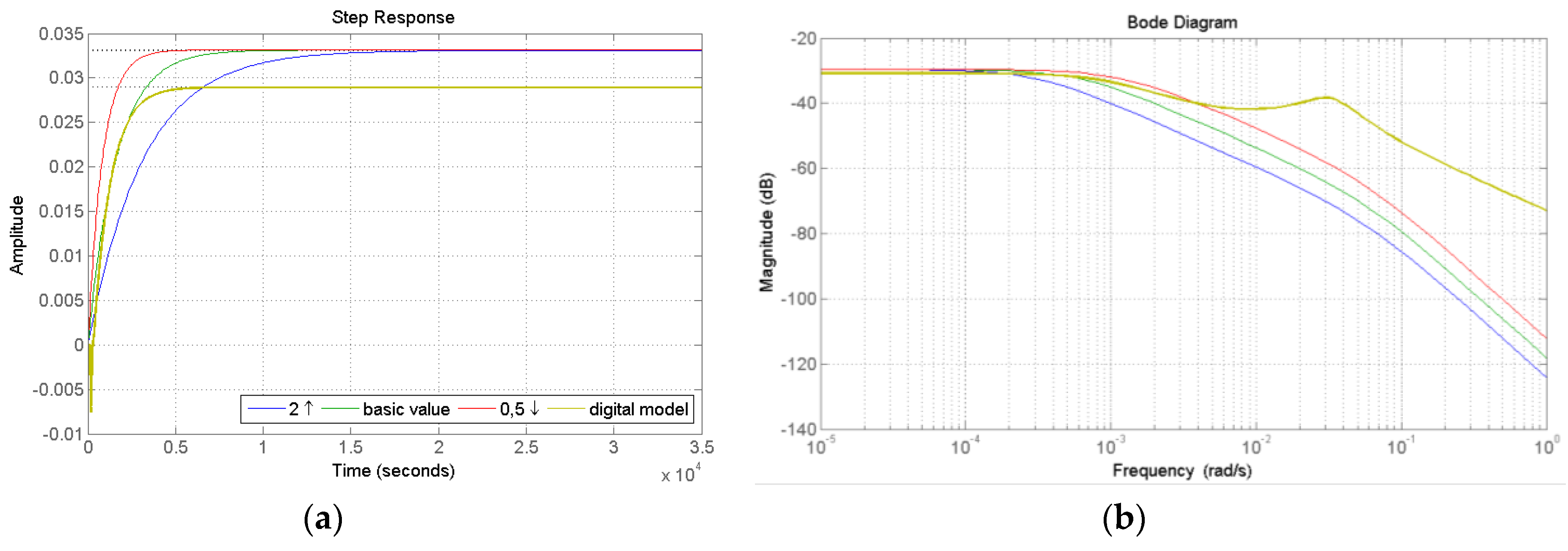
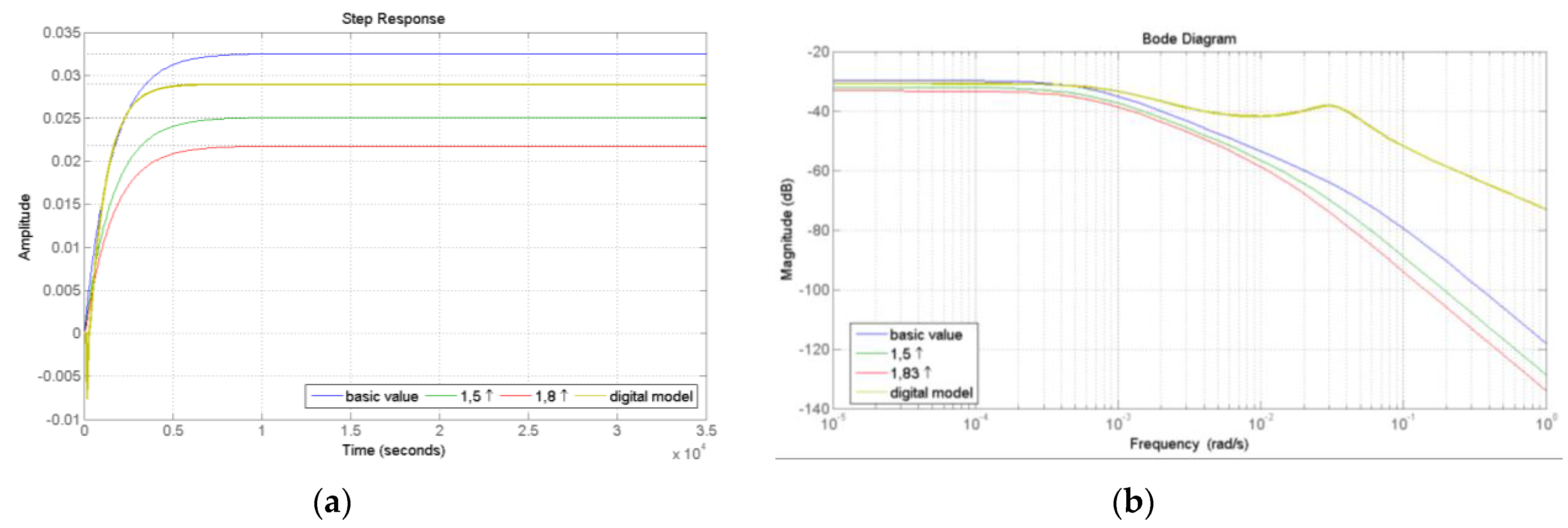
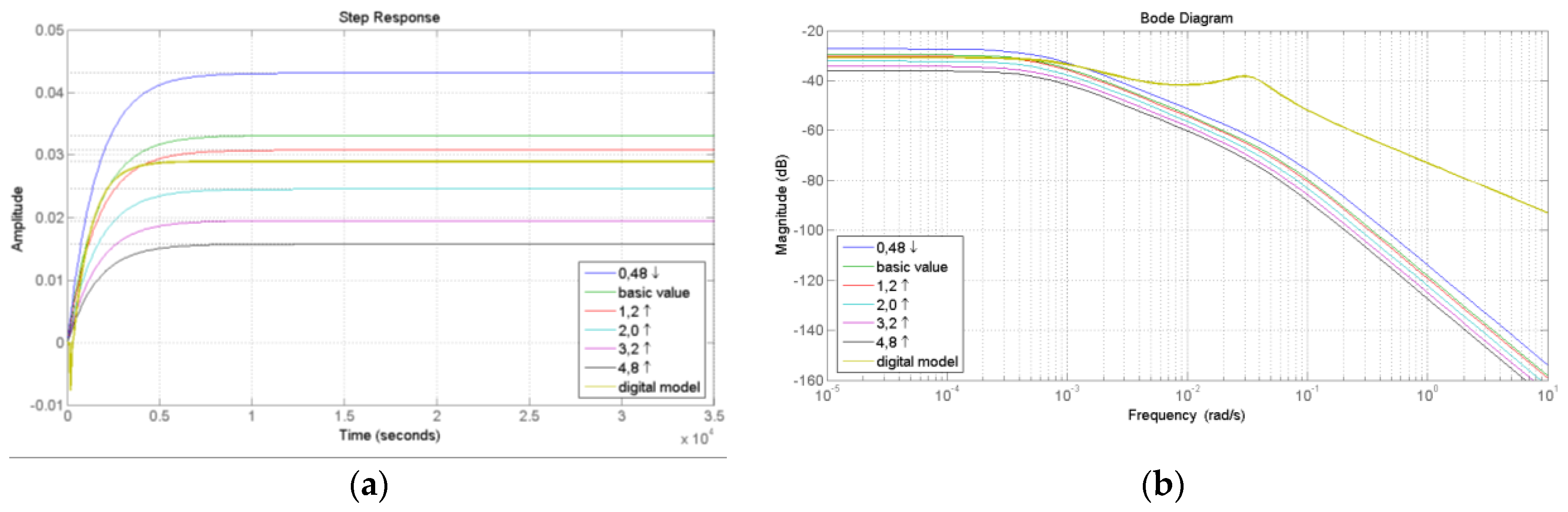
Ambient temperature Ta (°C)	22.5

contains the list of basic values of construction and operational parameters according to investigated solar collector. The diagrams of step response curves show the changes in parameters in relative values related to the parameters of the real collector. The scope of changes in the parameters retains a logical sense. The simulation was performed using the Matlab software.

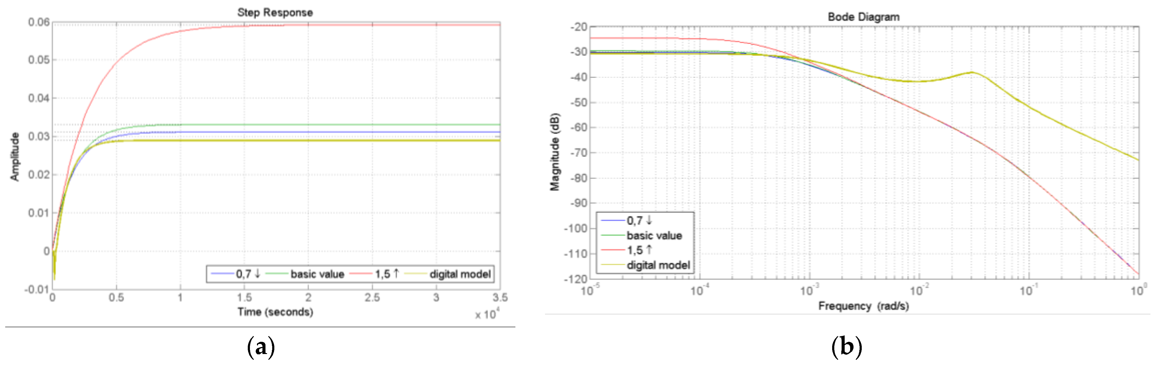
In the case of influence of solar radiation intensity, frequency responses for the particular simulation variants were listed in Figure 3, Figure 4, Figure 5 and Figure 6 below. For both input signals cases, the step responses for the particular simulation variants were listed in Figure 3, Figure 4, Figure 5, Figure 6, Figure 7, Figure 8 and Figure 9 below. On each of the figure, in the legend, changes in the parameters are marked with a down arrow (below the basic value) or up arrow (above the basic value) with a value corresponding to its change i.e., 0.7 with the down arrow is equal to 0.7 times the basic value. The response for the digital model is indicated by the bold yellow line in each of graphs (added to compare, because the analog model is a theoretical one and digital is an experimental one as the result of real measurements). It is the point of reference for the comparison. The differences in the courses of the step and frequency responses caused by the simulation of the construction and operational parameters are the results of changes in the values of resistances (through the change in the heat exchange factors) and heat capacities. These quantities affect in turn the coefficient values of the polynomials of numerator and denominator of the transfer functions, being the quintessence of the collector dynamics.

3.1. Influence of Solar Radiation Intensity

The construction parameters, for which the simulation studies were performed, include thickness of absorber and diameter of flow channels. There were not any significant changes in simulation of the thickness of glass cover. The operational parameters, for which the simulation studies were performed, include working medium flow rate and ambient temperature. Additional calculations for the digital model were made only for operational parameters for three working medium flow values that have taken place. For these flow values, three days for which weather conditions (including daily distribution of solar radiation intensity and a similar total daily dose of solar radiation energy) were similar, were selected from the measurement database. Courses of solar radiation intensity were similar to each other, as well as daily radiation sum. Selection of days with a similar structure (large fluctuations) of temporary changes in solar radiation intensity was made on purpose. For slow changes in solar radiation intensity, the collector responds in a correct way, where the reaction is entirely the result of the effect. The cut-off frequency value indicates how the device suppresses solar radiation intensity fluctuations. With frequency of changes greater than the cut-off frequency, the collector only reacts to a certain mean value of radiation. It does not react to temporary high and low values.

Solar radiation intensity is a variable function of the fundamental component (optimal insolation) and higher harmonic components associated with cloudiness [42]. An analogous change in expenditure (which is generally constant) is not taken into account.

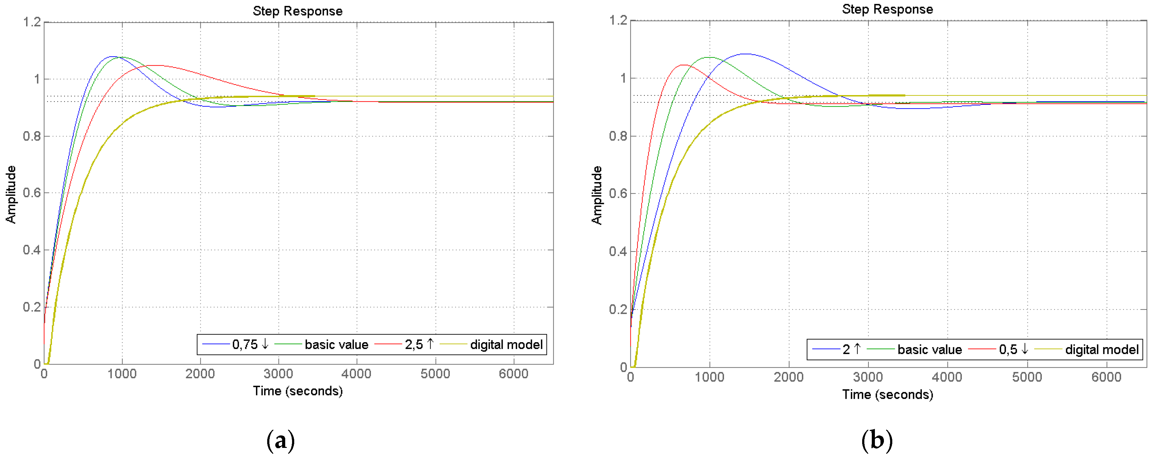
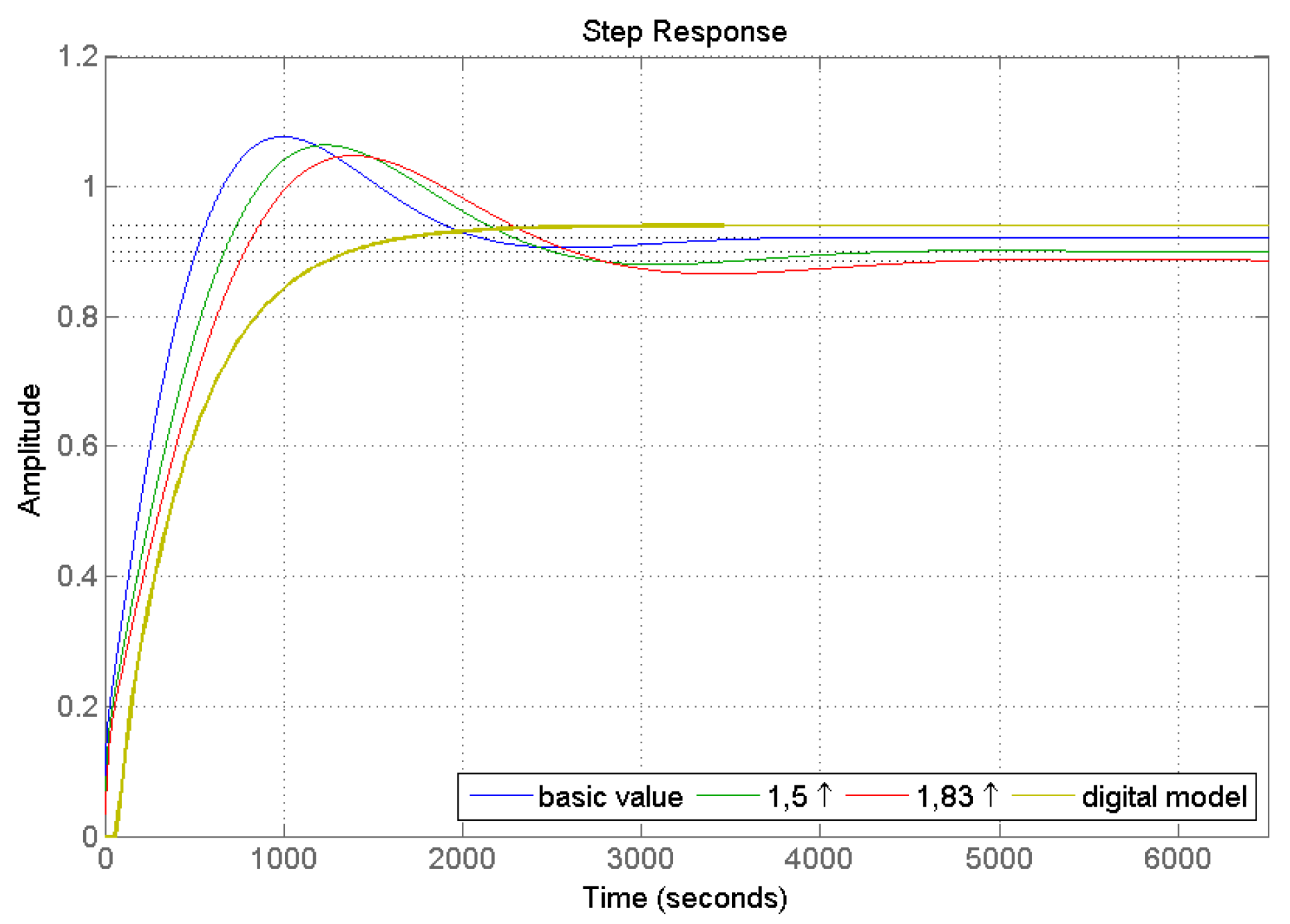
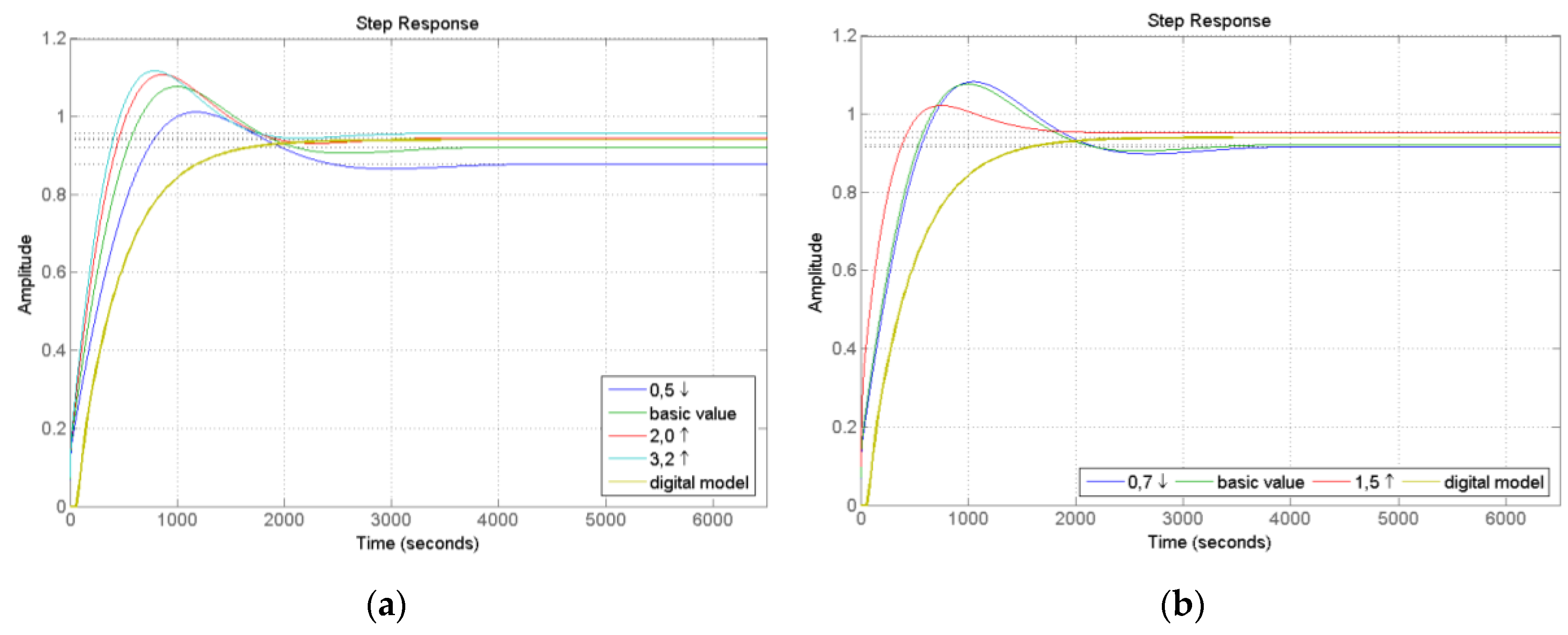
3.2. Influence of Temperature of Working Medium on the Input

The construction parameters, for which the simulation studies were performed, include thickness of glass cover, thickness of absorber, and diameter of flow channels. The operational parameters, for which the simulation studies were performed, include working medium flow rate and ambient temperature.

In the dynamics of heat exchange in the solar collector, for which the step response is determined, interesting phenomena of oscillatory changes appear in the analog model.

4. Discussion

From the step and frequency responses presented in Figure 3, Figure 4, Figure 5, Figure 6, Figure 7, Figure 8 and Figure 9 it results that the second input, on the side of the signal—the temperature at the collector’s input—has the stronger influence on the collector dynamics. For the digital model, this is the nonminimum phase character, i.e., the short-term slight temperature reduction appears first, then the inertial increase of the working medium temperature takes place. For analog model, this phenomenon is more complicated. The step response is of an inertial nature but with initial quickly damping oscillations of small value. The phenomenon is not clear and requires further studies. The other authors pay also attention to this fact in their studies [16,43,44,45,46]. The emerging oscillations on the step responses are related to the G2 segment where

$$G2\left(s\right)=\frac{T_{fout}\left(s\right)}{T_{fin}\left(s\right)}$$

(6)

which is a typical heat exchanger.

The influence of the intensity solar radiation on the working medium temperature rise for both the analog and digital models is not surprising. It is characterized by the inertia. However, for the digital model, inertia is bigger than for analog model. This probably results from the model creation technique. The analog model analyses the influence of the input signals separately, as opposed to the digital model, which cannot separate the influence of the input signals, because it is determined experimentally in the on-line mode.

In case of changes in the thickness of glass cover, the higher influence on the dynamics from the second segment (transfer function G2(s)) is observed. The time constant increases with the increase of the thickness of cover, the temperature oscillations are smaller. In case of the influence of the solar radiation intensity, the insignificant increase of the steady-state level for the thickest glass is observed. However, practically, the thickness of cover does not influence on the signal amplification.

In case of changes in the thickness of absorber, the influence on the dynamics, both on the side of the solar radiation intensity signal (G1) and on the side of the input temperature (G2) is observed. In case of the first segment, the character of the object is not changed, it is inertial. However, the increase of the time constant with the increase of the thickness of absorber is observed. The thicker absorber heats up slower, which is logical. When analyzing the second segment, it is observed (just like for the glass cover) that the time constant increases with the increase of the thickness of absorber and there are slower oscillations. The thinner the absorber, the higher the amplification of the output signal (outlet temperature of working medium). The absorber’s heat energy is acquired better by the working medium because the transfer losses are smaller.

In case of changes in the diameter of flow channels, the flow rate of the working medium is changed. The influence on the dynamics, both on the side of the solar radiation intensity and on the side of the input temperature, is also observed here. In case of the first segment, the inertial character of the object is not changed. The time constant increases with the increase of the diameter of flow channels. In case of the second segment, the increase of the time constant with the increase of the diameter of flow channels is observed as well. The collector achieves the lower level of the steady state for the larger diameters because the flow rate is lower, and the heat transfer coefficient achieves smaller values.

From among operational parameters, the working medium flow rate has the greatest influence on dynamics of the collector operation, which is obviously known in literature. The influence of ambient temperature within the most common range of 15–25 °C is insignificant. If the temperature increases to the values corresponding to the medium temperature at the inlet of the collector, the heat losses decreases and the increase of the temperature level of steady state is evident.

Tests of step responses determined for the analog model indicate that the dynamics of heat exchange in the solar collector depending on two input signals: solar radiation intensity and inlet temperature of the working medium, is varied. In the analog (theoretical) model, it is possible to run simulations with only one input signal, if no changes are assumed for the other. There is no such possibility for the digital model, since it is determined in online mode, for actual parameters, where both solar radiation intensity and inlet temperature change. For step-forcing of input signals of the analog model, in both cases a stable steady state is achieved, but while the first signal interacts inertially on the output signal, the influence of the second one is oscillatory. Oscillations are quickly damped, and their parameters can be affected by such factors as the diameter of the flow channel (construction parameter) or the value of the flow of the working medium. Oscillations in the step response of all devices usually negatively affect work and hinder regulation and adjustment of work parameters. By designing the collector and selecting the appropriate construction parameters it is possible to reduce the occurrence of oscillations during its later operation.

The frequency characteristics make it possible to define the frequency of the input signal changes to which the collector proportionally transfers the changes to the output. Additionally, at what frequencies it suppresses these changes, reacting to certain average values over the time interval.

For step response in the digital model, these oscillations are not apparent, as the first signal (intensity of solar radiation) has a strong inertial effect. All the included charts present comparative characteristics for both models.

The theoretical analog model was built based on thermoelectric analogy. In electrical circuits, in transient states, voltage oscillations occur when there is a connected capacitive and inductive element (capacitor and induction coil). Then, the potential energy accumulated in the capacity C is mutually exchanged into the kinetic energy of the inductance L. Oscillations in the circuit suppressed by resistance R appear. So, if thermoelectric analogy is assumed to be acceptable in modeling thermal phenomena, then the potential energy accumulated in the thermal capacities of the structural components of devices can be converted into kinetic energy of emerging temperature field around these devices; hence the oscillatory nature of the step response determining the impact of the inlet temperature on the outlet temperature of the working medium (similarly as in electrical circuits). Therefore, it seems necessary to consider a solar collector electric diagram that takes this phenomenon into account. It seems necessary to define and introduce to thermoelectric analogy a new physical quantity-thermal inductance.

5. Conclusions

Having the analog model of the solar collector, it is possible to determine the influence of changes in the construction and operational parameters on the dynamics of the appliance operation, thus, to determine design guidelines for solar heating systems. It is not necessary to make prototypes of the appliances or to change the design at the later stage. In addition, it becomes possible to diagnose the solar collector as part of a solar heating system. Using the analog model, it is possible to determine whether a change in the construction and operating parameters has an impact on the time constant, gain factor, or delay time of the analyzed device model.

From among the construction parameters selected for the analysis, the following parameters have the greatest influence on the dynamics of the object: the thickness of absorber and the diameter of flow channels. The thickness of glass cover has definitely a lower influence on the dynamics of the object. When analyzing the diameter of flow channels, the changes in the amplification factor and the slight changes in the time constant values were observed. These studies should be extended by additional analyses in aspects of collector diagnostics. In case of the step responses for the second segment, the oscillating character of the phenomenon was observed. This issue should be developed in further studies. It seems that in modeling heating devices, using a thermoelectric analogy, it is necessary to introduce thermal inductance, which would explain the oscillatory nature of the G2 segment’s influence on the output temperature in the solar collector. Other works have also highlighted this phenomenon [16,45].

In addition to the construction parameters, the operational parameters of the fluid solar collector operation are also an important aspect. While simulating the changes in the operational parameters the scale of their impact on the solar collector operation was shown.

By appropriate selection of the collector’s construction parameters, it is possible to shape the expected course of step responses. It seems possible to obtain an inertial course (attenuation of oscillation) for G2(s) transfer function for a given range of changes in operating parameters.