Article

A Genetic Programming Strategy to Induce Logical Rules for Clinical Data Analysis

by
José A. Castellanos-Garzón
1,2,*,
Yeray Mezquita Martín
1,
José Luis Jaimes Sánchez
3,
Santiago Manuel López García
3 and
Ernesto Costa
2
1
Department of Computer Science and Automatic, Faculty of Sciences, BISITE Research Group, University of Salamanca, Plaza de los Caídos, s/n, 37008 Salamanca, Spain
2
CISUC, Department of Computer Engineering, ECOS Research Group, University of Coimbra, Pólo II - Pinhal de Marrocos, 3030-290 Coimbra, Portugal
3
Instituto Universitario de Estudios de la Ciencia y la Tecnología, University of Salamanca, 37008 Salamanca, Spain
*
Author to whom correspondence should be addressed.
Processes 2020, 8(12), 1565; https://doi.org/10.3390/pr8121565
Submission received: 31 October 2020 / Revised: 18 November 2020 / Accepted: 26 November 2020 / Published: 27 November 2020
(This article belongs to the Special Issue Bioinformatics Applications Based On Machine Learning)

Abstract

:
This paper proposes a machine learning approach dealing with genetic programming to build classifiers through logical rule induction. In this context, we define and test a set of mutation operators across from different clinical datasets to improve the performance of the proposal for each dataset. The use of genetic programming for rule induction has generated interesting results in machine learning problems. Hence, genetic programming represents a flexible and powerful evolutionary technique for automatic generation of classifiers. Since logical rules disclose knowledge from the analyzed data, we use such knowledge to interpret the results and filter the most important features from clinical data as a process of knowledge discovery. The ultimate goal of this proposal is to provide the experts in the data domain with prior knowledge (as a guide) about the structure of the data and the rules found for each class, especially to track dichotomies and inequality. The results reached by our proposal on the involved datasets have been very promising when used in classification tasks and compared with other methods.

1. Introduction

Current data management and storage methods have been challenged by the high increase in the amount of medical data available to us. Obtaining valuable information in the process of knowledge discovery has become problematic. There is an urgent need for new tools and approaches whose mechanism will allow overcoming the present-day limitations of computational medicine, by converting large quantities of data into knowledge. Novel methods will make it possible to go beyond simple data description, providing knowledge in the form of models. Through abstract data models, it is possible to create highly reliable prediction systems [1,2,3,4,5,6,7,8,9,10,11,12,13,14].
The process of knowledge discovery from the data involves, among other techniques, machine learning. Our interest is to select or combine techniques with a high performance in prediction tasks for medical datasets. In medicine, prediction systems are most frequently applied in the field of diagnosis and prognosis. According to previous research on the development of diagnosis systems, it is possible to determine the presence or absence of a disorder through interpretation of patient data [15]. These systems are used specifically in the diagnosis of patients. Prognosis systems use the collected information to predict the progress of the condition a patient is suffering from or to determine whether a patient may suffer a disease in the future. Moreover, they are used to choose the most effective treatment based on the patient’s symptoms and different medical factors [16].
In the context of diagnosis and prognosis, the aim of using intelligent systems based on machine learning techniques is knowledge discovery from the collected information. Sometimes, the discovered knowledge is expressed in a probabilistic model by relating the clinical features of patients to a stage of the target disease. In other cases, a rule-based representation is selected to provide the expert with an explanation of why certain decision was made. Knowledge representations as those described above are known as white box systems and the focus of this research because they express part of the knowledge directly. Finally, there are other cases in which the system is designed as a black box for decision-making, where the system only shows the prediction results. All of these techniques are suitable for making a diagnosis and prognosis of a patient’s condition [17].
Because of all previously explained, this research proposes a system generating classifiers based on genetic programming (GP), which is capable of inducing sets of rules that represent the relationship between the disease and the symptoms experienced by patients. Therefore, our goal is to build a rule-based classifier and compare its ability to correctly classify data with other previously proposed methods. Finally, we analyze the rules obtained by our approach to determine the most important attributes of the dataset. In this case, the system performs a feature filtering process [18,19,20,21]. Rule-based classifiers are an attractive approach since the structure of IF/THEN rules is well-known and can easily be interpreted for knowledge discovery. Hence, such rules not only classify unknown patterns, they also disclose knowledge about the class structure and problem domain. The goal of a rule-based classifier is to find a set of rules that suit a labeled dataset. That is, the discovered rules should represent the target dataset and cover each region of the search space. Hence, the application of GP in the building of rule-based classifiers has been the basis of works such as [22,23,24,25]. Our ultimate goal is to provide the expert with an initial interpretation of the data through our rules-based model that can serve as a starting point in the study of the disease. Hence, we also provide a visual interpretation of the data, which supports the process of knowledge discovery.
In summary, medical databases store a lot of data about the health condition of patients. Such an amount of information is ideal for the application of machine learning techniques, which can transform data into knowledge by analyzing the relationships provided by the model. This mechanism provides a means of hypothesis validation [6,9]. To reach the goals proposed in this work, the rest of this manuscript has been divided into the following sections: Section 2 deals with the background related to this research. Section 3.1 describes the main features of our proposal, encoding, fitness functions, genetic operators and running strategy. Section 4 describes the employed datasets, an analysis of the structure and distribution of the datasets, the experiments to select the best mutation operators for each medical dataset, and accuracy comparison of our approach with other machine learning methods. At the end of this section, an analysis of the rules discovered by the proposal is given and the most influential attributes of the datasets are analyzed. Conclusions, Appendix A (classifiers of our proposal), Appendix B (mutation operator experiments), and the references of this research are the final part of this document.

2. Background

Applications of genetic algorithms (GAs) to analyze medical data have allowed for solving complex problems such as disease screening, diagnosis, treatment planning, pharmacovigilance, prognosis and health care management [26]. GAs have been applied to different fields in medicine, among which we can highlight, Radiology, Oncology, Cardiology, Endocrinology, Pulmonology and Pediatrics, among others. In this context, GAs have been used for edge detection of images obtained from Magnetic Resonance Imaging (MRI), Compute Tomography (CT) and ultrasound [27,28,29]. Making use of these kinds of algorithms, different methods have been proposed to detect microcalcifications in mammograms leading to diagnosing breast cancer [30,31,32]. In other studies, GAs have been used to fuse MRI images with Positron Emission Tomography (PET) in order to generate colored images of breast cancer [33].
In other works [34], a methodology based on the application of a Micro-Genetic Algorithm (MGA) was used to generate the training set that best detects solitary lung nodules. The designed algorithm can detect lung nodules with about 86% sensitivity, 98% specificity, and 97.5% accuracy. In [35], the authors proposed a model using Particle Swarm Optimization method (PSO), a GA and a Support Vector Machine (SVM) in conjunction with feature selection and classification of CT, MRI and ultrasound images. The proposed method was capable of detecting lung cancer with an accuracy of 89.5%.
GAs have also been used to detect patients with some type of carcinoma through Microarray Technology. For example, in [36], a GA combined with an Artificial Bee Colony (ABC) algorithm was proposed. The method aims to make cancer classification in patients through extraction of features from microarray data. This method was tested with a dataset of colon carcinoma, two different datasets of Leukemia, a dataset involving patients with lung carcinoma, and one of patients with Small, Round-Blue Cell Tumors (SRBCT). The method proposed in that paper achieved an accuracy of almost 100% when selecting very few biomarkers.
In the area of Pediatrics, GAs are also being used to detect diseases such as autism from gene expression microarrays. In [37], an approach of GA as a feature selection engine and an SVM as the classifier were proposed to validate the set of features selected. In this work, a performance greater than 86% accuracy for one of the used datasets and a performance of 92.93% accuracy for the other dataset were reached to outperform previous works.
There are other applications of GAs aimed at making predictions from the data acquired from blood tests. In [38], a GA is used to optimize the performance of an Artificial Neural Network (ANN) to detect Coronary Artery Disease (CAD). Through the previous approach, the authors show that CAD can be detected without angiography and consequently eliminate its high cost and the main side effects. In another context, electrocardiogram (ECG) signals in cardiology have been used to detect cardiac arrhythmias [39]. In this work, a method liking a Genetic Algorithm with a Backpropagation Neural Network (GA-BPNN) was proposed to reduce the dimension of the datasets by 50% and achieve 99% accuracy. This makes the method suitable for automatic identification of cardiac arrhythmias.
As stated at the beginning of this section, there are many more applications of GAs to medicine that can be consulted about in the literature [40,41,42]. Since the efficacy of GAs in the medicine field has been proved, we will deal with other recent algorithms (Genetic Programming), which include a GA as its base operation. Genetic Programming (GP) is a kind of GA whose main difference with respect to normal GAs is to produce expressions (functions or programs) as outputs rather than data [43,44,45]. An example of the use of this kind of algorithms in the medical field is shown in [46]. In this work, a GP algorithm is proposed to automatically create the best mathematical formula that combines a set of preselected features from a Magnetoencephalography (MEG) dataset. To evaluate the generated formulas, a K-nearest neighbor algorithm (KNN) is used. This approach achieved 91.75% sensitivity and 92.99% specificity in the diagnosis of Epilepsy.
GP is also used to provide diagnosis from MRI images by evaluating the medical spine condition of patients [47]. The GP algorithm proposed in this work uses of a fitness function based on expert knowledge, in this case, a neuroradiologist. The rules rendered in each generation of the algorithm are evaluated and then compared with the true results in order to select the rules with less difference. The  accuracy reached was greater than 90% in the conditions evaluated by combining the GP algorithm and expert knowledge.
Another example of GP applied to medicine is image classification [48]. In this work, a GP algorithm is proposed to create and evolve tree-based classifiers, whose aim is to diagnose active tuberculosis from raw X-ray images. The framework proposed was able to achieve a competitive classification and a superior speed compared to methods that rely upon image processing and feature extraction.
In general terms, GP represents a flexible and powerful evolutionary technique that uses a set of functions and terminals to produce computable expressions. Hence, this research presents a GP method to render rule-based classifiers for knowledge discovery from medical data. Some of the advantages related to this kind of classifiers generating comprehensible knowledge are high expressiveness, which allows them to render models that are very easy to interpret. Such rules can be altered to handle missing values and noise from attributes of the data set. They are relatively easy to obtain and very fast at classifying new patterns (or data) [49]. Moreover, a very important advantage of such rules for machine learning is that they are intuitively comprehensible to the user [50,51]. Another advantage related to the above is that they are not only used to classify, but they also represent, by themselves, a process of knowledge discovery, providing the user with new insights into the data and their application domain  [52].

3. Materials and Methods

3.1. Evolutionary Strategy to Build Rule-Based Classifiers (ESRBC)

This section presents our main proposal, the evolutionary method (ESRBC) to render rule-based classifiers. Thus, we describe the strategy to follow by ESRBC, individuals, crossover, mutation operators and fitness functions. Individuals represent logical rules adopting an internal representation of a linear sequence of clauses (or comparisons) separated by conjunctions AND. Individuals to be built in this proposal follow the Michigan-style [24,50,53,54]; hence, each individual encodes a single rule (with a linear chromosome) with a variable length, where each rule is associated with the class of the dataset it represents. Therefore, an individual can be evaluated as True or False according to the pattern evaluated in the antecedent of the rule. As applicable, the pattern may or may not belong to the class assigned to the rule.
As explained, the individuals generated by ESRBC represent logical rules of type I F < C L A U S E S > T H E N < C L A S S > , where < C L A U S E S > is formed by a set of clauses (or comparisons) separated by conjunctions AND. < C L A S S > is the class of the dataset that is being represented by the rule or, in other words, the class to which the rule belongs. A more detailed representation of a rule can be given as follows:
I F ( a t 1 o 1 v a l 1 ) A N D ( a t 2 o 2 v a l 2 ) A N D A N D ( a t n o n v a l n ) T H E N c l a s s = k ,
where ( a t i o i v a l i ) is clause number i, a t i is an attribute of the dataset, o i is a comparison operator from set { < , > , , , = , } , v a l i a value of the set of all possible values admitted by a t i , whereas k is the class of the dataset covered by the rule. An example of logical rules representing a dataset with attributes { p , q , r , s , t } and two classes { 0 , 1 } can be as follows:
I F ( p > 12.3 ) A N D ( p 15 ) A N D ( s 3.4 ) T H E N c l a s s = 0 ,
I F ( p 12.3 ) A N D ( r > 7.4 ) A N D ( t 2 ) T H E N c l a s s = 1 ,
which means that, if there is a specific pattern ( p i , q i , r i , s i , t i ) from the domain of the dataset, whose values p i and s i hold the antecedent of the rule in class-0, then such a pattern belongs to class-0. Likewise, if attribute values p i , r i , t i hold the antecedent of the rule in class-1, then this pattern is in class-1. Keep in mind that the challenge that each rule learned from a dataset must meet is generalization. In other words, the set of rules holding a dataset should generalize enough in such a way that the pattern space be properly partitioned. Thereby, each region of the space is covered as much as possible by the set of rules.
Continuing with the description of the rule concept, we define the length of a rule as the number of clauses that form it. The evolutionary algorithm (EA) of our approach, which is responsible for the search process for a diverse set of rules, adopts the sequential covering strategy for each class of a dataset [51]. Sequential covering is a technique that discovers one rule at a time. The EA is executed multiple times to build a complete set of rules representing each class of a dataset. During each execution, the best rule evolved through the EA is added to the set of previously discovered rules and the patterns covered by this rule are removed from the dataset. The process is repeated until there are no more patterns to be covered. The steps followed by this methodology can be described as follows:
  • Select the set of patterns from a new class i in the input dataset;
  • Create an initial population P 0 of rules candidate to represent patterns in class i;
  • Run the EA on P 0 to achieve a final population P f ;
  • Add the most fit individual (rule) r of P f to the set of rules R (R is empty initially);
  • Remove all patterns from class i holding rule r;
  • If class i is not empty, then go to step 2;
  • If there are more classes in the dataset, then i : = i + 1 and go to step 1;
  • At the end of the process, R has a set of rules learned from each class of the input dataset.

3.2. Fitness Functions

This section introduces the fitness functions used in the evolutionary algorithm of our approach. In this case, the fitness functions defined are based on the concept of accuracy [52,55,56]. The accuracy of a rule is the fraction of patterns from its class, covered by the rule. Then, according to the definition above, we are going to introduce two variants of fitness functions based on accuracy. However, we firstly need to define two functions which evaluate a pattern e in a rule r. Then, the first function is g acting on r and e, i.e., g ( r , e ) , which computes the number of clauses of r evaluated True when e is evaluated in r. The second function defines the evaluation of a pattern e in r ( r ( e ) ) in the following way:
r ( e ) = 1 , if e belongs to the class of r , in this case we say , e holds r ; 0 , otherwise .
Note that g ( r , e ) evaluates the number of clauses in r holding a pattern e, whereas r ( e ) evaluates the rule to 1 (True) if it covers pattern e (all its clauses become True). Additionally, if we want to specify the class of both r and e, we write r i and e i respectively, where i is a class of the dataset. Finally, the two expected fitness functions are given below. For this case, both fitness functions define a maximization problem. The first objective of f 1 assesses accuracy based on the number of clauses turned true by patterns of the target class, whereas the second objective acts as a penalty for patterns not belonging to the class of the rule, whose values make the clauses of the rule true. The same situation happens for f 2 , but, in this case, the accuracy is assessed by considering the number of patterns holding a rule r. f 1 has been created to be run in the first generations of the evolutionary algorithm where rules have randomly been created and no pattern holds them. However, the use of f 2 makes more sense in a second stage of the evolutionary algorithm (after applying f 1 ) when the rendered rules have reached a certain learning level.
Definition 1.
Fitness function- f 1 .
If D is a labeled dataset with k classes, C i a class of D and r i a rule of C i and consider i , j [ 0 , 1 , , k 1 ] . Then, we define a fitness function- f 1 applied to r i as:
f 1 ( r i ) = 1 | C i | · | r i | e C i g ( r i , e ) 1 | D | | C i | e C j , j i g ( r i , e ) + 3 .
Definition 2.
Fitness function- f 2 .
From the same conditions given in Definition 1, we define fitness function- f 2 applied to a rule r i as:
f 2 ( r i ) = 1 | C i | e C i r i ( e ) 1 | D | | C i | e C j , j i r i ( e ) + 3 .
Both fitness functions have been focused on a maximum problem: the bigger their values, the more fit the evaluated rules. In the first fitness function, the first objective deals with a kind of accuracy using g, which consists of computing the number of clauses evaluated True in the current rule for all pattern of its class. The second objective measures the number of clauses evaluated True by the current rule for all pattern belonging a different class of the rule class. This fitness function is useful in the evaluation of rules built in the first generations of the EA, where the rule accuracy is zero. The second fitness function is responsible for measuring the number of patterns from the rule class holding the rule versus the number of patterns of other classes holding the rule.

3.3. Genetic Operators

The crossover operator used in this method to recombine clauses from two parent-rules to achieve two new children-rules performs as the classical operator [57]. That is, the crossover operator selects a random position (with a uniform distribution) from two parent-rules and exchanges two segments of clauses from them to achieve two children, inheriting part of the clauses (genetic code) of their parents. In other words, given two rules, the position of a clause is randomly selected. Then, the clauses located on the right or left side of both rules (which is also decided at random) are exchanged to create two new rules. The mutation operator is responsible for providing new information to the individuals generated. In this case, we provide three types of mutation operations by defining a mutation group for each one:
  • Mutation by clause, M1: Changes the attribute, comparison operator or value in a randomly chosen clause from the rule by others, also randomly selected;
  • Mutation clause by clause, M2: This operator applies the M1 operator clause by clause to a rule. For each clause, the operator decides whether to mutate. If a mutation has been selected, then the operator decides what mutation type to perform. Namely, changing the attribute, the comparison operator or the value of the attribute in the current clause.
  • Mutation by transformation, M3: This operator can remove a part of the rule, add a new rule, or apply the M1 operator to the rule. One of the three operations above is selected at random. In the first operation, a position in the rule is randomly selected to remove the left or right side. Then, it randomly selects the part of the rule to be removed. The second operation adds a new rule at the end of the current rule. The added rule is randomly created (by also choosing its size in a random way).
The mutation operator applied to each mutation in the rules is selected at random. Note also that the goal of defining the M2 and M3 compound mutation operators is to create different mutation levels from the M1 basic mutation operator. This allows us to explore different alterations on the individuals yielded from generation to generation. Each of these operators (M1, M2, and M3) performs an alteration level of individuals by regarding a minor (M1), medium (M2) and higher level (M3) of alteration.

3.4. Running the Evolutionary Algorithm

Once the genetic operators have been defined, the evolutionary algorithm (EA) of our proposal ESRBC is responsible for discovering each rule covering different parts of the search space, hoping the rules can generalize. Hence, the EA is run following the general scheme given by evolutionary algorithms [57,58], with the particularity of introducing an elitism which is transmitted from generation to generation and tournament selection as the adopted selection method.
Aside from the above, the EA includes an evolutionary strategy of local search (Algorithm 1 ESLS), which acts on the population or the most fit individual returned by the EA. In fact, the option of executing Algorithm 1 from a population or a single individual is a parameter of the algorithm. The term local search is because Algorithm 1 is based on mutation operators and in each generation, Algorithm 1 replaces only individuals who have improved their value fitness after the mating process. The goal of this strategy is to refine the solutions of the EA by making an in-depth search. Hopefully, the individuals from the EA are close enough to a global optimum. Therefore, Algorithm 1 is in charge of searching such an optimum. This idea has been taken from [59] and implemented in [60] with good results. The idea is as follows:
  • Running a genetic algorithm (GA) until it slows down, then letting a local optimizer take over the last generation (and/or best individual) of the GA. Hopefully, the GA is very close to the global optimal.
ESLS has been defined below. This strategy improves a population of individuals or a single individual given by ESRBC. Finally, both ESRBC and Algorithm 1 were implemented in the C++ programming language, whereas the experiments were performed under R-Project [61].
Algorithm 1 ESLS
Input: POP, the population composed by the individuals in the last generation of the EA. MaxGeneration, the number of generations. MO applies one of the mutation operators given in Section 3.3, chosen at random. f 2 , fitness function given in Section 3.2.
Output: POP, as a result of improvement of the input.
1. t : = 0 ;
2.while t < MaxGeneration do
3.  t : = t + 1 ;
4. for all rule r in POP do
5.  % Computing fitness
6.  f := f 2 (r);
7.  % Applying mutation.
8.  newr := MO(r);
9.  % Evaluating new individual.
10.  newf := f 2 (newr);
11.  % Updating the improved individual.
12.  if newf > f then r := newr;
13. end for
14.end while
15.end.

4. Results

This section describes the experiments carried out by our proposal on the clinical datasets, which have been selected from Machine Learning Repository [62]. The used datasets deal with Heart, Hepatitis, and Dermatology diseases, which we call DS1, DS2, and DS3, respectively, and have the features listed below. Note that Number of patterns refers to the number of instances (number of rows) of the dataset while Number of attributes refers to the number of variables (number of columns) of the dataset.
  • Title: SPECTF Heart Dataset (DS1);
    • Number of patterns: 267;
    • Number of attributes: 22 plus the class attribute;
    • Number of classes: 2 classes;
    • Attribute type: binary;
    • Missing attribute values: No missing values.
  • Title: Hepatitis Domain (DS2);
    • Number of patterns: 155;
    • Number of attributes: 19 plus the class attribute;
    • Number of classes: 2 classes;
    • Attribute type: Categorical, Integer and Real;
    • Missing attribute values: yes (10-nearest neighbor technique was used in this research for imputation of missing values).
  • Title: Dermatology Database (DS3);
    • Number of patterns: 366;
    • Number of attributes: 34 plus the class attribute;
    • Number of classes: 6 classes;
    • Attribute type: Categorical and Integer;
    • Missing attribute values: yes (20-nearest neighbor technique was used in this research for imputation of missing values).

4.1. Exploring and Analyzing the Datasets

This section shows different linked views of the distribution and structure of the datasets, which allow us to have an initial assessment of their behavior. This can also help explain some of the results obtained for the methods applied. Starting with the DS1 dataset shown in Figure 1, we have that this dataset is represented by a diamond-shaped cloud of points. According to the point distribution in each class, Class-1 is much more compact and bigger than Class-0. Therefore, Class-0 could need more rules to classify the patterns of its class than Class-1. Since points in Class-1 are more scattered in space and both classes are intertwined, it would be more difficult for this class to find rules that do not classify patterns in Class-0 by mistake. On the other hand, at the bottom of the figure, there is the heatmap of the dataset where both classes are separated by boxes. Note that the values in this dataset are binary and, in Class-0, values 0 predominate while, in the other class, values 1 predominate. This means that, unlike Class-1, Class-0 is characterized by the absence of the property denoted by many of the attributes evaluated by the disease represented in the dataset.
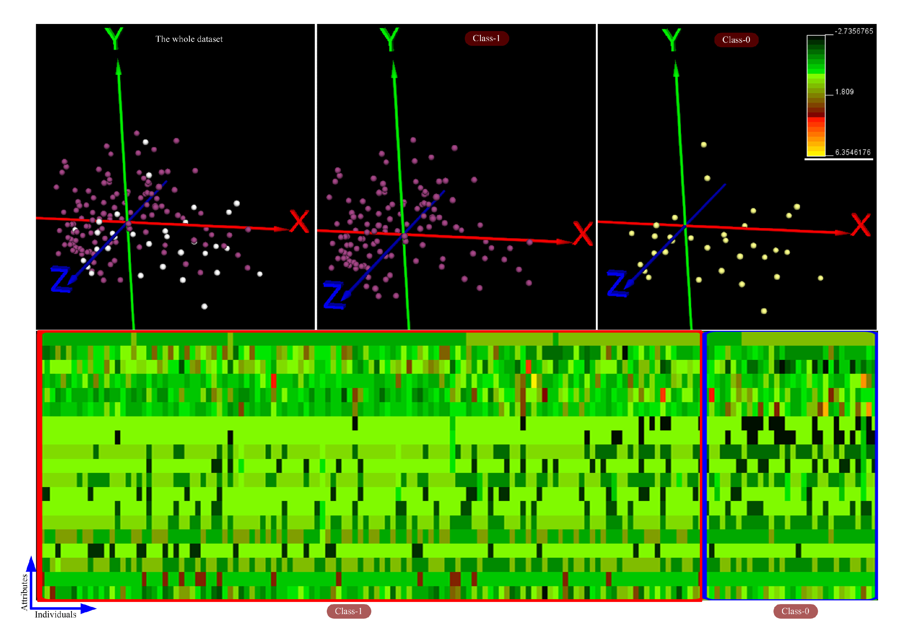
Turning now to the DS2 dataset shown in Figure 2, we have that this dataset is represented by a cloud of points in tree form at the top of the figure. As in the DS1 dataset, both classes are intertwined, Class-1 is more compact and bigger than Class-0. Unlike the DS1 dataset, points are more scattered in space, which can induce a smaller number of rules classifying each class. Note that it is more difficult to find visual differences separating both classes for the heatmap given for DS2 than for the case of DS1. The above can imply that DS2 is a difficult dataset to classify, which tests any applied classifier (method).
As for the DS3 dataset shown in Figure 3, we have that, unlike the other datasets, this one has six classes, which may increase the classification error of the methods applied to the dataset. The point cloud of this dataset, shown at the top of the figure, is T-shaped with agglomerations of points at the ends and in the center of the 3D-scatterplot. Note that the same T-structure of the dataset is maintained for the points in each class. In this case, each class may generate four rules since there are four clusters in each class. However, the greatest difficulty would be to separate the classes from the others, since the six classes are very interrelated. Finally, note that classes 0, 1, and 2 differ from classes 3, 4, and 5 in that, in the latter, the light green color predominates (values below the average value of the whole dataset), while, in the rest of classes, the representative color is brown (values above the average value of the whole dataset). This shows that classes 0, 1, and 2 share some type of similarity with the type of disease represented by each class, which makes the difference from the diseases represented in classes 3, 4, and 5. The same reasoning done for classes 0, 1, and 2 is met for classes 3, 4, and 5 of DS3.

4.2. Mutation Operator Evaluation

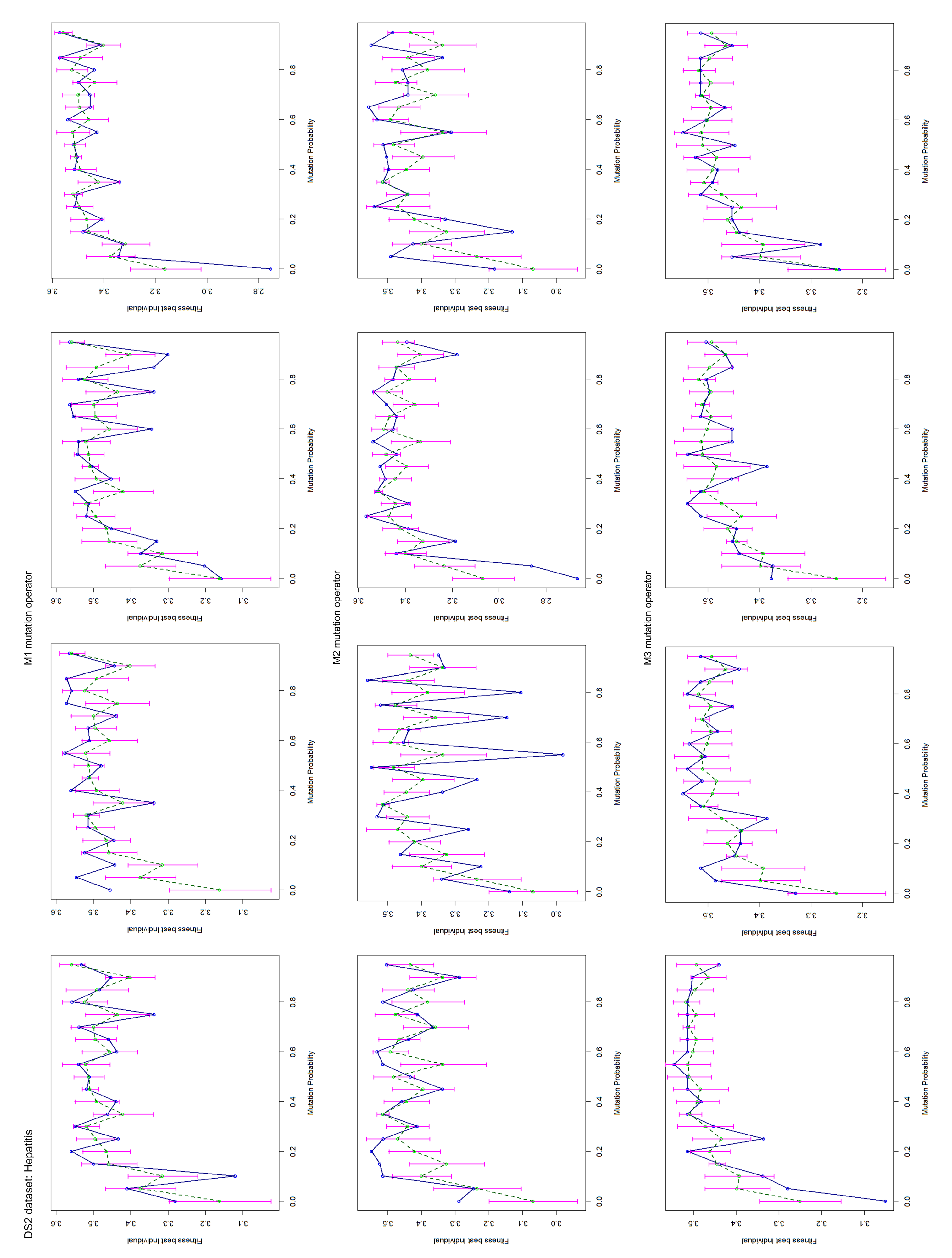
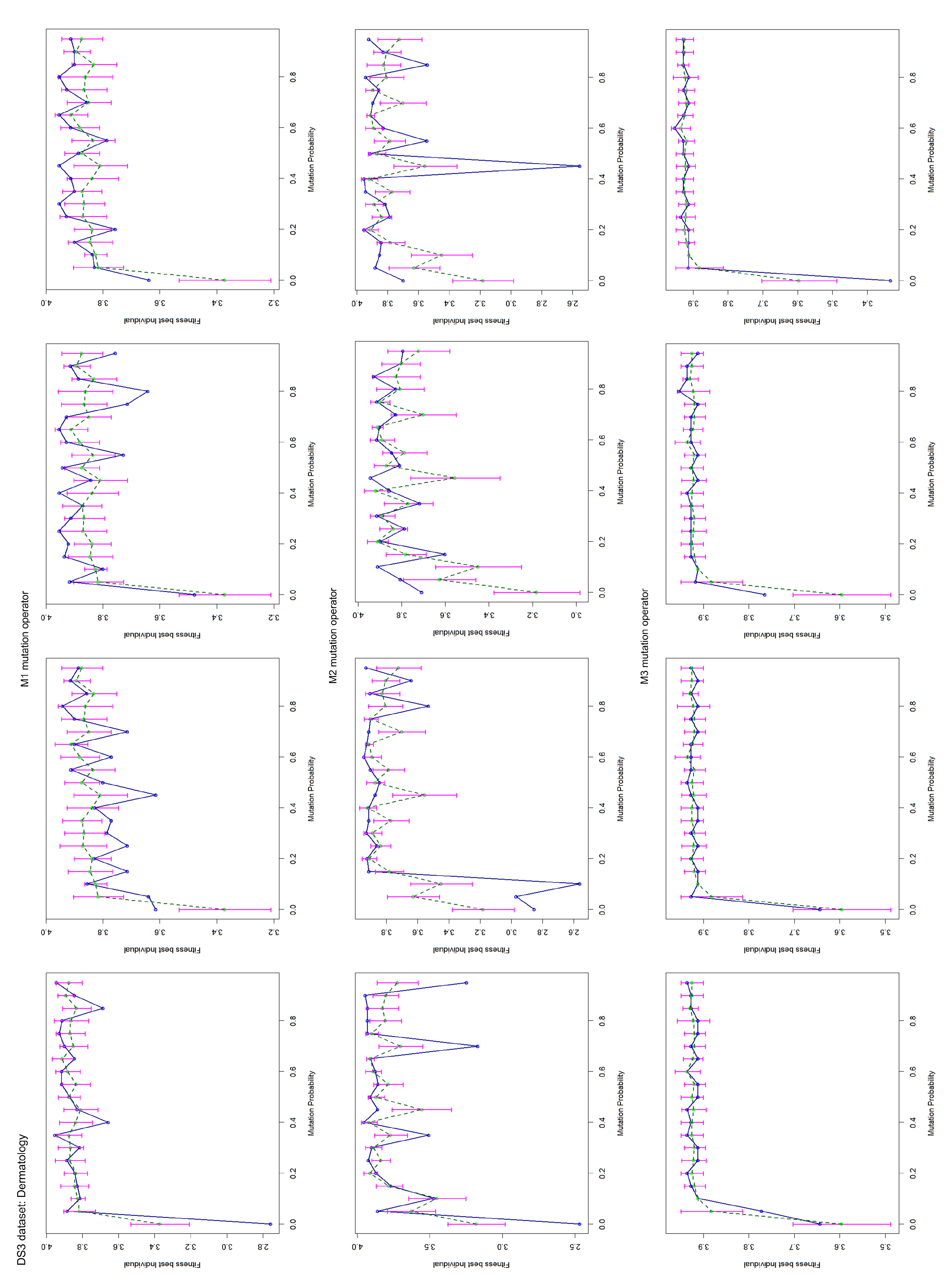
This section deals with the evaluation of mutation operators M1, M2, and M3 from their effectiveness and behavior under the different given datasets. The goal of this test is to carry out an analysis of the behavior of the mutation operators to select the operators having a better performance on a given dataset. Consequently, we have run the evolutionary method (ESRBC) using only the mutation operators (without the crossover operator). Then, ESRBC is run 20 times for each operator and each dataset (DS1, DS2, and DS3) in the following way: for each mutation operator applied to a dataset, ESRBC has been run 20 times, each using a different mutation probability value. In each execution, the probability value is increased in a step of 0.05 , starting from 0. Then, for each mutation value, the fitness value of the most fit individual in 5000 generations has been taken out to render the graphics given in Figure A1, Figure A2 and Figure A3 (Appendix B) for datasets DS1, DS2, and DS3, respectively. Thus, the  achieved graphics represent mutation probability values in x-axis versus fitness value (y-axis) for the best individual yielded in each mutation probability value.
As shown in these figures, each row deals with four graphics, which correspond to the same experiment repeated with the same mutation operator. Since ESRBC includes a stochastic process in the search, we have repeated the experiment four times for each mutation operator. Therefore, each row in these figures correspond to a mutation operator, i.e., the first row represents M1, the second and third rows correspond to M2 and M3, respectively. Finally, each graphic in each row represents the fitness values reached by the best individuals for the current operator mutation. Such values are represented by means of a blue curve. The mean fitness values from the four experiments carried out (in each row) for each operator are represented through the green curve, whereas the standard error bars are stressed in pink lines.
By making now an analysis of the results for these three figures, we can say that, for the DS1 dataset, the results in Figure A1 (Appendix B) show that, for operators M1 and M2, most of the reached fitness values (blue curve) are between 3 and 3.4 . On the other hand, there is overlap between the error bars (pink bars), which indicates uniformity of fitness values for M1 and M2 with respect to different mutation probability values. However, the fitness values (blue curve) given in the graphics for operators M1 and M2 present more oscillations than the ones represented by the curves given for the M3 operator. In addition, the standard error bars for the M3 operator are smaller, indicating that the average value plotted is more reliable than the one of those in M1 and M2. Moreover, most fitness values with respect to mutation probability values are between 3.2 and 3.4 . Thus, the M3 operator appears to be more significant for the DS1 dataset than operators M1 and M2. Hence, we can use only M3 as the mutation operator when using the evolutionary method to build a classifier on the DS1 dataset. In addition, keep in mind that, since the standard error bars overlap in the M3 operator, it is not necessary to assign a big valor of mutation probability in the running of ESRBC to build the rule-based classifier. The above improves the runtime of the method.
Unlike Figure A1 (Appendix B), graphics in Figure A2 present more oscillations according to the curve representing fitness values across from mutation probability values (blue curve). However, the error bars maintain an overlap. In addition, note that the fitness values achieved for M1 and M3 are higher than those given in Figure A1. That is, for M1, most fitness values are between 3.4 and 3.6 . For M3, most fitness values are between 3.5 and 4 whereas fitness values for the M2 mutation operator are more unstable with respect to mutation probability values. Therefore, we can use operators M1 and M3 as the only ESRBC mutation operators when using the DS2 dataset.
For the results obtained from the DS3 dataset, Figure A3 (Appendix B), we have that they are like those given in Figure A1. Hence, by applying the same reasoning as the one given in Figure A1, the M3 mutation operator is the most stable and so the operator that best performs on the DS3 dataset. Once the mutation operators performing well on each dataset have been chosen, we can proceed to compare the classifiers induced by our method with other machine learning methods under the accuracy measure.

4.3. Accuracy and Comparison of the Evolutionary Method

The accuracy of the rule-based classifier yielded by our approach has been computed and compared with other methods for each introduced dataset. A stratified 10-fold cross-validation was used to measure the accuracy of all methods. The evolutionary method (ESRBC) defined was run in two stages. In the first stage, ESRBC was run by using the f 1 fitness function, whereas f 2 was used in second stage. The settings of ESRBC for each dataset have been listed in Table 1 and the methods used in the comparison process [55,56,63,64] have been listed in Table 2. Then, the results reached by ESRBC compared with other methods have been listed in Table 3. The best accuracy value for each dataset has been underlined. ESRBC reached the best values for the DS1 and DS3 datasets while its accuracy for DS2 was not very different from the one of the method reaching the best value. Since the number of patterns for the classes of the DS1 and DS2 datasets are unbalanced, Table 3 also shows the Youden index which deals with unbalanced classes in a dataset. This index is defined as s e n s i t i v i t y + s p e c i f i c i t y 1 .
Note that the methods listed for the DS3 dataset are different from those used in DS1 and DS2. This is because the methods used for DS1 and DS2 are for binary classification, whereas the DS3 dataset has six classes. Therefore, we need to use multiclass methods in DS3, different from the methods used in the previous datasets. On the other hand, the greatest accuracy reached for the DS1 and DS2 datasets was less than 90%, which tells us that they are difficult to classify (due to their compactness and difference in the size of their classes), as explained in Section 4.1. However, the greatest accuracy reached for the DS3 dataset was greater than 90%, although DS3 has six classes. This may be due to the distribution of the dataset, where each class is represented by four groups of points separated from each other (which facilitates the classification), as explained in Section 4.1.

5. Discussion: Rule Analysis

This section makes an analysis of rules discovered by the classifiers induced by the evolutionary method (ESRBC) for each dataset in Table 3. The aim of this analysis is to discover knowledge from those rules and identify attributes and relations relevant for the disease. In that sense, such prior knowledge would act as a starting point for experts in this field.
Appendix A lists the rules given by the best classifier found by our proposal for each dataset. The analysis carried out in this section is based on knowledge disclosed from such rules. Starting from the DS1 dataset, we have that it contains diagnoses based on 22 features, built from Single Proton Emission Computed Tomography (SPECT) images, which aim to distinguish between heart disease and normal heart operation. For this case, ESRBC found six rules for a class and only one rule for the other class. Of the 22 attributes, only five of them were not used by any rule (F1, F2, F9, F12, and F18), which implies that they are not important in the classification of the disease and may be discarded from the analysis. However, attributes F5, F21, and F22 achieved the greatest frequency of occurrence by rules in class-0 (they occurred in 42.86 % of rules). Hence, such attributes are representative for class-0. Meanwhile, class-1 used a single rule with only one attribute, F8. The F8 attribute has been used in both classes, so it is not only important for class-1 but also for the disease in question.
The DS2 dataset consists of 19 attributes and two different classes, including clinical and biochemical variables. ESRBC found three rules for class-0 and 2 rules for class-1. Of the 19 attributes, 12 of them were used in the rules and seven of them were not used by any rule (STEROID, MALAISE, ANOREXIA, LIVERBIG, LIVERFIRM, VARICES and HISTOLOGY). Thus, they can be discarded from the classification process. In addition, the most frequent attributes by rules in class-0 were ALBUMIN with 100 % , PROTIME, AGE and ALK PHOSPHATE with 66.67 % , whereas class-1 only used the ALBUMIN and SEX attributes. Note that the ALBUMIN attribute is the only one used in both classes. Therefore, this attribute is significant for the study of the disease. This way, we can identify three groups of patients presenting different features in class-0: patients holding { A L B U M I N 3.99 , P R O T I M E 50 , S E X = 1 } , patients holding { A L B U M I N 3.80 , A G E 37 , 64.88 A L K P H O S P H A T E < 95 } and patients holding { A L B U M I N 3.50 , P R O T I M E 56.16 , A L K P H O S P H A T E > 104.77 , A G E 30 } . Patients in class-1 are government by attributes { A L B U M I N 2.9 , S E X = 2 } .
The DS3 dataset presents data of patients of six different erythemato-squamous diseases. That is, psoriasis, seboreic dermatitis, lichen planus, pityriasis rosea, cronic dermatitis and pityriasis rubra pilaris. The main interest of applying our proposal to this dataset is that these diseases are difficult to distinguish, and they normally require a biopsy and present many common histologic characteristics. The classifier found for DS3 rendered 11 rules distributed in the six classes. Namely, 1 rule in classes 0, 2, 4 and 5; 2 rules in class-1 and 4 rules in class-3, which coincides with that explained in Section 4.1 for DS3. Of the 33 attributes in this dataset, 12 were filtered by the rules of the classifier, whereas 21 were not selected by the same rules. In this case, note that a significant number of attributes was not chosen by the rules of the classifier. This means that the classifier was able to filter the most relevant features (12 features, see Appendix A.3) for the diseases represented by DS3, whereas the remaining features can be removed from the analysis, since they do not provide valuable information.
By analyzing the attributes in this dataset, we have that the FIBROSIS, AGE, ITCHING, and SPONGIO attributes have the greatest frequency of occurrence. In particular, FIBROSIS appears in 50 % of the classes of this dataset (classes: psoriasis, seboreic dermatitis and cronic dermatitis), whereas AGE appears in 80 % of rules in class-3 (lichen planus), ITCHING, and SPONGIO appear in 60 % of rules in the same class-3. In particular, patients in each class are governed by the following relationships:
Class-0: 
patients holding { F I B R O S I S = 0 , S P O N G I O = 0 , E L O N G A T I O N > 0 } ;
Class-1: 
patients holding { F I B R O S I S = 0 , A G E = 20 , D B O R D E R S 2 } ;
Class-2: 
patients holding { B A N D L I K E > 1 , T H I N N I N G 1 } ;
Class-3: 
this class supports four age-related subgroups of patients, namely, { A G E 18 , I T C H I N G 1 } , { A G E = 27 , I T C H I N G < 2 , S P O N G I O > 0 } , { A G E = 36 , I T C H I N G 1 , S P O N G I O > 0 } and { A G E = 62 , S P O N G I O > 0 } ;
Class-4: 
patients holding { F I B R O S I S > 0 , P O L Y P A P U L E S = 0 } ;
Class-5: 
patients holding { P E R I F O L L I > 0 , F O L L I P A P U L E S > 0 } .
Note that, unlike the AGE feature, a value zero for the remaining features means that such a feature is not present in the patient, whereas a value greater than zero means that the patient presents the feature to a degree associated with the value. Consequently, with the results above, we can say that the study of these attributes can contribute to gain more insight about the diseases involved in such a dataset.

6. Conclusions

This work has proposed a machine learning method focused on genetic programming to render rule-based classifiers. Hence, this proposal has been aimed at inducing sets of logical rules able to learn the structure of the classes given in a dataset. We have applied the proposal to three clinical datasets (our concerning domain) and compared with other methods. In addition, we have identified the most reliable mutation operators regarding each dataset and, in that way, to improve the efficiency of our proposal. The results reached have been very promising when compared with other approaches. This proves the reliability of this approach to be used in the analysis of clinical data, which is our target data domain. Finally, we have disclosed certain relevant features from the logical rules found for each dataset involved in the experiment. Thereby, the proposal presented in this work can also be useful in the process of feature selection, since the attributes appearing in the rules of a classifier are the most important and so they discriminate the rest of attributes of the dataset. Related to the above, we have given an interpretation of the data by analyzing the dataset structures and the features of the rules found for each dataset. This prior knowledge can help the expert to establish a starting point for the study of the disease represented in the datasets.

Author Contributions

Conceptualization, methodology, validation, formal analysis, J.A.C.-G., E.C., J.L.J.S., and S.M.L.G.; investigation and writing—original draft preparation, J.A.C.-G. and Y.M.M.; writing—review and editing and supervision, E.C., J.L.J.S., and S.M.L.G.; resources, project administration, funding acquisition, S.M.L.G. All authors have read and agreed to the published version of the manuscript.

Funding

This research was funded by the MINISTERIO DE CIENCIA E INNOVACIÓN, Project: La desigualdad económica en la España contemporánea y sus efectos en los mercados, las empresas y el acceso a los recursos naturales y la tierra, Grant No. HAR2016-75010-R, corresponding to the research of Santiago M. López G.

Acknowledgments

This research has been supported by project “Intelligent and sustainable mobility supported by multi-agent systems and edge computing (InEDGEMobility): Towards Sustainable Intelligent Mobility: Blockchain-based framework for IoT Security”, Reference: RTI2018-095390-B-C32, financed by the Spanish Ministry of Science, Innovation and Universities (MCIU), the State Research Agency (AEI) and the European Regional Development Fund (FEDER). The initial part of this research was also supported iCIS project (CENTRO-07-ST24-FEDER-002003), which has been co-financed by QREN, in the scope of the Mais Centro Program and European Union’s FEDER.

Conflicts of Interest

The authors declare no conflict of interest.

Appendix A. Rule Based-Classifiers Rendered by the Evolutionary Method

Appendix A.1. Rules of the DS1 Dataset (Heart Dataset)

Number of rules in the Classifier: 7
number of attributes: 22
Number of classes: 2
(Class #0)
--------------------
IF (F13<0.37 ^ F16<=0.00 ^ F11=0.00) THEN Class := 0
IF (F5=1.00 ^ F21<=0.00 ^ F20<>1.00 ^ F10<1.00) THEN Class := 0
IF (F7<0.05 ^ F5<=0.72 ^ F17<=0.39 ^ F22<>1.00 ^ F4=0.00 ^ F6<>0.00) THEN
   Class := 0
IF (F17<0.38 ^ F14<>0.00 ^ F3>=0.07 ^ F20<=0.00 ^ F15=0.00 ^ F21=1.00) THEN
   Class := 0
IF (F13>=1.00 ^ F22<=0.68 ^ F1<1.00 ^ F14<=0.02 ^ F8<=0.00 ^ F11<>1.00) THEN
   Class := 0
IF (F5<0.34 ^ F10<>0.00 ^ F21>=1.00 ^ F19=0.00 ^ F3=1.00 ^ F22<>1.00) THEN
   Class := 0
(Class #1)
--------------------
IF (F8<=1.00) THEN Class := 1

Appendix A.2. Rules of the DS2 Dataset (Hepatitis Dataset)

Number of rules in the Classifier: 5
number of attributes: 19
Number of classes: 2
(Class #0)
--------------------
IF (FATIGUE<=1.00 ^ SEX=1.00 ^ ALBUMIN<=3.99 ^ PROTIME<=50.00 ^ PROTIME>28.85)
    THEN Class := 0
IF (SPIDERS<=1.00 ^ SPLEEN>1.11 ^ ALBUMIN<>3.80 ^ AGE>=37.00 ^
    ANTIVIRALS>=1.87 ^ ALK>=64.88 ^ ALK<95.00 ^ BILIRUBIN<>0.80) THEN
    Class := 0
IF (ALK>104.77 ^ PROTIME>=56.16 ^ SGOT<=64.00 ^ ASCITES>=2.00 ^ ALK<>50.00 ^
    ALBUMIN>=3.50 ^ AGE>=30.00) THEN Class := 0
(Class #1)
--------------------
IF (ALBUMIN>=2.90) THEN Class := 1
IF (SEX>1.03) THEN Class := 1

Appendix A.3. Rules of the DS3 Dataset (Dermatology Dataset)

Number of rules in the Classifier: 11
number of attributes: 34
Number of classes: 6
(Class #0)
--------------------
IF (fibrosis<=0.00 ^ elongation<>0.00 ^ spongio<=0.00) THEN Class := 0
(Class #1)
--------------------
IF (kphenom=0.00 ^ vacuoli<=0.97 ^ clubbing<=0.48 ^ follipapules<1.83 ^
    fibrosis=0.00 ^ disappear<0.32 ^ thinning<=1.00) THEN Class := 1
IF (age=20.00 ^ dborders<2.00) THEN Class := 1
(Class #2)
--------------------
IF (bandlike>1.00 ^ thinning<>1.00) THEN Class := 2
(Class #3)
--------------------
IF (bandlike<=0.00 ^ PNL<3.00 ^ kphenom>0.00 ^ elongation<=0.00) THEN
    Class := 3
IF (elongation<=0.00 ^ age>=18.00 ^ itching<1.11 ^ disappear<>0.00) THEN
    Class := 3
IF (itching<2.00 ^ inflam=2.00 ^ age=27.00 ^ spongio>0.00) THEN Class := 3
IF (age=36.00 ^ spongio>0.00 ^ inflam=2.00 ^ itching<=1.00) THEN Class := 3
IF (age=62.00 ^ spongio<>0.00 ^ sawtooth=0.00) THEN Class := 3
(Class #4)
--------------------
IF (fibrosis>0.00 ^ polypapules<=0.00) THEN Class := 4
(Class #5)
--------------------
IF (perifolli>0.00 ^ follipapules<>0.00) THEN Class := 5

Appendix B. Test Charts of the Mutation Operators

Figure A1. Mutation tests for mutation operators M1, M2, and M3 for the DS1 dataset. Each row (with four graphics) in the figure corresponds to the same mutation operator and each graphic corresponds to 20 executions of the evolutionary method for 20 mutation probability values with step 0.05. The blue curve represents fitness values against mutation values. The green curve represents the mean fitness values from the four graphics in the same row and the pink lines state the standard error bars.
Processes 08 01565 g0a1
Figure A2. Mutation tests for mutation operators M1, M2, and M3 for the DS2 dataset. Each row of four graphics in the figure corresponds to the same mutation operator and each graphic corresponds to 20 executions of the evolutionary method for 20 mutation probability values with step 0.05. The blue line represents each fitness value for each mutation value. The green line represents the mean values from the four graphics in the same row and pink lines state the standard error bars.
Processes 08 01565 g0a2
Figure A3. Mutation tests for mutation operators M1, M2, and M3 for the DS3 dataset. Each row of four graphics in the figure corresponds to the same mutation operator and each graphic corresponds to 20 executions of the evolutionary method for 20 mutation probability values with step 0.05. The blue line represents each fitness value for each mutation value. The green line represents the mean values from the four graphics in the same row and pink lines state the standard error bars.
Processes 08 01565 g0a3

References

  1. Bandyopadhyay, S.; Pal, S.K. Classification and Learning Using Genetic Algorithms: Applications in Bioinformatics and Web Intelligence; Natural Computing Series; Springer: Berlin/Heidelberg, Germany, 2007. [Google Scholar]
  2. Bonelli, P.; Parodi, A. An efficient classifier system and its experimental comparison with two representative learning methods on three medical domains. In Proceedings of the 4th International Conference Genetic Algorithms (ICGA), San Diego, CA, USA, July 1991; pp. 288–295. [Google Scholar]
  3. Hong, J.H.; Cho, S.B. The classification of cancer based on DNA microarray data that uses diverse ensemble genetic programming. Artif. Intell. Med. 2006, 36, 43–58. [Google Scholar] [CrossRef] [PubMed]
  4. Kumar, T.P.; Iba, H. Prediction of Cancer Class with Majority Voting Genetic Programming Classifier Using Gene Expression Data. IEEE/ACM Trans. Comput. Biol. Bioinform. 2009, 6, 353–367. [Google Scholar]
  5. Kumar, R.; Verma, R. Classification Rule Discovery for Diabetes Patients by Using Genetic Programming. Int. J. Soft Comput. Eng. IJSCE 2012, 2, 183–185. [Google Scholar]
  6. Larranaga, P.; Calvo, B.; Santana, R.; Bielza, C.; Galdiano, J.; Inza, I.; Lozano, J.A.; Armañanzas, R.; Santafé, G.; Pérez, A.; et al. Machine learning in bioinformatics. Briefings Bioinform. 2006, 7, 86–112. [Google Scholar]
  7. Liu, K.H.; Xu, C.G. A genetic programming-based approach to the classification of multiclass microarray datasets. Bioinformatics 2009, 25, 331–337. [Google Scholar] [CrossRef] [PubMed] [Green Version]
  8. Maulik, U.; Bandyopadhyay, S.; Mukhopadhyay, A. Multiobjective Genetic Algorithms for Clustering: Applications in Data Mining and Bioinformatics; Springer: Berlin/Heidelberg, Germany, 2011. [Google Scholar]
  9. na Reyes, C.A.P.; Sipper, M. Evolutionary computation in medicine: An overview. Artif. Intell. Med. 2000, 19, 1–23. [Google Scholar] [CrossRef]
  10. Podgorelec, V.; Kokol, P.; Stiglic, M.M.; Hericko, M.; Rozrnan, I. Knowledge discovery with classification rules in a cardiovascular dataset. Comput. Methods Programs Biomed. 2005, 1, 539–549. [Google Scholar] [CrossRef] [Green Version]
  11. Soni, J.; Ansari, U.; Sharma, D.; Soni, S. Intelligent and Effective Heart Disease Prediction System using Weighted Associative Classifiers. Int. J. Comput. Sci. Eng. IJCSE 2011, 3, 2385–2392. [Google Scholar]
  12. Tsakonas, A.; Dounias, G.; Jantzen, J.; Axer, H.; Bjerregaard, B.; von Keyserlingk, D.G. Evolving rule-based systems in two medical domains using genetic programming. Artif. Intell. Med. 2004, 32, 195–216. [Google Scholar] [CrossRef]
  13. Vargas, C.M.B.; Chidambaram, C.; Hembecker, F.; Silvério, H.L. Computational Biology and Applied Bioinformatics; Chapter A Comparative Study of Machine Learning and Evolutionary Computation Approaches for Protein Secondary Structure Classification; InTech: London, UK, 2011; pp. 239–258. [Google Scholar]
  14. Wolberg, W.H.; Mangasarian, O.L. Multisurface method of pattern separation for medical diagnosis applied to breast cytology. Proc. Natl. Acad. Sci. USA 1990, 87, 9193–9196. [Google Scholar] [CrossRef] [Green Version]
  15. Lucas, P. Analysis of notions of diagnosis. Artif. Intell. 1998, 12, 295–343. [Google Scholar] [CrossRef] [Green Version]
  16. Lucas, P. Prognostic methods in medicine. Artif. Intell. 1999, 15, 105–119. [Google Scholar] [CrossRef] [Green Version]
  17. Dong, X.; Yu, Z.; Cao, W.; Shi, Y.; Ma, Q. A survey on ensemble learning. In Frontiers of Computer Science; Springer: Berlin/Heidelberg, Germany, 2019. [Google Scholar] [CrossRef]
  18. Ramos, J.; Castellanos-Garzón, J.A.; González-Briones, A.; de Paz, J.F.; Corchado, J.M. An agent-based clustering approach for gene selection in gene expression microarray. In Interdisciplinary Sciences: Computational Life Sciences; Springer: Berlin/Heidelberg, Germany, 2017; Volume 9, pp. 1–13. [Google Scholar]
  19. Castellanos-Garzón, J.A.; Ramos, J.; González-Briones, A.; de Paz, J.F. A Clustering-Based Method for Gene Selection to Classify Tissue Samples in Lung Cancer. In 10th International Conference on Practical Applications of Computational Biology & Bioinformatics, Advances in Intelligent Systems and Computing; Saberi Mohamad, M., Rocha, M., Fdez-Riverola, F., Domínguez Mayo, F., De Paz, J., Eds.; Springer: Cham, Switzerland, 2016; Volume 477, pp. 99–107. [Google Scholar]
  20. Castellanos-Garzón, J.A.; Ramos, J. A Gene Selection Approach based on Clustering for Classification Tasks in Colon Cancer. ADCAIJ Adv. Distrib. Comput. Artif. Intell. J. 2015, 4, 1–10. [Google Scholar] [CrossRef] [Green Version]
  21. González-Briones, A.; Ramos, J.; De Paz, J.F. A drug identification system for intoxicated drivers based on a systematic review. ADCAIJ Adv. Distrib. Comput. Artif. Intell. J. 2015, 4, 83–101. [Google Scholar]
  22. Pappa, G.L.; Freitas, A.A. Evolving rule induction algorithms with multi-objective grammar-based genetic programming. In Knowledge and Information Systems; Springer: Berlin/Heidelberg, Germany, 2009; Volume 19, pp. 283–309. [Google Scholar]
  23. Alcalá-Fdez, J.; Sánchez, L.; García, S.; delJesus, M.J.; Ventura, S.; Garrell, J.M.; Otero, J.; Romero, C.; Bacardit, J.; Rivas, V.M.; et al. KEEL: A software tool to assess evolutionary algorithms for data mining problems. InSoft Computing; Springer: Berlin/Heidelberg, Germany, 2009; Volume 13, pp. 307–318. [Google Scholar]
  24. Fernández, A.; García, S.; Luengo, J.; Bernadó-Mansilla, E.; Herrera, F. Genetics-Based Machine Learning for Rule Induction: State of the Art, Taxonomy, and Comparative Study. IEEE Trans. Evol. Comput. 2010, 14, 913–941. [Google Scholar] [CrossRef]
  25. Oyebode, O.K.; Adeyemo, J.A. Genetic Programming: Principles, Applications and Opportunities for Hydrological Modelling. World Acad. Sci. Eng. Technol. Int. J. Environ. Ecol. Geol. Min. Eng. 2014, 8, 310–316. [Google Scholar]
  26. Ghaheri, A.; Shoar, S.; Naderan, M.; Hoseini, S.S. The applications of genetic algorithms in medicine. Oman Med. J. 2015, 30, 406–416. [Google Scholar] [CrossRef]
  27. Karnan, M.; Thangavel, K. Automatic detection of the breast border and nipple position on digital mammograms using genetic algorithm for asymmetry approach to detection of microcalcifications. In Computer Methods and Programs in Biomedicine; Elsevier: Amsterdam, The Netherlands, 2007; Volume 87, pp. 12–20. [Google Scholar]
  28. Gudmundsson, M.; El-Kwae, E.A.; Kabuka, M.R. Edge detection in medical images using a genetic algorithm. IEEE Trans. Med Imaging 1998, 17, 469–474. [Google Scholar] [CrossRef]
  29. Bhandarkar, S.M.; Zhang, Y.; Potter, W.D. An edge detection technique using genetic algorithm-based optimization. Pattern Recognit. 1994, 27, 1159–1180. [Google Scholar] [CrossRef]
  30. Jiang, J.; Yao, B.; Wason, A.M. A genetic algorithm design for microcalcification detection and classification in digital mammograms. In Computerized Medical Imaging and Graphics; Elsevier: Amsterdam, The Netherlands, 2007; Volume 31, pp. 49–61. [Google Scholar]
  31. Yao, B.; Jiang, J.; Peng, Y. A CBR driven genetic algorithm for microcalcification cluster detection. In International Conference on Knowledge Engineering and Knowledge Management; Springer: Berlin/Heidelberg, Germany, 2004; pp. 494–496. [Google Scholar]
  32. Bevilacqua, A.; Campanini, R.; Lanconelli, N. A distributed genetic algorithm for parameters optimization to detect microcalcifications in digital mammograms. In Workshops on Applications of Evolutionary Computation; Springer: Berlin/Heidelberg, Germany, 2001; pp. 278–287. [Google Scholar]
  33. Baum, K.G.; Schmidt, E.; Rafferty, K.; Król, A.; Helguera, A. Evaluation of novel genetic algorithm generated schemes for positron emission tomography (PET)/magnetic resonance imaging (MRI) image fusion. J. Digit. Imaging 2011, 24, 1031–1043. [Google Scholar] [CrossRef] [Green Version]
  34. de Carvalho Filho, A.O.; de Sampaio, W.B.; Silva, A.C.; de Paiva, A.C.; Nunes, R.A.; Gattass, M. Automatic detection of solitary lung nodules using quality threshold clustering, genetic algorithm and diversity index. Artif. Intell. Med. 2014, 60, 165–177. [Google Scholar] [CrossRef] [PubMed]
  35. Asuntha, A.; Singh, N.; Srinivasan, A. PSO, Genetic Optimization and SVM Algorithm used for Lung Cancer Detection. J. Chem. Pharm. Res. 2016, 8, 351–359. [Google Scholar]
  36. Alshamlan, H.M.; Badr, G.H.; Alohali, Y.A. Genetic Bee Colony (GBC) algorithm: A new gene selection method for microarray cancer classification. Comput. Biol. Chem. 2015, 56, 49–60. [Google Scholar] [CrossRef] [PubMed]
  37. Latkowski, T.; Osowski, S. Computerized system for recognition of autism on the basis of gene expression microarray data. Comput. Biol. Med. 2015, 56, 82–88. [Google Scholar] [CrossRef] [PubMed]
  38. Arabasadi, Z.; Alizadehsani, R.; Roshanzamir, M.; Moosaei, H.; Yarifard, A.A. Computer aided decision-making for heart disease detection using hybrid neural network-Genetic algorithm. Comput. Methods Programs Biomed. 2017, 141, 19–26. [Google Scholar] [CrossRef] [PubMed]
  39. Li, H.; Yuan, D.; Ma, X.; Cui, D.; Cao, L. Genetic algorithm for the Optimization of Features and Neural Networks in ECG Signals Classification; Resreport 7, Scientific Reports; Springer Nature: Berlin/Heidelberg, Germany, 2017. [Google Scholar]
  40. Lin, T.; Huang, Y.; Lin, J.I.; Balas, V.E.; Srinivasan, S. Genetic algorithm-based interval type-2 fuzzy model identification for people with type-1 diabetes. In Proceedings of the IEEE International Conference on Fuzzy Systems (FUZZ-IEEE), Naples, Italy, 9–12 July 2017; pp. 1–6. [Google Scholar] [CrossRef]
  41. Nguyen, L.B.; Nguyen, A.V.; Ling, S.H.; Nguyen, H.T. Combining genetic algorithm and Levenberg-Marquardt algorithm in training neural network for hypoglycemia detection using EEG signals. In Proceedings of the Engineering in Medicine and Biology Society (EMBC), 2013 35th Annual International Conference of the IEEE, Osaka, Japan, 3–7 July 2013; pp. 5386–5389. [Google Scholar]
  42. Ocak, H. A medical decision support system based on support vector machines and the genetic algorithm for the evaluation of fetal well-being. J. Med Syst. 2013, 37, 9913. [Google Scholar] [CrossRef] [PubMed]
  43. Nyathi, T.; Pillay, N. Automated Design of Genetic Programming Classification Algorithms Using a Genetic Algorithm. In Applications of Evolutionary Computation: 20th European Conference, EvoApplications 2017, Proceedings of the Part II, Amsterdam, The Netherlands, 19–21 April 2017; Squillero, G., Sim, K., Eds.; Chapter Applications of Evolutionary Computation. EvoApplications 2017. Lecture Notes in Computer Science; Springer International Publishing: Cham, Switzerland, 2017; Volume 10200, pp. 224–239. [Google Scholar] [CrossRef]
  44. Naredo, E.; Trujillo, L.; Legrand, P.; Silva, S.; Muńoz, L. Evolving genetic programming classifiers with novelty search. Inf. Sci. 2016, 369, 347–367. [Google Scholar] [CrossRef]
  45. Dick, G. Improving geometric semantic genetic programming with safe tree initialisation. In Genetic Programming: 18th European Conference, EuroGP 2015, Copenhagen, Denmark, 8–10 April 2015; Machado, P., Heywood, M.I., McDermott, J., Castelli, M., García-Sánchez, P., Burelli, P., Risi, S., Sim, K., Eds.; Chapter European Conference on Genetic Programming, EuroGP 2015: Genetic Programming; Springer International Publishing: Cham, Switzerland, 2015; pp. 28–40. [Google Scholar] [CrossRef]
  46. Alotaiby, T.N.; Alrshoud, S.R.; Alshebeili, S.A.; Alhumaid, M.H.; Alsabhan, W.M. Epileptic MEG Spike Detection Using Statistical Features and Genetic Programming with KNN. J. Healthc. Eng. Hindawi 2017, 2017, 7. [Google Scholar] [CrossRef] [Green Version]
  47. Wang, C.S.; Juan, C.J.; Lin, T.Y.; Yeh, C.C.; Chiang, S.Y. Prediction Model of Cervical Spine Disease Established by Genetic Programming. In Proceedings of the 4th Multidisciplinary International Social Networks Conference (MISNC ’17); ACM: New York, NY, USA, July 2017; pp. 381–386. [Google Scholar] [CrossRef]
  48. Burks, A.R.; Punch, W.F. Genetic Programming for Tuberculosis Screening from Raw X-ray Images. In Proceedings of the Genetic and Evolutionary Computation Conference (GECCO ’18), New York, NY, USA, 15–19 July 2018; pp. 1214–1221. [Google Scholar] [CrossRef]
  49. Tan, P.N.; Steinbach, M.; Kumar, V. Introduction to Data Mining; Addison-Wesley: Boston, MA, USA, 2006. [Google Scholar]
  50. Freitas, A.A. Soft Computing for Knowledge Discovery and Data Mining, Part II; Chapter A Review of Evolutionary Algorithms for Data Mining; Springer: Berlin/Heidelberg, Germany, 2008; pp. 79–111. [Google Scholar]
  51. Witten, I.H.; Frank, E. Data Mining: Practical Machine Learning Tools and Techniques, 2nd ed.; Morgan Kaufmann: Burlington, MA, USA, 2005. [Google Scholar]
  52. Pappa, G.L.; Freitas, A.A. Automating the Design of Data Mining Algorithms: An Evolutionary Computation Approach; Springer: Berlin/Heidelberg, Germany, 2010. [Google Scholar]
  53. Espejo, P.G.; Ventura, S.; Herrera, F. A Survey on the Application of Genetic Programming to Classification. IEEE Trans. Syst. Man Cybern. Part Appl. Rev. 2010, 40, 121–144. [Google Scholar] [CrossRef]
  54. Freitas, A.A. A survey of evolutionary algorithms for data mining and knowledge discovery. Advances in Evolutionary Computation. In Advances in Evolutionary Computation; Ghosh, A., Tsutsui, S., Eds.; Springer: Berlin/Heidelberg, Germany, 2002; pp. 819–845. [Google Scholar]
  55. Flach, P. MACHINE LEARNING: The Art and Science of Algorithms that Make Sense of Data; Cambridge University Press: Cambridge, UK, 2012. [Google Scholar]
  56. Witten, I.H.; Frank, E.; Hall, M.A. Data Mining: Practical Machine Learning, Tools and Techniques, 3rd ed.; Elsevier Inc.: Amsterdam, The Netherlands, 2011. [Google Scholar]
  57. Goldberg, D.E. Genetic Algorithms in Search, Optimization and Machine Learning; Addison-Wesley: Reading, MA, USA, 1989. [Google Scholar]
  58. Bacardit, J.; Goldberg, D.E.; Butz, M.V. Improving the performance of a Pittsburgh learning classifier system using a default rule. In Proceedings Revised Select Papers International Workshop Learning Classifier Systems; Springer: Berlin/Heidelberg, Germany, 2007; pp. 291–307. [Google Scholar]
  59. Haupt, R.L.; Haupt, S.E. Practical Genetic Algorithms, 2nd, ed.; John Wiley & Sons Inc.: Hoboken, NJ, USA, 2004. [Google Scholar]
  60. Castellanos-Garzón, J.A.; Díaz, F. An Evolutionary Computational Model Applied to Cluster Analysis of DNA Microarray Data. Expert Syst. Appl. 2013, 40, 2575–2591. [Google Scholar] [CrossRef]
  61. R Core Team. R: A Language and Environment for Statistical Computing; R Foundation for Statistical Computing: Vienna, Austria, 2018. [Google Scholar]
  62. Blake, C.; Merz, C. Repository of Machine Learning Databases (UCI); Center for Machine Learning and Intelligent Systems: Irvine, CA, USA, 1998. [Google Scholar]
  63. Wu, X.; Kumar, V.; Ross Quinlan, J.; Ghosh, J.; Yang, Q.; Motoda, H.; McLachlan, G.; Ng, A.; Liu, B.; Yu, P.; et al. Top 10 algorithms in data mining. Knowl. Inf. Syst. 2008, 14, 1–37. [Google Scholar] [CrossRef] [Green Version]
  64. Moerland, P. Mixture for Latent Variable Models for Density Estimation and Classification; Technical Report; Dalle Molle Institution for Perceptual Artificial Intelligencie, IDIAP: Martigny, Switzerland, 2000. [Google Scholar]
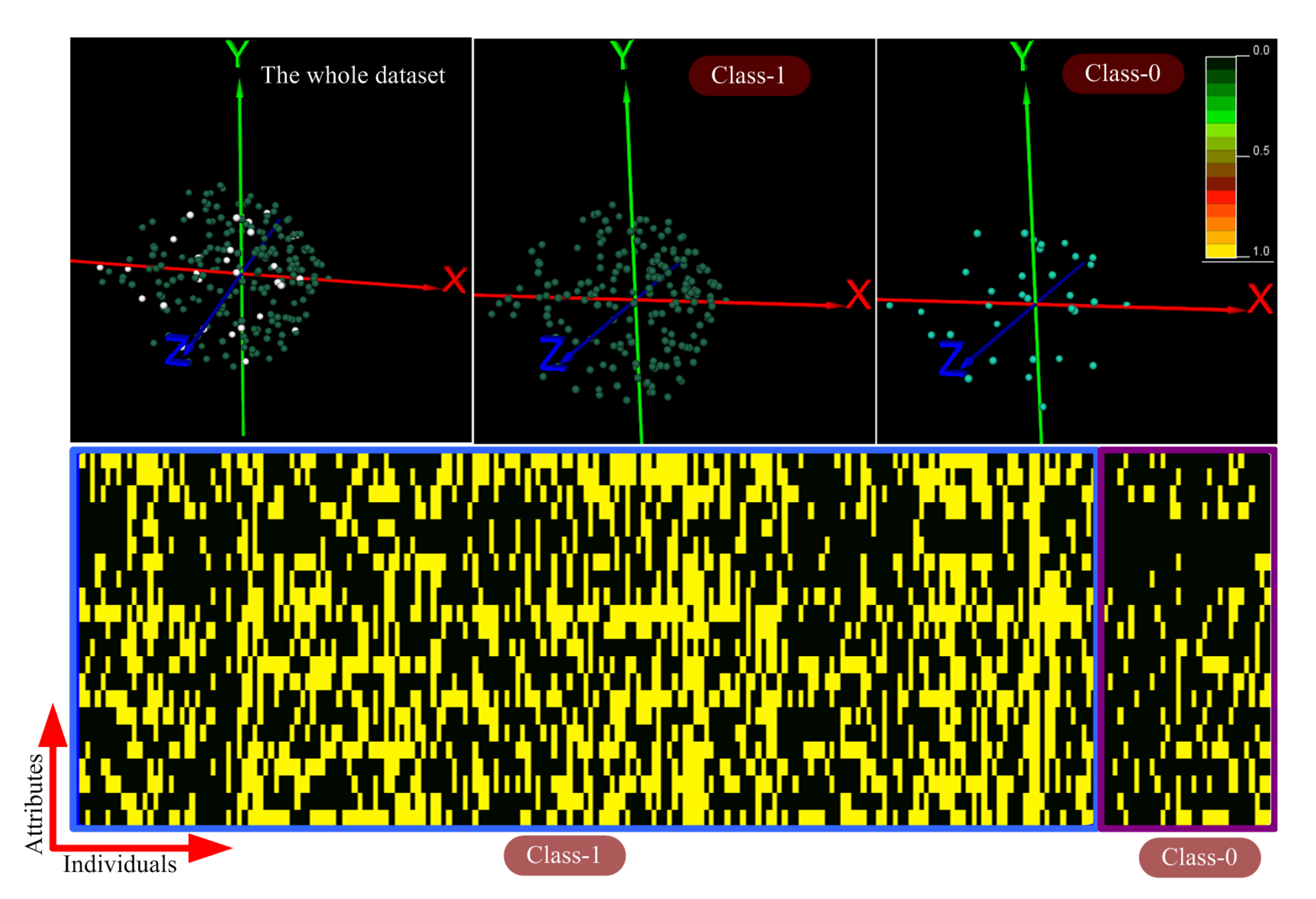
Figure 1. DS1 dataset (Heart Dataset). A 3D-scatterplot is shown at the top of the figure where each point represents a column (an individual) of the dataset showed as a heatmap at the bottom. The dimension of the dataset was reduced to three components by using principal component analysis. In addition, points belonging to each class are shown in different colors. The heatmap corresponding to the same dataset is shown at the bottom of the figure. Each class of the dataset is framed in a box. The color bar shown at the top represents the color scale used in the heatmap.
Processes 08 01565 g001
Figure 2. DS2 dataset (Hepatitis Dataset). A 3D-scatterplot is shown at the top of the figure where each point represents a a column (an individual) of the dataset showed as a heatmap at the bottom. The dimension of the dataset was reduced to three components by using principal component analysis. In addition, points belonging to each class are shown in different colors. The heatmap corresponding to the same dataset is shown at the bottom of the figure. Each class of the dataset is framed in a box. The color bar shown at the top represents the color scale used in the heatmap.
Processes 08 01565 g002
Figure 3. DS3 dataset (Dermatology Dataset). A 3D-scatterplot is shown at the top of the figure where each point represents a column (an individual) of the dataset showed as a heatmap at the bottom. The dimension of the dataset was reduced to three components by using principal component analysis. In addition, points belonging to each class are shown in different colors. The heatmap corresponding to the same dataset is shown at the bottom of the figure. Each class of the dataset is framed in a box. The color bar shown at the top represents the color scale used in the heatmap.
Processes 08 01565 g003
Table 1. Settings given to run the evolutionary method (ESRBC) to build rule-based classifiers for each dataset.
ESRBC SettingsDS1DS2DS3
Population size7050100
Number of generations per rule (fitness function-1)100,000100,000200,000
Number of generations per rule (fitness function-2)200,000200,000400,000
Mutation operator per rule for Algorithm 1 (local search)10,00010,000100,000
Mutation operatorM3M1 and M3M3
Crossover probability0.60.60.6
Mutation probability0.20.30.2
Maximum size of rules (maximum number of clauses)101010
Table 2. Name and description of the methods used in the comparison of the approach proposed.
MethodDescription
SVMLinear Support Vector Machine, which finds the best hyperplane separating both classes.
naiveBayesThis model computes the probability of each class given the values of all attributes and assuming the attribute conditional independence.
KNNk-Nearest Neighbor classification.
This is a lazy model which classifies the input pattern by using its k-Nearest Neighbors from the training set.
ANNArtificial Neural Network implementing a Multilayer Perceptron, which uses a single intermediate layer for our case. Backpropagation and resilient backpropagation have been implemented.
ML-MPCAMaximum Likelihood estimation with Mixture of Principal Component Analyzers.
Bayesian-MPCABayesian approach with Mixture of Principal Component Analyzers.
Table 3. Comparative table of mean accuracy for the evolutionary method (ESRBC) compared with the other machine learning methods.
DatasetMethodAccuracy (%)Youden Index (%)
DS1SVM78.9512.45
naiveBayes46.9314.97
k-NN (k = 3)81.5822.91
ANN79.3912.95
ESRBC81.8240.48
DS2SVM82.5746.91
naiveBayes75.4737.56
k-NN (k = 5)75.4716.47
ANN81.9442.56
ESRBC81.3241.67
DS3ML-MPCA94.9-
Bayesian-MPCA95.8-
ESRBC95.92-
Publisher’s Note: MDPI stays neutral with regard to jurisdictional claims in published maps and institutional affiliations.