Article

A CFD-Based Shape Design Optimization Process of Fixed Flow Passages in a Francis Hydro Turbine

1
Graduate School of Mechanical Engineering, Mokpo National University, Muan 58554, Korea
2
Department of Mechanical Engineering, Institute of New and Renewable Energy Technology Research, Mokpo National University, Muan 58554, Korea
*
Author to whom correspondence should be addressed.
Processes 2020, 8(11), 1392; https://doi.org/10.3390/pr8111392
Submission received: 4 October 2020 / Revised: 27 October 2020 / Accepted: 27 October 2020 / Published: 31 October 2020

Abstract

:
In recent times, optimization began to be popular in the turbomachinery field. The development of computational fluid dynamics (CFD) analysis and optimization technology provides the opportunity to maximize the performance of hydro turbines. The optimization techniques are focused mainly on the rotating components (runner and guide vane) of the hydro turbines. Meanwhile, fixed flow passages (stay vane, casing, and draft tube) are essential parts for the proper flow uniformity in the hydro turbines. The suppression of flow instabilities in the fixed flow passages is an inevitable process to ensure the power plant safety by the reduction of vortex-induced vibration and pressure pulsation in the hydro turbines. In this study, a CFD-based shape design optimization process is proposed with response surface methodology (RSM) to improve the flow uniformity in the fixed flow passages of a Francis hydro turbine model. The internal flow behaviors were compared between the initial and optimal shapes of the stay vane, casing, and the draft tube with J-Groove. The optimal shape design process for the fixed flow passages proved its remarkable effects on the improvement of flow uniformity in the Francis hydro turbine.

1. Introduction

Hydropower is considered a reliable renewable source for electricity production. The hydraulic turbine is an essential component of the hydropower plant. Among various types of hydraulic turbines, Francis turbines are widely used over a wide range of flow rates and heads [1]. The main hydro passage parts of the Francis turbine are composed of a spiral casing, stay vane, guide vane, runner and draft tube. The flow instabilities in the fixed flow passages can cause failure in the whole hydro turbine system. The design of the fixed flow passages is dependent on the moving components of the runner and guide vane in the Francis turbine.
The fixed flow passages are designed to keep the proper flow uniformity by suppressing the pressure pulsation, vortex-induced vibration and swirl flow. The main objective of the stay vane is to maintain the uniform flow from the casing to guide vane and runner flow passages [2]. The non-uniform flow distribution from the stay vane causes the vortex-induced vibration, which initiates the failure in the stay vane [3]. The purpose of the spiral casing is to direct the fluid from the penstock pipe to the stay vane and guide vane. Kurokawa and Nagahara [4] explained the free-vortex, accelerating and decelerating types of the spiral casing. The flow behavior is dependent on the casing shape. The improper flow distribution causes pressure pulsation and secondary vortex, which induces the cracking in the casing wall. Price indicated that the severe pressure fluctuation in the spiral casing causes the brittle crack in the casing wall [5]. The draft tube is designed to improve the dynamic energy in the runner outlet and recover the suction head [6]. The existence of swirl flow in the draft tube causes the flow instabilities [7,8,9]. J-Groove installation suppresses the flow instabilities in the draft tube of the Francis hydro turbine [10]. J-Groove is the groove engraved on the wall of the draft tube that induces reverse jet flow through the shallow groove channels to suppress the swirl flow [11].
The computational fluid dynamics (CFD) analysis has become one of the main tools for turbomachinery flow analysis. The application of CFD analysis makes it easier to evaluate a large number of design cases with precise and accurate results. It is used to predict the internal flow behavior of the turbomachinery, flow separation, and loss distribution in Francis turbine components. Many researchers have conducted CFD analysis on the Francis hydro turbine for the prediction of performance [12], part-load performance [13], suction performance [14], unsteady flow behavior [15]. The CFD analysis and optimization techniques were integrated for the optimization of the runner blade [1]. The maximum improvement in the moving components (runner and guide vane) was achieved via CFD-based optimization [16,17,18,19]. However, few studies related to the fixed flow passages (spiral casing, stay vane and draft tube) of Francis hydro turbines are available [20,21].
Nowadays, design optimization using numerical analysis is widely used for turbomachinery. Wu et al. performed the CFD-based design optimization for a Francis hydro turbine. They showed a comparison between the initial and optimal design of turbines at the design point [19]. They mainly focused on the optimization of the runner blade of the Francis hydro turbine. The conventional blade design approaches integrated with the advanced CFD analysis are powerful and effective tools for the design optimization of turbomachinery. A CFD-based design optimization system that integrates internally developed parametrized mathematical geometry models, automatic mesh generators and commercial 3D Navier–Stokes code like ANSYS CFX 19.2 permits designers to interactively generate, modify and visualize the geometric model of turbine components. The design process can be repeated until a fully optimized model with satisfactory performance is obtained. Nakamura and Kurosawa [22] conducted the design optimization of a high specific speed Francis turbine using a multi-objective genetic algorithm (MOGA). The design optimization of hydraulic machinery can be performed by multilevel CFD techniques [23]. The multilevel CFD technique reduced the computation time. Sosa et al. [6] performed the design optimization of the draft tube by using CFD analysis. Si et al. [24] proposed a multi-point design process based on CFD and an intelligent optimization method for the automotive electronic pump. Ayancik et al. [1] conducted a simulation-based design of a Francis hydro turbine runner that was performed by following a surrogate model-based optimization. The conventional CFD-based design process is executed through trial and error; hence, designing a runner for a Francis hydro turbine can take several months. Due to these drawbacks of conventional CFD-based design, CFD-based optimization design approaches can be followed for the reduction of calculation time and better shape design.
It is essential to integrate a robust and flexible design tool in a CFD-based design optimization system to allow automatic generation and modification of the design geometry. The objective of this study is to propose a CFD-based shape design optimization process for fixed flow passages in the Francis hydro turbine. For the CFD-based shape design optimization, the surrogate model was prepared by using response surface methodology (RSM). The various RSMs were evaluated by the goodness of fit test for the precise and accurate response surface. The multi-objective genetic algorithm (MOGA) was applied for the optimization of the fixed flow passages. The hydraulic design and optimization framework for stay vane, casing, and a draft tube with J-Groove can be generalized for reaction hydro turbines (Francis turbine and Pump turbine). The CFD-based optimization process included the parametric design of stay vane, casing, and the draft tube with J-Groove, fluid domain modeling, meshing, ANSYS CFX solver, post-processing, design of experiment (DOE), response surface preparation and multi-objective optimization.

2. Hydro Turbine Design and Optimization Methodology

2.1. Hydro Turbine Design

2.1.1. Process of Hydraulic Design

Figure 1 illustrates the hydraulic design process of the Francis hydro turbine proposed in this study. The conceptual design of the turbine components is based on the turbomachinery theory. The conceptual design for the Francis hydro turbine was prepared according to the turbine specification. Generally, the hydro turbine design is commenced with the runner design. The guide vane is designed according to the flow angle at the runner inlet. The stay vane design should match the inlet flow angle of the guide vane. The proper flow distribution at the stay vane inlet should be maintained by casing design. The runner outlet flow angle is a constraint for the draft tube design. A fixed flow passage design is linked with each other. Therefore, the initial shape design was completed in serial order as in the conceptual design by theory and detail design by 3D shape modeling. It was challenging to obtain the whole turbine passages optimization at once because it consisted of numerous design variables and overlapping constraints. Hence, the fixed flow passages shape was optimized for each passage separately to reduce the computational cost and make an effective optimization process. In this study, runner and guide vane design conditions were fixed, which created the constraints for the optimization process followed.

2.1.2. Francis Turbine Specification and Performance

The design specification of the 100 MW class Francis hydro turbine model is shown in Table 1. The minimum and maximum heads of the Francis hydro turbine are 66.5 m and 110 m, respectively. The design flow rate of the prototype turbine is 125.4 m3/s. The turbine maximum output power is 113 MW, and the minimum output power is 62.3 MW. The specific speed Ns, unit discharge Q11 and unit speed N11 are evaluated by using Equations (1)–(3), respectively.
N s = n P H 5 4
Q 11 = Q D e 2 H
N 11 = n D e H
where n is the rotational speed in min−1, P is the output power in kW, H is effective head in m, Q is flow rate in m3/s, De is the runner outlet diameter.
Francis turbine fluid domain by initial design is shown in Figure 2a, which consists of a spiral casing, 20 stay vanes, and 20 guide vanes with 13 runner blades, and the elbow-type draft tube. The runner inlet and outlet diameters are Di = 4863 mm and De = 3995 mm, respectively. The installed capacity of the Francis turbine is 100 MW. The efficiency hill chart of the Francis hydro turbine by initial design and CFD analysis is shown in Figure 2b. The various guide vane openings are used to regulate the flow rate for the Francis hydro turbine. The guide vane opening from 8° to 41° is used to change the flow rate. The design point for the Francis hydro turbine is determined at N11 = 76.12 and Q11 = 0.87. The best efficiency of the Francis hydro turbine is located in the range of guide vane angles of 23° to 26° and unit speeds of N11 = 70 to N11 = 80.

2.1.3. Stay Vane Design

The purpose of the stay vane (SV) is to guide the water flow from the casing to guide vane and runner, and for structural purpose. The main design parameters for the stay vane are vane angles, thickness, ellipse ratio at the leading edge, and trailing edge. The design parameters for the stay vane are shown in Figure 3a. The design parameters for the stay vane are defined as in Equation (4).
d S V = [ α 1 ,   , α 5 , δ 1 , , δ 5 , a l e , a t e ] T
where d S V is the design variables matrix of the stay vane, αi is the vane angle at ith section of the stay vane, δi is the thickness at ith section of the stay vane, ale is the ellipse ratio at the leading edge (LE), ate is the ellipse ratio at the trailing edge (TE) and superscript T indicates the transpose of the design variables matrix.
Figure 3b shows the initial stay vane shape using the vane angle and thickness distributions. The inlet vane angle is 30°, and the outlet vane angle is 33°. The thickness of the stay vane is 46 mm at the LE and 28 mm at the TE. The maximum thickness of the stay vane is 150 mm at 0.4 normalized distance from the LE. The vane angle and thickness distribution are the same throughout the stay vane.

2.1.4. Casing Design

The spiral casing shape is dependent on the cross-section radii [20]. Figure 4a,b indicates the parametric design parameters and initial shape design of the casing, respectively. The parametric design of the casing shape is defined as in Equation (5).
d C A = [ r 0 , r 2 , , r 11 ] T
where d C A is the design variables matrix of the casing, ri is the cross-section radius at ith section of the spiral casing.

2.1.5. Draft Tube Design with J-Groove Installation

The diffuser angle of the draft tube is generally determined in the range of 3° to 10° for minimum energy loss, which is an important design parameter for the discharge pressure recovery and flow uniformity in the draft tube [25]. The conceptual design of the draft tube shows that the diffuser angle of 3.5° provides maximum pressure recovery. Figure 5 shows the technical design of the draft tube. Moreover, in the case of the off-design condition, there exists swirl flow in the draft tube of the Francis hydro turbine, and J-Grooves can be an effective countermeasure of the flow instability in the draft tube [10]. J-Grooves are the grooves that are installed on the draft tube inner wall of the Francis turbine. The design parameters of the J-Groove are defined as angle (θJG), length (lJG), depth (dJG) and number (nJG), which are shown in Figure 6. The J-Groove is used to suppress the swirl flow in the draft tube by the reverse flow mechanism through the J-Groove passage [11].
The parametric design for the J-Groove is represented in Equation (6).
d D T = [ d J G , θ J G , l J G , n J G ] T ,
where d D T is the design variable matrix of the J-Groove, dJG is the J-Groove depth, θJG is the J-Groove angle, lJG is the J-Groove length and n J G is the number of J-Grooves.
The grooves are evenly distributed in the circumference of the draft tube. Therefore, the number of J-Grooves can be calculated as in Equation (7). The initial shape of the J-Groove is defined as dJG = 106 mm, lJG = 2000 mm, θJG = 12° and n J G = 15.
n J G = 180 ° θ J G

2.2. Optimization Methodology

2.2.1. Process of Shape Optimization

The optimization process for the shape optimization of Francis hydro turbine fixed flow passages is illustrated in Figure 7. The design of experiments (DOE) was generated by using the optimal-space filling (OSF) method. The optimization for the fixed flow passages was carried out by using response surface methodology (RSM) and multi-objective genetic algorithm (MOGA). RSM is considered a sensitivity analysis tool, which is used to improve the sensitivity between the objective functions and input parameters [26]. RSM can be expressed as in Equation (8). The RSM uses a first-order and second-order polynomial form to develop the precise and concise correlation model, and the mathematical expressions of RSM are shown in Equations (9) and (10):
y = f ( x 1 , x 2 , , x n ) + e
y = α ο + i = 1 n α i x i + e 1
y = α ο + i = 1 n α i x i + i = 1 n α i i x i 2 + i = 1 n 1 j = i + 1 n α i j x i x j + e 2
where y is the response of the system, x1, x2, ⋯, xn are the independent variables and e is the error, xi is the ith input parameter, α is the coefficient of the response surface.
RSM was used to decrease the computational cost in the optimization process. The response surface for the objective functions can be generated by using various RSMs such as genetic aggregation (GA) [27], radial basis function (RBF) [28], polynomial response surface (PRS) [29], Kriging (KG) [30], non-parametric regression (NPR) [31], neural network (NN) [32]. All these methodologies have their pros and cons. The selection of the RSM is based on the accuracy and consistency of the methodology. Among different RSMs, the accuracy is measured by using the goodness of fit test. The goodness of fit test can be calculated by using the coefficient of determination (CoD), maximum relative residual (MRR) and root mean square error (RMSE), which are expressed in Equations (11)–(13).
C o D = 1 i = 1 n s ( y i y ^ i ) 2 i = 1 n s ( y i y ¯ i ) 2
M R R = max i [ A b s ( y i y ^ i y ¯ ) ]
R M S E = 1 n s i = 1 n s ( y i y ^ i ) 2
where ns is the number of verification points, yi is the response from CFD analyses, y ^ i is the corresponding response from the surrogate model and y ¯ is the arithmetic mean of yi. The verification points are used to evaluate Equations (11)–(13). If the result of the goodness measure shows CoD = 100%, MRR = 0% and RSME = 0%, it means that the response surface is highly precise and accurate.
The goodness measures concluded that the genetic aggregation was most suitable for the approximation of response surface, compared to other RSMs. The results of the goodness of fit test are shown in Table 2. Therefore, in this study, the genetic aggregation method was implied for the preparation of the response surface. The optimization was carried out using MOGA. Table 3 indicates the setting criteria for the optimization process.

2.2.2. Process of Stay Vane Shape Optimization

In this study, the turbine efficiency η ( d S V ) , flow uniformity γ ( d S V ) , head loss H l ( d S V ) , effective head H ( d S V ) , and flow rate Q ( d S V ) were considered for the evaluation of stay vane design as in Equations (14)–(18). The measurement locations of the flow uniformity at SVout and head loss are calculated by the difference between the total pressure at SVin and SVout, as shown in Figure 3.
η ( d S V ) = [ τ ω ρ g Q H ] × 100 %
γ ( d S V ) = [ 1 ( u ¯ u ) 2 2 A u ¯ d A ] × 100 %
H l ( d S V ) = Δ p t o t a l @ S V ρ g
H ( d S V ) = p t i n l e t p t o u t l e t ρ g
Q ( d S V ) = m o u t l e t ρ
where τ is torque generated by runner (Nm) and ω is rotational speed of runner (rad/s). u ¯ is the average velocity in stay vane passage (m/s), u is the local velocity in stay vane passage (m/s) and A is the cross-section area of stay vane passage (m2). Δ p t o t a l @ S V is the change in total pressure in stay vane passage (Pa), p t i n l e t and p t o u t l e t are total pressures at inlet and outlet of the turbine (Pa). m o u t l e t is mass flow rate of water at the turbine outlet (kg/s).
The optimization formulation for the stay vane is elaborated as in Equation (19).
maximize   η ( d S V ) ,   γ ( d S V ) minimize   H l ( d S V ) subject   to   80   m H ( d S V ) 95   m 120   m 3 / s Q ( d S V ) 135   m 3 / s d S V L d S V d S V U
where d S V L and d S V U are lower and upper bounds for the design variable d S V , respectively, and their values are summarized in Table 4. The turbine efficiency η ( d S V ) and flow uniformity γ ( d S V ) were maximized to obtain more output power, while vortex-induced vibration was suppressed. At the same time, the head loss H l ( d S V ) was minimized to prevent loss of power in the stay vane. The effective head H ( d S V ) and flow rate Q ( d S V ) of the turbine were used as constraints for the stay vane design.
The optimal Pareto front for the stay vane design is shown in Figure 8. The Pareto front is plotted between turbine efficiency and flow uniformity. The trade-off between turbine efficiency and flow uniformity is required to obtain the optimal design of stay vane. Flow uniformity is measured at the outlet of the stay vane. The measuring location plays a vital role in the calculation of flow uniformity. If the measuring location changes, the nature of the Pareto front will change. The main objective of the design optimization is to have smooth flow distribution in the stay vane flow passage. The flow uniformity of the optimal stay vane should be above 90%. Based on the above assumptions, the optimal stay vane (OSV) was selected with flow uniformity 91.97% and turbine efficiency 96.37%.

2.2.3. Process of Casing Shape Optimization

In order to evaluate the flow condition in the casing, the flow uniformity γ ( d C A ) and head loss H l ( d C A ) were examined. The flow uniformity, which determines the deviation of flow velocity in the casing shape, is calculated as in Equation (20). The flow uniformity was measured as an averaged value at the location of the whole casing outlet of 1.00 De from the runner axis center, which is shown in Figure 4a by a red circle. The head loss was defined by the losses in the spiral casing passage due to flow mixing and wall friction, as in Equation (21), and the head loss was calculated by the difference between inlet and outlet of casing.
γ ( d C A ) = [ 1 ( u ¯ u ) 2 2 A u ¯ d A ] × 100 %
H l ( d C A ) = Δ p t o t a l @ c a s i n g ρ g
where u ¯ is the average velocity in casing passage (m/s), u is the local velocity in casing passage (m/s), and A is the cross-section area of casing passage (m2), Δ p t o t a l @ c a s i n g is change in total pressure in casing passage (Pa).
The design optimization problem of the casing is formulated as in Equation (22).
maximize   γ ( d C A ) minimize   H l ( d C A ) subject   to   γ ( d C A ) 97 % d C A L d C A d C A U
where d C A L and d C A U are lower and upper bounds for the design variable d C A , respectively.
The bounds for design variables of the casing are shown in Table 5. The Pareto front for the casing shape optimization was prepared by using head loss and flow uniformity. Figure 9 shows the Pareto front for the optimization of the casing. The Pareto front shows the trade-off between flow uniformity and head loss. Thus, the selection of the optimal design is based on the requirement of the user. In this study, the main objective was to increase the flow uniformity above 97%. Therefore, the optimal design was selected considering flow uniformity above 97% with minimum head loss.

2.2.4. Process of Draft Tube Shape Optimization

The optimization was carried out to obtain the optimal solution for the draft tube shape with the J-Groove installation. The turbine efficiency η ( d D T ) , swirl intensity S ( d D T ) , head loss H l ( d D T ) , effective head H ( d D T ) , and flow rate Q ( d D T ) were considered for the evaluation of draft tube shape design, as in Equations (23)–(25). The measurement locations of the swirl intensity were set in the range of z/R0 = 1.15 to 3.60, as shown in Figure 6.
η ( d D T ) = [ τ ω ρ g Q H ] × 100 %
S ( d D T ) = v θ v a r 2 d r R v a 2 r d r
H l ( d D T ) = Δ p t o t a l @ J G ρ g
where τ is torque generated by runner (Nm), ω is rotational speed of runner (rad/s), ρ =997 kg/m3 is the density of water at 25 ℃, g = 9.81 m/s2 is gravitational acceleration, Q is the flow rate (m3/s), and H is the effective head (m), v θ is the local tangential velocity in the draft tube (m/s), v a is the local axial velocity in the draft tube, r is the radial position, R is the cross-section radius, Δ p t o t a l @ J G is the change in total pressure in draft tube passage (Pa), z is the vertical distance from the axis of turbine, R0 is the runner outlet radius.
In order to investigate the flow instability and to express the complicated and unique internal flow behavior in the draft tube effectively, swirl intensity S ( d D T ) was adopted to determine the strength of swirl flow in the draft tube. The swirl intensity represents the ratio of the axial flux of angular momentum to axial momentum, as shown in Equation (24).
The optimization formulation for the draft tube is elaborated as in Equation (26).
maximize   η ( d D T ) minimize   S ( d D T ) ,   H l ( d D T ) subject   to   80   m H ( d D T ) 95   m 120   m 3 / s Q ( d D T ) 135   m 3 / s d D T L d D T d D T U ,
where d D T L and d D T U are lower and upper bounds for the design variable d D T , respectively, and their values are summarized in Table 6. The turbine efficiency η ( d D T ) was maximized to obtain more output power. At the same time, the swirl intensity S ( d D T ) and head loss H l ( d D T ) were minimized to suppress the swirl flow and prevent energy loss in the draft tube flow passage. The effective head H ( d D T ) and flow rate Q ( d D T ) of the turbine were used as constraints for the draft tube design, which are expressed as in Equations (17) and (18), respectively.
The lower and upper limits of draft tube design variables are indicated in Table 6.
The optimization of the draft tube design was carried out at the design point. The Pareto front was prepared by the trade-off between turbine efficiency and swirl intensity, which is shown in Figure 10.

3. CFD Methodology

The CFD analysis for the turbomachinery requires a highly reliable computational system for the calculation of complex internal flow phenomena. Moreover, while conducting the optimization, numerous samples are needed, which demand extensive computational cost and time for CFD analysis. Figure 11 shows the numerical scheme of CFD analysis adopted in this study, in combination with the optimal design process. The CFD analysis process is directly connected to the optimum design process. The CFD analysis method was adopted from previous studies [33,34,35].
The CFD analysis for the casing DOE samples was performed without stay vanes because the flow field in the spiral casing is independent of the flow field of the stay vane [36]. Furthermore, the single flow passage analysis for the stay vane was used for the calculation of DOE. It provides precise CFD analysis results and reduces the computation time. However, the full domain analysis was required for the DOE of the draft tube with the J-Groove installation because the flow field in the J-Groove is dependent on other components of the Francis hydro turbine.
The CFD analysis was conducted using a commercial code of ANSYS CFX 19.2 [37]. The numerical analysis was performed by solving the governing equations and Reynolds-averaged Navier–Stokes (RANS) with the turbulence model. In this study, the Shear Stress Transport (SST) turbulence model was selected because the SST model combines the capabilities of the κ-ω model away from the walls and the robustness of the κ-ε turbulence near the walls by using blending functions of the automatic near-wall treatment. The Rhie–Chow algorithm was used to interpolate the pressure–velocity coupling mechanism. The high-resolution order was used to solve the advection term, and the first-order upwind difference was used to solve the turbulence numeric [37].
The proper numerical grids are required for precise and accurate computational analysis. The structured mesh for the numerical analysis was generated using ANSYS ICEM 19.2 [37]. The numerical grids for the 100 MW class Francis hydro turbine are shown in Figure 12. The mesh dependence test was carried out to determine the optimum number of nodes. The results of the mesh dependence were compared with efficiency and output power. Figure 13 shows the mesh dependence test results, and we concluded that 8.2 million nodes was the optimum number for computational analysis. Table 7 presents the information on the numerical grids used for CFD analysis. The non-dimensional wall distance y+ values for the several components of the Francis hydro turbine were less than 100, which was suitable for the SST turbulence model with automatic near-wall treatment within the reliable resolution range of 1 < y + < 100. Table 8 shows the summary of boundary conditions for CFD analysis. The performance curves of the 100 MW Francis hydro turbine are shown in Figure 14. The performance curves indicated that the design point and best efficiency point were matched well. They verified that the conceptual design of the 100 MW Francis hydro turbine was acceptable.

4. Results and Discussion

4.1. Stay Vane Shape Optimization

Figure 15 shows the comparison of the vane angle and thickness between the initial stay vane (ISV) and optimal stay vane (OSV) shapes. The inlet vane angle was changed from 30° to 32°. The position for the maximum thickness was modified from the normalized distance of 0.4 to 0.3. The maximum thickness was increased from 150 mm to 158 mm. The 3D view of the initial and optimal stay vane shapes are shown in Figure 15. Table 9 shows the results of stay vane optimization for the 100 MW class Francis turbine. The targeted objectives of turbine efficiency, flow uniformity and head loss were all improved remarkably.
The flow uniformity was measured at the outlet of the stay vane. The flow uniformity encountered the average deviation of local velocity in the reference area. The flow deviation in the small section did not show a significant effect on flow uniformity. Therefore, flow angle distribution and vorticity were evaluated for internal flow patterns in stay vane passage. The comparison of the flow angle between the ISV and OSV is shown in Figure 16. The flow angle (θu) is defined by Equation (27).
θ u = tan 1 ( v θ v r )
where vθ and vr are tangential and radial velocity components.
Figure 16 shows the comparison of flow angle in the ISV and OSV at the design point. The peak value of the flow angle at the hub and shroud indicated the occurrence of the secondary flow near the hub and shroud walls. The flow angle difference in the passage between the outlet of stay vane and inlet of guide vane in the OSV became remarkably smaller than that of the ISV. It meant that the OSV had a relatively larger ability to maintain a proper flow angle. The smaller difference caused the lower vorticity in the passage between the stay vane and guide vane in the OSV.
Figure 17 shows the strength of vorticity in between the cascade passages of the stay vane and guide vane. The decrease in the vorticity at the OSV flow passage made the flow smoother. Thus, the possibility of occurrence of secondary flow and vortices at the OSV flow passage decreased significantly in the OSV. Therefore, the OSV made a more uniform flow distribution in the vane’s passage.

4.2. Casing Shape Optimization

Figure 18 indicates the cross-section radius comparison between the initial and optimal shape of the casing. The cross-section radius of the optimal casing shape was greater than the initial casing shape at the central angles below θ = 180°, but the cross-section radius near the casing tongue of θ = 345° was almost the same.
Table 10 shows the flow uniformity and head loss by the initial and optimal casing shapes, which was compared to the design point. The flow uniformity increased slightly in the optimal casing in comparison with that of the initial casing shape; furthermore, the optimal casing design showed a significant decrease in the head loss in comparison with that of the initial casing design.
The secondary vortex intensity J A B S n was used to evaluate the internal flow behavior in the casing quantitatively. The area integral of vorticity around the casing was calculated as defined in Equation (28).
J A B S n = 1 A 0 A | × u n | d A
where u n is the velocity at normal direction to the cross section, A is the cross section area.
Figure 19 shows the comparison of secondary vortex intensity between the initial and optimal casing designs. The secondary vortex intensity is in increasing order from the inlet to the casing tongue. The vortex intensity was suppressed significantly by optimal design in comparison to the initial casing shape. Therefore, it was clear that the flow uniformity and head loss could be improved effectively by the current optimum design process.

4.3. Draft Tube Shape Optimization

Table 11 shows the comparison of the design parameter sizes of the J-Grooves for draft tube shape optimization. The 3D model of the J-Grooves installed on the draft tube wall is shown in Figure 20.
Figure 21 shows the comparison of the swirl intensity in the draft tube by J-Groove shapes at the design point. The swirl intensity was suppressed significantly with the installation of J-Groove. There was a 12.12% swirl intensity reduction with initial J-Groove installation from the case without J-Groove installation. Moreover, the additional 6.64% swirl intensity reduction was achieved by the optimized J-Groove shape from the initial J-Groove shape. Therefore, it was clear that the installation of an optimal J-Groove in the draft tube had a significant effect on the suppression of the flow instability caused by the swirl flow. Table 12 reveals the results summary of the draft tube shape optimization. The study results indicated that the installation of the J-Groove on the wall of the draft tube had almost no influence on the turbine performance but suppressed the flow instability of the swirl flow remarkably.

5. Conclusions

In the present study, the fixed flow passage shapes of a 100 MW class Francis hydro turbine were optimized for the internal flow uniformity by a CFD-based shape design optimization process. The stay vane, casing, and draft tube were optimized separately to understand the flow characteristics in each flow passage. The objective of the optimization was to maximize the flow uniformity and minimize the head loss in each flow passage.
A CFD-based shape design optimization process of the parametric conceptual design, detailed design, and optimal design of the fixed flow passage of the Francis hydro turbine was accomplished. The design and optimization process can be generalized for the reaction hydro turbine stay vane, casing, and draft tube with J-Grooves. Moreover, better flow uniformity was achieved in the Francis hydro turbine by the fixed flow passages optimization process. For the optimization process, response surface methodology was used to generate the response surface, and a multi-objective genetic aggregation method was used to determine the global optimum solution via the optimal Pareto front.
The optimum stay vane shape was achieved with the remarkably decreased vorticity around the stay vane flow passage, which resulted in the highly improved flow uniformity in the vane passage. The optimal casing passage shape was achieved with the increased flow uniformity and the significantly decreased head loss in comparison with that of the initial casing shape. The secondary vortex intensity was suppressed effectively by casing shape optimization. The installation of a J-Groove on the wall of the draft tube had almost no influence on the turbine performance but suppressed the flow instability of swirl flow remarkably in the draft tube passage.

Author Contributions

Conceptualization, U.S., and Y.-D.C.; methodology, U.S.; software, Y.-D.C.; validation, U.S. and Y.-D.C.; formal analysis, U.S.; investigation, U.S.; resources, Y.-D.C.; data curation, U.S.; writing—original draft preparation, U.S.; writing—review and editing, U.S. and Y.-D.C.; visualization, U.S.; supervision, Y.-D.C.; project administration, Y.-D.C.; funding acquisition, Y.-D.C. All authors have read and agreed to the published version of the manuscript.
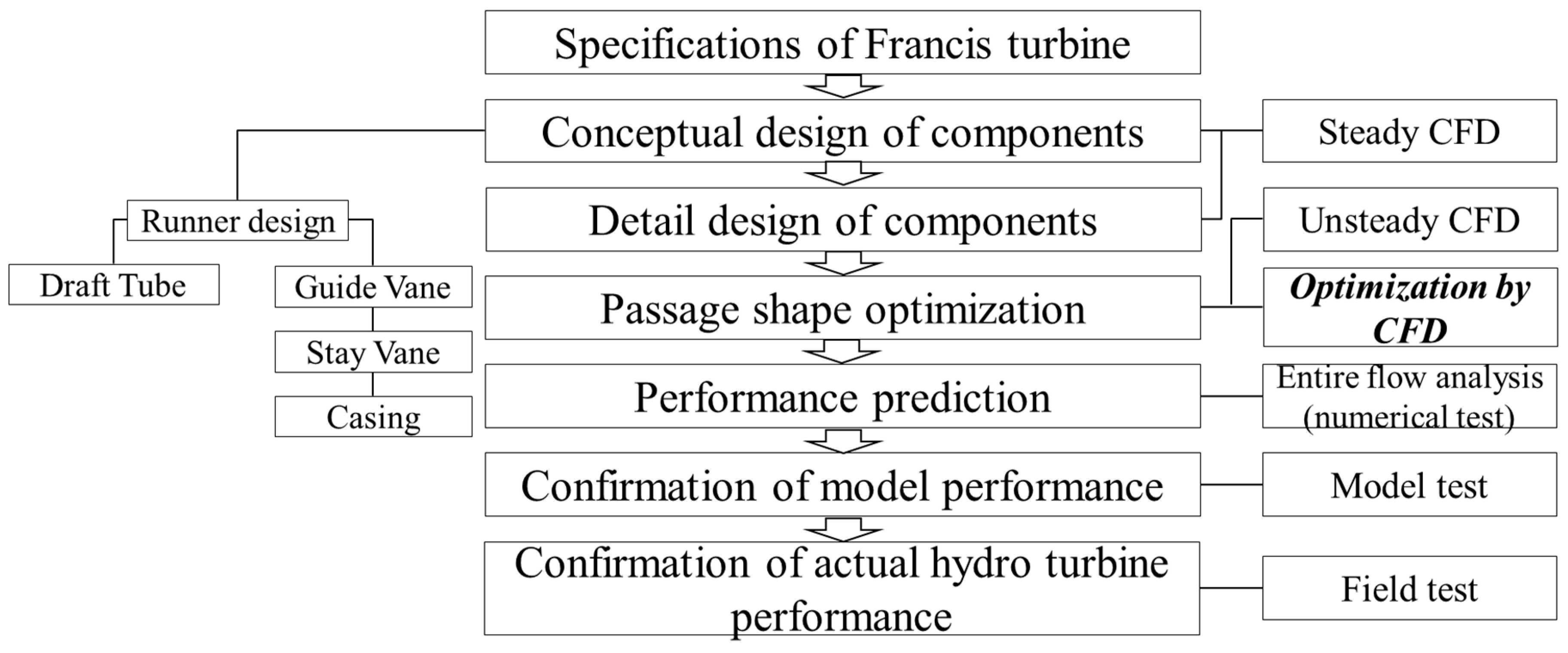
Funding

This work was supported by the New and Renewable Energy of the Korea Institute of Energy Technology Evaluation and Planning (KETEP), which was funded by the Korean Government Ministry of Trade, Industry and Energy (no. 20163010060350).

Conflicts of Interest

The authors declare no conflict of interest.

References

  1. Ayancik, F.; Acar, E.; Çelebioğlu, K.; Aradag, S. Simulation-based design and optimization of Francis turbine runners by using multiple types of metamodels. Proc. Inst. Mech. Eng. Part C J. Mech. Eng. Sci. 2016, 231, 1427–1444. [Google Scholar] [CrossRef]
  2. Goldwag, E.; Berry, D.G. Von Karman Hydraulic Vortexes Cause Stay Vane Cracking on Propeller Turbines at the Little Long Generating Station of Ontario Hydro. J. Eng. Power 1968, 90, 213–217. [Google Scholar] [CrossRef]
  3. Fischer, R.; Gummer, J.; Liess, C. Stay vane vibrations in the Nkula Falls turbines. Hydropower Dams 1994, 1, 15–20. [Google Scholar]
  4. Kurokawa, J.; Nagahara, H. Flow characteristics in spiral casing of water turbines. In Proceedings of the 13th International Association for Hydraulic Research Symposium on Hydraulic Machinery and Cavitation, Montreal, QC, Canada, 2–5 September 1986. [Google Scholar]
  5. Price, J.W.H. The failure of the Dartmouth turbine casing. Int. J. Press. Vessel. Pip. 1998, 75, 559–566. [Google Scholar] [CrossRef]
  6. Sosa, J.B.; Urquiza, G.; García, J.C.; Castro, L.L. Computational fluid dynamics simulation and geometric design of hydraulic turbine draft tube. Adv. Mech. Eng. 2015, 7, 1–11. [Google Scholar] [CrossRef] [Green Version]
  7. Favrel, A.; Müller, A.; Landry, C.; Yamamoto, K.; Avellan, F. Study of the vortex-induced pressure excitation source in a Francis turbine draft tube by particle image velocimetry. Exp. Fluids 2015, 56, 1–15. [Google Scholar] [CrossRef]
  8. Susan-Resiga, R.; Ciocan, G.D.; Anton, I.; Avellan, F. Analysis of the Swirling Flow Downstream a Francis Turbine Runner. J. Fluids Eng. 2006, 128, 177–189. [Google Scholar] [CrossRef]
  9. Susan-Resiga, R.; Muntean, S.; Avellan, F.; Anton, I. Mathematical modelling of swirling flow in hydraulic turbines for the full operating range. Appl. Math. Model. 2011, 35, 4759–4773. [Google Scholar] [CrossRef]
  10. Chen, Z.; Singh, P.M.; Choi, Y.-D. Suppression of unsteady swirl flow in the draft tube of a Francis hydro turbine model using J-Groove. J. Mech. Sci. Technol. 2017, 31, 5813–5820. [Google Scholar] [CrossRef]
  11. Choi, Y.-D.; Shrestha, U. Cavitation Performance Improvement of an Annular Jet Pump by J-Groove. KSFM J. Fluid Mach. 2020, 23, 25–35. [Google Scholar] [CrossRef]
  12. Oh, H.W.; Yoon, E.S. Application of computational fluid dynamics to performance analysis of a Francis hydraulic turbine. Proc. Inst. Mech. Eng. Part A J. Power Energy 2007, 221, 583–590. [Google Scholar] [CrossRef]
  13. Goyal, R.; Trivedi, C.; Gandhi, B.K.; Cervantes, M.J. Numerical simulation and validation of a high head model francis turbine at prat load operating condition. J. Inst. Eng. India Series C 2018, 99, 557–570. [Google Scholar] [CrossRef]
  14. Escaler, X.; Roig, R.; Hidalgo, V. Sensitivity Analysis of Zwart-Gerber-Belamri Model Parameters on the Numerical Simulation of Francis Runner Cavitation. In Proceedings of the 10th International Symposium on Cavitation (CAV2018), Baltimore, MD, USA, 14–16 May 2018; pp. 911–914. [Google Scholar]
  15. Agnalt, E.; Iliev, I.; Solemslie, B.W.; Dahlhaug, O.G. On the Rotor Stator Interaction Effects of Low Specific Speed Francis Turbines. Int. J. Rotating Mach. 2019, 2019, 1–11. [Google Scholar] [CrossRef]
  16. Leguizamón, S.; Avellan, F. Open-Source Implementation and Validation of a 3D Inverse Design Method for Francis Turbine Runners. Energies 2020, 13, 2020. [Google Scholar] [CrossRef] [Green Version]
  17. Kaewnai, S.; Wongwises, S. Improvement of the Runner Design of Francis Turbine using Computational Fluid Dynamics. Am. J. Eng. Appl. Sci. 2011, 4, 540–547. [Google Scholar] [CrossRef]
  18. Obrovsky, J.; Krausova, H.; Spidla, J.; Zouhar, J. Development of high specific speed Francis turbine for low head HPP. Eng. Mech. 2013, 20, 139–148. [Google Scholar]
  19. Wu, J.; Shimmei, K.; Tani, K.; Niikura, K.; Sato, J. CFD-Based Design Optimization for Hydro Turbines. J. Fluids Eng. 2007, 129, 159–168. [Google Scholar] [CrossRef]
  20. Shrestha, U.; Choi, Y.-D. Improvement of flow behavior in the spiral casing of Francis hydro turbine model by shape optimization. J. Mech. Sci. Technol. 2020, 34, 1–10. [Google Scholar] [CrossRef]
  21. McNabb, J.; Devals, C.; Kyriacou, S.A.; Murry, N.; Mullins, B.F. CFD based draft tube hydraulic design optimization. IOP Conf. Series Earth Environ. Sci. 2014, 22, 12023. [Google Scholar] [CrossRef] [Green Version]
  22. Nakamura, K.; Kurosawa, S. Design Optimization of a High Specific Speed Francis Turbine Using Multi-Objective Genetic Algorithm. Int. J. Fluid Mach. Syst. 2009, 2, 102–109. [Google Scholar] [CrossRef]
  23. Thum, S.; Schilling, R. Optimization of Hydraulic Machinery Bladings by Multilevel CFD Techniques. Int. J. Rotating Mach. 2005, 2005, 161–167. [Google Scholar] [CrossRef] [Green Version]
  24. Si, Q.; Lu, R.; Shen, C.; Xia, S.; Sheng, G.; Yuan, J. An Intelligent CFD-Based Optimization System for Fluid Machinery: Automotive Electronic Pump Case Application. Appl. Sci. 2020, 10, 366. [Google Scholar] [CrossRef] [Green Version]
  25. Balje, O.E.; Japikse, D. Turbomachines—A Guide to Design Selection and Theory; John Wiley & Sons: Hoboken, NJ, USA, 1981; p. 163. [Google Scholar]
  26. Bauer, K., Jr.; Parnell, G.S.; Meyers, D.A. Response surf Formatting. ace methodology as a sensitivity analysis tool in decision analysis. J. Multi Criteria Decision Anal. 1999, 8, 162–180. [Google Scholar] [CrossRef]
  27. Wang, S.; Jian, G.; Xiao, J.; Wen, J.; Zhang, Z. Optimization investigation on configuration parameters of spiral-wound heat exchanger using Genetic Aggregation response surface and Multi-Objective Genetic Algorithm. Appl. Therm. Eng. 2017, 119, 603–609. [Google Scholar] [CrossRef]
  28. Amouzgar, K.; Strömberg, N. Radial basis functions as surrogate models with a priori bias in comparison with a posteriori bias. Struct. Multidiscip. Optim. 2016, 55, 1453–1469. [Google Scholar] [CrossRef] [Green Version]
  29. Acar, E.; Raisrohani, M. Ensemble of metamodels with optimized weight factors. Struct. Multidiscip. Optim. 2008, 37, 279–294. [Google Scholar] [CrossRef]
  30. Liu, H.; Maghsoodloo, S. Simulation optimization based on Taylor Kriging and evolutionary algorithm. Appl. Soft Comput. 2011, 11, 3451–3462. [Google Scholar] [CrossRef]
  31. Wang, Q. Nonparametric regression function estimation with surrogate data and validation sampling. J. Multivar. Anal. 2006, 97, 1142–1161. [Google Scholar] [CrossRef] [Green Version]
  32. Melo, A.P.; Cóstola, D.; Lamberts, R.; Hensen, J.L.M. Development of surrogate models using artificial neural network for building shell energy labelling. Energy Policy 2014, 69, 457–466. [Google Scholar] [CrossRef] [Green Version]
  33. Chen, Z.; Singh, P.M.; Choi, Y.-D. Francis Turbine Blade Design on the Basis of Port Area and Loss Analysis. Energies 2016, 9, 164. [Google Scholar] [CrossRef] [Green Version]
  34. Chen, Z.; Choi, Y.-D. Suppression of cavitation in the draft tube of Francis turbine model by J-Groove. Proc. Inst. Mech. Eng. Part C J. Mech. Sci. 2018, 233, 3100–3110. [Google Scholar] [CrossRef]
  35. Singh, P.M.; Chen, Z.; Choi, Y.-D. Hydraulic design and performance analysis on a small pump-turbine system for ocean renewable energy storage system. J. Mech. Sci. Technol. 2017, 31, 5089–5097. [Google Scholar] [CrossRef]
  36. Maji, P.K.; Biswas, G. Three-dimensional analysis of flow in the spiral casing of a reaction turbine using a differently weighted Petrov Galerkin method. Comput. Methods Appl. Mech. Eng. 1998, 167, 167–190. [Google Scholar] [CrossRef]
  37. ANSYS. ANSYS CFX Documentation; ANSYS Inc.: Canonsburg, PA, USA, 2017. [Google Scholar]
Figure 1. Hydraulic design process of the Francis hydro turbine with computational fluid dynamics (CFD)-based optimization.
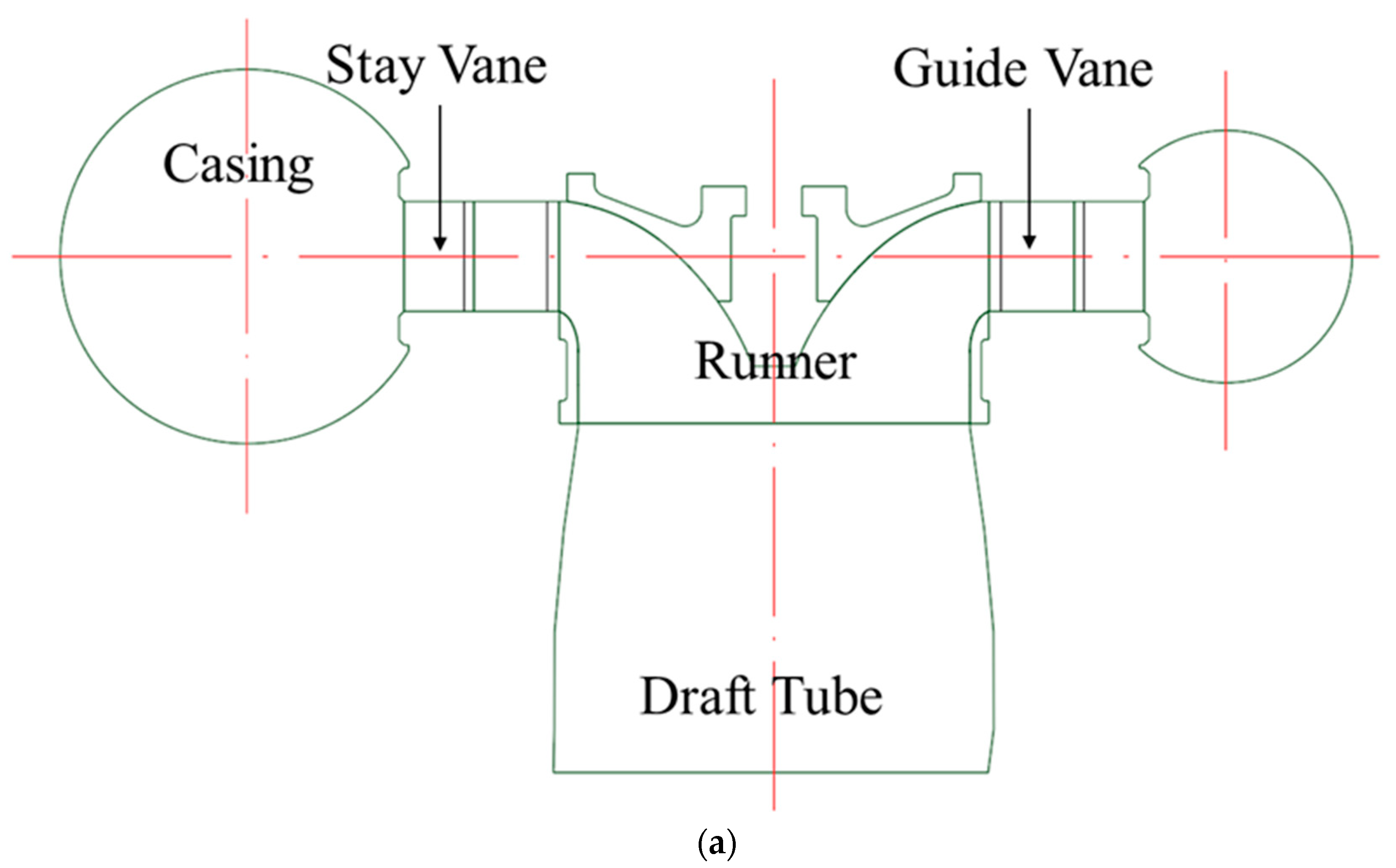
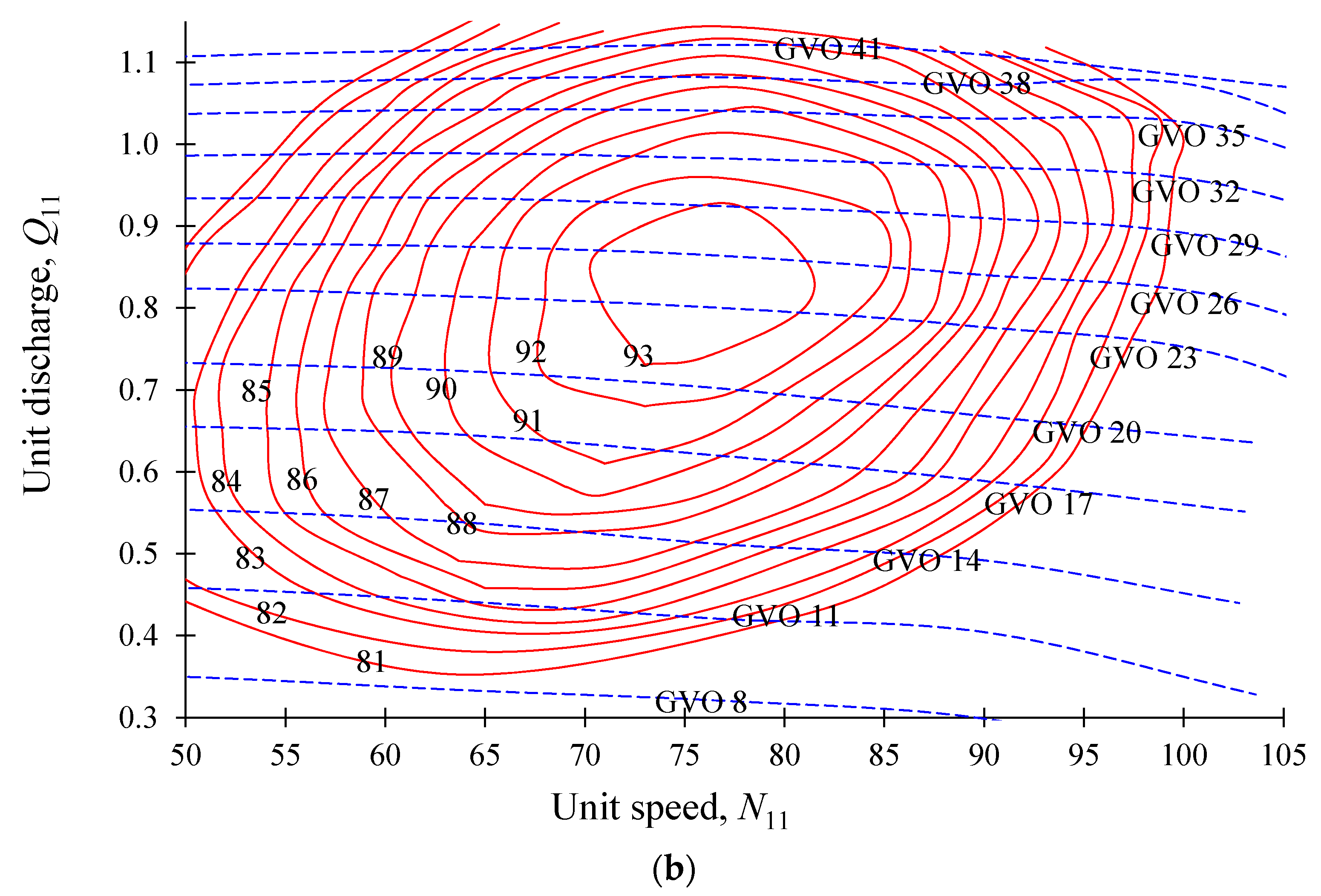
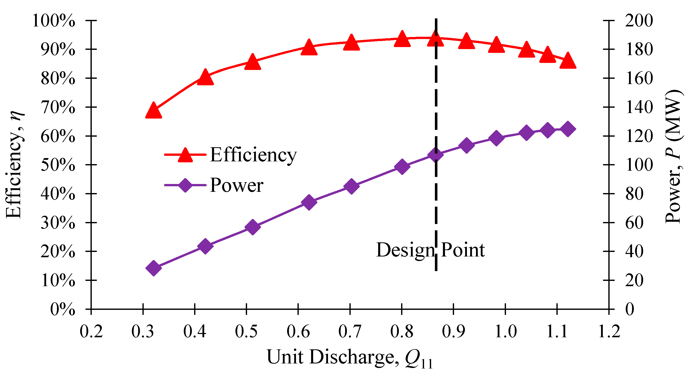
Processes 08 01392 g001
Figure 2. (a) Schematic view and (b) efficiency hill chart of the 100 MW class Francis hydro turbine by initial design.
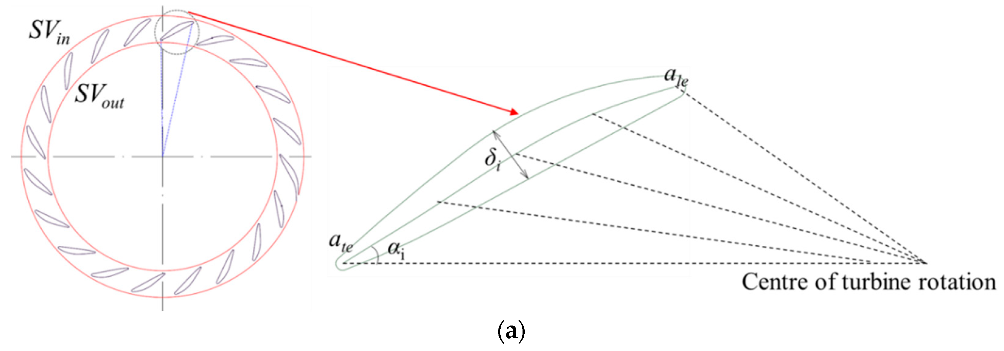
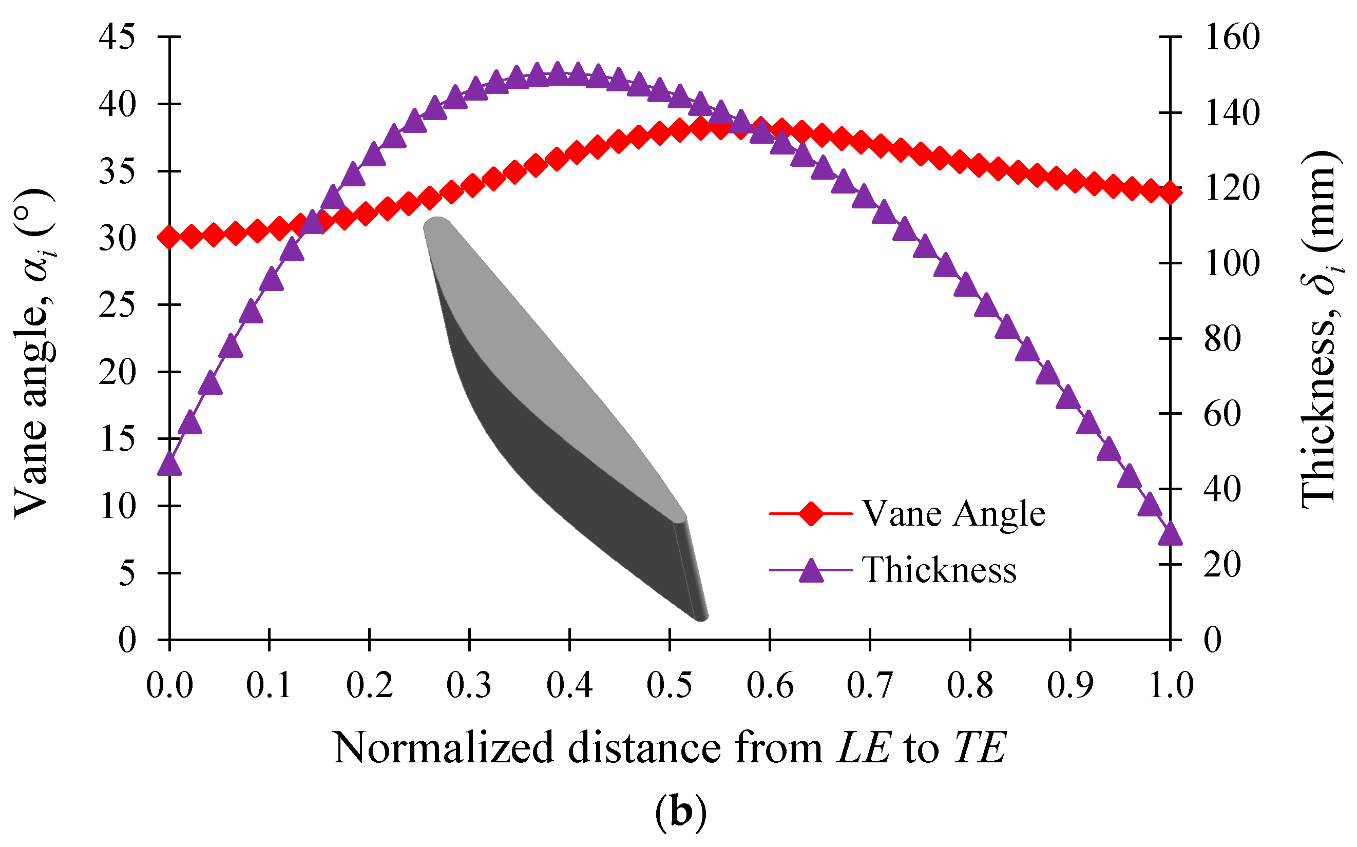
Processes 08 01392 g002aProcesses 08 01392 g002b
Figure 3. (a) Parametric design schematic view and (b) initial stay vane shape.
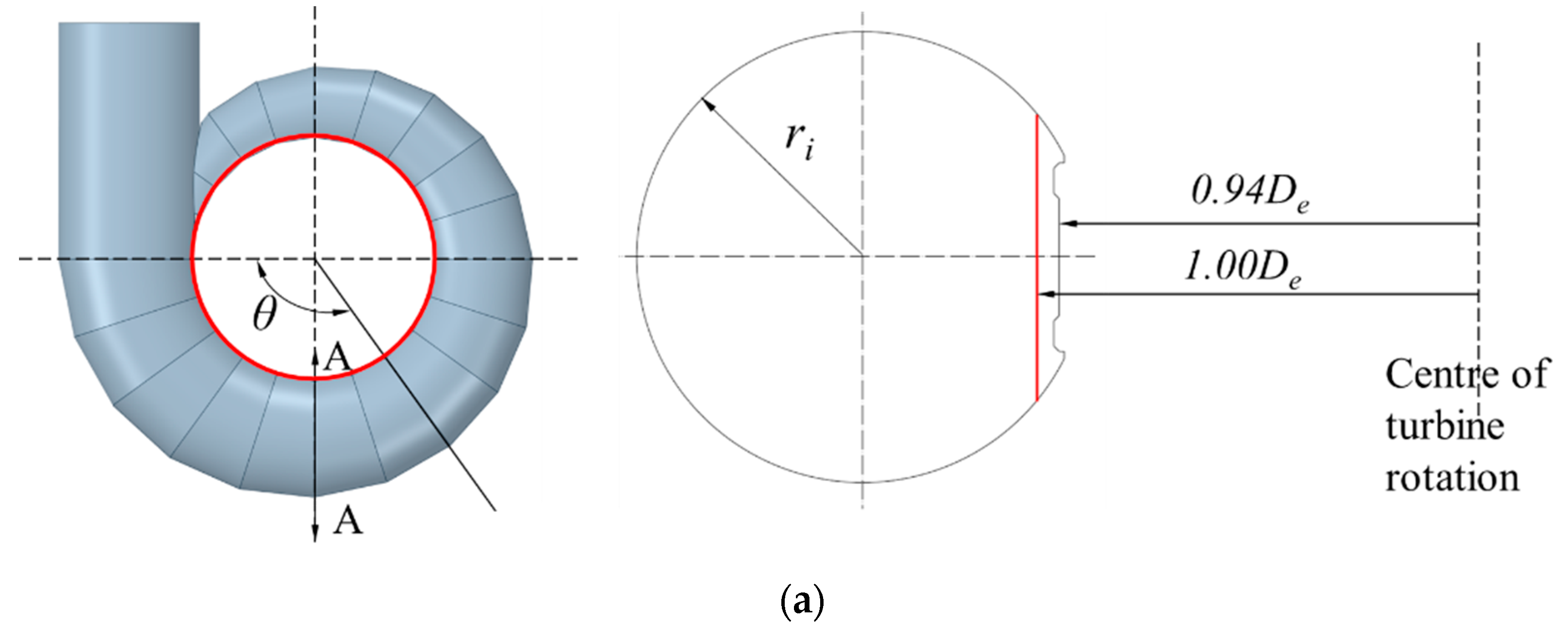
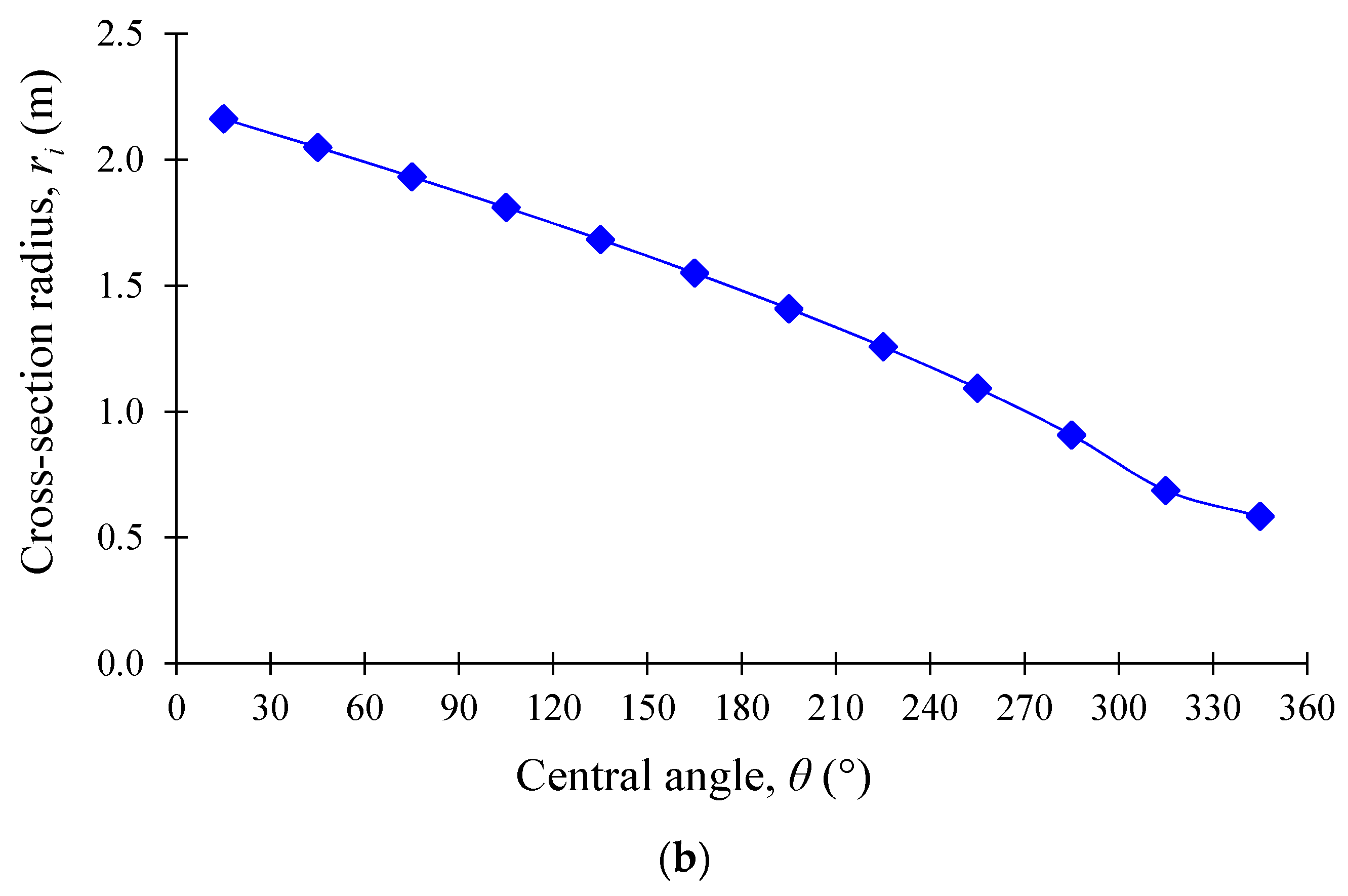
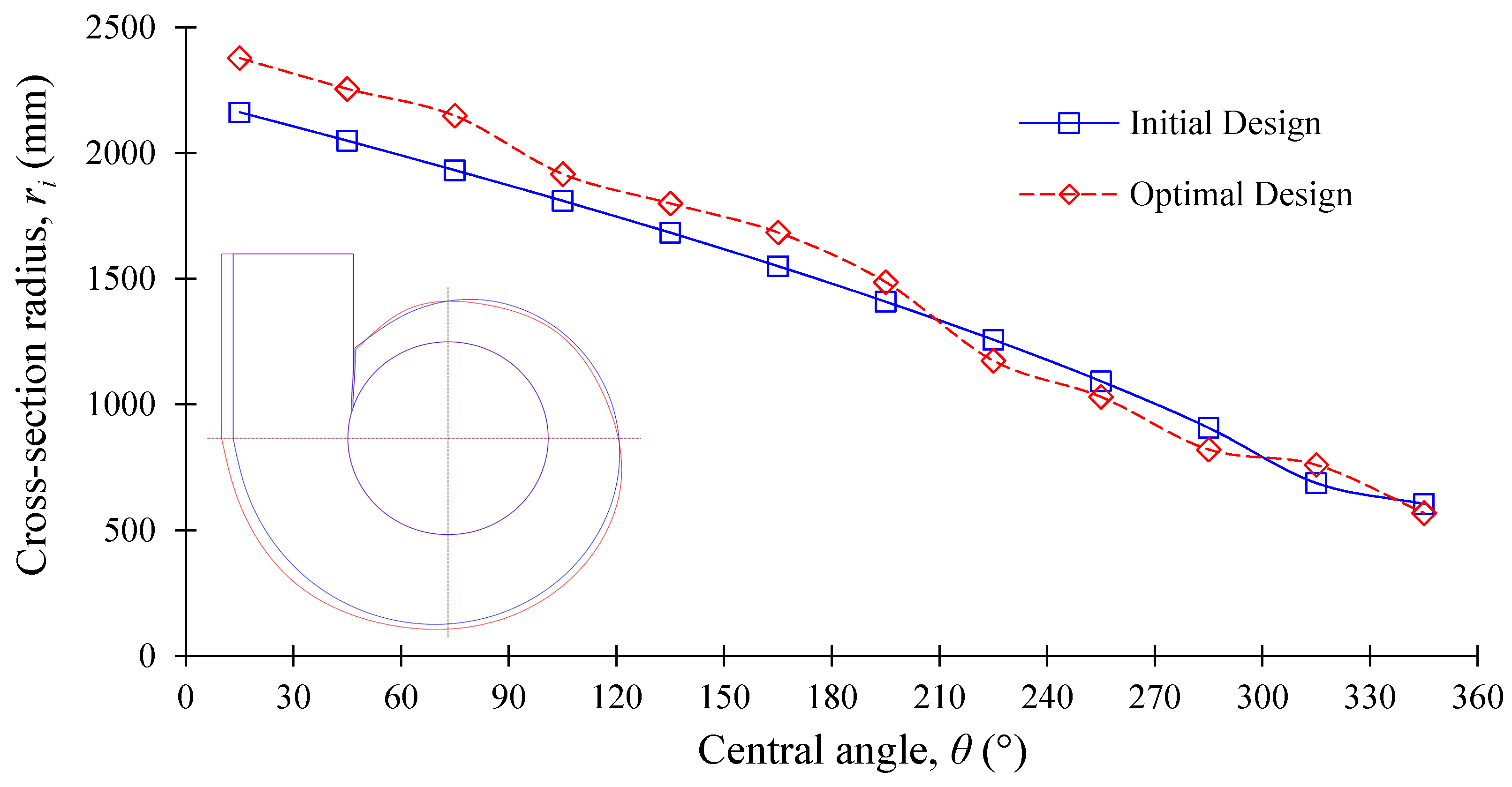
Processes 08 01392 g003aProcesses 08 01392 g003b
Figure 4. (a) Parametric design and (b) initial cross-section radius of casing (red line indicates measuring location).
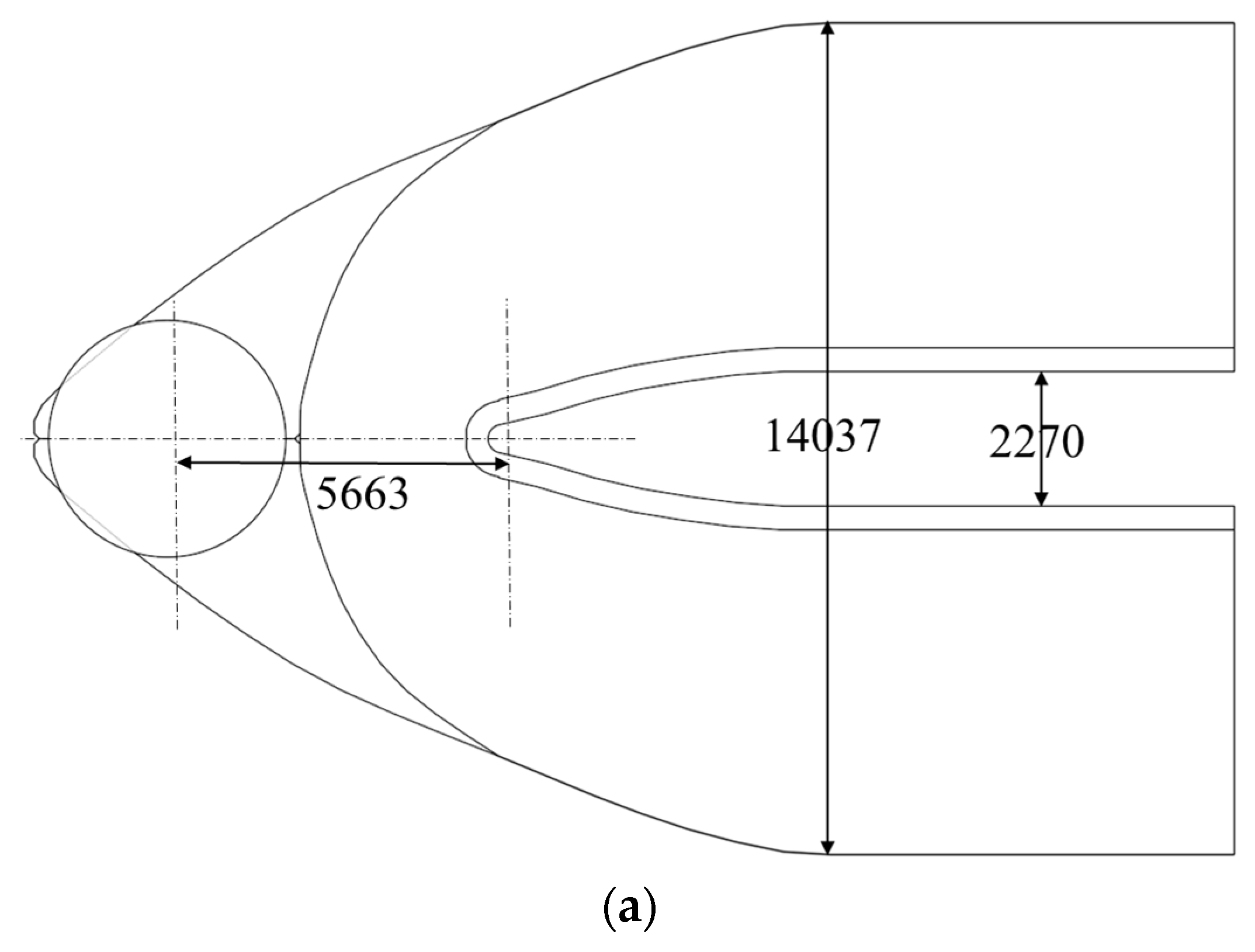
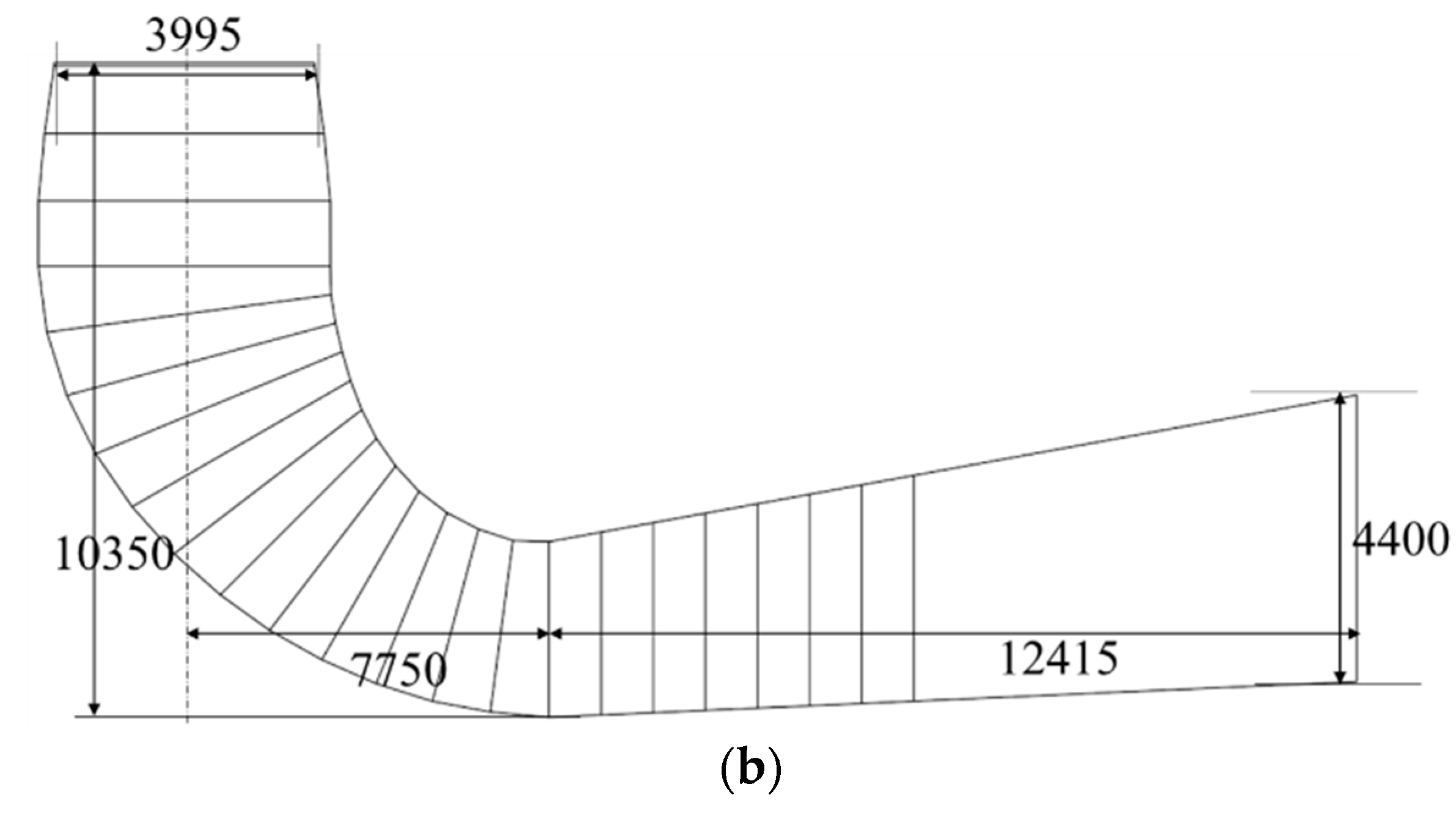
Processes 08 01392 g004aProcesses 08 01392 g004b
Figure 5. (a) Top view and (b) side view of draft tube (all dimensions are in mm).
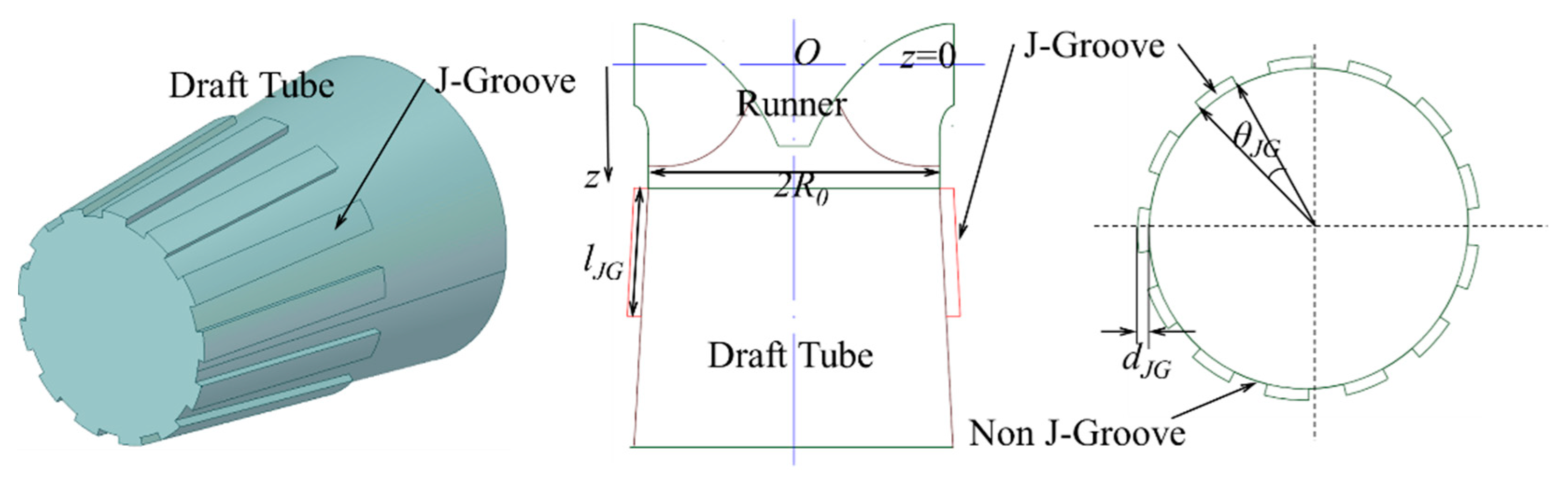
Processes 08 01392 g005aProcesses 08 01392 g005b
Figure 6. J-Groove shape install on the draft tube inner wall and design parameters.
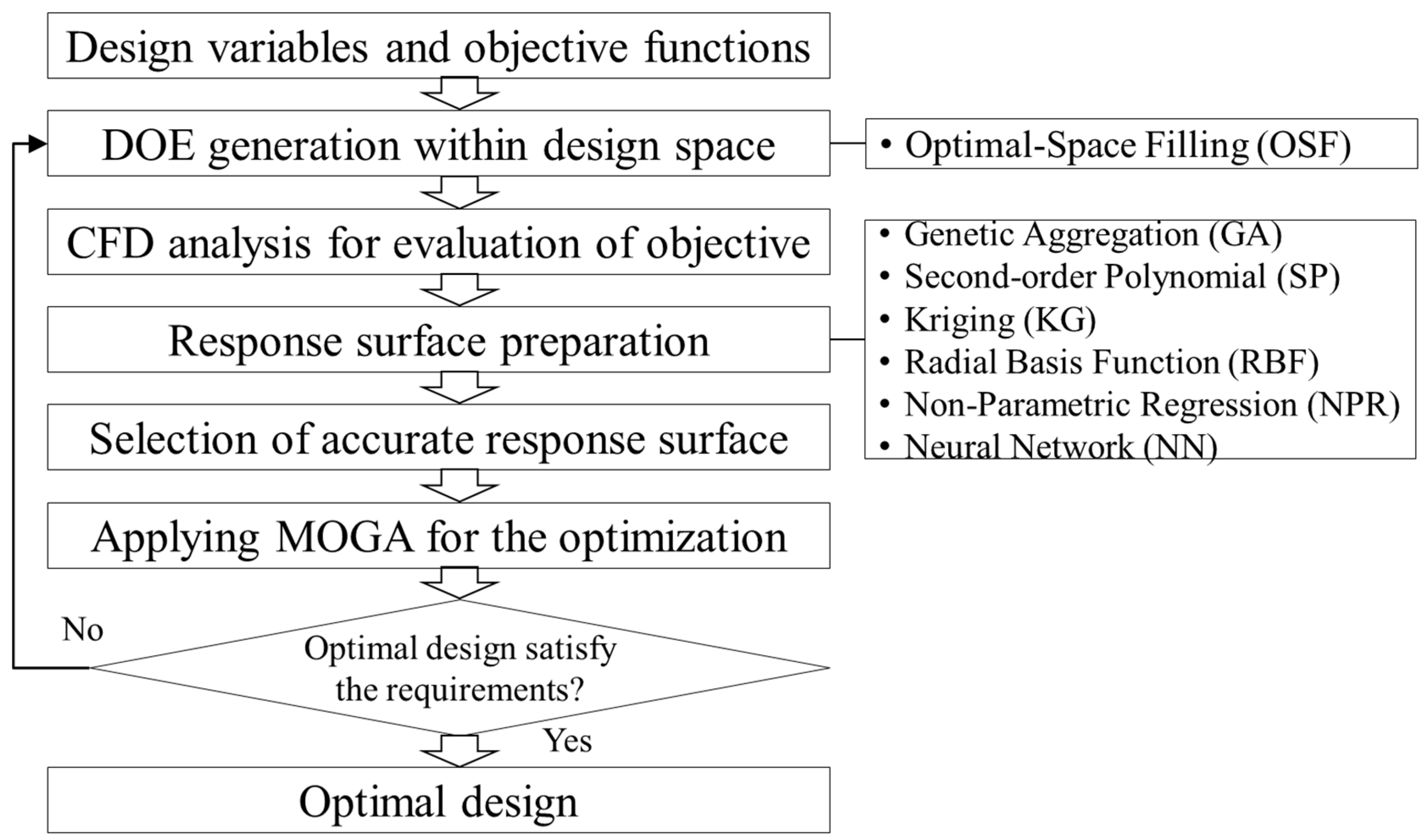
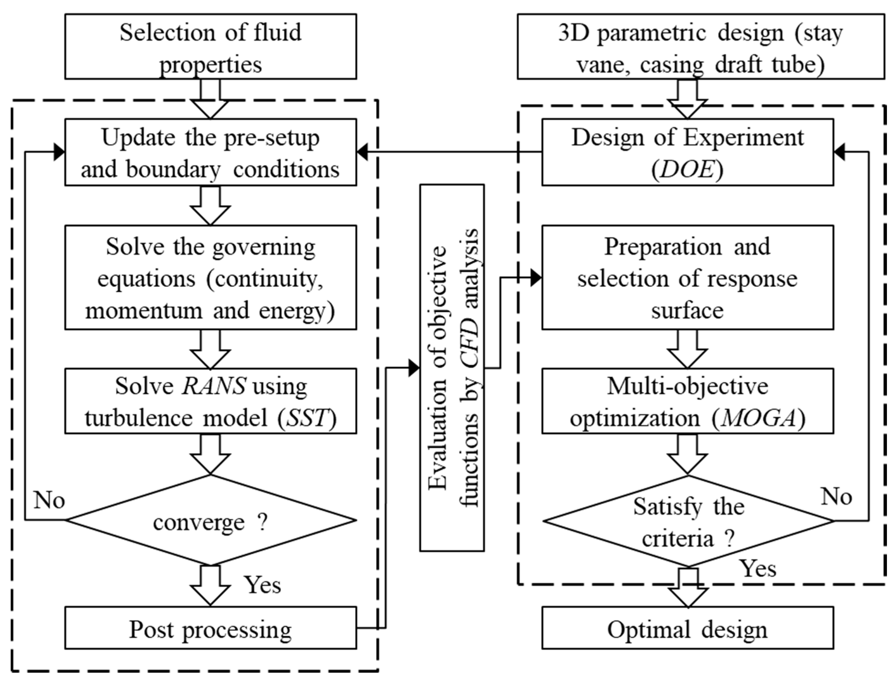
Processes 08 01392 g006
Figure 7. Optimization workflow for the 100 MW class Francis hydro turbine fixed flow passages. (DOE is Design of experiment and MOGA is Multi-Objective Genetic Algorithm).
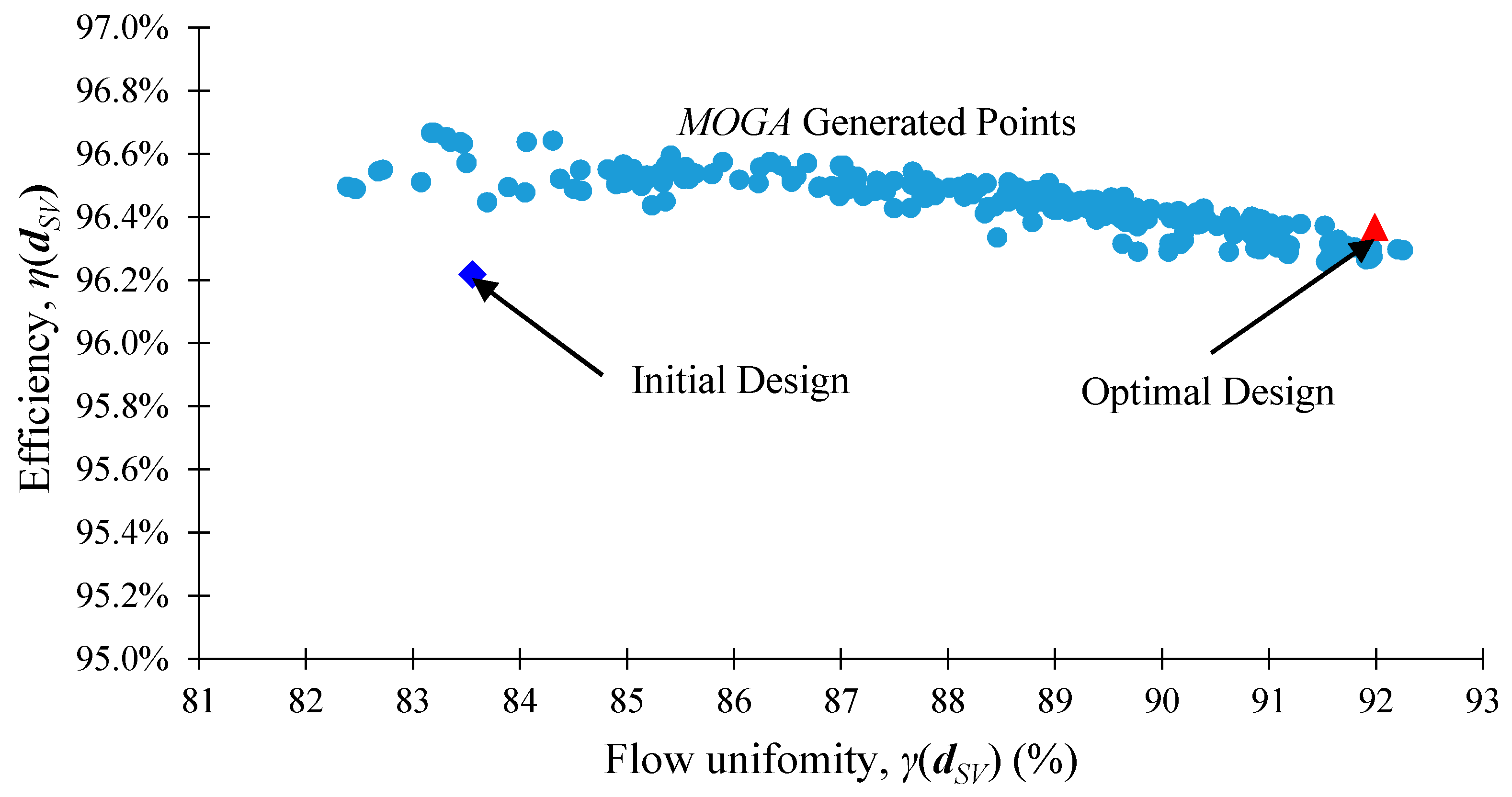
Processes 08 01392 g007
Figure 8. Pareto front for the optimization of stay vane design.
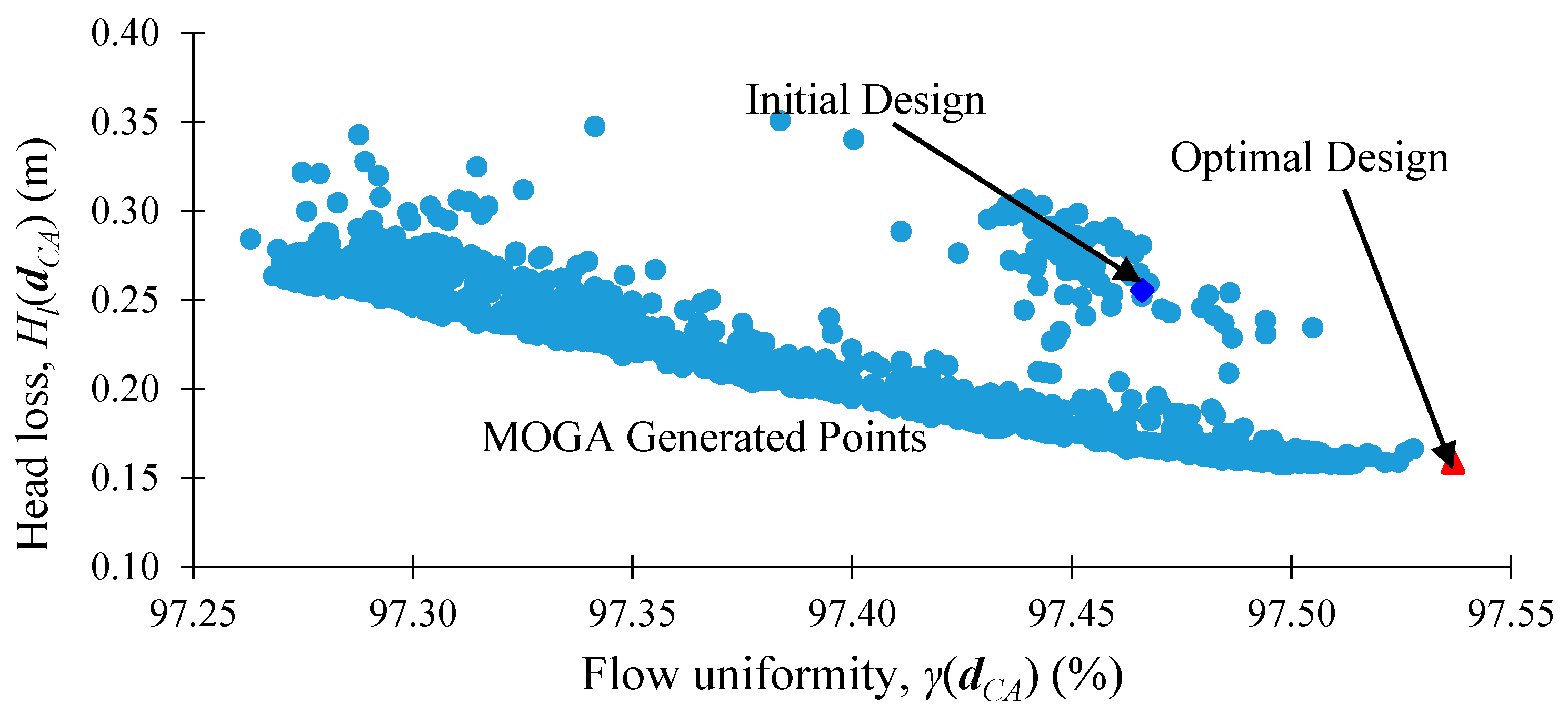
Processes 08 01392 g008
Figure 9. Pareto front for the optimization results of casing design.
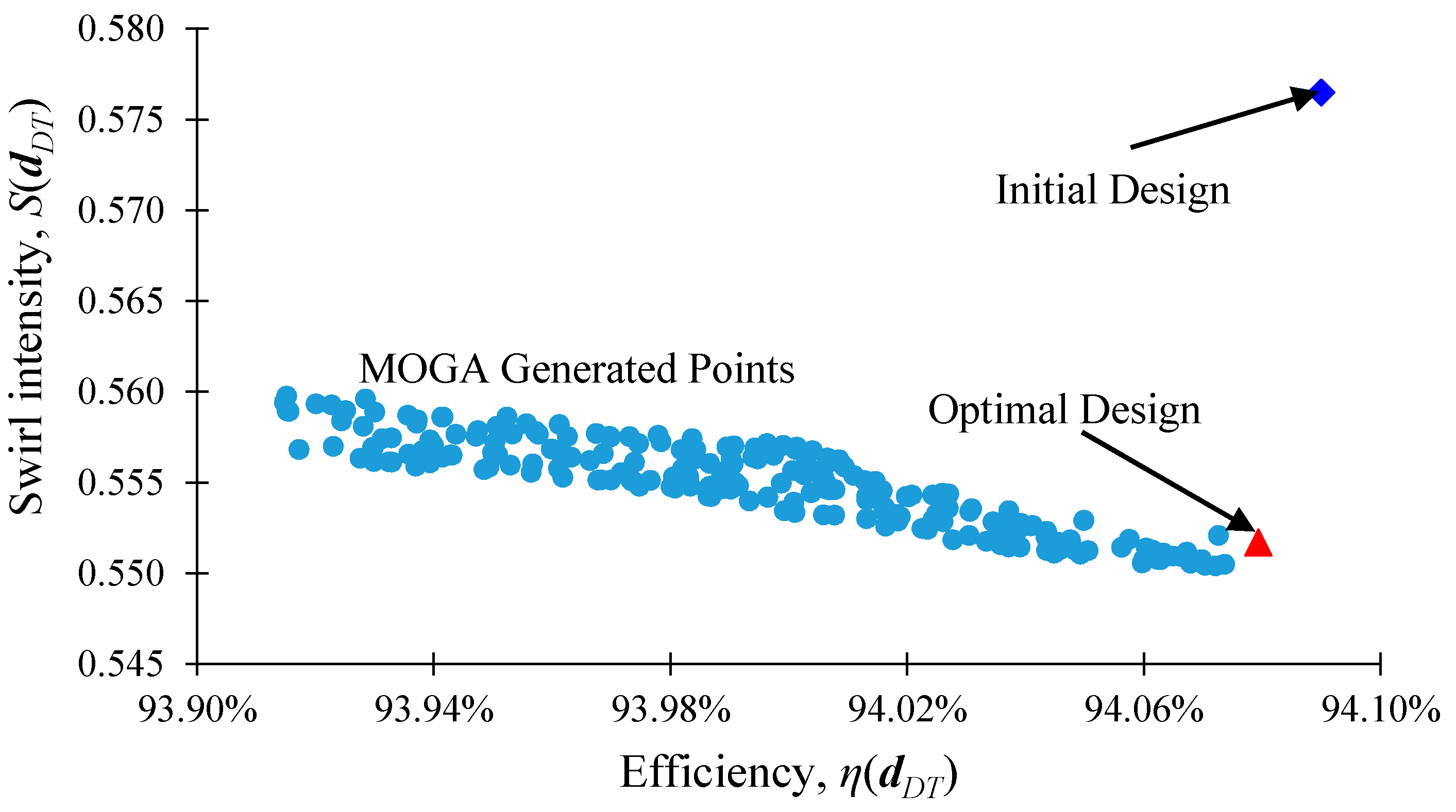
Processes 08 01392 g009
Figure 10. Pareto front for optimization of draft tube design at the design point.
Processes 08 01392 g010
Figure 11. Numerical scheme of CFD analysis in combination with optimal design process (RANS is Reynolds-averaged Navier-Stokes).
Processes 08 01392 g011
Figure 12. Numerical grids of the 100 MW class Francis turbine.
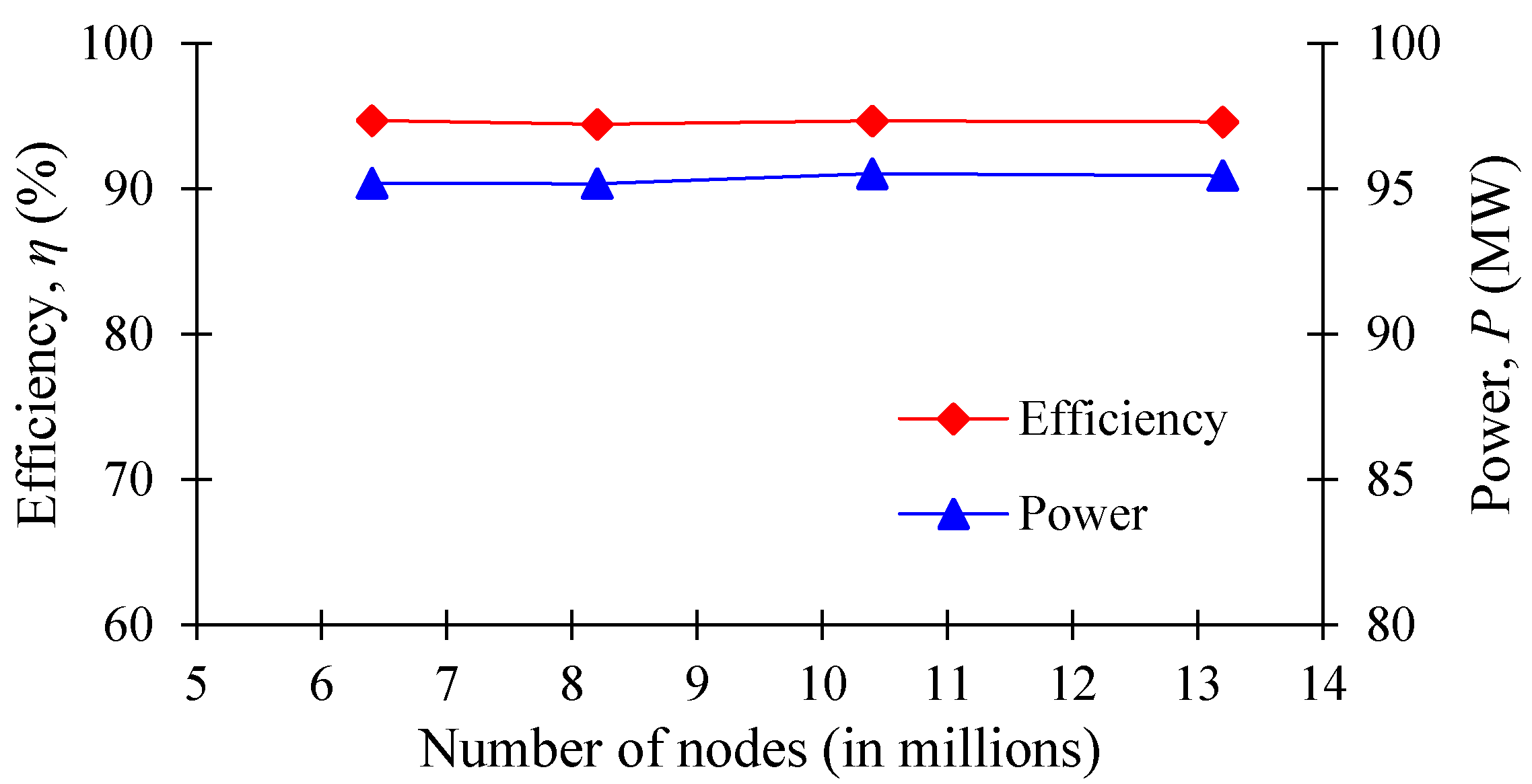
Processes 08 01392 g012
Figure 13. Mesh dependency test results for CFD analysis.
Processes 08 01392 g013
Figure 14. Validation of conceptual design of the 100 MW Francis hydro turbine by CFD analysis.
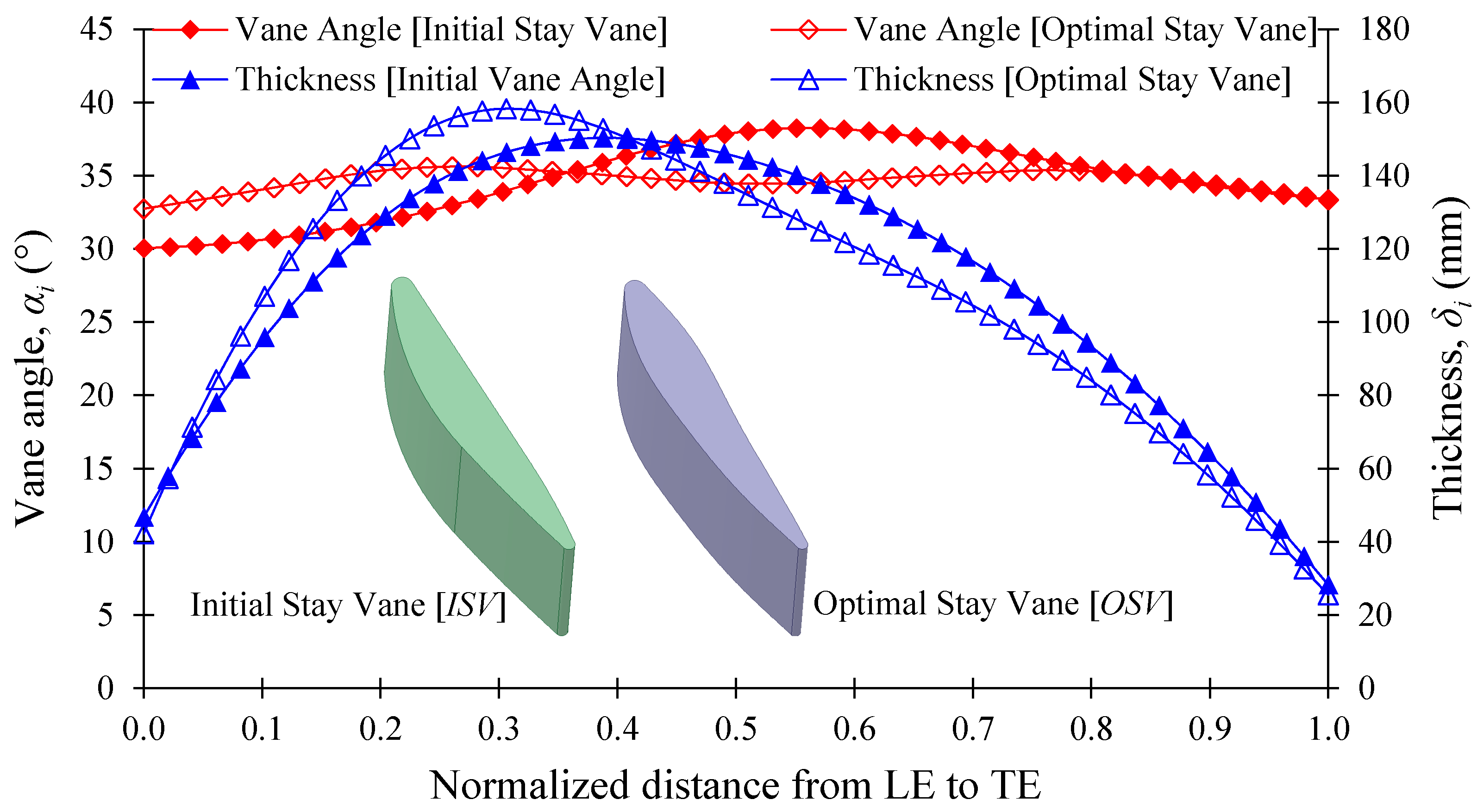
Processes 08 01392 g014
Figure 15. Comparison of initial and optimal stay vane designs for the 100 MW class Francis turbine.
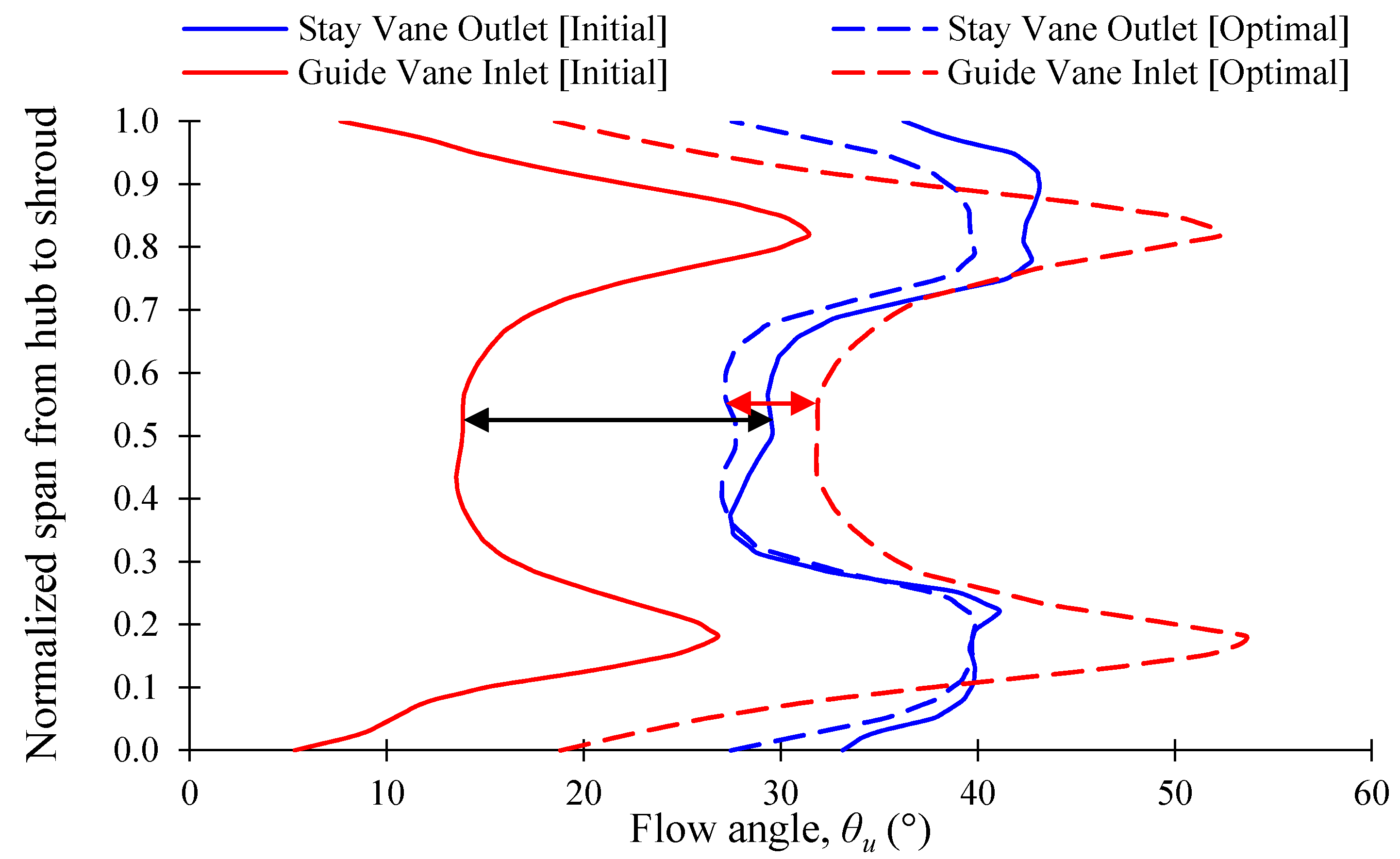
Processes 08 01392 g015
Figure 16. Comparison of flow angle in the ISV and OSV at the design point.
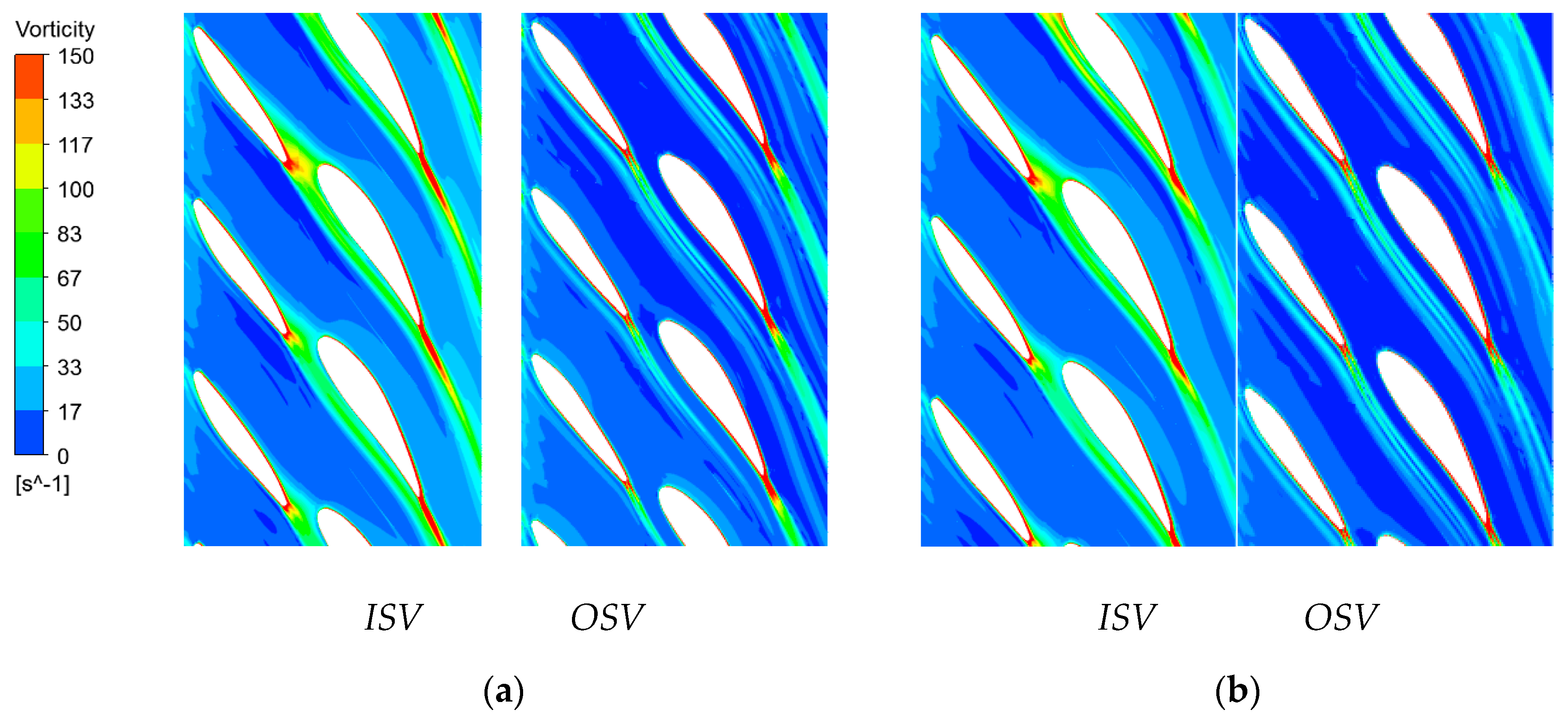
Processes 08 01392 g016
Figure 17. Comparison of vorticity in ISV and OSV flow passages (a) 0.25 span and (b) 0.75 span at design point.
Processes 08 01392 g017
Figure 18. Comparison of initial and optimal casing design for the 100 MW class Francis turbine.
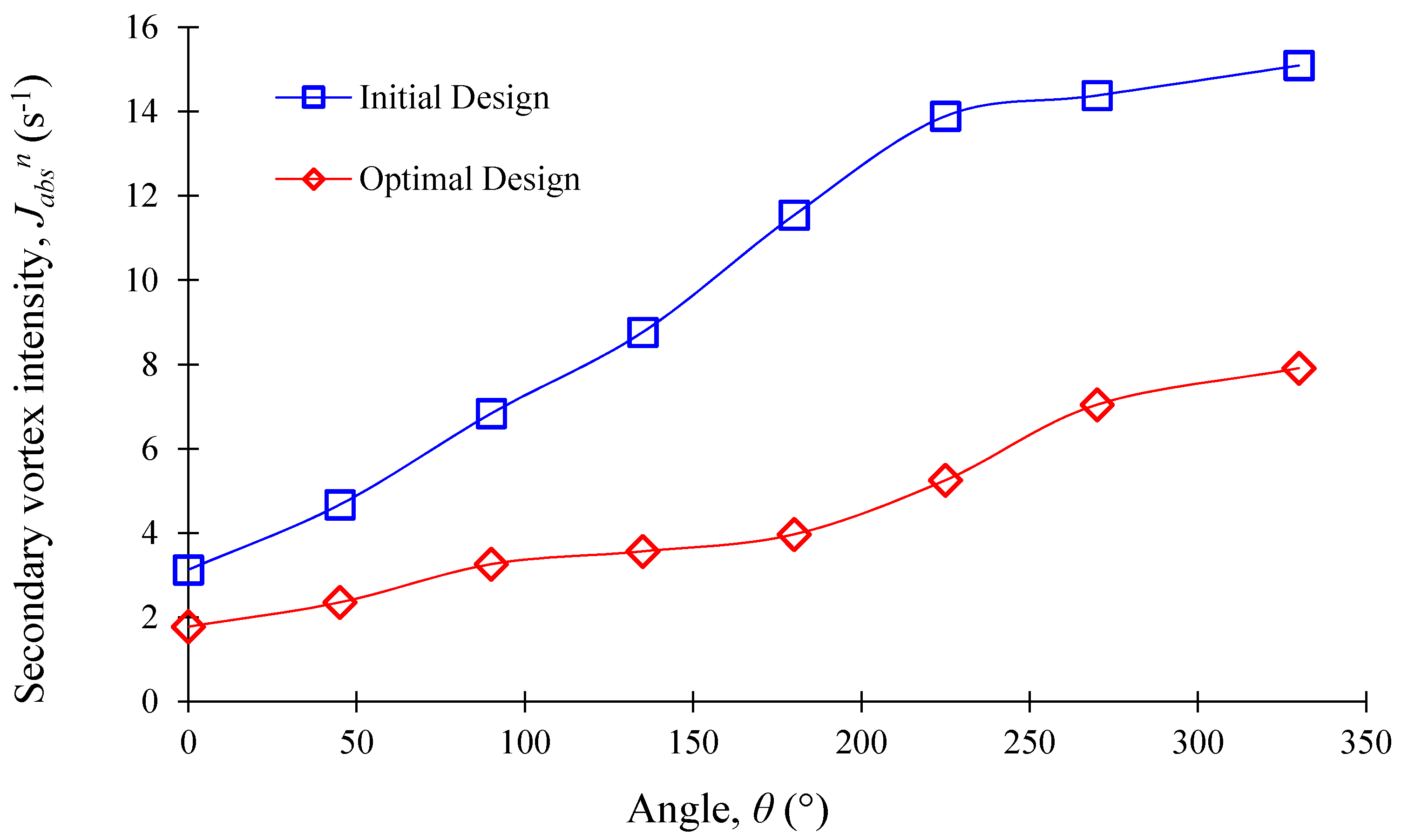
Processes 08 01392 g018
Figure 19. Comparison of secondary vortex intensity between initial and optimal casing designs.
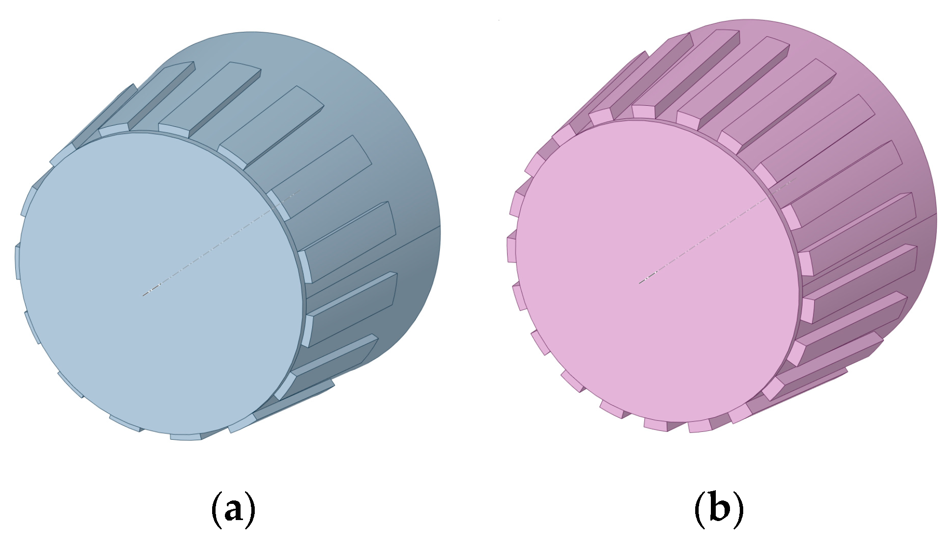
Processes 08 01392 g019
Figure 20. Comparison between (a) initial (b) optimal J-Groove models installed on the draft tube walls.
Processes 08 01392 g020
Figure 21. Comparison of swirl intensity in the draft tube by J-Groove shapes at the design point.
Processes 08 01392 g021
Table 1. Design specification of the 100 MW class Francis turbine.
NomenclatureUnitValues
Effective head, Hm90
Flow rate, Qm3/s125.4
Power, PMW100
Rotational speed, nmin−1180
Inlet diameter, Dimm4863
Outlet diameter, Demm3995
Specific speed, NskW-min−1-m205
Table 2. Results of goodness of fit test. (CoD is Coefficient of Determination, MRR is Maximum Relative Residual, RMSE is Root Mean Square Error).
Goodness MeasureRSMStay VaneCasingDraft Tube
η ( d S V ) γ ( d S V ) H l ( d S V ) γ ( d C A ) H l ( d C A ) η ( d J G ) S ( d J G ) H l ( d D T )
CoDGA98%97%90%98%98%100%97%99%
SP98%96%89%100%99%77%95%77%
KG100%100%100%100%100%100%100%100%
RBF100%100%100%100%100%100%100%100%
NPR99%99%100%100%100%100%100%100%
NN99%98%92%88%89%28%77%34%
MRRGA0.19%2.28%3.57%0.16%8.50%0.13%0.19%9.56%
SP0.10%3.04%35.74%0.13%31.20%0.11%0.69%16.65%
KG0.09%1.86%42.96%0.42%20.06%0.23%2.94%18.08%
RBF0.09%0.09%57.45%0.10%17.83%0.13%0.94%14.05%
NPR0.19%1.97%38.10%0.52%9.78%0.08%0.88%10.11%
NN0.15%1.47%28.3%0.54%20.13%0.05%0.65%6.17%
RMSEGA0.01%0.51%0.02%0.03%1.46%0.01%0.02%0.01%
SP0.01%1.36%0.04%0.13%31.20%0.01%0.06%0.02%
KG0.01%0.89%0.05%0.42%20.06%0.06%0.09%0.07%
RBF0.01%0.06%0.04%0.10%17.83%0.01%0.06%0.01%
NPR0.02%1.37%0.04%0.38%7.54%0.01%0.06%0.01%
NN0.01%0.82%0.03%0.35%16.51%0.03%0.04%0.01%
Table 3. Information of setting criteria for MOGA.
ParameterValue
Number of initial samples300
Maximum number of cycles30
Number of samples per cycle100
Crossover probability0.95
Mutation probability0.05
Maximum allowable Pareto percentage97
Convergence stability percentage2
Table 4. Bounds for design variables of stay vane.
Design Variable Lower   Bound   ( d S V L ) Upper   Bound   ( d S V U )
α126°32°
α229°36°
α334°42°
α432°39°
α530°36°
δ140 mm52 mm
δ2120 mm155 mm
δ3135 mm155 mm
δ495 mm120 mm
δ525 mm35 mm
ale, ate0.71.25
Table 5. Bounds for design variables of casing.
Design Variable Lower   Bound   ( d C A L ) Upper   Bound   ( d C A U )
r01900 mm2400 mm
r11800 mm2300 mm
r21700 mm2200 mm
r31600 mm2000 mm
r41500 mm1900 mm
r51350 mm1750 mm
r61250 mm1600 mm
r71100 mm1400 mm
r8950 mm1250 mm
r9800 mm1000 mm
r10600 mm800 mm
r11500 mm700 mm
Table 6. Bounds for design variables of draft tube shape.
Design Variable Lower   Bound   ( d D T L ) Upper   Bound   ( d D T U )
dJG50 mm200 mm
θJG20°
lJG1500 mm3000 mm
n J G 921
Table 7. Numerical grids information.
ComponentsNode NumberMesh Size (mm)Y + Value
Casing435,9227.529.5
Stay Vane1,561,2202.522.9
Guide Vane2,520,0003.034.3
Runner2,294,5955.084.2
Draft Tube1,428,8359.014.4
Total8,240,572
Table 8. Summary of boundary conditions for CFD analysis.
Parameter/BoundaryCondition/Value
InletTotal Pressure
OutletStatic Pressure
Rotational speed180 min−1
Turbulence modelShear Stress Transport (SST)
Grid interface connectionGeneral Grid Interface (GGI)
Physical time scaleSteady State/0.0531 s
Time stepUnsteady State/0.00185 s (2° per time step for 1 revolutions)
Interface modelSteady State/Frozen rotor Unsteady State/Transient rotor stator
WallsNo slip wall (roughness: smooth)
Table 9. Results of stay vane optimization for the 100 MW class Francis turbine.
ParameterInitial Stay Vane (ISV)Optimal Stay Vane (OSV)
Head (m)89.2389.23
Flow Rate (m3/s)130.36130.64
Power (MW)106.95107.23
Efficiency (%)93.9193.96
Flow Uniformity (%)91.7395.04
Head Loss (m)0.4380.403
Table 10. Results of casing optimization for the 100 MW class Francis turbine.
ParameterInitial DesignOptimal Design
Flow Uniformity (%)97.4697.51
Head Loss (m)0.2560.145
Table 11. Comparison of design parameter size of J-Grooves for draft tube shape optimization.
Design Parameter of J-GrooveInitial SizeOptimal Size
Length, lJG (mm)20002455.5
Depth, dJG (mm)106169
Angle, θJG (°)128.7
Number, n J G 1521
Table 12. Summary of draft tube shape optimization results for the 100 MW class Francis turbine.
ParametersWithout J-GrooveInitial J-GrooveOptimal J-Groove
Head (m)88.4188.4088.42
Flow Rate (m3/s)125.4125.53125.50
Power (MW)102.16101.79102.1
Efficiency (%)94.1294.0994.08
Swirl Intensity Reduction (%) at z/R0 = 2.25 12.1218.79
Publisher’s Note: MDPI stays neutral with regard to jurisdictional claims in published maps and institutional affiliations.

