Rapid Multi-Objective Optimization of Periodically Operated Processes Based on the Computer-Aided Nonlinear Frequency Response Method

Abstract

The dynamic optimization of promising forced periodic processes has always been limited by time-consuming and expensive numerical calculations. The Nonlinear Frequency Response (NFR) method removes these limitations by providing excellent estimates of any process performance criteria of interest. Recently, the NFR method evolved to the computer-aided NFR method (cNFR) through a user-friendly software application for the automatic derivation of the functions necessary to estimate process improvement. By combining the cNFR method with standard multi-objective optimization (MOO) techniques, we developed a unique cNFR–MOO methodology for the optimization of periodic operations in the frequency domain. Since the objective functions are defined with entirely algebraic expressions, the dynamic optimization of forced periodic operations is extraordinarily fast. All optimization parameters, i.e., the steady-state point and the forcing parameters (frequency, amplitudes, and phase difference), are determined rapidly in one step. This gives the ability to find an optimal periodic operation around a sub-optimal steady-state point. The cNFR–MOO methodology was applied to two examples and is shown as an efficient and powerful tool for finding the best forced periodic operation. In both examples, the cNFR–MOO methodology gave conditions that could greatly enhance a process that is normally operated in a steady state.

1. Introduction

1.1. Dynamic Process Intensification and Forced Periodic Operation Analysis

The idea of intensifying a process by switching from a steady-state (SS) to a forced periodic (FP) operation was first introduced by Douglas and Rippin in 1966 [1], and it was further expanded by Douglas [2], Horn and Lin in 1967 [3], and Bailey and Horn in 1971 [4]. Though in the beginning, the investigations of FP operations were limited to theoretical studies, in the next 25 years, there were at least 29 different experimental dynamic process intensification (PI) investigations of industrially important processes [5]. The initial investigations studied the FP operations with the modulation of one input variable: the inlet flow rate or the chemical composition (reactant concentration). The studies focused on enhancing the reaction rate, selectivity, and product distribution [5]. However, except for the reverse flow reactors, no remarkable improvements, i.e., process enhancements, were achieved by applying PI concepts in the time-domain. This was the case until the emergence of sophisticated process system engineering (PSE) techniques and methods that were mostly used for PI in multi-functional units [6].

The surge of the computer industry at the end of the 20th century and the use of advanced numerical solvers and new algorithms had a great impact in the area of chemical engineering and led to new PI concepts in the field of process synthesis and design [7]. Different dynamic single-objective optimization (SOO) techniques were available for research on a plant-level [8] and the optimization of processes on a unit-level (e.g., reactor operation) [9,10,11,12,13,14].

For optimizing periodic operations in chemical engineering, a variety of different numerical methods have been introduced [11,14,15,16,17,18,19,20,21,22]. Most methods, in the beginning, were single-objective optimization algorithms that computed the time-average performance of a process [15,16]. Dynamic optimization methods, which were very suitable for the optimization of periodic processes, allowed users to find an optimal solution around a predefined SS point and rely on local optimization algorithms [11]. In cases where there were many different possibilities regarding the modulated inputs and no fast and accurate way of calculating time-average performance, the dynamic local SOO proved to be time-consuming, numerically expensive, and inaccurate (far from the global optimum), leading to only marginal process improvements [14]. As Özgülşen et al. pointed out, the most challenging difficulty in determining optimal parameter values in forced periodic operations was locating the global maximum [15]. The use of global optimization methods would remove this difficulty, and further advances would eliminate the need for initialization strategies to solve nonlinear programming problems [7].

Recently, Rangaiah et al. [23] published a review and tutorial of a five-step procedure used to create, solve, and select the optimal results of chemical engineering problems using multi-objective optimization (MOO). One of the most widely used MOO algorithms for the optimization of engineering problems is the non-dominated sorting hybrid algorithm [24]. In the last five years, there has been a significant usage of MOO in chemical engineering [25,26,27,28,29,30,31,32,33]. The advantage of MOO over SOO is that it allows for a multi-criteria analysis for choosing the best solution [26]. Additionally, MOO does not depend on user-supplied initialization procedures. However, not many examples can be found where global dynamic SOO or MOO were used for the optimization of FP operation with modulation of several input variables [11,14].

As Baldea and Edgar pointed out [34], although dynamic PI (FP operation) can significantly enhance process performance, several hurdles still need to be overcome:

• A systematic framework for the identification of possible dynamically intensified processes is required.
• Various mathematical and numerical challenges while optimizing and computing the cyclic processes need to be addressed.
• New techniques that encompass the previous points should be part of intuitive software tools that can be used both in academia and industry.

The idea of this research was to address the beforementioned challenges using a completely new approach based on an analytical PSE tool for predicting the time-average behavior of periodic processes—the Nonlinear Frequency Response (NFR) method [35]. Recently, this method was upgraded by developing a new PSE software application, leading to the so-called computer-aided Nonlinear Frequency Response (cNFR) method [36].

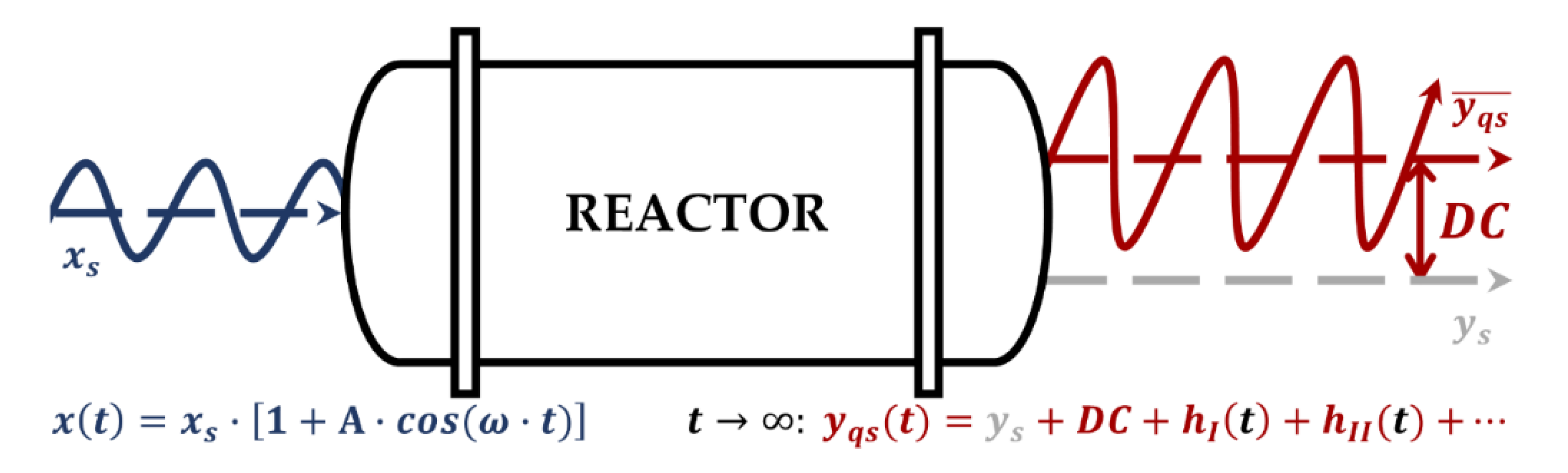
1.2. The NFR Method for Evaluating the Potential of Process Intensification through Forced Periodic Operations

The Nonlinear Frequency Response (NFR) method is an analytical PSE tool based on the concept of higher-order frequency response functions (FRFs) [37]. The NFR method allows users to transfer a dynamic mathematical model of a weakly nonlinear system from the time domain to the frequency domain. In the frequency domain, the system is mathematically represented with a set of the first, second, and higher-order FRFs [37], which are functions of frequency. Though an infinite sequence of FRFs is needed for full representation of the system, it was shown that good approximations can be achieved by using only the first and second-order FRFs [38].

For an easier understanding of the NFR method, Figure 1 shows a schematic representation of a chemical reactor with forced, sinusoidal modulation of an input $x$ around its SS value $x_s$. For a stable system, after going through a transient, any output from the reactor will eventually reach a quasi-(periodic)-steady-state $y_{qs}$. Most processes in chemical engineering, including chemical reactors, are weakly nonlinear (all nonlinear terms in their model equations are continuous and differentiable, i.e., can be represented in the Taylor series form). The NFR method can only be applied to stable, weakly nonlinear systems that can be represented with convergent Volterra series. Another limitation is that the analyzed systems must not have multiple steady states. For such systems, the quasi-steady- state of the response is obtained as a sum of its SS value, the first harmonic (of the same frequency as the input), a theoretically indefinite number of higher harmonics, and a nonperiodic term (the so-called DC component), as shown in Figure 1. The DC component represents the difference between the time-average of the output in the FP regime and its SS value and is the measure of PI owing to the FP operation.

The NFR method based on the concept of higher-order frequency response functions (FRFs) [39] enables the fast and easy estimation of the DC component. For the sinusoidal modulation of a single input $x$, with amplitude $A$ and frequency $\omega$, the DC component can be approximately evaluated by using only the asymmetrical second-order FRF $G_{x,y}^{\left(2\right)}\left(\omega ,-\omega \right)$ relating the output $y$ and input $x$:

$$D{C}_{x,y}\approx 2·{\left(\frac{A}{2}\right)}^2·G_{x,y}^{\left(2\right)}\left(\omega ,-\omega \right)$$

(1)

The sign of $D{C}_{x,y}$, which is the same as the sign of $G_{x,y}^{\left(2\right)}\left(\omega ,-\omega \right)$, answers whether the FP operation would result in process improvement or not, while its value gives a very good estimate of the extent of the improvement.

When two input signals ($x_1$ and $x_2$) are modulated, with amplitudes $A_1$ and $A_2$ and a phase angle $\phi$ between them, then:

$$x_1\left(t\right)=x_{1,s}·\left[1+A_1·cos\left(\omega ·t\right)\right]$$

(2)

$$x_2\left(t\right)=x_{2,s}·\left[1+A_2·cos\left(\omega ·t+\phi \right)\right]$$

(3)

the DC component can be approximately calculated as a sum of contributions of the inputs $x_1$ and $x_2$, separately, and the contribution of their cross-effect [40]:

$$\begin{gathered} D{C}_{x1x2,y}\approx 2·{\left(\frac{A_1}{2}\right)}^2·G_{x1,y}^{\left(2\right)}\left(\omega ,-\omega \right)+2·{\left(\frac{A_2}{2}\right)}^2·G_{x2,y}^{\left(2\right)}\left(\omega ,-\omega \right)+ \\ 2·\left(\frac{A_1}{2}\right)·\left(\frac{A_2}{2}\right)·\left\{\cos \phi ·Re\left[G_{x1x2,y}^{\left(2\right)}\left(\omega ,-\omega \right)\right]+\sin \phi ·Im\left[G_{x1x2,y}^{\left(2\right)}\left(\omega ,-\omega \right)\right]\right\} \end{gathered}$$

(4)

where $G_{x1x2,y}^{\left(2\right)}\left(\omega ,-\omega \right)$ is the cross asymmetrical second-order FRF. From Equation (4), it follows that the simultaneous modulation of two inputs has a higher PI potential in FP operations than single-input modulations (Equation (1)), as the sign of the cross-term can be easily adjusted by correctly selecting $\phi$ [40]. Due to this, by modulating the system with two inputs with an optimal phase difference, improvements become possible even in cases when modulating one or both inputs, separately, leads to process deterioration [41].

The NFR method is a PSE tool for the fast and easy prediction of the approximate time-average values of the outputs of interest (as shown in Equations (1) and (4)). Even though the NFR method gives an approximate value of the DC component, it has been shown that good estimates can be achieved by using only the second-order asymmetrical FRFs (Equations (1) and (4)) [35,39,40,41,42,43,44,45,46,47,48,49]. Thus far, the NFR method has been used for the dynamic PI analysis of isothermal [39,40,42] and nonisothermal [41,43,44,45,46,47] reactors with sinusoidal [39,40,41,42,43,45,46,49] or other periodic shapes [44,50] of the modulated inputs.

It is important to note that different performance criteria of interest (e.g., conversion, yield, selectivity, and productivity) of FP operation can be directly calculated from the time-average values of the outputs obtained using the NFR method. Using Equations (1) and (4), they can be expressed in the algebraic form as functions of the input modulating parameters (frequency, amplitudes, and phase shift).

One of the most important steps of applying the NFR method is the derivation of the needed FRFs. Though the procedure for the analytical derivation of FRFs is well-established and has been used and presented in many publications [35,39,40,41,43,44,45,46,47,48,49,50,51,52,53,54], it is rather complex, time-consuming, and requires certain mathematical skills in the complex domain. As such, the NFR method can be unappealing to beginners, especially when applied to more complex systems.

The recently developed computer-aided Nonlinear Frequency Response (cNFR) method [36] is an upgrade of the NFR method using a software application for the automatic derivation of the FRFs of interest. It has an easy-to-use interface where the user can define the dynamic model equations of the system and automatically generate MATLAB files for the desired FRFs and DC components [36]. The generated MATLAB files contain codes with algebraic expressions of the derived FRFs and DC components in the vector form, and they enable very fast simulation of the key system performance criteria and rapid rigorous global and local optimization. No time-consuming and numerically expensive methods are required for solving the systems of differential equations. In this way, the cNFR method provides answers to three key questions about the potential of the investigated FP operation:

• Which input or combination of inputs should be periodically modulated?
• What are the optimal forcing parameters of the modulated inputs: frequency, amplitudes, or phase shift ($\omega , A_1$ and $A_2$, or $\phi$, respectively)?
• What is the expected process improvement if we switch from SS to FP operation (a maximal increase in the performance criteria of interest)?

By giving answers to these questions in a fast and easy manner, the cNFR method overcomes most challenges listed by Baldea and Edgar. As is shown in this paper, the cNFR method has the potential to become a very strong software PSE tool for analyzing the dynamic PI potential.

The cNRF software tool was explained in detail by Živković et al. [36]. Thus far, it was used for the analysis of the FP operation of an isothermal continuous stirred tank reactor (CSTR) with the simultaneous modulation of feed concentration and flow-rate [24], for experimental identification [55], and for the evaluation of the FP operation of an electrochemical process [41].

In this work, a new methodology for the rigorous multi-objective optimization (MOO) of forced periodic (FP) operations is presented. It is based on the cNFR method and cost–benefit indicator analysis.

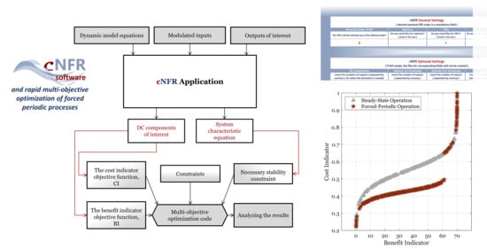
2. The cNFR–Multi-Objective Optimization Methodology for Periodically Operated Processes

In Figure 2, the cNFR–MOO methodology is shown schematically. It consists of steps done by the user (gray rectangles) and stages that are a direct result of the application of the cNFR software tool (white rectangles). Explanations of how the dynamic model equations, modulated inputs, and outputs of interest are defined is given in a publication by Živković et al. [36], where the cNFR tool was presented. After using the cNFR tool, in a matter of minutes, the user gets automatically generated MATLAB files that contain all FRFs, DC components of interest, and a system characteristic equation that can be used for the determination of system stability (Figure 2).

System stability is an important prerequisite for the use of the cNFR method [36] and should be used as one of the algebraic constraints in MOO. The system is stable as long as all roots of the characteristic equation derived by the cNFR method remain negative [36]. Therefore, this necessary stability constraint (Figure 2) is already provided as a function to the user and should be included in the MOO code. Other constraints can also be defined if needed.

The objective functions reflect important system criteria (e.g., reactor capacity, productivity, and selectivity) and can differ from case to case. In general, a cost indicator (CI) is set as a combination of the DC components of system variables that are undesired and expensive from the process point of view. On the contrary, the benefit indicator (BI) is defined as a combination of the DC components of the most beneficial variables in the system. An objective function can also contain a combination of both BIs and CIs. MOO constraints and objective functions expressed through CIs and BIs are defined in the MATLAB code by the user (Figure 2). The main reason that MOO is preferred over SOO is that it enables users to examine multiple optimal solutions for different values of competing objective functions of interest. Additionally, it provides results in cases where SOO can lead to mathematically infinite ($\underset{CI\to 0}{\lim }\frac{1}{CI}$, $\underset{\begin{array}{c}BI\to \infty \\ CI\to 0\end{array}}{\lim }\frac{BI}{CI}$, etc.) or undefined results ($\underset{\begin{array}{c}BI\to 0\\ CI\to 0\end{array}}{\lim }\frac{BI}{CI}$, $\underset{\begin{array}{c}CI1\to \infty \\ CI2\to 0\end{array}}{\lim }\left(CI1·CI2\right)$, etc.) [25].

It is important to point out that in the cNFR–MOO methodology, we optimize the steady-state (SS) and forcing parameters all in one step. This is different than in classical approaches of optimizing periodic operations, which are usually performed in two steps: first by finding the optimal SS point and then by finding the optimal forcing parameters (frequency, amplitudes, and phase shift) of the input modulations around that SS. The reason for simultaneous optimization of SS and forcing parameters is that the DC component—defining the process improvement—depends on the SS values of the process variables, and it is possible that perturbing the system around a sub-optimal instead of an optimal steady state can result in higher improvements. Thus, it is possible to find a periodic operation that gives the best possible results regarding the chosen performance criteria. As a result of such optimization, a complete set of parameters is obtained: the SS point and the forcing parameters of the modulated inputs.

The final step shown in Figure 2 consists of results analysis and additional FRF and DC component simulations if the further evaluation and understanding of the FP operation are needed. The cNFR method is applied to MOO in Section 3 on two examples: (1) an isothermal continuous stirred tank reactor (CSTR) with a simple reaction mechanism and (2) an electrochemical reaction (ECR) process.

3. Examples of the cNRF-Based Rapid Multi-Objective Dynamic Optimization

3.1. Example 1: Isothermal Continuous Stirred Tank Reactor with a Simple Reaction Mechanism (CSTR)

3.1.1. Problem Formulation

In Example 1, the following irreversible $n$-th-order reaction

$$A\stackrel{k_r}{\to }P$$

(5)

is taking place in an isothermal continually stirred tank reactor (CSTR) with a constant volume, where $A$ is the reactant, $P$ is the product, and $k_r$ is the rate constant of a simple $n$-th order reaction rate:

$$r=k_r·C_A{}^n$$

(6)

For an isothermal CSTR, only material balance equations are needed to fully mathematically describe the system:

$$V·\frac{d{C}_A\left(t\right)}{dt}=F\left(t\right)·C_{Ai}\left(t\right)-F\left(t\right)·C_A\left(t\right)-V·r\left(t\right)$$

(7)

$$V·\frac{d{C}_P\left(t\right)}{dt}=F\left(t\right)·C_P\left(t\right)+V·r\left(t\right)$$

(8)

where $t$ is time, $V$ is the volume of the reaction mixture, $F$ is the volumetric flow rate, $C_{Ai}$ is the reactant inlet concentration, and $C_A$ and $C_P$ are the outlet concentrations of reactant and product, respectively.

The molar flow rates for reactant inlet and product outlet can be expressed as:

$$M{F}_{Ai}\left(t\right)=F\left(t\right)·C_{Ai}\left(t\right)$$

(9)

$$M{F}_P\left(t\right)=F\left(t\right)·C_P\left(t\right)$$

(10)

This simple case was already used as an example for the analysis of potential PI by FP operations, first by using the standard NFR method [39,40] and then by the cNFR method [36]. Here, this example is used to illustrate MOO based on the cNFR method for finding the optimal periodic operation for the case of simultaneous sinusoidal modulations of the feed concentration $C_{Ai}$ and flow rate $F$:

$$C_{Ai}\left(t\right)=C_{Ai,s}·\left[1+A_1·\cos \left(\omega ·t\right)\right]$$

(11)

$$F\left(t\right)=F_s·\left[1+A_2·\cos \left(\omega ·t+\phi \right)\right]$$

(12)

where index s denotes the variable steady-state (SS) and $A_1$, $A_2$, and $\phi$ are forcing parameters. For the purposes of optimization, dimensional frequency, $\omega$, is used instead of the nondimensional, ${\omega }_{nd}$, according to the following equation:

$$\omega ={\omega }_{nd}·\frac{F_s}{V}$$

(13)

The optimal SS operation is used as a base case for comparison.

3.1.2. Formulation of the Objective Functions and Constraints

The two objective functions that are used are the maximized product yield $Y_P$ and the reactor volumetric capacity $\kappa$. For periodic operations with variable flow rates, these values are defined based on the time-average values of the inlet and outlet molar flow rates [43]:

$$\max \left(Y_P\right) \mathrm{where} Y_P=\frac{\overline{F\left(t\right)·C_P\left(t\right)}}{\overline{F\left(t\right)·C_{Ai}\left(t\right)}}=\frac{\overline{M{F}_P\left(t\right)}}{\overline{M{F}_{Ai}\left(t\right)}}$$

(14)

$$\max \left(\kappa \right) \mathrm{where} \kappa =\frac{\overline{F\left(t\right)·C_{Ai}\left(t\right)}}{V}=\frac{\overline{M{F}_{Ai}\left(t\right)}}{V}$$

(15)

By expressing the time-average outlet molar flow rate of the product, based on the corresponding DC component $D{C}_{F{C}_{Ai},M{F}_P}$, Equation (14) becomes [36]:

$$Y_P=\frac{M{F}_{P,s}}{F_s·C_{Ai,s}}·\frac{\left(1+D{C}_{F{C}_{Ai,M{F}_P}}\right)}{1+2·\frac{A_1}{2}·\frac{A_2}{2}·\cos \left(\phi \right)}$$

(16)

where the subscript $s$ denotes the SS values of the variables. Product yield (Equations (14) and (16)) is the first benefit indicator (BI1). The second benefit and also a cost indicator (BI2/CI) is the reactor volumetric capacity (Equation (15)), and its value is maximized to get a smaller reactor volume, as a cost indication, and higher capacity, as a benefit indication.

In the current analysis, the only constraint is that the system must be stable. As explained in our previous publications [36,40], the condition of the reactor stability can be expressed in the form of the following inequality:

$$-C_{A,s}·F_s-C_{A,s}{}^n·V·k_r·n<0$$

(17)

3.1.3. Optimization Variables and Criteria Formulation

In

Table 1. Pareto optimization variables for Example 1: CSTR and its corresponding lower and upper bounds with scaling values (in brackets).

Variable	SS Operation		FP Operation
	Lower Bound	Upper Bound	Lower Bound	Upper Bound
$F_s$, m3/min	1 × 10−12	1	1 × 10−12	1
$F_{Ai,s}$, kmol/m3	1 × 10−12 (×20)	1 (×20)	1 × 10−12 (×20)	1 (×20)
$V$, m3	0.01 (×100)	1 (×100)	0.01 (×100)	1 (×100)
$A_1$, /			0	1
$A_2$, /			0	1
$\omega$, rad/s			0 (×2π)	1 (×2π)
$\phi$, rad			0 (×2π)	1 (×2π)

CSTR: continuous stirred tank reactor; SS: steady-state; FP: forced periodic.

, the optimization variables for both the SS and FP operations are listed. The SS CSTR operation has only SS optimization variables, i.e., volumetric flow rate ($F_s$), inlet concentration ($C_{Ai,s}$), and the reaction mixture volume ($V$). On the other hand, the FP operation has additional dynamic optimization variables: the amplitudes of the input modulations ($A_1$ and $A_2$), the frequency of modulation ($\omega$), and the phase angle between modulated inputs ($\phi$). The bounds are set so that all variables are optimized between approximately 0 and 1, and then they are scaled by multiplying with the corresponding scaling factor, as shown in Table 1. Therefore, $C_{Ai,s}$ is optimized between approximately 0 and 20 kmol/m³, $V$ between 1 and 100 m³, $\omega$ between 0 and 2$\pi$ rad/s (corresponding to 1 Hz), and $\phi$ between 0 and 2$\pi$ rad. Higher forcing frequencies are not considered because it is not realistic for flow rate or concentration change to be faster than 1 Hz.

The MOOs were performed using MATLAB 2019b (MathWorks, Natick, MA, USA) and a nondominated sorting genetic algorithm (NSGA-II). The criteria for the NSGA-II were set according to the values listed in

Table 2. Pareto optimization criteria for Example 1: CSTR.

NSGA-II Criterion	Name	Value
Number of variables	Nvars	3 (SS), 7 (FP)
Population size	Pop	500
Max. number of generations	Gen	50,000
Pareto tolerance	FunctionTolerance	1 × 10−4

NSGA-II: nondominated sorting genetic algorithm.

. To obtain the optimal SS values, the system of nonlinear algebraic equations was solved with the trust-region dogleg algorithm, with the function termination tolerance (TolFun) set to 1 × 10⁻¹². The total number of optimization variables differed between the SS and FP operations (Table 2) and corresponded to the variables listed in Table 1.

After executing both MOOs on a device with a 1.9 GHz Intel i7-8665U 4-core processor, an Intel 620 UHD graphics card, and 32 GB RAM, the total time needed for the SS operation optimization was 142 s and 189 s for the FP operation. Therefore, the dynamic optimization took less than a minute longer than the SS optimization even though the population was set to 500 and the tolerance was set to 1 × 10⁻⁴ (Table 2).

3.1.4. Results and Discussion

The optimization results are shown in Figure 3 in the form of Pareto fronts. It is desirable to have both $Y_P$ and $\kappa$ as high as possible.

Two different process enhancement zones, marked with roman numerals in Figure 4a, could be identified by analyzing the optimal solutions (colored stars and gray triangles):

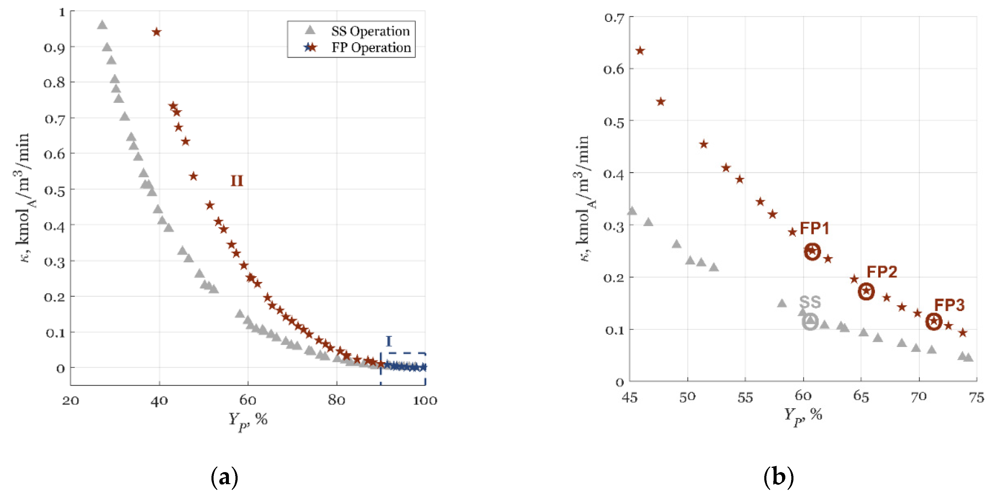
• Zone I (blue stars) was in the region of very low $\kappa$ and high $Y_P$, i.e., $\kappa$ ≈ 0 and $Y_P$ > 90%. In Figure 4a, Zone I is shown with a dashed rectangle. Both SS and FP operations showed the same trend of achieving the highest product yields $Y_P$, at the lowest CSTR volumetric capacities, $\kappa$ (Figure 4a). This was expected as the highest $Y_P$ could be achieved with negligible flow rates and in the smallest reactors, i.e., with the highest residence time (Figure 4a). Zone I showed that as $Y_P$ increases, the influence of PI through input modulation, or system nonlinearity enhancement, potential decreased when compared to the benefits of a higher reactor residence time. The result was complete reactant conversion for the SS and FP operations but with minimal production potential (low $\kappa$). Zone I was of no interest in this research because it lied in the region of negligible $\kappa$ and did not enhance the process significantly if the FP operation was utilized.
• In Zone II (red stars, $Y_P$ < 90%, Figure 4a), the FP operation showed PI potential while outperforming the optimal SS operation. Since Zone II was of interest for the dynamic enhancement of the CSTR process, it is also shown, in part, in Figure 4b. The same Pareto front was displayed on a different scale in Figure 4b with chosen cases for analysis: the SS case and the three FP cases of FP1, FP2, and FP3 (denoted with small circles in Figure 4b). For the chosen cases, optimal Pareto results can be seen in

  Table 3. Optimal product yield (BI1), reactor volumetric capacity (BI2/CI), and the corresponding optimized values for Example 1 (CSTR) for points SS, FP1, FP2, and FP3 in Figure 4b.

  Variable	SS	FP1	FP2	FP3
  $Y_P$, %	60.61	60.79	65.45	71.29
  $\kappa$, kmol/m3/min	0.12	0.25	0.17	0.12
  $F_s$, m3/min	0.18	0.28	0.14	0.16
  $C_{Ai,s}$, kmol/m3	19.04	19.95	19.91	19.87
  $V$, m3	29.07	32.11	22.86	39.25
  $A_1$, /		0.95	0.94	0.971
  $A_2$, /		0.97	0.97	0.964
  $\omega$, rad/s (Hz)		0.52 (8.3 × 10−2)	0.53 (8.5 × 10−2)	0.56 (8.9 × 10−2)
  $\phi$, rad		6.08	5.86	6.12

  .

As visible from Figure 3 and Table 3, the FP operation gave significantly higher $Y_P$ and $\kappa$ when compared to the optimal SS operation. The optimal operating parameters were rapidly determined thanks to the cNFR-supplied DC function files. In Appendix A, a detailed analysis of the MOO can be found. In the next example, the cNFR–MOO methodology is used to find an optimal FP operation for enhancing electrochemical oxygen reduction reaction, which is of industrial relevance.

3.2. Example 2: Electrochemical Oxygen Reduction Reaction Process (ECR)

3.2.1. Problem Formulation

The oxygen reduction reaction (ORR) is utilized in fuel cells, batteries, and some electrolysis processes. It is also of strong industrial relevance in processes that involve chlorine production [55]. The kinetics of the ORR were previously studied using the cNFR method by Kandaswamy et al. [55]. The first- and second-order symmetrical FRFs were verified for 0.1 M NaOH solution [55]. Živković et al. explained in detail how the FRFs were derived using the cNFR method [36]. In a subsequent study, the cNFR method was used to evaluate electrochemical process improvement if FP operation is utilized [56].

The ORR is taking place on the surface of a silver rotating disc electrode, with the assumed single-step mechanism [55]:

$$O_2+e^{-} \stackrel{ k_{app} }{\to } products$$

(18)

In total, six equations describe a single-step mechanism shown in Equation (18):

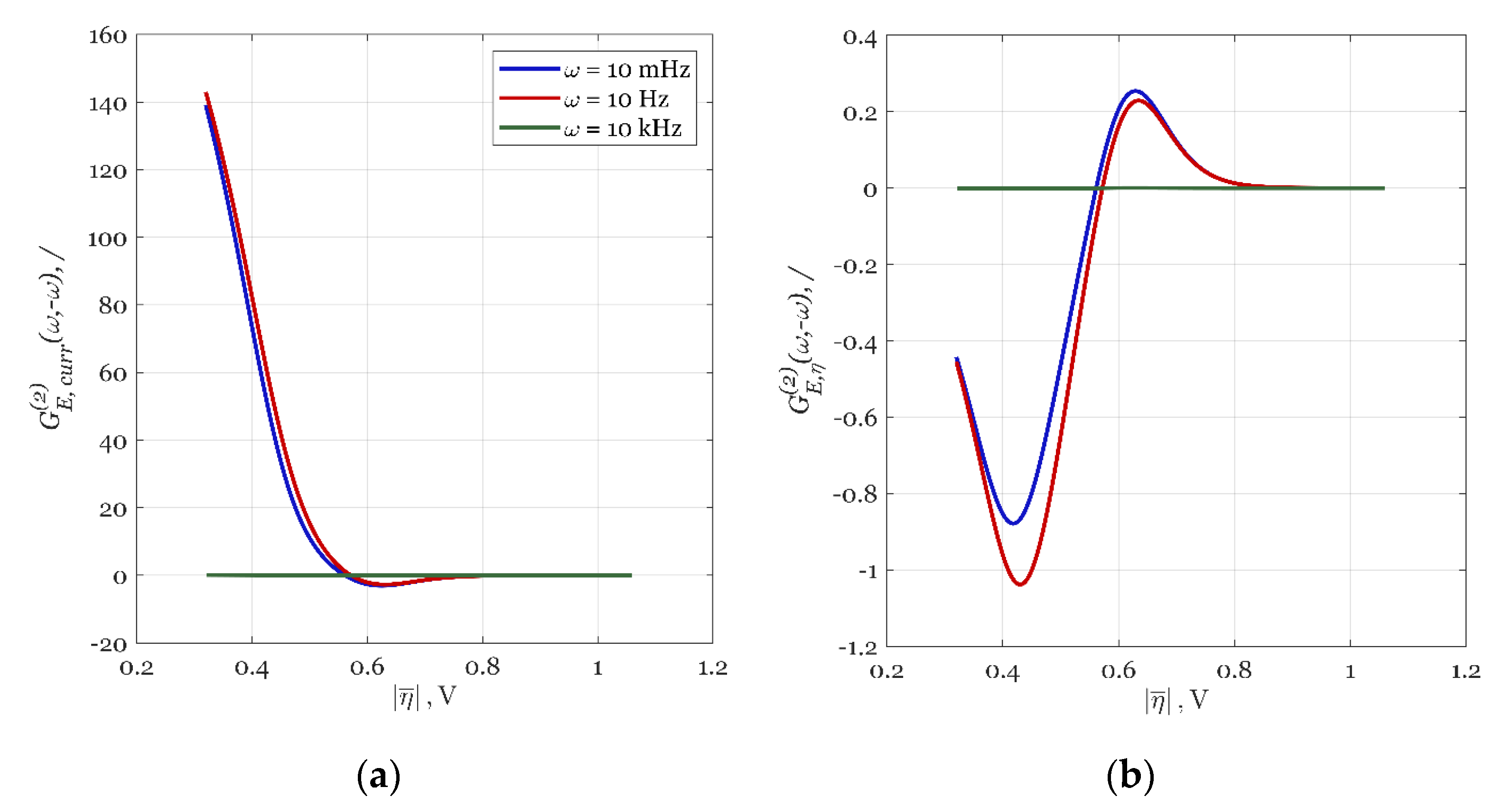
• The electrical charge balance:

  $$c_{dl}·\frac{d\eta \left(t\right)}{dt}=curr\left(t\right)+F·4·r\left(t\right)$$

  (19)

  where $c_{dl}$ is the double-layer capacitance, $\eta$ the electrode overpotential, $F$ the Faraday’s constant, $r$ the ORR reaction rate expression, and $curr$ the current density, which is the main output of interest.
• The potential balance:

  $$\eta \left(t\right)=E\left(t\right)-E^{\theta }-R_{\mathsf{\Omega }}·curr\left(t\right)$$

  (20)

  where $E$ is the electrode potential (which is a possible modulated input), $E^{\theta }$ is the standard electrode potential, and $R_{\mathsf{\Omega }}$ is the ohmic resistance.
• The reaction rate of the ORR:

  $$r\left(t\right)=k_{app}\left(t\right)·\frac{c_1\left(t\right)}{1+\frac{k_{app}\left(t\right)}{D/\left(\delta \left(t\right)/2\right)}}$$

  (21)

  where $k_{app}$ is the apparent rate constant of the ORR according to the equation:

  $$k_{app}\left(t\right)=k_{e1}·e^{-\frac{\alpha ·F}{R·T}·\eta \left(t\right)}$$

  (22)

  In Equation (22), $k_{e1}$ is the ORR kinetic constant, $\alpha$ is the transfer coefficient, $R$ is the universal gas constant, and $T$ is the reaction temperature, which is assumed to be constant.
• The intermediary oxygen concentration derived from the discretized mass balance Equation [55]:

  $$\frac{d{c}_1\left(t\right)}{dt}=\frac{D}{\delta {\left(t\right)}^2/2}·\left(c_{bulk}-c_1\left(t\right)\right)-\frac{D}{\delta {\left(t\right)}^2/2}·\frac{c_1\left(t\right)·k_{app}\left(t\right)}{D/\delta \left(t\right)+k_{app}\left(t\right)}$$

  (23)
• The electrode boundary layer thickness:

  $$\delta \left(t\right)=1.61·D^{\frac{1}{3}}·{\nu }^{\frac{1}{6}}·{\omega }_r{\left(t\right)}^{-\frac{1}{2}}$$

  (24)

  where ${\omega }_r$ is the electrode rotation rate, $D$ is the oxygen diffusivity in the boundary layer, and $\nu$ is the kinematic viscosity of the NaOH solution.

In the additional investigation, the second-order asymmetrical FRF and the corresponding DC component of the current density, $curr$ (when electrode potential, $E$, is periodically modulated), were experimentally verified by Živković et al. [56]. In the same research, the verified DC component was used to show that there can be significant ORR process improvement when $E$ is periodically modulated input, $x$, around its SS value, $E_s$ (according to equation in Figure 1) [56]:

$$E\left(t\right)=E_s·\left[1+A·\cos \left(\omega ·t\right)\right]$$

(25)

Here, the evaluation of the ORR FP operation was extended further by conducting rigorous cNFR–MOO.

3.2.2. Objective Functions, and Constraints Formulation

In a preliminary evaluation, the FP ORR operation was considered to be superior to the SS operation if the absolute mean value of the current density, $\left|\overline{curr}\right|$, was higher and the absolute mean value of the overpotential, $\left|\overline{\eta }\right|$, was lower [56]. Therefore, CI as $\left|\overline{\eta }\right|$, and BI as $\left|\overline{curr}\right|$ were seen to be two objective functions. These objective functions could be evaluated based on the corresponding asymmetrical second-order FRFs using the following equations [56]:

$$\min \left(CI\right)\mathrm{where}CI=\left|\overline{\eta }\right|=\left|{\eta }_s\right|·\left(1+D{C}_{E,\eta }\right)\approx \left|{\eta }_s\right|·\left[1+2·{\left(\frac{A}{2}\right)}^2·G_{E,\eta }^{\left(2\right)}\left(\omega ,-\omega \right)\right]$$

(26)

$$\max \left(BI\right)\mathrm{where}BI=\left|\overline{curr}\right|=\left|cur{r}_s\right|·\left(1+D{C}_{E,curr}\right)\approx \left|cur{r}_s\right|·\left[1+2·{\left(\frac{A}{2}\right)}^2·G_{E,curr}^{\left(2\right)}\left(\omega ,-\omega \right)\right]$$

(27)

In Equations (26) and (27), $G_{E,\eta }^{\left(2\right)}\left(\omega ,-\omega \right)$ and $G_{E,curr}^{\left(2\right)}\left(\omega ,-\omega \right)$ are the asymmetrical second-order FRFs for the periodically modulated potential $E$ (input variable), and $\eta$ and $curr$ are outputs of interest, respectively. The cNFR software gives the user MATLAB function files with the derived FRFs and the respective DC components in an algebraic, vector form. Thus, $\left|\overline{\eta }\right|$ and $\left|\overline{curr}\right|$ can be computed in an easy and fast manner. It should be noted that FRF $G_{E,curr}^{\left(2\right)}\left(\omega ,-\omega \right)$ was experimentally verified in a study by Živković et al. when higher current densities were achieved by using forced periodic operation [56].

One constraint for both the SS and FP operations is that the system must be stable. Therefore, the roots of the characteristic equation obtained by the cNFR equation have to be negative. The characteristic equation was derived in the same manner as for the previous example, and, due to its numerous and long equation terms, is not shown here. The MOO of the FP operation also has two additional constraints that satisfy the following inequality:

$$0.1<E_s·\left(1+A\right)<1$$

(28)

Equation (28) was introduced to ensure that at any time the potential at the electrode surface could not be higher than 1 V or lower than 0.1 V because, at those conditions, no ORR can physically occur.

3.2.3. Optimization Variables and Criteria Formulation

The optimization variables for both SS and FP operations are given in

Table 4. Pareto optimization variables for Example 2: ECR and its corresponding lower and upper bounds with scaling values (in brackets).

Variable	SS Operation		FP Operation
	Lower Bound	Upper Bound	Lower Bound	Upper Bound
$E_s$, V	0.1	1	0.1	1
${\omega }_r$, rpm	0.16 (×2500)	1 (×2500)	0.16 (×2500)	1 (×2500)
$A$, /			0	1
$\omega$, rad/s			10−3 (×2π)	103 (×2π)

. Two electrode operating variables were optimized in both operations: the electrode surface SS potential, $E_s$, and electrode rotation rate, ${\omega }_r$. $E_s$ cannot be lower than 0.1 or higher than 1 V, thus satisfying the inequality interval constraint (Equation (28)). The minimum possible ${\omega }_r$ was set to 400 rpm, and the maximum was set to 2500 rpm, well-within the technical limitations of the rotating device described by Kandaswamy et al. [55]. ${\omega }_r$ was scaled to be optimized between 0.16 and 1, and its real value was calculated by multiplying with the maximal allowed value of 2500 rpm, as shown in brackets in Table 4.

The FP operation has two additional, dynamic optimization variables: the amplitude of FP modulation $A$, and the frequency of modulation, $\omega$. $A$ was optimized between 0 and 1, while frequency was optimized between 10⁻³ and 10³ Hz, with its exponent as the optimization variable. The variable was further multiplied by 2π to obtain the radial frequency, $\omega$, in rad/s (Table 4).

The MOOs of the SS and FP operations were performed in MATLAB 2019b by using the same algorithm (NSGA-II). The criteria for NSGA-II, which are listed in

Table 5. Pareto optimization criteria for Example 2: ECR.

NSGA-II Criterion	Name	Value
Number of variables	Nvars	2 (SS), 4 (FP)
Population size	Pop	500
Max. number of generations	Gen	50,000
Pareto tolerance	FunctionTolerance	1 × 10−4
Parallel computing	UseParallel	true

, were the same as in Example 1 (Table 2), except that the number of optimized variables was now different (two for SS operation and four for FP operation) and parallel computing was used because of more constraint evaluations.

After conducting MOO on the same device as in Example 1, the total MOO time for the SS operation was 118 s and 324 s for the FP operation. The dynamic optimization took less than four minutes longer than the SS optimization.

3.2.4. Results and Discussion

The results of the MOOs for the SS and FP operations are shown in Figure 4. The SS operation (gray triangles in Figure 4a) gave an increased BI at a higher CI, as expected. The FP operation (colored stars in Figure 4a) showed a similar trend with a sudden discontinuity for the CI between approximately 0.5 and 0.65 V, i.e., at a BI of approximately 61 A/m².

Three distinctive PI zones, marked with different colored stars and surrounded with dashed rectangles and Roman numerals in Figure 4a, could be identified by analyzing the Pareto front:

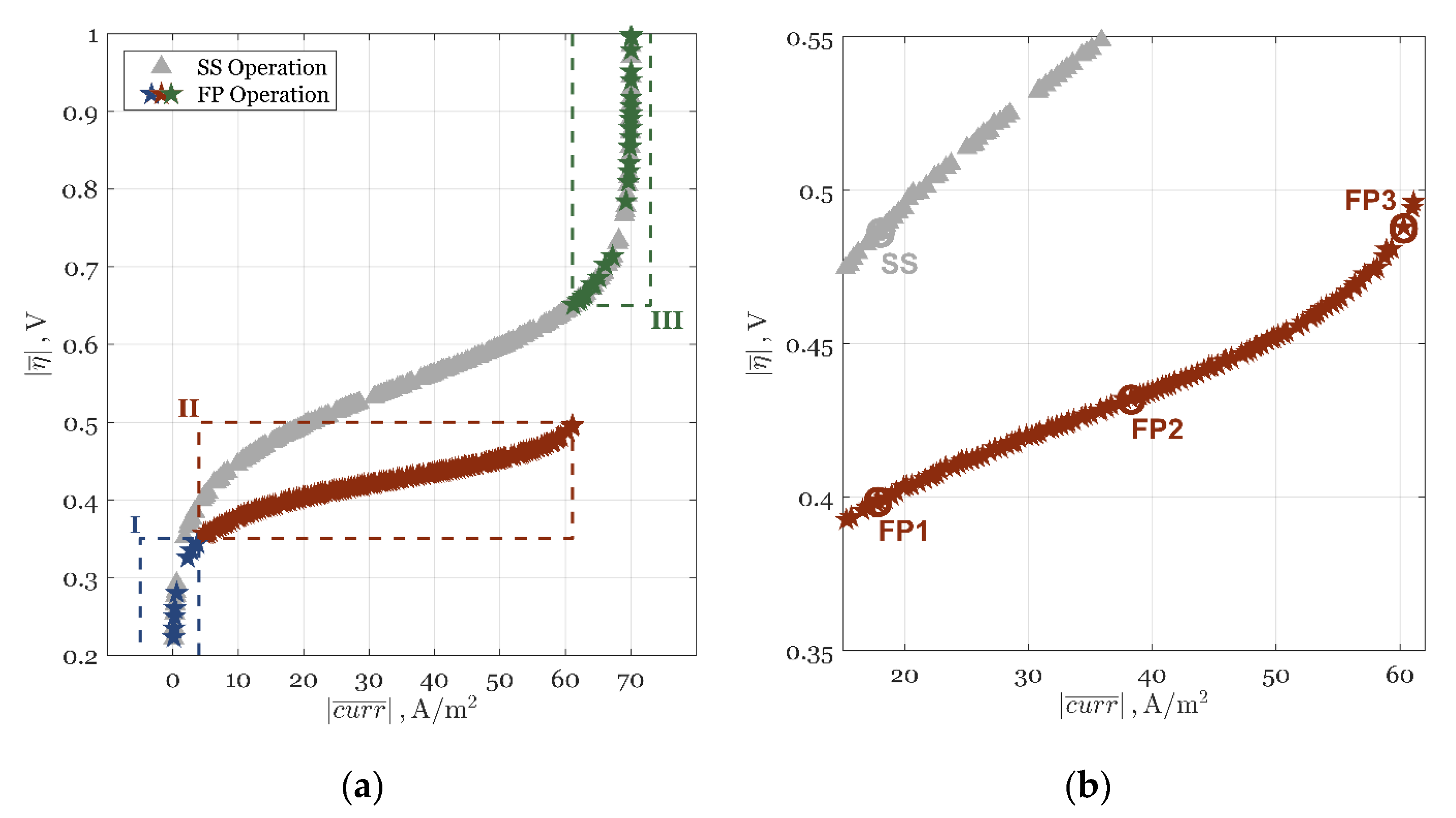
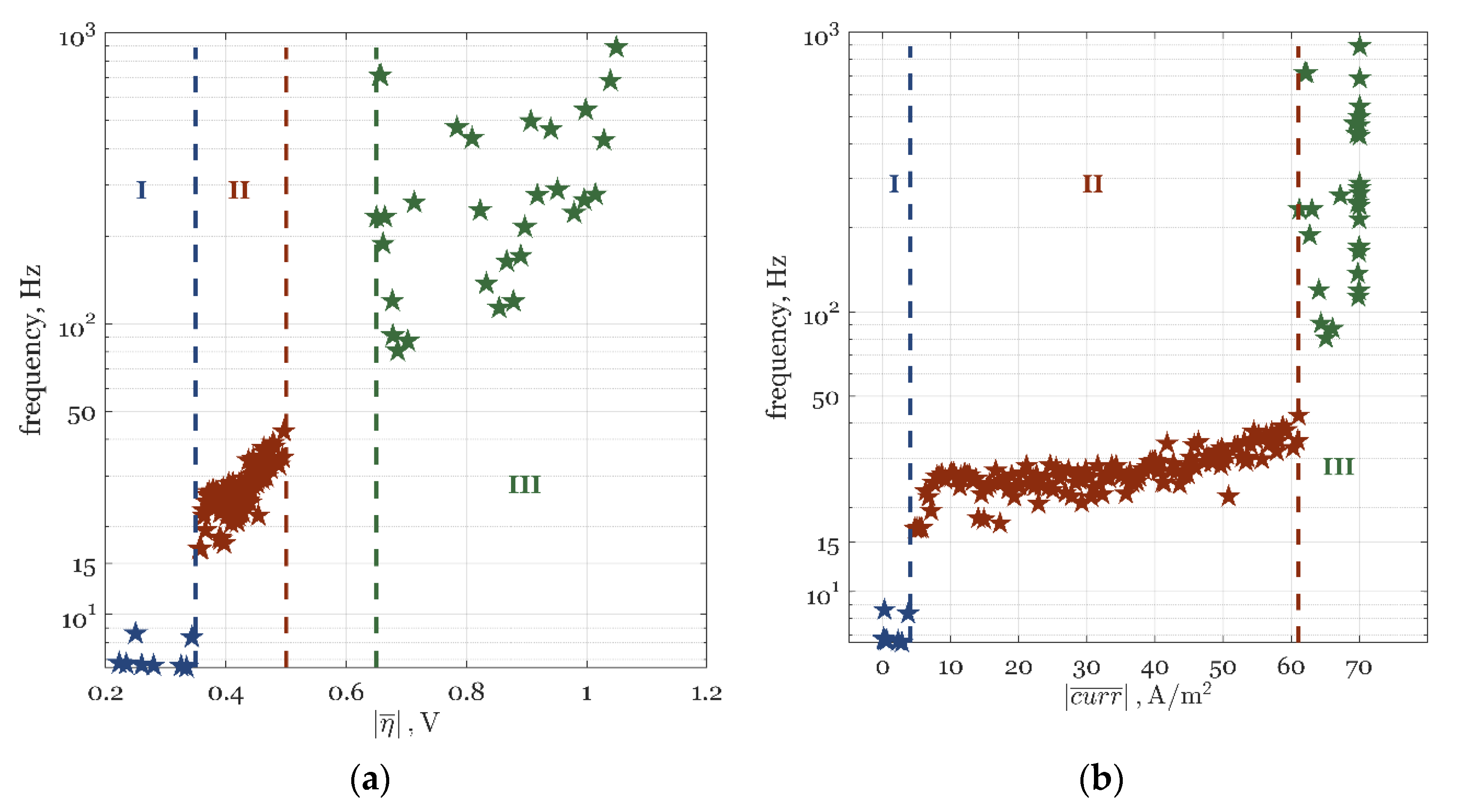
• Zone I (blue stars) was in the region of very low CI and BI, i.e., $\left|\overline{\eta }\right|$ < 0.35 V and $\left|\overline{curr}\right|$ < 4 A/m². In Zone I, both operations gave similar BI and CI and produced almost no current density. This zone was marked by the dominant kinetic regime and negligible ORR in the system.
• In Zone II (red stars), for 0.35 < $\left|\overline{\eta }\right|$ < 0.50 V and 4 < $\left|\overline{curr}\right|$ < 61 A/m², or until the discontinuity, the FP operation showed a strong PI potential and outperformed the SS operation as CI increased. This zone was of the highest interest in the dynamic enhancement of the ORR process and is also shown, in part, in Figure 4b.
• Zone III (green stars), which was in the range of high CI and BI, i.e., $\left|\overline{\eta }\right|$ > 0.65 V and $\left|\overline{curr}\right|$ > 61 A/m², showed no ORR enhancement as both SS and FP operations gave the same BI and CI. In this zone, incremental improvements in BI were very expensive as they could only be achieved at exponential increases in CI.

In

Table 6. Optimal current density (BI), overpotential (CI), and corresponding operational values for Example 2: ECR and Cases: SS, FP1, FP2, and FP3.

Variable	SS	FP1	FP2	FP3
$\left|\overline{curr}\right|$, A/m2	18.04	17.85	38.29	60.30
$\left|\overline{\eta }\right|$, V	0.487	0.399	0.432	0.488
$E_s$, V	0.717	0.805	0.751	0.674
${\omega }_r$, rpm	2483	2447	2496	2478
$A$, /		0.24	0.33	0.48
$\omega$, rad/s (Hz)		156 (24.9)	171 (27.3)	205 (32.7)

, optimal Pareto results for selected cases marked with circles in Figure 4b, along with the optimized operational values, are given. As can be seen both in Figure 4 and Table 6, the optimal FP operation outperformed the optimal SS operation in Zone II, both in BI and CI values. It should be noted that if MOO was not used but SOO with a combined CI and BI (in form BI/CI) was, the optimal solution would be in Zone III, thus resulting in no improvement with FP operation. By using MOO, the user can see all possible PI enhancement zones and identify operating FP conditions for which a 334% higher current density was achieved when compared to the SS case. A more detailed analysis of the Figure 4 and Table 6 results can be found in Appendix B.

The discontinuity line that occurred at $\left|\overline{curr}\right|$ ≈ 61 A/m², and 0.5 V < $\left|\overline{\eta }\right|$ < 0.65 V, was void of any optimal FP solutions (Figure 4a). This can be explained by the sudden change of sign of the respective FRF functions (Equations (26) and (27)). A more detailed analysis of the discontinuity and Zones I, II, and III can be found in Appendix C.

4. Conclusions

In this paper, we introduced a completely new approach to optimizing the forced periodic operations of processes that are classically operated in a steady-state regime. This was also the first time that the simultaneous optimization of both forced periodic and its corresponding operational steady-state point was performed for a chemical process in the frequency domain. The main contribution of this approach was based on combining multi-objective optimization techniques with the Nonlinear Frequency Response (NFR) method, which enables direct estimation of time-average values of the outputs of periodically operated processes. Thanks to the NFR method, the objective functions could be defined as algebraic expressions. These expressions depend on the steady-state point around which the system is perturbed, on one hand, and the forcing parameters of the input perturbations on the other. Recently, the NFR method was upgraded to the computer-aided Nonlinear Frequency Response (cNFR) method using a software tool for the automatic derivation of the frequency response functions (FRFs), which are crucial for applying the NFR method. The main advantages of the cNRF-based multi-objective optimization of periodic processes can be summarized as the following:

• The objective functions are defined in the form of algebraic expressions defining the time-average behavior of the periodic process, so there is no need for numerical solutions of the nonlinear dynamic model equations. Consequently, the computing times for the optimization of the periodic and the steady-state operations are of the same order of magnitude.
• Due to the automatic derivation of the FRFs using the cNRF software, defining and evaluating the objective functions of interest are fast and easy tasks. Periodic operations with one or two modulated inputs can be essentially treated in the same way.
• The new approach performs the optimization of the steady-state point and the forcing parameters in one step. In this way, in some cases, it is possible to find a periodic operation around a sub-optimal steady state that would be superior, not only to the steady-state operation but also to any periodic operation around the previously established optimal steady state.

The methodology for cNFR-assisted cost–benefit indicator multi-objective optimization was clearly defined and illustrated in two different cases: an isothermal continual stirred tank reactor (CSTR) with a simple reaction mechanism and two simultaneously modulated inputs—the reactant concentration and flow rate of the feed stream—and a process with electrochemical oxygen reduction reaction (ECR), with the modulation of only one input—the electrode potential. As shown in both CSTR and ECR examples, forced periodic operation can greatly intensify the process under the right operating conditions. When two inputs were modulated, the determination of the optimal phase angle, which was possible due to the cNFR-generated function files, was of the utmost importance. The product yield, the primary CSTR benefit indicator, was doubled under the FP operation when compared to the optimal SS operation with the same volumetric reactor capacity. Similarly, in the previously experimentally verified ECR example, the PI of the optimized FP operation led to a current density 3.34 times higher than in the optimized SS operation. The usefulness of the cNFR as a new PSE tool did not end there, as it enabled the detailed analysis of the obtained Pareto fronts through easy and quick simulations of the key FRFs. With the cNFR method, it was possible to identify all PI zones and then focus on optimal solutions with the highest potential for process improvement. In both examples, the speed of the multi-objective optimizations was remarkable (the dynamic optimizations were finished in several minutes), even at tightened tolerances and increased genetic algorithm populations.

As shown, the methodology for cNFR-based multi-objective optimization, presented in this work, can be a powerful PSE tool that could bring a new impulse to the promotion and implementation of forced periodic operations in the chemical industry.

References

- Douglas, J.M.; Rippin, D.W.T. Unsteady state process operation. Chem. Eng. Sci. 1966, 21, 305–315. [Google Scholar] [CrossRef]
- Douglas, J.M. Periodic reactor operation. Ind. Eng. Chem. Process. Des. Dev. 1967, 6, 43–48. [Google Scholar] [CrossRef]
- Horn, F.J.M.; Lin, R.C. Periodic processes: A variational approach. Ind. Eng. Chem. Process Des. Dev. 1967, 6, 21–30. [Google Scholar] [CrossRef]
- Bailey, J.E.; Horn, F.J.M. Improvement of the performance of a fixed-bed catalytic reactor by relaxed steady state operation. AIChE J. 1971, 17, 550–553. [Google Scholar] [CrossRef]
- Stankiewicz, A.; Kuczynski, M. An industrial view on the dynamic operation of chemical converters. Chem. Eng. Process. Process Intensif. 1995, 34, 367–377. [Google Scholar] [CrossRef]
- Tian, Y.; Demirel, S.E.; Hasan, M.M.F.; Pistikopoulos, E.N. An overview of process systems engineering approaches for process intensification: State of the art. Chem. Eng. Process. 2018, 133, 160–210. [Google Scholar] [CrossRef]
- Skiborowski, M. Process synthesis and design methods for process intensification. Curr. Opin. Chem. Eng. 2018, 22, 216–225. [Google Scholar] [CrossRef]
- Bui, M.; Gunawan, I.; Verheyen, V.; Feron, P.; Meuleman, E.; Adeloju, S. Dynamic modelling and optimisation of flexible operation in post-combustion co2 capture plants—A review. Comput. Chem. Eng. 2014, 61, 245–265. [Google Scholar] [CrossRef]
- Klatt, K.-U.; Hanisch, F.; Dünnebier, G.; Engell, S. Model-based optimization and control of chromatographic processes. Comput. Chem. Eng. 2000, 24, 1119–1126. [Google Scholar] [CrossRef]
- Logist, F.; Lauwers, J.; Trigaux, B.; Van Impe, J.F. Model based optimisation of a cyclic reactor for the production of hydrogen. In Computer Aided Chemical Engineering; Pistikopoulos, E.N., Georgiadis, M.C., Kokossis, A.C., Eds.; Elsevier: Amsterdam, The Netherlands, 2011; Volume 29, pp. 457–461. [Google Scholar]
- Nikačević, N.; Todić, B.; Mandić, M.; Petkovska, M.; Bukur, D.B. Optimization of forced periodic operations in milli-scale fixed bed reactor for fischer-tropsch synthesis. Catal. Today 2020, 343, 156–164. [Google Scholar] [CrossRef]
- Sildir, H.; Arkun, Y.; Canan, U.; Celebi, S.; Karani, U.; Er, I. Dynamic modeling and optimization of an industrial fluid catalytic cracker. J. Process Control 2015, 31, 30–44. [Google Scholar] [CrossRef]
- Toumi, A.; Engell, S.; Diehl, M.; Bock, H.G.; Schlöder, J. Efficient optimization of simulated moving bed processes. Chem. Eng. Process. Process Intensif. 2007, 46, 1067–1084. [Google Scholar] [CrossRef]
- Živković, L.A.; Nikačević, N.M. A method for reactor synthesis based on process intensification principles and optimization of superstructure consisting of phenomenological modules. Chem. Eng. Res. Des. 2016, 113, 189–205. [Google Scholar] [CrossRef]
- Özgülşen, F.; Adomaitis, R.A.; Çinar, A. A numerical method for determining optimal parameter values in forced periodic operation. Chem. Eng. Sci. 1992, 47, 605–613. [Google Scholar] [CrossRef]
- Bausa, J.; Tsatsaronis, G. Reducing the energy demand of continuous distillation processes by optimal controlled forced periodic operation. Comput. Chem. Eng. 2001, 25, 359–370. [Google Scholar] [CrossRef]
- Cruse, A.; Marquardt, W.; Allgor, R.J.; Kussi, J. Integrated conceptual design of stirred tank reactors by periodic dynamic optimization. Comput. Chem. Eng. 2000, 24, 975–981. [Google Scholar] [CrossRef]
- Vetukuri, S.R.R.; Biegler, L.T.; Walther, A. An inexact trust-region algorithm for the optimization of periodic adsorption processes. Ind. Eng. Chem. Res. 2010, 49, 12004–12013. [Google Scholar] [CrossRef]
- Tsay, C.; Pattison, R.C.; Baldea, M. A pseudo-transient optimization framework for periodic processes: Pressure swing adsorption and simulated moving bed chromatography. AIChE J. 2018, 64, 2982–2996. [Google Scholar] [CrossRef]
- Gao, X.; Chen, B.; He, X.; Qiu, T.; Li, J.; Wang, C.; Zhang, L. Multi-objective optimization for the periodic operation of the naphtha pyrolysis process using a new parallel hybrid algorithm combining NSGA-II with SQP. Comput. Chem. Eng. 2008, 32, 2801–2811. [Google Scholar] [CrossRef]
- Hakanen, J.; Kawajiri, Y.; Miettinen, K.; Biegler, L.T. Interactive multi-objective optimization for simulated moving bed processes. Control Cybern. 2007, 36, 283–302. [Google Scholar]
- De la Torre, V.; Walther, A.; Biegler, L.T. Optimization of periodic adsorption processes with a novel problem formulation and nonlinear programming algorithm. In Proceedings of the AD 2004–Fourth International Workshop on Automatic Differentiation, Argonne National Laboratory, Lemont, IL, USA, 19–23 July 2004. [Google Scholar]
- Rangaiah, G.P.; Feng, Z.; Hoadley, A.F. Multi-objective optimization applications in chemical process engineering: Tutorial and review. Processes 2020, 8, 508. [Google Scholar] [CrossRef]
- Ghiasi, H.; Pasini, D.; Lessard, L. A non-dominated sorting hybrid algorithm for multi-objective optimization of engineering problems. Eng. Optim. 2011, 43, 39–59. [Google Scholar] [CrossRef]
- Živković, L.A.; Pohar, A.; Likozar, B.; Nikačević, N.M. Reactor conceptual design by optimization for hydrogen production through intensified sorption- and membrane-enhanced water-gas shift reaction. Chem. Eng. Sci. 2020, 211, 115174. [Google Scholar] [CrossRef]
- Abu-Reesh, I.M. Single- and multi-objective optimization of a dual-chamber microbial fuel cell operating in continuous-flow mode at steady state. Processes 2020, 8, 839. [Google Scholar] [CrossRef]
- Wang, M.; Li, Y.; Yuan, J.; Meng, F.; Appiah, D.; Chen, J. Comprehensive improvement of mixed-flow pump impeller based on multi-objective optimization. Processes 2020, 8, 905. [Google Scholar] [CrossRef]
- De, R.; Bhartiya, S.; Shastri, Y. Multi-objective optimization of integrated biodiesel production and separation system. Fuel 2019, 243, 519–532. [Google Scholar] [CrossRef]
- Mitsos, A.; Asprion, N.; Floudas, C.A.; Bortz, M.; Baldea, M.; Bonvin, D.; Caspari, A.; Schäfer, P. Challenges in process optimization for new feedstocks and energy sources. Comput. Chem. Eng. 2018, 113, 209–221. [Google Scholar] [CrossRef]
- Schilling, J.; Tillmanns, D.; Lampe, M.; Hopp, M.; Gross, J.; Bardow, A. From molecules to dollars: Integrating molecular design into thermo-economic process design using consistent thermodynamic modeling. Mol. Syst. Des. Eng. 2017, 2, 301–320. [Google Scholar] [CrossRef]
- De, R.; Bhartiya, S.; Shastri, Y. Multi-objective optimization of a batch transesterification reactor considering reactor and methanol separation unit together. In Computer Aided Chemical Engineering; Espuña, A., Graells, M., Puigjaner, L., Eds.; Elsevier: Amsterdam, The Netherlands, 2017; Volume 40, pp. 2203–2208. [Google Scholar]
- Mamaghani, A.H.; Najafi, B.; Shirazi, A.; Rinaldi, F. Exergetic, economic, and environmental evaluations and multi-objective optimization of a combined molten carbonate fuel cell-gas turbine system. Appl. Therm. Eng. 2015, 77, 1–11. [Google Scholar] [CrossRef]
- Hreiz, R.; Roche, N.; Benyahia, B.; Latifi, M.A. Multi-objective optimal control of small-size wastewater treatment plants. Chem. Eng. Res. Des. 2015, 102, 345–353. [Google Scholar] [CrossRef]
- Baldea, M.; Edgar, T.F. Dynamic process intensification. Curr. Opin. Chem. Eng. 2018, 22, 48–53. [Google Scholar] [CrossRef]
- Petkovska, M.; Seidel-Morgenstern, A. Evaluation of periodic processes. In Periodic Operation of Reactors; Silveston, P.L., Hudgins, R.R., Eds.; Butterworth-Heinemann: Oxford, UK, 2013; pp. 387–413. [Google Scholar]
- Živković, L.A.; Vidaković-Koch, T.; Petkovska, M. Computer-aided nonlinear frequency response method for investigating the dynamics of chemical engineering systems. Processes 2020, 8, 1354. [Google Scholar]
- Petkovska, M.; Do, D.D. Nonlinear frequency response of adsorption systems: Isothermal batch and continuous flow adsorbers. Chem. Eng. Sci. 1998, 53, 3081–3097. [Google Scholar] [CrossRef]
- Petkovska, M.; Do, D.D. Use of higher-order frequency response functions for identification of nonlinear adsorption kinetics: Single mechanisms under isothermal conditions. Nonlinear Dyn. 2000, 21, 353–376. [Google Scholar] [CrossRef]
- Marković, A.; Seidel-Morgenstern, A.; Petkovska, M. Evaluation of the potential of periodically operated reactors based on the second order frequency response function. Chem. Eng. Res. Des. 2008, 86, 682–691. [Google Scholar] [CrossRef]
- Nikolic Paunic, D.; Petkovska, M. Evaluation of periodic processes with two modulated inputs based on nonlinear frequency response analysis. Case study: Cstr with modulation of the inlet concentration and flow-rate. Chem. Eng. Sci. 2013, 104, 208–219. [Google Scholar] [CrossRef]
- Nikolić, D.; Seidel-Morgenstern, A.; Petkovska, M. Periodic operation with modulation of inlet concentration and flow rate. Part I: Nonisothermal continuous stirred-tank reactor. Chem. Eng. Technol. 2016, 39, 2020–2028. [Google Scholar] [CrossRef]
- Currie, R.; Nikolic, D.; Petkovska, M.; Simakov, D.S.A. CO2 conversion enhancement in a periodically operated sabatier reactor: Nonlinear frequency response analysis and simulation-based study. Isr. J. Chem. 2018, 58, 762–775. [Google Scholar] [CrossRef]
- Nikolić, D.; Felischak, M.; Seidel-Morgenstern, A.; Petkovska, M. Periodic operation with modulation of inlet concentration and flow rate part II: Adiabatic continuous stirred-tank reactor. Chem. Eng. Technol. 2016, 39, 2126–2134. [Google Scholar] [CrossRef]
- Nikolić, D.; Petkovska, M. Evaluation of performance of periodically operated reactors for single input modulations of general waveforms. Chem. Ing. Tech. 2016, 88, 1715–1722. [Google Scholar] [CrossRef]
- Nikolić, D.; Seidel-Morgenstern, A.; Petkovska, M. Nonlinear frequency response analysis of forced periodic operation of non-isothermal cstr with simultaneous modulation of inlet concentration and inlet temperature. Chem. Eng. Sci. 2015, 137, 40–58. [Google Scholar] [CrossRef][Green Version]
- Nikolić, D.; Seidel-Morgenstern, A.; Petkovska, M. Nonlinear frequency response analysis of forced periodic operation of non-isothermal cstr using single input modulations. Part I: Modulation of inlet concentration or flow-rate. Chem. Eng. Sci. 2014, 117, 71–84. [Google Scholar] [CrossRef][Green Version]
- Nikolić, D.; Seidel-Morgenstern, A.; Petkovska, M. Nonlinear frequency response analysis of forced periodic operation of non-isothermal cstr using single input modulations. Part II: Modulation of inlet temperature or temperature of the cooling/heating fluid. Chem. Eng. Sci. 2014, 117, 31–44. [Google Scholar] [CrossRef]
- Nikolic Paunic, D. Forced Periodically Operated Chemical Reactors—Evaluation and Analysis by The Nonlinear Frequency Response Method; Faculty of Technology and Metalurgy, University of Belgrade: Belgrade, Serbia, 2016; under review. [Google Scholar]
- Petkovska, M.; Nikolić, D.; Seidel-Morgenstern, A. Nonlinear frequency response method for evaluating forced periodic operations of chemical reactors. Isr. J. Chem. 2018, 58, 663–681. [Google Scholar] [CrossRef]
- Nikolić, D.; Seidel-Morgenstern, A.; Petkovska, M. Nonlinear frequency response analysis of forced periodic operations with simultaneous modulation of two general waveform inputs with applications on adiabatic cstr with square-wave modulations. Chem. Eng. Sci. 2020, 226, 115842. [Google Scholar] [CrossRef]
- Bensmann, B.; Petkovska, M.; Vidaković-Koch, T.; Hanke-Rauschenbach, R.; Sundmacher, K. Nonlinear frequency response of electrochemical methanol oxidation kinetics: A theoretical analysis. J. Electrochem. Soc. 2010, 157, B1279−B1289. [Google Scholar] [CrossRef]
- Petkovska, M.; Marković, A. Fast estimation of quasi-steady states of cyclic nonlinear processes based on higher-order frequency response functions. Case study: Cyclic operation of an adsorption column. Ind. Eng. Chem. Res. 2006, 45, 266–291. [Google Scholar] [CrossRef]
- Petkovska, M.; Nikolić, D.; Marković, A.; Seidel-Morgenstern, A. Fast evaluation of periodic operation of a heterogeneous reactor based on nonlinear frequency response analysis. Chem. Eng. Sci. 2010, 65, 3632–3637. [Google Scholar] [CrossRef]
- Vidaković-Koch, T.R.; Panić, V.V.; Andrić, M.; Petkovska, M.; Sundmacher, K. Nonlinear frequency response analysis of the ferrocyanide oxidation kinetics. Part I. A theoretical analysis. J. Phys. Chem. C 2011, 115, 17341–17351. [Google Scholar] [CrossRef]
- Kandaswamy, S.; Sorrentino, A.; Borate, S.; Živković, L.A.; Petkovska, M.; Vidaković-Koch, T. Oxygen reduction reaction on silver electrodes under strong alkaline conditions. Electrochim. Acta 2019, 320, 134517. [Google Scholar] [CrossRef]
- Živković, L.A.; Kandaswamy, S.; Petkovska, M.; Vidaković-Koch, T. Evaluation of electrochemical process improvement using computer-aided nonlinear frequency response method: Oxygen reduction reaction in alkaline media. Front. Chem. 2020, in press. [Google Scholar]