Connecting Risk and Resilience for a Power System Using the Portland Hills Fault Case Study

Abstract

Active seismic faults in the Pacific Northwest area have encouraged electric utilities in the region to deeply contemplate and proactively intervene to support grid resilience. To further this effort this research introduces Monte Carlo (MC)-based power system modeling as a means to inform the Performance Based Earthquake Engineering method and simulates 100,000 sample earthquakes of a 6.8 magnitude (M6.8) Portland Hills Fault (PHF) scenario in the Portland General Electric (PGE) service territory as a proof of concept. This paper also proposes the resilience metric Seismic Load Recovery Factor (SLRF) to quantify the recovery of a downed power system and thus can be used to quantify earthquake economic risk. Using MC results, the SLRF was evaluated to be 19.7 h and the expected economic consequence cost of a M6.8 PHF event was found to be $180 million with an annualized risk of $90,000 given the event’s 1 in 2000 year probability of occurrence. The MC results also identified the eight most consequential substations in the PGE system—i.e., those that contributed to maximum load loss. This paper concludes that retrofitting these substations reduced the expected consequence cost of a M6.8 PHF event to $117 million.

1. Introduction

Portland, Oregon, and Vancouver, Washington, metropolitan area is in a seismically active region of the Pacific Northwest USA. The Portland Hills Fault (PHF) forms the southwest boundary of the Portland Basin with the adjacent Portland Hill and is the most significant local seismic source [1]. For this study we consider a representative earthquake event that can occur from the PHF. An earthquake magnitude of 6.8 (M6.8) is selected as it is an upper bound earthquake that can be generated from the PHF and this provides a representative earthquake scenario for a risk assessment study for planning, emergency preparedness/response, and loss estimation for infrastructures located within the city of Portland, Oregon. Power system resilience has several definitions, but are consistent in three main ideas: (1) preparation, (2) absorption and (3) recovery, from any high-impact low-probability event such as hurricanes, ice-storms, and earthquakes. To quantify resilience better a conceptual resilience curve is described in the paper [2]. Using this resilience curve many different resilience metrics have been proposed, such as Vulnerability Index (VI), Degradation Index (DI), Restoration Efficiency Index (REI) and Microgrid Resilience Index (MRI) [3], and the $\mathsf{\Phi }$, $\mathsf{\Lambda }$, $\mathcal{E}$, $\mathsf{\Pi }$ system [4,5].

The study presented in this paper aims to estimate the potential risk of a Portland Hills Fault event, and also identify the best locations for investment for risk reduction. The methodology for this study is designed around the intent of providing an economic basis for making decisions about seismic upgrades. Portland General Electric (PGE) being the local electrical utility is interested in knowing which upgrades will produce cost effective reductions in seismic risk based on logical progression of the following questions. If there is an earthquake, how violently will the ground shake at a given location? Given the shaking, what is the chance various pieces of equipment will break/fail? If the equipment fails, what will be the cost to customers and what might be done to reduce that cost? To answer these questions, the complete methodology needs to be divided into 4 parts and each of these parts and its corresponding background literature is discussed in detail in the following sections. The 4 parts are:

(1)

Ground shaking analysis,

(2)

Structural analysis,

(3)

Load-flow Monte Carlo analysis and

(4)

Economic consequence analysis.

The necessity of the first 3 steps and use of the Performance Based Earthquake Engineering (PBEE) method is discussed in the [6,7,8]. Although this study focuses on the Portland Hills Fault case study using the Western Electrical Coordinating Council (WECC) model as the power grid model, it also intends to propose the overall framework used for this case study as a larger framework to connect risk and resilience of any power system. All additional background for the proposed framework can be found in [9].

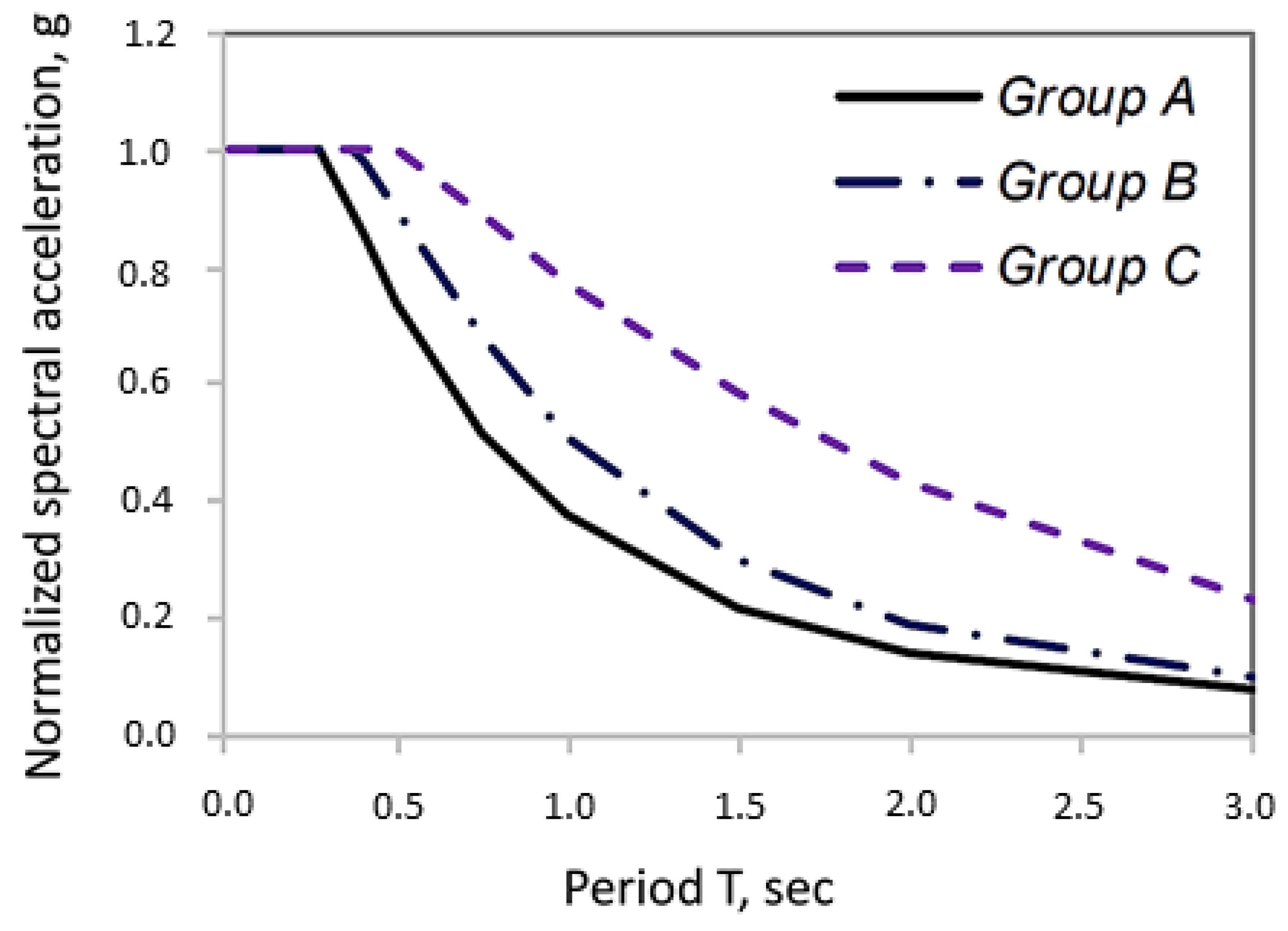
2. Ground Shaking Analysis

2.1. Methodology for Ground Shaking Analysis

The objective of this analysis is to obtain information on all the substations that would be affected by the M6.8 PHF earthquake scenario and gather ground shaking data (i.e., Peak Ground Acceleration (PGA) values) for these substation. To that end we perform a Deterministic Seismic Hazard Analysis (DSHA) to estimate the ground shaking intensities during a M6.8 PHF event. The main steps in a deterministic ground motion evaluation for a M6.8 PHF fault include: (1) Determining the seismic source characterization of the PHF and the appropriate (shortest) distance from the PHF to each of the substation. (2) Selecting ground motion prediction models for calculation of the ground shaking intensities. (3) Calculating the ground shaking intensities at all substation sites.

We reviewed pertinent, readily available reports, scientific literature, maps and data regarding the PHF to assess the fault location and parameters [1,10,11,12]. Based on these results we developed potential rupture scenarios that could generate a M6.8 PHF earthquake. The United States Geological Survey’s (USGS’s) seismic source model for the Pacific Northwest region uses the most current source parameters for PHF to develop the national seismic hazard maps [13,14]. These maps, available online [15], are used to obtain the fault parameters used in the seismic hazard analysis for this research. For our study, a best estimate fault rupture length of 30 km was estimated for a M6.8 PHF earthquake based on empirical equations relating earthquake Moment Magnitude to surface rupture length and rupture area. Figure 1 shows the fault trace with 30 km portions highlighted at the north (orange) and south (pink) end of the PHF. Three rupture scenarios at the north end, center and the south end were considered but only the rupture at the north end of the fault trace is used to further calculate the Peak Ground Acceleration (PGA) at the site of affected substations. The green spots in Figure 1 are the substations that are affected by a M6.8 PHF north end rupture scenario.

Deterministic design spectra are computed using ground motion prediction models that estimate ground motion as a function of earthquake rupture distance to the site, earthquake magnitude, and site conditions. To estimate ground motion associated with earthquakes that occur in tectonically active regions, such as the surrounding region that hosts the PHF, we reviewed several state-of-the art ground motion prediction models and selected four models based on their technical soundness. These selected models [16,17,18,19] are all from the suite of Pacific Earthquake Engineering Research (PEER) center sponsored Next-Generation Attenuation—West 2 Project [20]. These set of alternative models are given equal weights in the DSHA. The ground motion prediction models provide estimates of spectral accelerations in the period (T) of 0 to 10 seconds. Further the spectral acceleration for the period T = 0 seconds and for the north end rupture is used to calculate the PGA values at the substation sites as shown is Figure 2.

2.2. Assumptions Made during Ground Shaking Analysis

There are two types of uncertainties associated with ground motion calculation: (1) aleatory; and (2) epistemic. Aleatory is the uncertainty from the earthquake being a random process and is associated with the variability in the ground motions. The epistemic is the uncertainty that originates from alternative modeling approaches, datasets and interpretations. Epistemic uncertainties are accommodated through alternative prediction models, and are attributable to the lack of knowledge or data that contributes to the uncertainty in estimating model parameters. Due to the limited site-specific subsurface soil information and the empirical approach used to develop the earthquake and soil parameters, the calculated ground shaking intensities include very large uncertainties that should be refined if more precise values are desired for design purposes. Soil liquefaction hazard was not explicitly evaluated due to the lack of site-specific soil information, and therefore its impacts are excluded from the study.

2.3. Results of Ground Shaking Analysis

Through this process it was determined that there is a total of 71 substations in PGE’s service area that are at risk from the M6.8 PHF north end rupture. And based on their latitude and longitude the PGA values are calculated using the spectral acceleration for period T = 0 s. These PGA values are in the range of 0.10 to 0.55 g as can be observed the Figure 2. For perspective, the gravitational acceleration of planet earth is 1 g. We also calculated the probability of occurrence of all different scenarios that can cause the M6.8 PHF earthquake event and after summing all the probabilities for all probable scenarios the final probability of an event of this magnitude was calculated to be a 1 in 2000 years.

3. Structural Analysis

3.1. Methodology for Structural Analysis

After calculating the PGAs at all the 71 affected substation locations, we calculate the structural fragility of all the relevant assets at these locations. As we are interested in studying the impacts of the M6.8 PHF earthquake event on the power transmission system, we limit the scope to the asset/structure combinations that are rated for only transmission level voltages. To that end we select 3 voltage levels for this study: 57 kV, 115 kV and 230 kV. We further limit the scope of this study to three main types of substation assets: (1) Circuit Breakers (CB’s), (2) Transformers (TX’s) and (3) Disconnect Switches (DSW’s). We evaluate the structural fragility of 3 main types of assets (CB’s, TX’s and DSW’s), because these asset types are expected to contribute the most to seismic risk and also going ahead we intend to run power flow simulations on the Node-Breaker (NB) model of the power system. In the NB model the instrument transformers and control enclosures are not modeled. Further transmission lines are not included in the scope because the study is limited to substations assets. To that end all other equipment is assumed to be always operational. This finalizes the scope of this study to 508 total assets, which consists of 259 CB’s, 237 DSW’s and 12 TX’s, that are at risk from the M6.8 PHF north end rupture.

For ground shaking analysis we developed unique response spectra for each substation potentially impacted by the M6.8 PHF scenario earthquake. In order to reduce the number of structural analysis cases, these response spectra are arranged into 3 groups, A, B and C with similar normalized spectral shapes as described in Figure 3. These spectral shapes are primarily influenced by the soil profile beneath the substation. The response spectra, shown in Figure 3, characterize the earthquake acceleration that is expected to be experienced by structures with different fundamental periods of vibration. These response spectra are used in combination with the structural analysis models to calculate the seismic demands on asset/structure combinations that is further used in development of seismic fragility curves. Fragility data on substation assets and structures can be generated using actual earthquake damage data, experimental data, or analytical approaches. For this project, we used an analytical approach to develop fragility curves for representative PGE asset/structure combinations. The seismic response of an individual asset/structure combination is determined by either a response spectrum analysis or a static analysis. We use the information about typically observed failure mechanisms in substation assets to identify the most critically stressed points within an individual asset/structure combination and monitor the stresses at these points during analysis. The uncertainties in seismic response and capacity are quantified to determine the probabilities of failure corresponding to various levels of earthquake ground acceleration. The fragility analysis methodology implemented for this project is consistent with the methodology used in [21].

The analysis conducted to characterize the seismic fragility of a particular asset/structure combination requires data about the asset’s weight, geometry, bushing/insulator dimensions and wall thickness, structural support member sizes, foundation and anchorage details, etc. To that end we use several sources to compile the data necessary for fragility analysis. These sources encompass substation drawings, PGE’s asset database, manufacturer’s product catalogs, manufacturer inquiries for specific assets, substation site visits and discussions with PGE’s substation engineering staff. We developed an analytical model for each asset/structure combination using the structural analysis computer program SAP2000. These models include both the support structure and the electrical assets. Modal response spectrum analysis is used to determine the expected seismic demands at critical points of the support structure and the electrical asset. We consider earthquake ground motions acting in two orthogonal directions for this analysis. The expected seismic demand on a particular element is determined using the square root of the sum of squares (SRSS) method for a combination of analysis results in the two orthogonal directions.

The structural capacity of concrete anchors is calculated based on ACI 318-14, building code requirements for structural concrete [22] and the structural capacity of welds, bolts, and other steel elements is calculated based on AISC 360-10, specifications for structural steel buildings [23]. However, strength reduction factors are not used. We used, if available, the manufacturer’s rated maximum terminal pad loading or insulator cantilever strength to define the structural capacity of the electrical asset. Otherwise, the calculated strength of porcelain insulators and bushings is consistent with the maximum stress methodology used in [21]. Both seismic demand and structural capacity are assumed to follow a log-normal distribution. Seismic fragility curves are developed for several different potential failure mechanisms such as rocking, anchorage failure, bushing/insulator failure, etc. The fragility curve that predicts the largest probability of failure at a given value of PGA represents the anticipated primary failure mechanism and defines the fragility for that PGA. In most cases, it is observed that one failure mechanism controlled the asset fragility over the entire range of PGAs investigated (0.0–2.0 g). In a few cases, the controlling failure mechanism is observed to change above a certain value of PGA and the envelope of the controlling fragility curves is then used to define the fragility of the asset/structure combination.

3.2. Assumptions Made during Structural Analysis

For this study we developed limited fragility curves for representative electrical assets and their support structure combinations. It is assumed that the fragility curves developed for the representative combinations apply to the whole family of assets. When developing the seismic fragility curves for this study we do not include the potential impacts of the interaction of adjacent assets that are connected through rigid bus or flexible conductors without adequate slack. Asset failures caused due to soil liquefaction are also ignored.

3.3. Results of Structural Analysis

Using the methodology described for the structural analysis, the seismic fragility curves are developed for 3 different types of electrical assets, for 3 different transmission level voltages and for 3 different groups of assets as shown in Figure 4. A combination of the electrical assets and their support structures is considered for the development of these curves. The developed seismic fragility curves characterize the probability of failure (PoF) of a given asset for varying levels of earthquake-induced peak ground acceleration. So, for example a 115 KV DSW from group A, has a 20% PoF at 0.5 g PGA.

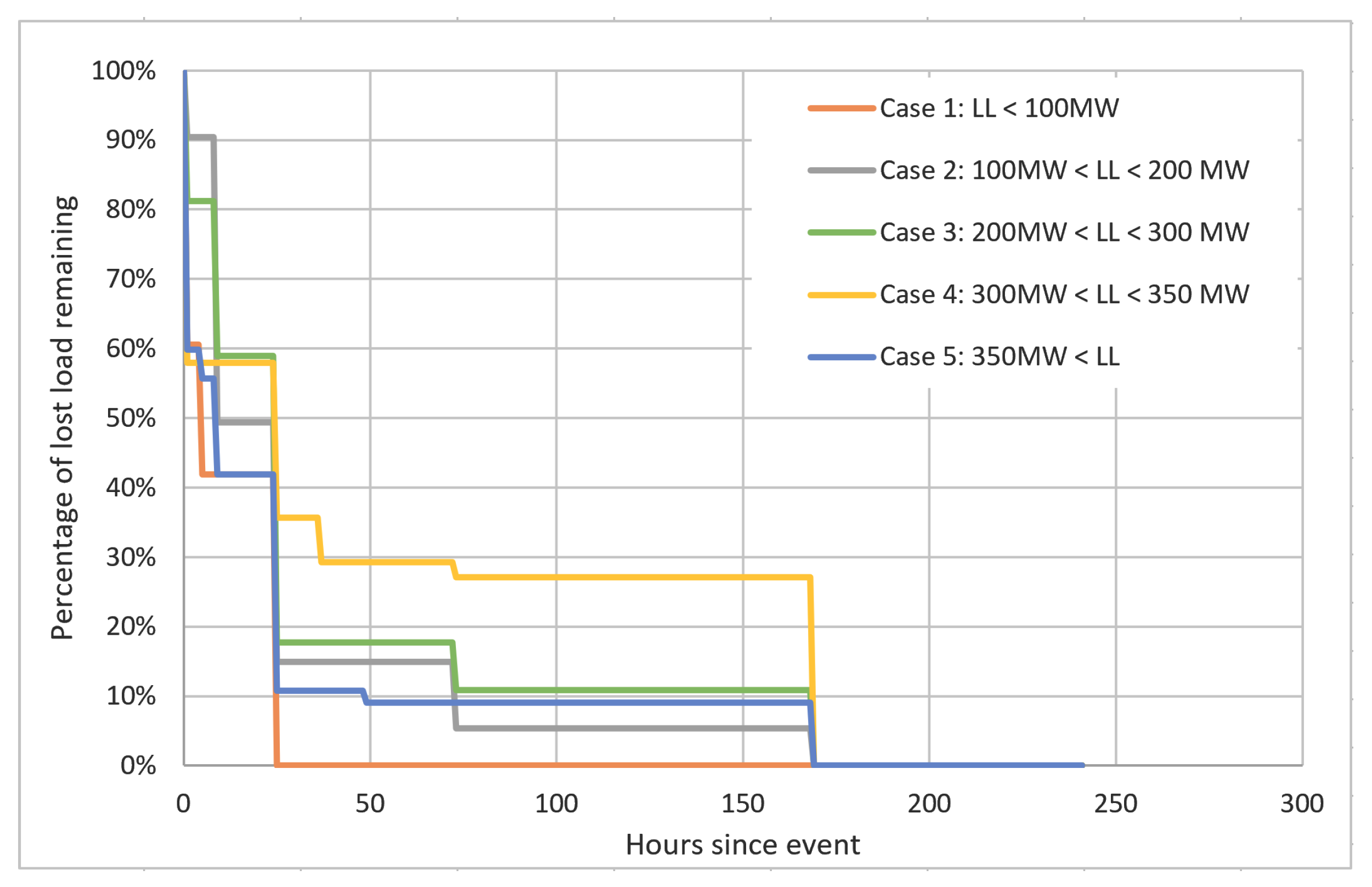
4. Load-Flow Monte Carlo Analysis

4.1. Methodology for Load-Flow Monte Carlo Analysis

From the ground shaking analysis we narrowed down the 71 substations, 508 electrical assets across 3 different voltage levels and from the structural analysis we developed their individual probability of failure for the M6.8 PHF north end rupture earthquake event. To apply an individual component’s fragility and simulate the earthquake event on a power transmission system, we use the NB (node-breaker) configuration of the Western Electrical Coordinating Council (WECC) model which includes 10 year ahead planning case information of PGE’s network. The case-file for this model is developed by Peak Reliability. Peak Reliability is listed on the North American Electric Reliability Corporation’s (NERC) compliance registry performing the reliability coordinator (RC) function for the Pacific Northwest region.

The case-file for the NB configuration of the WECC model is built for PGE by Peak Reliability using Powerworld and is proprietary. Powerworld is the load-flow solving software used for this study and is also the software used by PGE. The flowchart shown in Figure 5. describes the architecture used for the load-flow Monte Carlo analysis (LFMCA). We use the data generated from the ground shaking analysis to know the PGA values at the location of each asset. Using these PGA values, we calculate the PoF for every asset that is affected in PGE’s service area using the fragility curves. Then for one Monte Carlo simulation (i.e., One sample of the M6.8 PHF earthquake scenario), we generate one random number per asset and compare it with the PoF of the assets. This gives us a list of all the assets lost for that particular Monte Carlo simulation. Using this information, we remove the lost assets from the power system and connect the system that survived the earthquake event. This is followed by running a steady state load-flow analysis on the system that survived using the NB configuration of the WECC model. At the end of each Monte Carlo simulation and steady state load-flow analysis, we calculate and log the values of load/demand served by all load buses. For this study we simulated 100,000 Monte Carlo simulations. The Powerworld case-file (“.pwb” format) used for carrying out steady state load-flows simulates the peak load for PGE’s service area, which is 3156.97 MW.

We use the Python 3.6 to develop the Monte Carlo model because of the capability of Python to interface with the load-flow solver Powerworld, using SimAuto as the communication server. To reduce the overall simulation time for all 100,000 simulations, a parallel processing method is used. All simulations are divided into 8 processes of 12,500 simulations each. The division of simulations into several processes was also limited by the computational power available. At the end, the simulation time was clocked at 1.2 s/simulation making the complete simulation time to be approximately 33.5 h. For a proof of concept this simulation time was considered acceptable.

4.2. Assumptions for Load-Flow Monte Carlo Analysis

For LFMCA, we run a steady state load-flow for each Monte Carlo simulation. For this analysis, it is assumed that in the case of an island formation, because of the lost assets, all load on the island is considered lost. This assumption is based on the location of the PHF. There are no generation facilities in the area and thus it is safe to assume the demand on the islands cannot be supplied. The generators in the power system are assumed to always be operational because there are none located in the vicinity that would be directly affected by a PHF earthquake event.

It is also assumed that all the transmission lines in the power system will always be operational. This is because transmission towers are designed for high wind and ice loading, which in most cases exceeds earthquake stresses [24]. Towers are susceptible to damage from landslides and liquefaction, but those effects are not considered in this study.

4.3. Results of Load-Flow Monte Carlo Analysis

From Monte Carlo simulations we obtain the total load served at the end of each simulation. We subtract that from the peak load of the system to get the load loss (or size of the initial outage $L_{out,init}$) for each simulation. We then calculate the number of simulations with load loss in steps of 20 MW. This data is then plotted as the probability distribution of load loss as shown in Figure 6. Approximately 3% of all Monte Carlo simulations led to a non-converging load-flow scenario. We solved all non-converging simulations using two main techniques: (1) By changing the initial conditions used for the steady state load-flow analysis we solved approximately 65% these simulations and (2) By correcting asset models not in PGE’s service territory. We use the final load loss probability distribution data as the starting point for the economic consequence analysis.

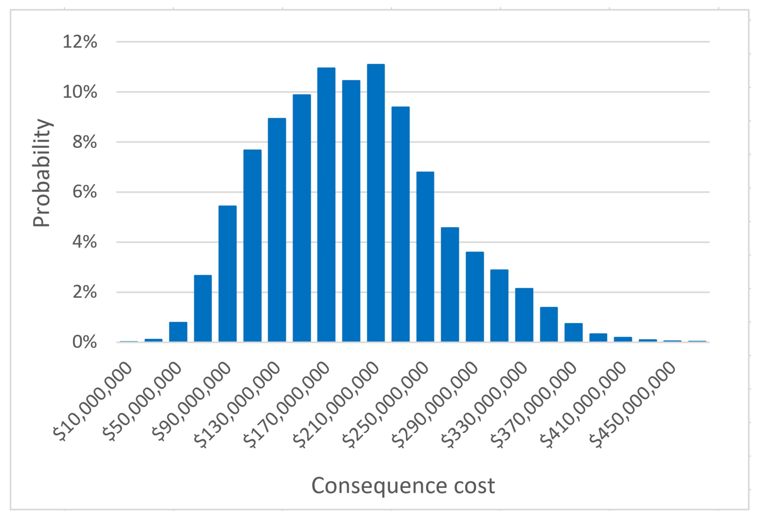
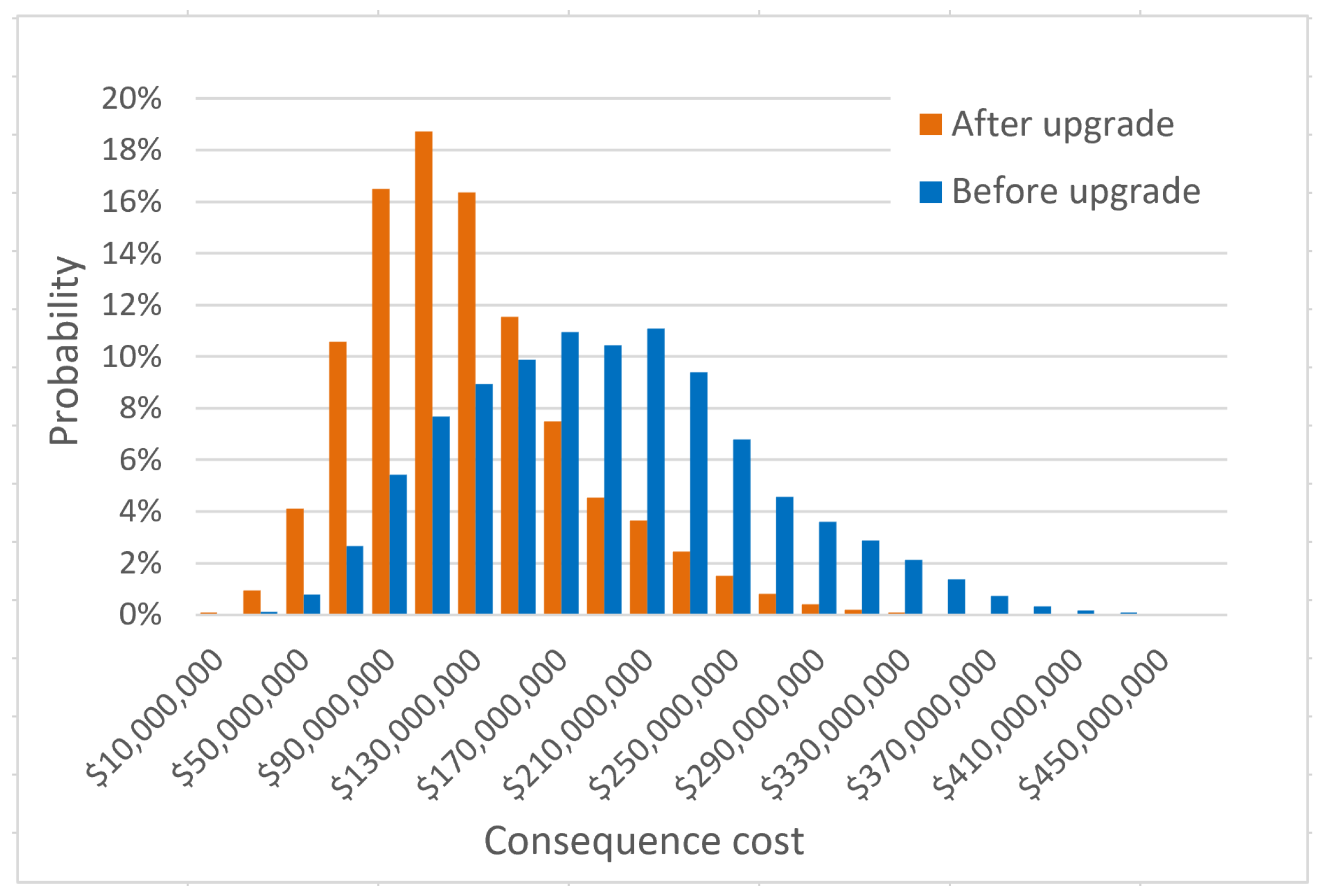
5. Economic Consequence Analysis

5.1. Methodology for Economic Consequence Analysis

The economic consequence analysis is carried out in two main steps: (1) Evaluating the economic consequence of the earthquake event with respect to an electrical utility and (2) Evaluating a targeted upgrade/retrofitting scenario and checking its impacts on the economic consequences. First, to evaluate the economic consequence we recognized that there are two factors affecting the consequence: (1) Consequence cost depending on the size of the initial outage (event cost) and, (2) Consequence cost depending on the duration of the outage (duration cost).

From the results of the LFMCA we directly get the size of initial outages which we converted into a dollar value using the standard prices used by PGE. This is calculated based on the $/kW by customer type (residential, commercial and industrial) and the fraction of total load per customer type. However, the more consequential part of the cost is the outage duration cost. To calculate the outage duration cost we developed a restoration model to calculate the duration of any outage. To develop the restoration model, we first select several earthquake cases from the LFMCA. The load loss (LL) in these cases ranges from 30 MW to 380 MW. For each of these cases we develop a restoration strategy using four factors: (1) Loads restored immediately due to automatic switching, (2) Loads restored in hours due to manual switching and simple fixes, (3) Loads that would require days to restore due to the need for temporary construction and (4) Loads that would require a week or more to restore due to the need for new equipment or major reconstruction. The hours it would take to restore 100% of lost load for five different cases is shown in Figure 7.

Using the data points from these cases we plot the fitted decay curve of the percent of outage remaining as a function of time since the event, and is shown in Figure 8. The gray dots are the timing and percentage of load remaining when step-changes in lost load occurred in the five cases shown in Figure 7. For the final fit, each point is weighted inversely with time since the event, this forces a better fit to the near-term changes than the long-term ones. We believe this is realistic modeling of our confidence in the estimates. The load out ($L_{out}$) as a function of time (t) and the size of initial outage ($L_{out,init}$) can then be represented using (1).

$$L_{out}(t,L_{out,init})=L_{out,init}·e^{-(0.37+0.035·t)}$$

(1)

$$SLRF={\int }_0^{\infty }{e}^{-(0.37+0.035·t)}dt$$

(2)

Where the exponential term [$e^{-(0.37+0.035·t)}$] represents the decay curve in Figure 8. We propose that the area under the exponential decay curve shown in Figure 8 be used as a metric for evaluating seismic resilience of a power system. We define it as the Seismic Load Recovery Factor (SLRF). SLRF can be calculated using (2) and its unit is hours. For this study we calculated SLRF = 19.7 h. We use SLRF to calculate the duration cost by multiplying the initial outage size to SLRF. For example the outage duration cost of a case with initial outage size of 20 MW will be calculated based on 20 × 19.7 MWh of energy not served. In the end the final consequence is obtained by adding the cost based on initial outage size ($/kW) and the cost based on the outage duration/energy not served ($/kWh).

For the second part of the economic consequence analysis we analyze the impacts of targeted upgrade/retrofitting efforts on the economic consequence. For this we first develop a set of upgraded fragility curves which assumes that the primary cause of failure has been mitigated. Therefore, for example, if rocking is the primary phenomenon leading to failure for the 230 kV circuit breakers then we assume an intervention in which we retrofitted the asset and now the probability of failure is dominated by the secondary phenomenon like bushing fracture. A comparison between these upgraded fragility curves (after intervention) and the curves we initially developed (before intervention) are shown in Figure 9. Then we rerun the LFMCA followed by the economic consequence cost calculation for the after-upgrade scenario to validate the importance of specific upgrading/retrofitting efforts.

5.2. Assumptions for Economic Consequence Analysis

It is assumed that the total load lost is divided into 50% commercial, 10% industrial and 40% residential load fractions. This assumption is made based on PGE’s demand portfolio and the cost for the outages were calculated based on these fractions. For developing the restoration model we did not consider any future upgrades.

5.3. Results of Economic Consequence Analysis

By adding the consequence costs based on the initial outage size and the duration of the outage, using the SLRF value equal to 19.7 h, we calculate the final economic consequence for each sample. We do this for all 100,000 Monte Carlo samples. Figure 10 shows the probability mass distribution of the consequence cost developed for this study, which has a mean value of $180 million. We calculated in the ground shaking analysis that the probability of a M6.8 PHF earthquake event is 1 in 2000 years. This leads to $90,000 in annualized risk of this event. If we consider a constant 5% rate of interest, then the net present value (NPV) of the future risk is equal to $1.8 million for this earthquake event.

From Figure 11 we observe that the cumulative probability of the consequence cost greater than $300 million is approximately 6%. These are low probability but high-impact scenarios. This means that even though it is unlikely that this earthquake event will lead to large consequence, the consequence cost of the highly unlikely event is so high that it is important that steps be taken to mitigate this risk.

When developing the restoration strategies for cases with high load losses we observed that there are common assets that reappear frequently in the list of lost assets. We studied these further and narrowed down 8 most consequential substations out of the 71 scoped substations. We re-ran the LFMCA by implementing the upgraded fragility curves (Figure 9) to the assets at these particular 8 substations followed by the economic consequence analysis for the upgraded scenario. The comparison of the probability distribution of the economic consequences for the before and after upgrade scenarios is shown in Figure 12. It is observed that the probability of a consequence cost greater than $300 million is completely negated by only upgrading 8 out of 71 substations. We also observe that the expected consequence cost for the upgraded system is reduced to $117 million leading to a reduced annual risk of $58,000. The NPV of future risk has also fallen from $1.8 million to $1.2 million, for a total avoided risk benefit of $600,000.

In Figure 12 it is also observed that the 99th percentile cost before upgrades is approximately $450,000,000, and the 99th percentile cost after upgrades is approximately $330,000,000. This suggests that the near-worst-case scenario of economic consequence before upgrades has been mitigated and the after-upgrade near-worst-case economic consequence is approximately $120,000,000 less. This avoidance of the extreme high-impact low-probability scenarios proves the effectiveness and the cost benefit of the suggested upgrades.

6. Conclusions

A novel and important contribution of this research is the development of a complete analytical framework which accepts quantitative input from geotechnical, structural, and electrical experts, leading to an economic evaluation of current seismic risk and the benefits of possible upgrades by studying the substation outages that lead to highest Value at risk (VaR) and conditional value at risk (CVaR). Traditional resilience metrics, which in many cases are calculated from the resilience curve, are often focused on measures of system performance and have an indirect connection to economic risk. The other main contribution of this paper is the proposed Seismic Load Recovery Factor (SLRF) as a metric for seismic resilience of a power transmission system, which has a direct connection to economic risk evaluation and helps the utility directly gauge grid’s ability to recover rapidly. We also demonstrate how SLRF is used to directly tie the impact of the earthquake scenario to the dollar value of the economic risk calculated. We found SLRF to be 19.7 h for this study using direct inputs from our utility partner, PGE.

The outage cost and seismic risk were quantified in “before upgrade” and “after-upgrade” scenarios, where it was assumed that the primary factor leading to asset failure was mitigated in only a selected 8 out of 71 substations. The selection of these substations was done based on the co-relation of substation outages or a combination of substation outages leading to the maximum economic consequence. This was done because an individual substation loss might not cause a large economic consequence but a combination of substations when lost might cause a large economic loss. So these combinations were recognized and upgrades were recommended for a total expected value of avoided risk benefit being $0.6 million.

The intent of this proof of concept study is to demonstrate that the methodology can feasibly be applied to evaluate actual spending options that will affect a range of earthquake scenarios. Furthermore, even though this study successfully proves that, it is important to note that this is a proof of concept study and the results presented in this paper does not represent or indicate the following: The impact, a PHF M6.8 earthquake or any another earthquake, may have on the PGE system; PGE’s disaster preparedness and ability to recover from an earthquake; Costs PGE may incur while recovering from an earthquake; and Lastly PGE’s future investment plans to enhance earthquake resiliency.

References

1. Wong, I.; Silva, W.; Bott, J.; Wright, D.; Thomas, P.; Gregor, N.; Li, S.; Mabey, M.; Sojourner, A.; Wang, Y. Earthquake Scenario and Probabilistic Ground Shaking Maps for the Portland, Oregon, Metropolitan Area. 2000. Available online: https://www.oregongeology.org/pubs/ims/ims-016/Text/Ims-16text.pdf (accessed on 22 September 2020).
2. Panteli, M.; Mancarella, P. The grid: Stronger bigger smarter: Presenting a conceptual framework of power system resilience. IEEE Power Energy Mag. 2015, 13, 58–66. [Google Scholar] [CrossRef]
3. Amirioun, M.; Aminifar, F.; Lesani, H.; Shahidehpour, M. Metrics and quantitative framework for assessing microgrid resilience against windstorms. Int. J. Electr. Power Energy Syst. 2019, 104, 716–723. [Google Scholar] [CrossRef]
4. Panteli, M.; Mancarella, P.; Trakas, D.; Kyriakides, E.; Hatziargyriou, N. Metrics and quantification of operational and infrastructure resilience in power systems. IEEE Trans. Power Syst. 2017, 32, 4732–4742. [Google Scholar] [CrossRef] [Green Version]
5. Panteli, M.; Trakas, D.N.; Mancarella, P.; Hatziargyriou, N. Power systems resilience assessment: Hardening and smart operational enhancement strategies. Proc. IEEE 2017, 105, 1202–1213. [Google Scholar] [CrossRef] [Green Version]
6. Chalishazar, V.; Fox, I.; Hagan, T.; Cotilla-Sanchez, E.; Jouanne, A.V.; Zhang, J.; Brekken, T.; Bass, R.B. Modelling power system buses using performance based earthquake engineering methods. In Proceedings of the 2017 IEEE Power & Energy Society General Meeting, Chicago, IL, USA, 16–20 July 2017; pp. 1–5. [Google Scholar]
7. Chalishazar, V.; Johnson, B.; Cotilla-Sanchez, E.; Brekken, T. Augmenting the traditional bus-branch model for seismic resilience analysis. In Proceedings of the 2018 IEEE Energy Conversion Congress and Exposition (ECCE), Portland, OR, USA, 23–27 September 2018; pp. 1133–1137. [Google Scholar]
8. Johnson, B.; Chalishazar, V.; Cotilla-Sanchez, E.; Brekken, T.K. A monte carlo methodology for earthquake impact analysis on the electrical grid. Electr. Power Syst. Res. 2020, 184, 106332. [Google Scholar] [CrossRef]
9. Chalishazar, V.H. Evaluating the Seismic Risk and Resilience of an Electrical Power System. Ph.D. Thesis, Oregon State University, Corvallis, OR, USA, 2019. [Google Scholar]
10. Yelin, T.S.; Patton, H.J. Seismotectonics of the portland, oregon, region. Bull. Seismol. Soc. Am. 1991, 81, 109–130. [Google Scholar]
11. Liberty, L.M.; Hemphill-Haley, M.A.; Madin, I.P. The portland hills fault: Uncovering a hidden fault in portland, oregon using high-resolution geophysical methods. Tectonophysics 2003, 368, 89–103. [Google Scholar] [CrossRef]
12. Wong, I.G.; Hemphill-Haley, M.A.; Liberty, L.M.; Madin, I.P. The portland hills fault: An earthquake generator or just another old fault. Or. Geol. 2001, 63, 39–50. [Google Scholar]
13. Petersen, M.D.; Zeng, Y.; Haller, K.M.; McCaffrey, R.; Hammond, W.C.; Bird, P.; Moschetti, M.; Shen, Z.-K.; Bormann, J.; Thatcher, W.R. Geodesy-And Geology-Based Slip-Rate Models for the Western United States (Excluding California) National Seismic Hazard Maps; U.S. Geological Survey: Reston, VA, USA, 2014. [Google Scholar]
14. Petersen, M.D.; Frankel, A.D.; Harmsen, S.C.; Mueller, C.S.; Haller, K.M.; Wheeler, R.L.; Wesson, R.L.; Zeng, Y.; Boyd, O.S.; Perkins, D.M. Documentation for the 2008 Update of the United States National Seismic Hazard Maps; Technic Report; Geological Survey (US): Reston, VA, USA, 2008. [Google Scholar]
15. National Seismic Hazard Maps. Available online: https://earthquake.usgs.gov/hazards/hazmaps/conterminous/index.php#2014 (accessed on 9 February 2019).
16. Abrahamson, N.A.; Silva, W.J.; Kamai, R. Summary of the ask14 ground motion relation for active crustal regions. Earthq. Spectra 2014, 30, 1025–1055. [Google Scholar] [CrossRef]
17. Boore, D.M.; Stewart, J.P.; Seyhan, E.; Atkinson, G.M. Nga-west2 equations for predicting pga, pgv, and 5% damped psa for shallow crustal earthquakes. Earthq. Spectra 2014, 30, 1057–1085. [Google Scholar] [CrossRef] [Green Version]
18. Campbell, K.W.; Bozorgnia, Y. Nga-west2 ground motion model for the average horizontal components of pga, pgv, and 5% damped linear acceleration response spectra. Earthq. Spectra 2014, 30, 1087–1115. [Google Scholar] [CrossRef]
19. Chiou, B.S.-J.; Youngs, R.R. Update of the chiou and youngs nga model for the average horizontal component of peak ground motion and response spectra. Earthq. Spectra 2014, 30, 1117–1153. [Google Scholar] [CrossRef]
20. Bozorgnia, Y.; Abrahamson, N.A.; Atik, L.A.; Ancheta, T.D.; Atkinson, G.M.; Baker, J.W.; Baltay, A.; Boore, D.M.; Campbell, K.W.; Chiou, B.S.-J. Nga-west2 research project. Earthq. Spectra 2014, 30, 973–987. [Google Scholar] [CrossRef] [Green Version]
21. Huo, J.-R.; Hwang, H.H. Seismic Fragility Analysis of Equipment and Structures in a Memphis Electric Substation; National Center for Earthquake Engineering Research: Buffalo, NY, USA, 1995. [Google Scholar]
22. ACI. Building Code Requirements for Reinforced Concrete (aci 318-14); ACI: Dhaka, Bangladesh, 2014. [Google Scholar]
23. AISC. Specification for Structural Steel Buildings (ansi/aisc 360-10); American Institute of Steel Construction: Chicago, IL, USA, 2010. [Google Scholar]
24. Park, H.-S.; Choi, B.H.; Kim, J.J.; Lee, T.-H. Seismic performance evaluation of high voltage transmission towers in south korea. KSCE J. Civ. Eng. 2016, 20, 2499–2505. [Google Scholar] [CrossRef]
Figure 1. Map of Portland Hills Fault (PHF) location with north, middle and south rupture scenarios.
Processes 08 01200 g001
Figure 2. Spectral acceleration for period T = 0 s for the Portland Hills Fault (M = 6.8) north end rupture scenario.
Processes 08 01200 g002
Figure 3. Normalized response spectra for 3 categories/groups of assets A, B and C.
Processes 08 01200 g003
Figure 4. Fragility curves for circuit breakers (blue), disconnect switch (black) and transformers (yellow) for 57 kV, 115 kV and 230 kV voltage levels and for all 3 groups of assets A, B and C.
Processes 08 01200 g004
Figure 5. Flow chart for the Monte Carlo model architecture.
Processes 08 01200 g005
Figure 6. Load loss probability distribution (Peak load = 3156.97 MW).
Processes 08 01200 g006
Figure 7. Outage duration for 5 cases with load loss (LL) ranging from 30 MW to 380 MW.
Processes 08 01200 g007
Figure 8. The exponential decay curve for the fraction of the outage remaining as a function of time.
Processes 08 01200 g008
Figure 9. Comparison of initial (before intervention) and after upgrade (after intervention) fragility curves for 8 different types of assets.
Processes 08 01200 g009
Figure 10. Probability distribution of the outage consequence cost.
Processes 08 01200 g010
Figure 11. Cumulative probability for the outage consequence cost.
Processes 08 01200 g011
Figure 12. Comparison of “before upgrade” (blue) and “after upgrade” (orange) probability distributions of the outage consequence cost.
Processes 08 01200 g012