Novel 3-D T-Shaped Passive Micromixer Design with Helicoidal Flows

Abstract

Laminar fluid flow and advection-dominant transport produce ineffective mixing conditions in micromixers. In these systems, a desirable fluid mixing over a short distance may be achieved using special geometries in which complex flow paths are generated. In this paper, a novel design, utilizing semi-circular ridges, is proposed to improve mixing in micro channels. Fluid flow and scalar transport are investigated employing Computational Fluid Dynamics (CFD) tool. Mixing dynamics are investigated in detail for alternative designs, injection, and diffusivity conditions. Results indicate that the convex alignment of semi-circular elements yields a specific, helicoidal-shaped fluid flow along the mixing channel which in turn enhances fluid mixing. In all cases examined, homogenous concentration distributions with mixing index values over 80% are obtained. When it is compared to the classical T-shaped micromixer, the novel design increases mixing index and mixing performance values by the factors of 8.7 and 3.3, respectively. It is also shown that different orientations of ridges adversely affect the mixing efficiency by disturbing the formation of helicoidal-shaped flow profile.

1. Introduction

During the past few decades, design of the micro-scale systems field has attracted researchers from various disciplines of science. This is essentially due to numerous advantages of size reduction and extensive applicability of these systems in diverse academic and industrial platforms. In general, microfluidic concept presents as an efficient, portable, safe, and low-cost [1,2,3,4,5] operating environment for various practices in the fields of chemistry [6,7], biology and biotechnology [8,9], medical [10,11], and environmental applications [8,9,12]. Micromixers are usually considered as one of the major components of microfluidic systems [10,13] which are commonly defined as micro total analysis systems (µTAS) or lab-on-a-chip (LOC) devices [6,14]. While serving as an integrated mixing element in miniaturized systems, micromixers can also be used as a stand-alone device [8]. The main role of these micro-scale units is to mix two or more fluids homogenously and rapidly over a short mixing channel. Micromixers are generally classified as active or passive depending on the mixing principles employed [8,9,15,16]. Active micromixers use external disturbance fields, such as magnetic, acoustic, thermal and electrical etc., [5] and perform well for short distances. However, extra energy and therefore component requirement create complexity in terms of integration of these units with other microchip elements [12,17]. Whereas, passive micromixers use the energy in the flow system in micro channels and present better integrability with microfluidic systems. The prominent benefits of passive micromixers have motivated several researchers to focus on improving the mixing performance and reduce mixing length in these units.

In passive micromixers, highly laminar fluid flow (e.g., Reynolds (Re) < 100 [11]) and low molecular diffusion constants (e.g., typically D = 10⁻⁹−10⁻¹¹ m²/s [18]) create a challenging mixing environment. This is mostly due to advection-dominant transport developed in micro channels (i.e., Peclet (Pe) >> 1). Although decreasing the flowrate promote diffusive mixing, obtaining an adequate mixing efficiency requires quite long channels which may exceed microchip dimensions [19]. Hence, developing special design topologies in passive micromixers is essential to improve mixing efficiency and reduce mixing length. This is usually achieved by generating secondary flows or transversal velocity components in micro channels by which interfacial area between fluid bodies increase. In the current passive micromixer literature, numerous micromixer designs are proposed to enhance mixing accordingly. These configurations mostly include simple channel modifications [20,21,22,23,24,25], obstructed channels [26,27,28,29,30,31], grooved geometries [32,33,34,35,36,37], and injection-based designs to manipulate flow in plain micro channels [38,39,40,41,42]. Due to smooth design architecture and fabrication process, simple 3-D geometries (e.g., Y-, and T-shaped), consisting of inlet and mixing channels, are broadly studied under various injection strategies and channel modifications. For example, Afzal and Kim [26] investigated a split-and-recombination (SAR) type micromixer for a Re range 10–70. The design proposed enhance mixing by generating secondary flows in sub-channels. More than 80% mixing efficiency is obtained at the exit of the micromixer (i.e., around 10 mm) in cases where Re is greater than 30. The range of pressure drops reported is around 3–10 kPa for corresponding Re numbers 30–70 in the best-case scenario tested. Alam et al. [27] studied the effects of obstructions in curved and straight channels for various flowrates (e.g., 0.1 ≤ Re ≤ 60). It was shown that compared to the plain curved channel, adding obstacles significantly increases mixing efficiency at low Re numbers tested. While hexagonal and circular mixing elements perform similarly, the effect of diamond obstacles is less than other two shapes until Re = 50 is reached. Employing the circular obstacles, authors obtained mixing efficiency values around 88% on the outlet plane (i.e., 5 mm axial distance) for Re = 0.1 and Re > 15 flow scenarios. Pressure drops are reported as 10 kPa and 23 kPa at Re = 60 for straight and curved channels respectively. Gidde and Pawar [13] surveyed a three-inlet passive micromixer with rectangular and elliptic baffles for Re numbers between 0.1 and 50. The micromixers examined activate vortex generation and provide over 85% mixing efficiency for Re ≥ 10. Pressure drops, obtained at Re = 50, are nearly 40 kPa and 30 kPa for rectangular- and elliptic-baffle configurations respectively. Chen et al. [36] performed a numerical and experimental study on a passive micromixer with crosswise ridges positioned in the mixing channel. It is shown that the generation of rotational flows along the mixing channel promotes fluid mixing. Mixing lengths, predicted to reach 90% efficiency, are reported as 4.86 cm and 3.65 cm for Re numbers 0.05 and 50 respectively. Wang et al. [32] attached cylindrical grooves on lateral walls of a rectangular duct. Results indicate that creation of transversal velocities inside the grooves considerably improve mixing efficiency in a distance less than 20 mm for a Re number range 1–100. Authors obtained the lowest pressure drop around 9.3 kPa for Re = 100 scenario.

Aside from the obstruction and grooved designs, several researchers focused on generating vortex or engulfment flows in plain micro channels. For instance, Ansari et al. [43] proposed a T-shaped mixer that favors vortex formation in the mixing channel. Experimental results show that non-aligned injection strategy enhances mixing efficiency over a simple T-shaped micromixer when Re ≥ 10. This is achieved because non-aligned inlet channels enable vortex flow at low flowrates. The mixing efficiencies—which are quantified at a 7 mm distance in the mixing channel—are found to be approximately between 15% and 50% for a Re range 10 to 70. Roudgar et al. [42] examined a classical T-shaped micromixer with inlets, split horizontally and vertically. It is shown that using split inlets with an unequal injection strategy substantially increases mixing efficiency. The maximum mixing efficiencies are reported as 37% and 58.5% at the exit (i.e., 600 µm axial distance) for Re = 1 and 100 flow cases respectively. In their detailed work, Galletti et al. [41] studied vortex and engulfment flow regimes in a plain T-mixer. Authors investigate a wide range of Re scenarios between 96 and 527. The highest mixing efficiency is reported as around 45% at the outlet of the micromixer, i.e., 3000 µm axial distance.

2. Motivation

To date, numerous passive micromixer designs have been proposed to improve fluid mixing. As discussed above, in some of these efforts the increased mixing efficiency usually takes place as a trade-off between energy required, mixing length (or mixing time) necessary and the complexity of design structure in terms of fabrication. For example, although the vortex and engulfment flows in T-mixers help to raise mixing performances, this is typically achieved over a long distance with a high pressure drop in the system. In addition, mixing efficiencies reported (e.g., see the References [38,39,41,42,43]) are still far behind an acceptable threshold value (e.g., 80% [29]). Similar consequences are also seen in grooved- and obstruction-type passive micromixer geometries (e.g., see the References [13,32,36,44]). In this study, we propose a simple, yet effective and novel micromixer design in which all the aforementioned factors are substantially minimized. The micromixer developed is examined under a wide range of flow, injection, and diffusivity conditions. In addition, alternative design configurations are discussed, and outcomes are presented comparatively.

3. Mathematical Method

Computational Fluid Dynamics (CFD) approach is employed to numerically resolve the flow and transport domains in microchannels. While continuity and Navier-Stokes equations are used to simulate fluid flow in micromixers, advective-diffusive transport equation is used to describe scalar transport field. Equations (1)–(3) are used to describe this system for non-reactive, isothermal, and incompressible fluids without gravitational effects.

$$\nabla \cdot u=0$$

(1)

$$\rho \left[\frac{\partial u}{\partial t}+u\cdot \nabla u\right]=-\nabla p+\mu {\nabla }^{2}u$$

(2)

$$\frac{\partial c}{\partial t}+u\cdot \nabla c=D{\nabla }^{2}c$$

(3)

where p, ρ, µ, u, D, and c represent pressure (Pa), density (kg/m³), dynamic viscosity (Pa·s), velocity vector (m/s), molecular diffusion constant (m²/s), and concentration (mol/m³) respectively.

Mixing efficiency on a cross-section is quantified using the flowrate-averaged mixing concept (i.e., cup mixing) [41,42] as formulated in Equation (4). The range of mixing index (MI) changes between 0 and 1 which correspond unmixed (0%) and complete mixed (100%) states respectively. It should be noted that it is important to include the effect of flowrate for the accurate calculation of mixing efficiency in cases where a substance transported is concentrated at a specific location in the flow. For example, the amount of fluid carried at the center of a parabolic velocity profile is higher than that of carried in the regions close to the wall. Therefore, when the concentration is not distributed uniformly across the flow profile, employing a method based on standard deviation of concentration on a plane may yield inaccurate evaluation of mixing efficiency. However, in the case of symmetrical flow and uniform concentration distribution, both quantification approaches yield the same mixing value [45]. Meanwhile, mixing performance (MP) of the micromixer is defined as mixing index per kPa pressure drop (ΔP) as given in Equation (5).

$$MI=1-\sqrt{\frac{{\sigma }^2}{{\sigma }_{\max }^2}};{\sigma }^2=\frac{{\displaystyle {\int }_A{(c-c_{avg})}^2\cdot udA}}{{\displaystyle {\int }_{A}udA}};c_{avg}=\frac{{\displaystyle {\int }_{A}c\cdot udA}}{{\displaystyle {\int }_{A}udA}},$$

(4)

$$MP=\frac{MI}{\Delta P}$$

(5)

where σ², σ²_max, c, c_avg, u, and A denote variance, maximum variance, concentration, flowrate-averaged concentration on a cross-section, velocity, and area respectively. Dimensionless numbers, i.e., Reynolds (Re) and Peclet (Pe) are calculated in the mixing channel as described in the Reference [46]. While the turbulent or laminar behavior of the flow is defined by Re number, Pe number characterizes the advection or diffusion dominance in the transport.

In this work, numerical simulations of fluid flow and transport are carried out using OpenFOAM [47] (v5.0, OpenFOAM Foundation, OpenCFD Ltd., Bracknell, UK, 2015), software in which governing differential equations are discretized using finite volume method (FVM). Steady-state flow and transport domains are rendered using simpleFOAM and scalarTransportFOAM solvers respectively. Second-order upwind [48] and central difference numerical schemes are set in the solvers to discretize advection and diffusion terms respectively. Numerical solutions are assumed to be converged when the initial residuals of pressure, velocity, and scalar transport equations reached 1 × 10⁻⁶. The threshold of convergence criteria is reduced to 1 × 10⁻¹² for only the cases where engulfment flow profile is expected in a classical T-shaped micromixer (i.e., Re = 160 and 240). More information about the engulfment flow characteristics can be found in the Reference [41].

4. Micromixer Design

In this study, a novel, 3-D T-shaped passive micromixer design is proposed. The micromixer geometry consists of two identical inlet channels and a mixing channel with lengths of 500 µm and 2000 µm respectively. While both inlet channels have a square cross-section with an edge size of 100 µm, the width (W) and height (H) of the rectangular mixing channel are 200 µm and 100 µm respectively. The T-shaped micromixer is devised using semi-circular ridges which are placed on the bottom floor of the mixing channel to be convex in the streamwise direction. In this design, overall, twelve identical ridges are used with a height (h_r), diameter (D_r), and thickness (t_r) of 50 µm, 160 µm, 20 µm respectively. The centers of semi-circular elements are aligned with a pitch length (l_p) of 150 µm starting from the confluence region (i.e., x = 100 µm). All the dimensions selected are similar to the 3-D T-shaped micromixers examined in the literature (see the References [36,39,41,42,43]). In the meantime, the unobstructed form of the micromixer, i.e., classical-T (CT) is used as a reference design. Both the CT and convex semi-circular-ridge (CSCR) micromixers are shown in Figure 1. Furthermore, in this study alternative orientations of the semi-circular ridges are investigated, and results are discussed in the Section 5.4.

The mixing characteristics of micromixers are investigated under various flowrate and diffusivity conditions. In addition, different injection strategies are examined to exploit the flow patterns generated effectively. In all cases, however, fluid amounts injected from the inlets are retained equal. Reynolds numbers with corresponding inlet velocities, physical properties of fluids, material diffusivities that are tested along with the appropriate boundary conditions used to solve governing equations are tabulated in

Table 1. Flow scenarios, physical fluid properties, and boundary conditions.

Reynolds Number	Inlet Velocity (m/s)	Simulation	Fluid Properties	Boundary	Boundary Condition
0.1	7.50 × 10−4	Laminar Flow	ρ = 1.0 × 103 kg/m3 µ = 1.0 × 10−3 Pa·s
0.5	3.75 × 10−3			Inlet A, B	Uniform Inflow
1	7.50 × 10−3			Outlet	p = 0
5	3.75 × 10−2			Walls	No-Slip
10	7.50 × 10−2
20	1.50 × 10−1	Scalar Transport	D1 = 3.0 × 10−10 m2/s D2 = 1.5 × 10−9 m2/s D3 = 3.0 × 10−9 m2/s
40	3.00 × 10−1			Inlet A, B	See Figure 2
80	6.00 × 10−1			Outlet	∂c/∂n = 0 ┼
160	1.20 × 100			Walls	∂c/∂n = 0
240	1.80 × 100

^†n is the unit normal vector.

. Inlet types and injection methods applied are shown schematically in Figure 2.

Note that, split inlets are obtained by dividing the inlet cross-section equally. Both split inlets and 3-D mixing elements can be fabricated using the multi-layer fabrication techniques as discussed exhaustively in the References [40,49,50]. In all scenarios simulated, steady-state transport domains are resolved using the stationary flow field obtained from the solution of the Equations (1) and (2). For the sake of convenience, the test scenarios are coded in the rest of the study using the acronyms in Figure 1 and Figure 2. In three-part coding, while the first letters represent micromixer type (e.g., CT or CSCR), the middle and last letter combinations denote inlet type (e.g., FI, HS, VS) and injection method (e.g., AI, SI) respectively. For example, CT-VS-AI represents the classical-T micromixer with vertical split inlet and alternating injection. These definitions are explained in Figure 2 schematically.

5. Results and Discussion

5.1. Grid Study

In micro-channels, small molecular diffusion coefficients induce sharp concentration gradients which is problematic in numerical approximation. In this case, numerical techniques employed may render erroneous solutions depending on several factors. In our previous studies [45,46], numerical diffusion errors are exhaustively studied. It was shown that preserving an orthogonality between flow and grid boundaries helps to minimize unphysical diffusion production in the solution. This is often possible employing hexahedron-type mesh elements and high mesh densities. More details about the effects of grid properties and quantification of numerical diffusion errors may be found in the References [45,46]. In the present study, five different mesh levels, consisting of brick elements, are used to determine a mesh density in which spatial discretization errors are insignificant. Differences between total element numbers are chosen adequately to capture numerical errors. The properties of mesh levels tested are given in

Table 2. Grid properties tested in grid study.

Grid Level	Grid Size, Δx (µm)	Total Elements
L1	1.75	9.21 × 106
L2	2.00	5.94 × 106
L3	2.25	4.14 × 106
L4	2.50	3.20 × 106
L5	3.00	1.79 × 106

.

Grid study is conducted for the CT-VS-AI scenario. Numerical simulations are performed for the worst-case scenario in terms of numerical diffusion production tendency (i.e., Re = 240 and D = D₁). Using Equation (6) [45], the difference between each level and the finest mesh is quantified. In Equation (6), while P denotes the parameter used in the grid study, ΔD represents the difference between levels based on the parameter. The discrepancy between mesh levels is quantified for the following flow and transport parameters. 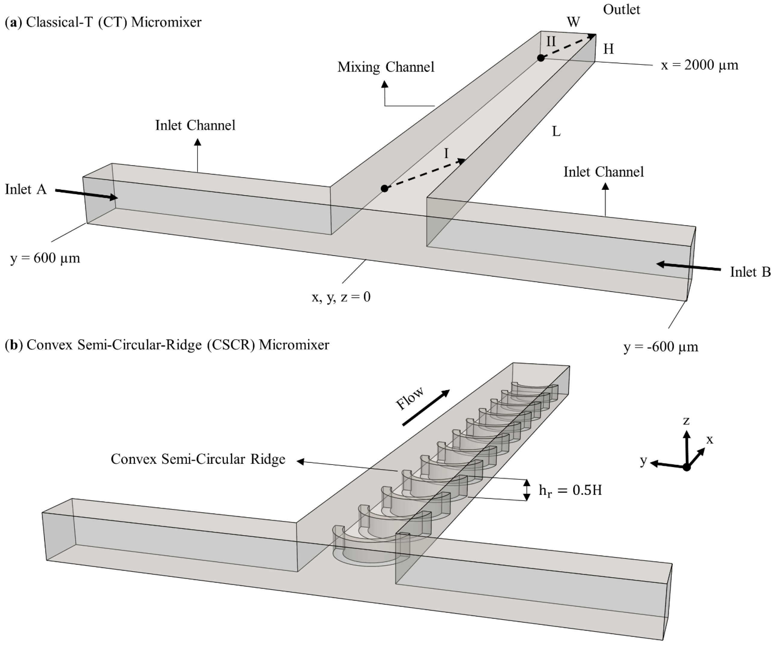Pressure drop in the micromixer, average velocity (ū) on the dashed line arrow I in Figure 1, and mixing index at the outlet.

$$\Delta {\mathrm{D}\left(\mathrm{P}\right)}_{\mathrm{L}\left(\mathrm{i}\right)-\mathrm{L}1}=\left|\frac{P_{L(i)}-P_{L1}}{P_{L1}}\right|\times 100;i=2,3,4,5$$

(6)

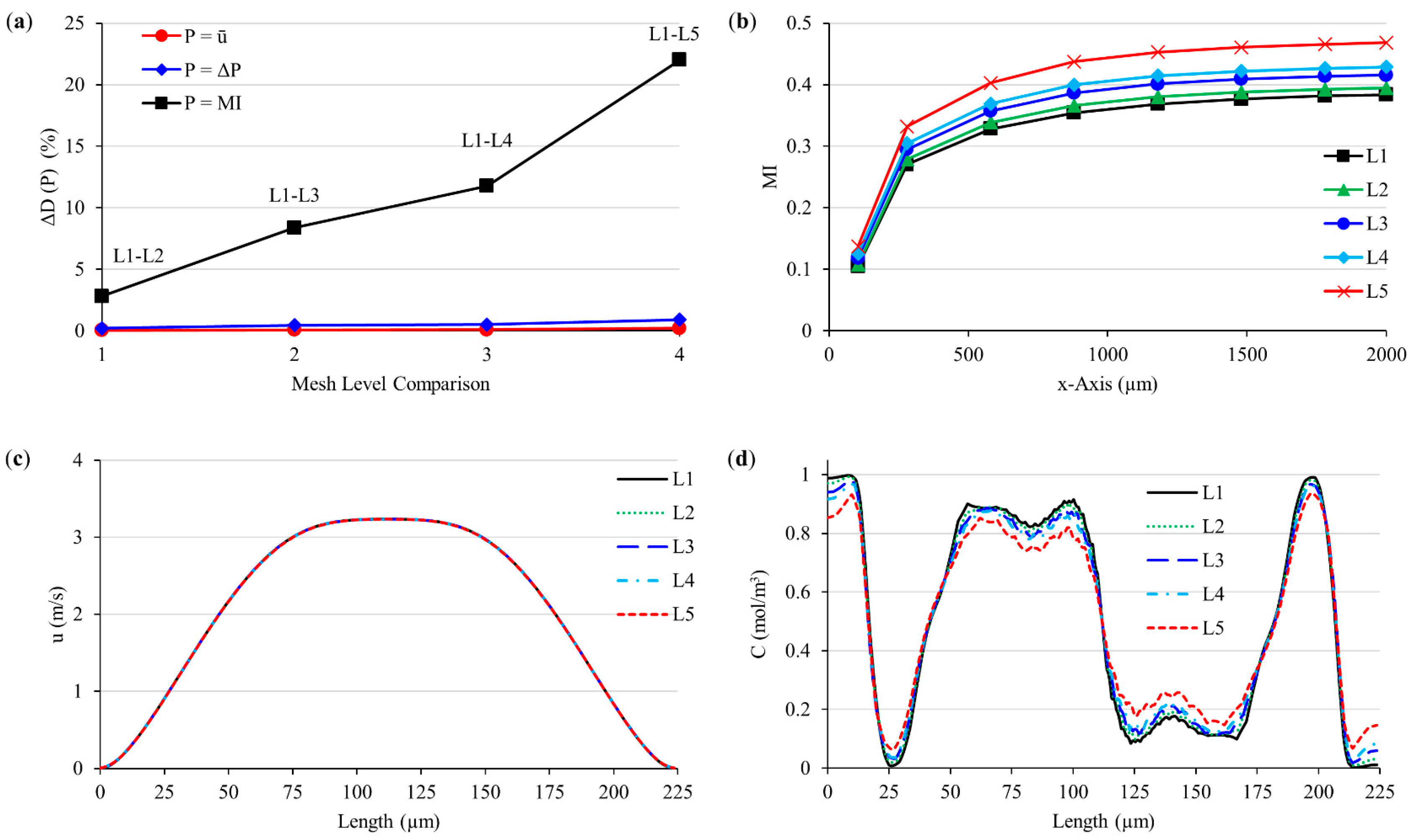
Figure 3a shows that the maximum difference, occurred between L5 and L1 levels, is less than 1% for both flow parameters. According to the trendlines, even the coarsest mesh level is enough to render the flow field quite accurately. However, in contrast to the small Re number in the flow simulation, the transport domain is resolved for a high Pe number, on the order of 8 × 10⁵. When MI parameter is used, the highest difference is observed as 22% between L5 and L1. The peak difference is followed by the values of 11.8%, 8.3%, and 2.8% for other grid level comparisons. Such a big difference between grids emerged as a result of numerical diffusion generation in the solution. In micromixer studies where advective transport inherently prevails, evaluation of flow parameters alone may lead to the reporting of unphysical mixing outcomes. Meanwhile, the development of mixing on several planes along the mixing channel is shown in Figure 3b. In addition, velocity and concentration distributions at the exit (i.e., on the dashed line arrow II in Figure 1) are plotted in Figure 3c,d respectively. As can be seen from the graphs in Figure 3a,b, and Figure 3d, the results obtained from different grid levels, converge to the finest grid. When the top two mesh densities are compared, increasing the element numbers by 3.2 million cause a 2.8% change in the mixing index value. Hence, considering the high computational expense against an insignificant accuracy gain, L2 grid size is selected for the rest of the simulations in this paper. It should be also noted, that the mixing outcomes, obtained in this work, are consistent with the experimental studies in the literature (see the References [39,51]). For instance, Silva et al. [51] investigated a CT-FI-RI configuration experimentally with similar micromixer dimensions and fluid properties employed in this research. Authors reported around 30% and 3.2% mixing efficiency at Re = 256 and 50 respectively. In the present study, the degree of mixing is quantified as 28% and 2.8% for Re = 240 and 40 flow conditions respectively.

5.2. Classical-T (CT) Micromixer

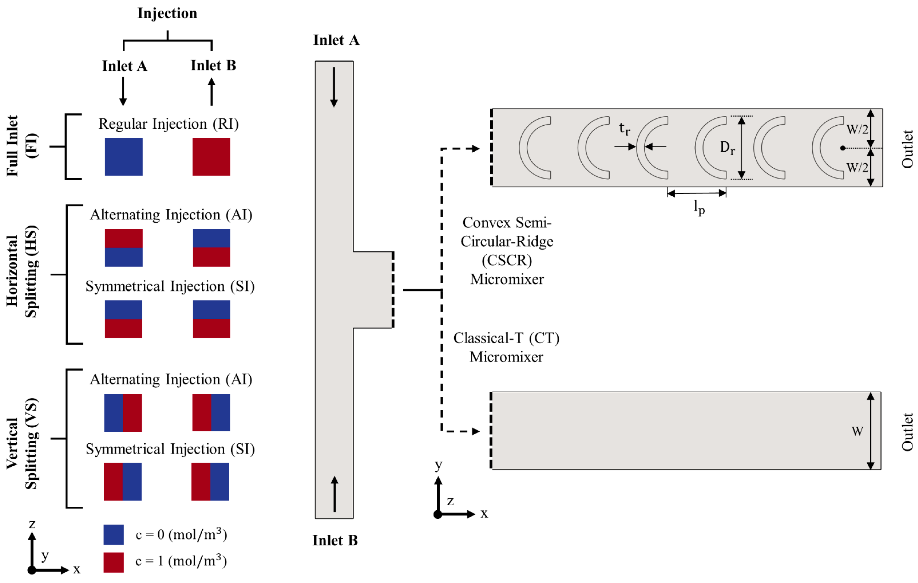
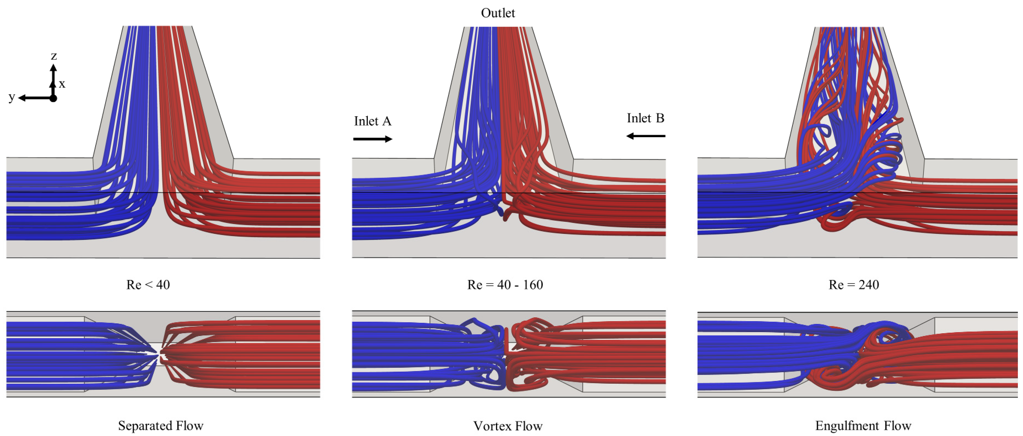
In this section, the mixing characteristics of the CT micromixer is investigated for the entire Re scenarios and molecular diffusion constants given in Table 1. In addition, all inlet types and injection methods in Figure 2 are tested to survey mixing effects. In the CT micromixers, typically following flow regimes develop depending on the flowrate imposed: separated (i.e., segregated), vortex, and engulfment. Figure 4 illustrates the fluid path lines in these flow types with occurrence Re numbers. In a separated flow—which is usually observed in highly laminar flow conditions—fluids, coming from inlets, travel alongside in the mixing channel. In this flow type, fluid bodies create a small contact surface and therefore mixing is completely controlled by molecular diffusion. In vortex flow, however, impingement of streams at the center of the confluence region creates two-counter-rotating vortex pairs in each side of the mixing channel. The periodic movement of fluids relatively increases the contact surface area in comparison with segregated flows. Furthermore, flow type is described as engulfment when the inlet streams partially reach the opposite side of the mixing channel. In engulfment flow, fluid bodies can be stretched, and the contact surface is enlarged higher than that of separated and vortex flow profiles.

Pressure drops and outlet mixing efficiencies—which are obtained from CT-FI-RI micromixer configuration—are plotted in Figure 5a,b respectively. As shown in Figure 5a, while the pressure drop values are less than 1 kPa until Re = 40, the formation of complex flow patterns sharply increases the pressure difference between inlets and outlet. The maximum pressure drop is observed in the engulfment flow regime with a value of slightly over 15 kPa. Mixing indexes, on the contrary, follow a reverse trend with rising flowrates till the highest flow scenario as shown in Figure 5b. In very low Re conditions (e.g., Re = 0.1 and 0.5), relatively high mixing efficiencies are obtained due to long residence time of fluids in the mixing channel. In this case, fluid mixing is purely characterized by diffusive mixing mechanism which is a slow process. Besides, further increase of the Re number yields advection dominant transport conditions where the effect of molecular diffusion is substantially reduced. As a result of diminishing residence times and limited contact surface area formed, mixing indexes continually drop until the Re = 240 flow scenario. Nevertheless, when the engulfment flow pattern is created in the mixing channel, mixing efficiency is mainly enhanced due to the chaotic motion of fluids. In this flow scenario, a mixing index value, around 33%, is obtained at the exit of CT-FI-RI micromixer for all molecular diffusion coefficients, simulated.

The mixing outcomes of the CT-FI-RI micromixer show that secondary flows, developed in the mixing channel, cannot be exploited efficiently. For further investigation of improving the degree of mixing in the CT micromixer, alternative injection types are tested. As shown in Figure 6, multi-injection application contributes to the effective utilization of flow profiles generated in the CT micromixer. While the enhancement of mixing is apparent in separated and vortex flows, split inlets yield quite similar outcomes with the CT-FI-RI configuration at Re = 240. In low Re cases (e.g., Re = 0.1, 0.5, and 1), horizontal and vertical split inlets improve mixing efficiency due to the formation of additional contact layer in inlet channels. In such flow conditions, the amount mixing efficiency is fundamentally determined by the magnitude of molecular diffusion constant. In vortex flow type, however, the enhancement of mixing is mainly affected from splitting type. Namely, while the trendlines continue dropping with increasing Re number in horizontal splitting cases, vertical injection of fluids improves the degree of mixing in cases where Re > 20 (D = D₁). This is basically because vertically travelling fluids in the inlet channels form the upper and lower vortices jointly (see the vortex pairs in each side of the mixing channel in Figure 4). On the contrary, if the flows are aligned horizontally, double vortex pattern is formed separately by top and bottom streams in an inlet channel. The effect of splitting and injection types can be seen in Figure 7, in which outlet concentration distributions are shown. Meanwhile, in both split inlet types, alternating injection presents slightly better mixing values until the engulfment flow case. Such a gain in mixing efficiencies is achieved as a result of extra contact surface, formed between inlet streams along the mixing channel. In engulfment region, however, all the test scenarios yield almost identical mixing efficiencies due to small residence time of fluids in the micromixer. Even though contact surface is inherently larger in alternating injection modes, this is inhibited by relatively short contact time between fluids. Thus, diffusive mixing cannot be utilized effectively, and all splitting and full inlet scenarios provide quite similar mixing results based on advective mixing.

As shown in this section, mixing of fluids in CT micromixers is rather challenging. Despite observing mixing enhancement for multiple injection strategies, the degree of mixing is still far behind the desired levels (e.g., 80%). Particularly, mixing indexes, obtained from the lowest diffusion constant (D₁), are unacceptable for several applications. However, it should be noted that the results, acquired from CT micromixers, are pivotal to understanding flow and transport dynamics in micro-scales and to develop effective alternative designs.

5.3. Convex Semi-Circular-Ridge (CSCR) Micromixer

In passive mixing approach, the development of chaotic advection is essential to achieve well-mixed fluids over a short distance. In this sense, the chaotic advection involves the processes in which fluids are subjected to split, stretch, twist or fold flow configurations. In CT micromixers, chaotic fluid flow is created by vortex and engulfment regimes. However, the deformation of fluid bodies is insufficient to substantially increase the mixing index. Besides, pressure drops, required to form the complex flow patterns, are relatively high as presented in Figure 5. Therefore, the CSCR micromixer is designed to generate an effective chaotic fluid motion under low pressure drop conditions. The novel design is tested for a Re number range between 0.1 and 40. Mixing characteristics are investigated for the split inlet configurations with alternating and symmetrical injections. Additionally, simulations are extended for several diffusion constants to analyze the micromixer under different diffusivity conditions.

In the CSCR micromixer, two counter-rotating, helicoidal-shaped flow profiles are developed along the mixing channel as illustrated in Figure 8. The rotational fluid motion is created employing the stationary semi-circular mixing elements, aligned in the streamwise direction. As a result of effective design factor, the formation of helicoidal patterns starts right after the confluence region and continues along the mixing channel. The semi-circular ridges, which are positioned convexly on the bottom floor of the mixing channel—function to deflect and raise the flows as follows. When the incoming inlet streams reach the first mixing element, fluids, flowing at the height of ridges, i.e., z ≤ 50 µm (see the blue arrow lines in Figure 8), are split and diverted to the gaps, exist between the ridge and side walls of the mixing channel. In this region, the amount of fluid flow is controlled by a small gap size. Accordingly, fluid volume is raised over the gap, and flow continues with a leaning motion towards the center of the mixing channel (i.e., y = 0).

Such an oblique fluid motion is primarily ensured by the convex curvature of the semi-circular ridge. In the meantime, the upper streams, flowing at z > 50 µm (see the red arrow lines in Figure 8), are pushed inwards due to the fluid volume, increased at the edges (see the thick, black arrows). Later, these streams are split and diverted to the side walls by the following ridges in the mixing channel. It should be pointed out here that the symmetrical, leaning flows converge at the center of the mixing channel (y = 0) after flowing over the next several ridges (see the pathlines in Figure 8). By this way, straight fluid flow, above the obstructions, is blocked in the streamwise direction. So that the upper streams are intrinsically forced to use the paths between consecutive ridges. In the same way, fluids are raised over the gaps and follow the same oblique path towards the center of the mixing channel. The formation of rotational fluid flow along the mixing channel can be also tracked from Figure 9 which shows concentration distributions along the mixing channel of CSCR-VS-AI configuration (D = D₁). Rotational fluid motion is observed even at the smallest flow case tested (i.e., Re = 0.1). In addition, the frequency of rotations is improved with increasing Re number.

The maximum flow scenario is chosen as Re = 40 for the CSCR micromixer simulations. It is clear from the trend shown in Figure 9 that the chaotic behavior of fluid flow and therefore fluid mixing improve with rising Re. Further increase of Re after Re = 40 will increase the intensity of rotations and provide better mixing efficiencies with a cost of higher pressure drop and thus energy requirement. For the Re = 40 case, an effective chaotic fluid flow has yielded a mixing efficiency value greater than 80% with a feasible pressure drop. As a result of the small form factor of the semi-circular ridges, the CSCR micromixer produces the helicoidal fluid motion resulting in low pressure drops. As shown in Figure 10, the pressure drops are obtained as 2.07 and 4.72 kPa at Re = 20 and 40 flow scenarios respectively. When these values are compared with the outcomes of micromixers, reviewed in the introduction section, the energy requirement of the CSCR micromixer is far less than that of reported in the literature.

Meanwhile, mixing results indicate that alternating and symmetrical injection modes provide parallel mixing outcomes as shown in Figure 11. Similar mixing efficiencies are observed as a result of intermittent contact time between two flow profiles in the mixing channel. Namely, diffusive interaction between the counter-rotating, helicoidal-shaped flows is quite limited due to ongoing rotations.

Therefore, the additional contact surface area, which is formed at the center of the mixing channel (y = 0) in alternating injection mode, cannot be utilized pointedly. The type of splitting, however, affects the utilization of the chaotic flow profile as illustrated in Figure 12. In the mixing channel, the distribution of concentration differs with the splitting type. During the development of the helicoidal-shaped profile, the regions, above (z > 50 µm) and below (z ≤ 50 µm) the mixing elements, are fed dissimilarly depending on the splitting type. While the horizontal split inlets deliver a different fluid (c = 0 or 1 mol/m³) to each region, the vertical split inlets feed the upper and lower sections with a fluid pair (c = 0 and 1 mol/m³). Hence, in comparison to the horizontal type, the use of vertical split inlets forms a relatively high contact surface. Besides, the lowest mixing outcomes are obtained when the CSCR micromixer is operated in FI-RI mode. Since each of the helicoidal flows is generated separately by the fluids coming from inlet A and B as shown in Figure 8, the only contact surface is formed between counter-rotating fluid bodies along the center of the mixing channel (y = 0). In this case, the CSCR-FI-RI design is reduced to the CT-FI-RI micromixer. Both configurations yield almost identical mixing efficiencies and concentration distributions as presented in Figure 5b and Figure 7 respectively (see the outcomes of the CT-FI-RI for Re = 0.1–40). Thus, the active utilization of the helicoidal flows is primarily controlled by the horizontal or vertical feeding type of the CSCR micromixer.

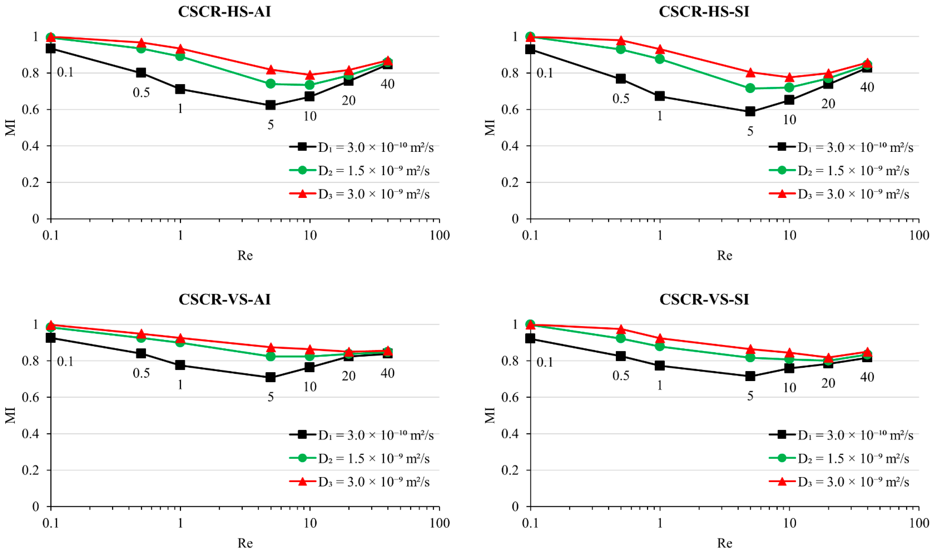
When the CSCR-HS-AI and CSCR-VS-AI configurations are compared, vertical split inlet provides higher mixing index values for the Re numbers between 0.5 and 20. The minimum and maximum variances are observed as 4.7% and 12.3% at Re = 0.5 and 10 flow conditions respectively (D = D₁). Based on the differences calculated, the effect of additional fluid pair is more prominent in the transition region, i.e., Re = 1–10. Besides, equal amount of mixing efficiency is obtained for all diffusion constants at Re = 0.1 and 40. In the slowest flow case, the efficiency of mixing is primarily controlled by the diffusive mixing. The extent of contact surface area in micromixer configurations is substantially suppressed by the high residence time of fluids. After Re = 0.1, the function of molecular diffusion diminishes with decreasing fluid residence times. This is quite evident from the deviating trendlines of the smallest diffusion coefficient until Re = 5. After this flow case, the intensity of rotational flow profile is enhanced with rising flowrates. Trendlines show a convergent behavior due to developing complex flow patterns and lessening diffusion effects. Notably, diffusive mixing becomes negligible when the highest flow condition is reached. Fluids are mainly mixed based on the chaotic flow profile formed. Therefore, the same amount of mixing efficiency is obtained at Re = 40 regardless of the diffusion magnitudes. In all configurations, the minimum mixing index is obtained at Re = 5 flow scenario (D = D₁). At this pivotal point, the degree of mixing is mostly controlled by the chaotic advection. The smallest diffusion constant yields 62% and 71% mixing efficiency in the CSCR-HS-AI and CSCR-VS-AI setups respectively. Meanwhile, the maximum mixing value in each Re case is usually provided by the CSCR-VS-AI configuration. In most cases more than 80% homogenous fluid mixing is obtained. In highly laminar flow regimes, mixing indexes are computed to be 92% and 84% for Re = 0.1 and 0.5 respectively (D = D₁). 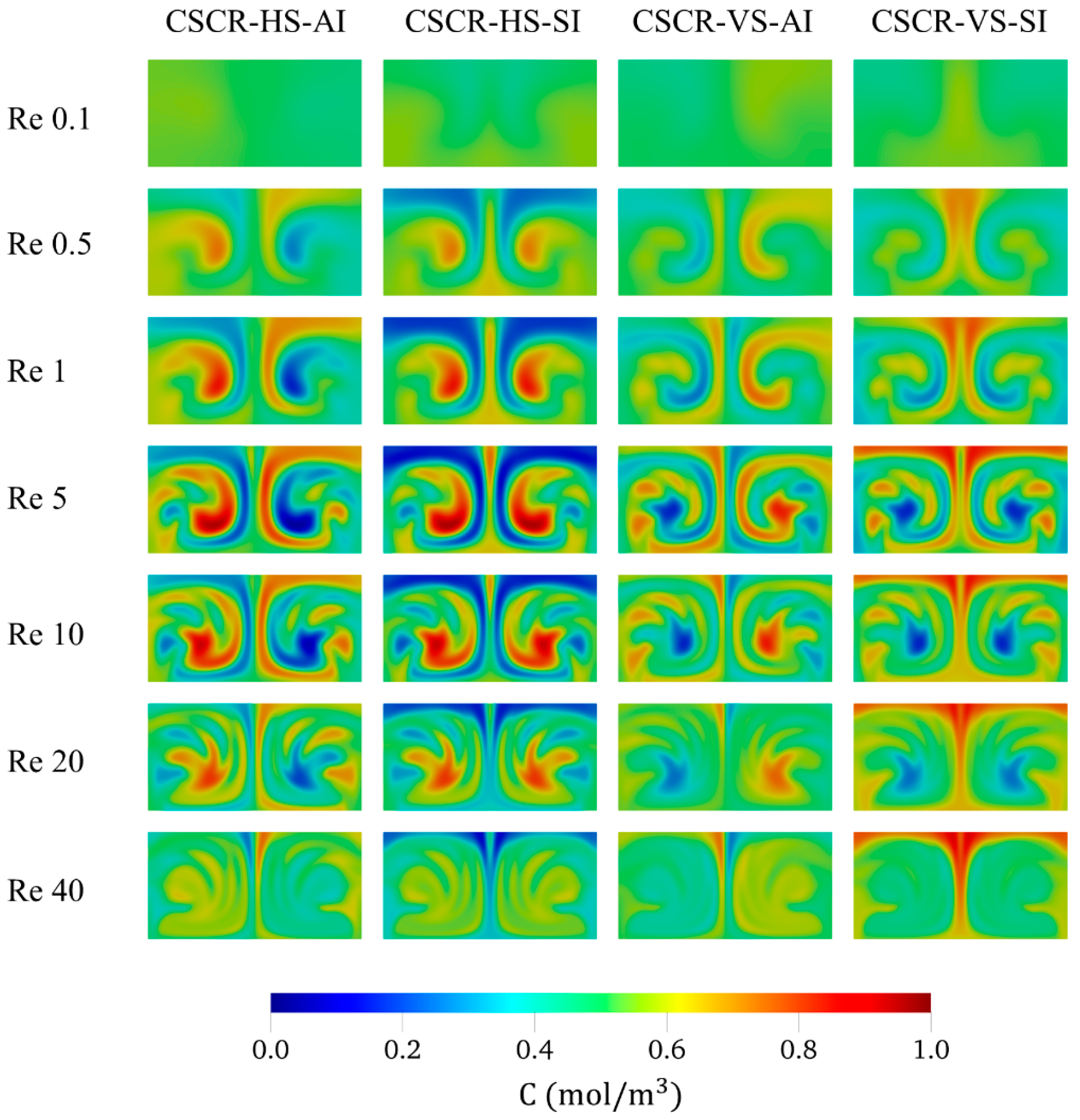Relatively low mixing efficiencies are observed in the transition region, i.e., Re = 1–10 (D = D₁). The degree of mixing is quantified as 78% and 76.4% for Re = 1 and 10 respectively. Furthermore, nearly 83% and 85% mixing index is computed in the two most chaotic flow conditions respectively, i.e., Re = 20 and 40. Outlet concentration distributions of the CSCR micromixer configurations are shown in Figure 13.

The CSCR micromixer activates an effective, chaotic fluid flow with rising flowrates. Especially, in the flow cases where Re = 20 and 40, fluid mixing is predominantly carried out based on strong deformation of fluid bodies. In other flow conditions, however, diffusive mixing affects the degree of mixing at different rates depending on the following factors: magnitude of molecular diffusion coefficient, fluid residence time, and the contact surface between fluids. The most challenging mixing conditions are observed in Re = 1, 5, and 10 scenarios when the molecular diffusion constant is too small (i.e., D = D₁). Shortening residence time of fluids substantially inhibits the function of diffusivity whereas the contact surface is enlarged. Accordingly, fluids are largely mixed depending on the deformation rate of fluids in the rotations. Besides, in relatively high laminar flow region, i.e., Re = 0.1 and 0.5, diffusive interaction is amplified due to high contact time over the contact surfaces of fluid bodies. Therefore, the mixing of fluids is primarily conducted by diffusive mixing.

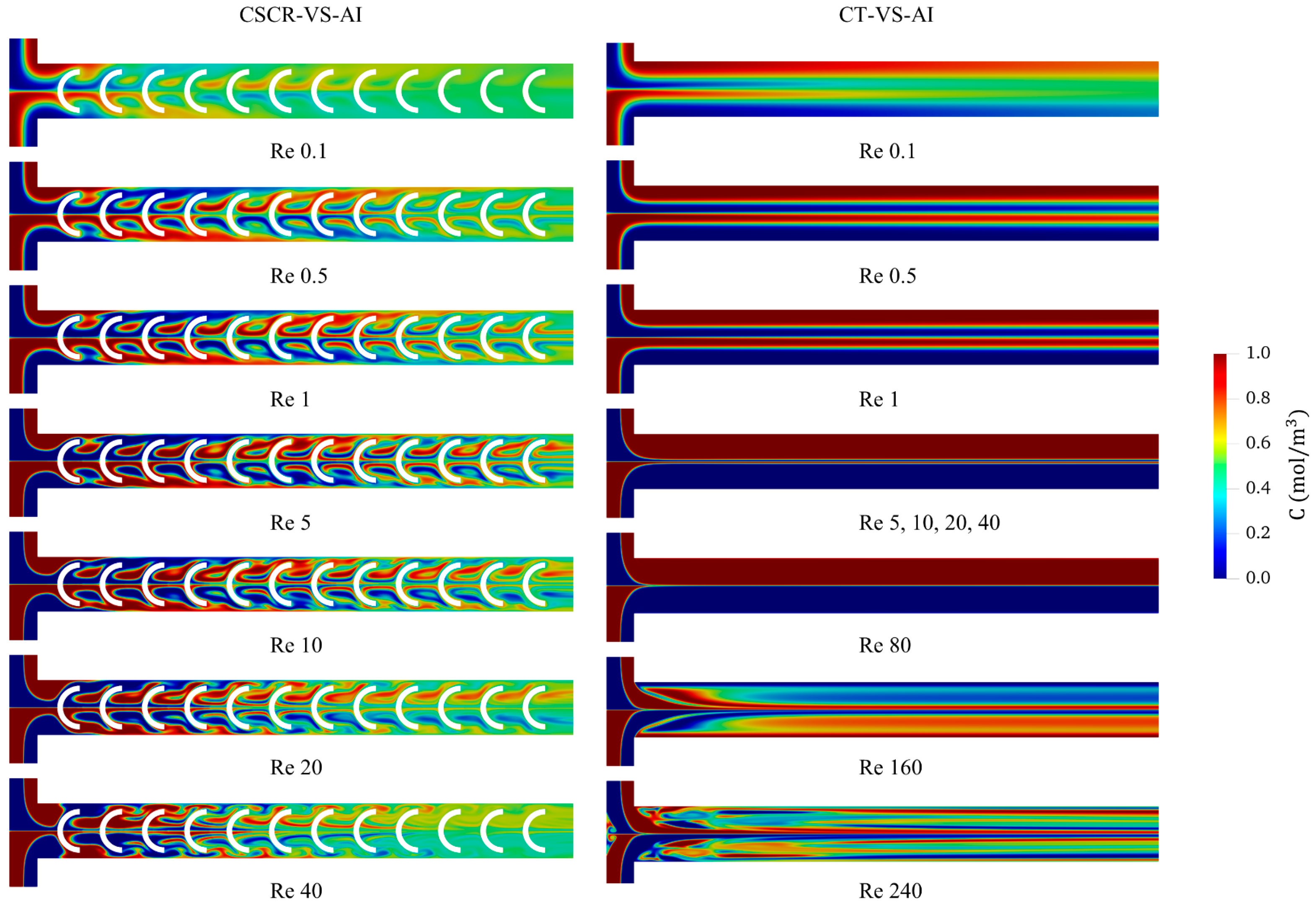
In Figure 14a,b, the CSCR and CT micromixers are compared in terms of mixing efficiency and mixing performance. Vertical split inlets and alternating injection configurations are considered for both micromixers. Accordingly, only the effect of semi-circular ridges, in convex position, is highlighted. Bar charts are obtained normalizing the outcomes of the CSCR-VS-AI by that of the CT-VS-AI. In addition, concentration distributions on the x-y plane at the middle height (i.e., z = 50 µm) of the CSCR-VS-AI and CT-VS-AI micromixers are shown in Figure 15 (D = D₁).

Figure 14a indicates that the efficiency of mixing is substantially increased over the CT micromixer. The maximum improvement is observed for the smallest molecular diffusion coefficient tested because fluid mixing is primarily carried out based on the chaotic action. In highly laminar flow region, the ratios are found to be 1.23 and 2 for Re = 0.1 and 0.5 respectively (D = D₁). The degree of mixing is enhanced up to 7.3 times over the CT design under the toughest mixing conditions, i.e., Re = 1–10. In the most chaotic region, however, the CSCR micromixer provides around 8.7 times higher mixing values. When the pressure drops are evaluated, comparatively lower ratios are obtained for mixing performance. The maximum ratio is observed as 3.3 at Re = 20. In the CSCR design, higher pressure drops are yielded as a result of mixing channel cross-section, confined by ridges. However, it should be noted that all the energy, spend in the CSCR micromixer, is utilized to form a rotational fluid motion. In contrast, CT micromixer results in lower pressure drops due to a smooth, segregated flow profile developed in the unobstructed mixing channel.

Meanwhile, the increase in mixing efficiency and mixing performance slows down with increasing diffusion magnitudes. Besides, the lowest ratios are observed in the highly laminar flow region (i.e., Re = 0.1, 0.5, and 1) as can be seen in Figure 14a,b. First and foremost, the scarce contact time of fluids in the CSCR micromixer cause to yield lower ratios. Namely, fluid particles travel much faster in the CSCR micromixer as a result of mixing channel cross-section restricted. This can be seen in Figure 6 and Figure 11. Trendlines, belong to different diffusion constants, converge at Re = 20 and 160 in the CSCR-VS-AI and CT-VS-AI configurations respectively. Therefore, diffusive effects become more prominent in CT micromixer. Second, the CSCR micromixer develop higher mixing efficiencies in a shorter distance as shown in Figure 14c,d. Mixing length reduces when the magnitude of diffusion coefficient is increased. Correspondingly, the actual pressure drops lessen when the number of mixing elements is reduced. Therefore, the ratios will increase in cases that the design outcomes are compared before the exit of the micromixers.

5.4. Alternative Micromixer Configurations

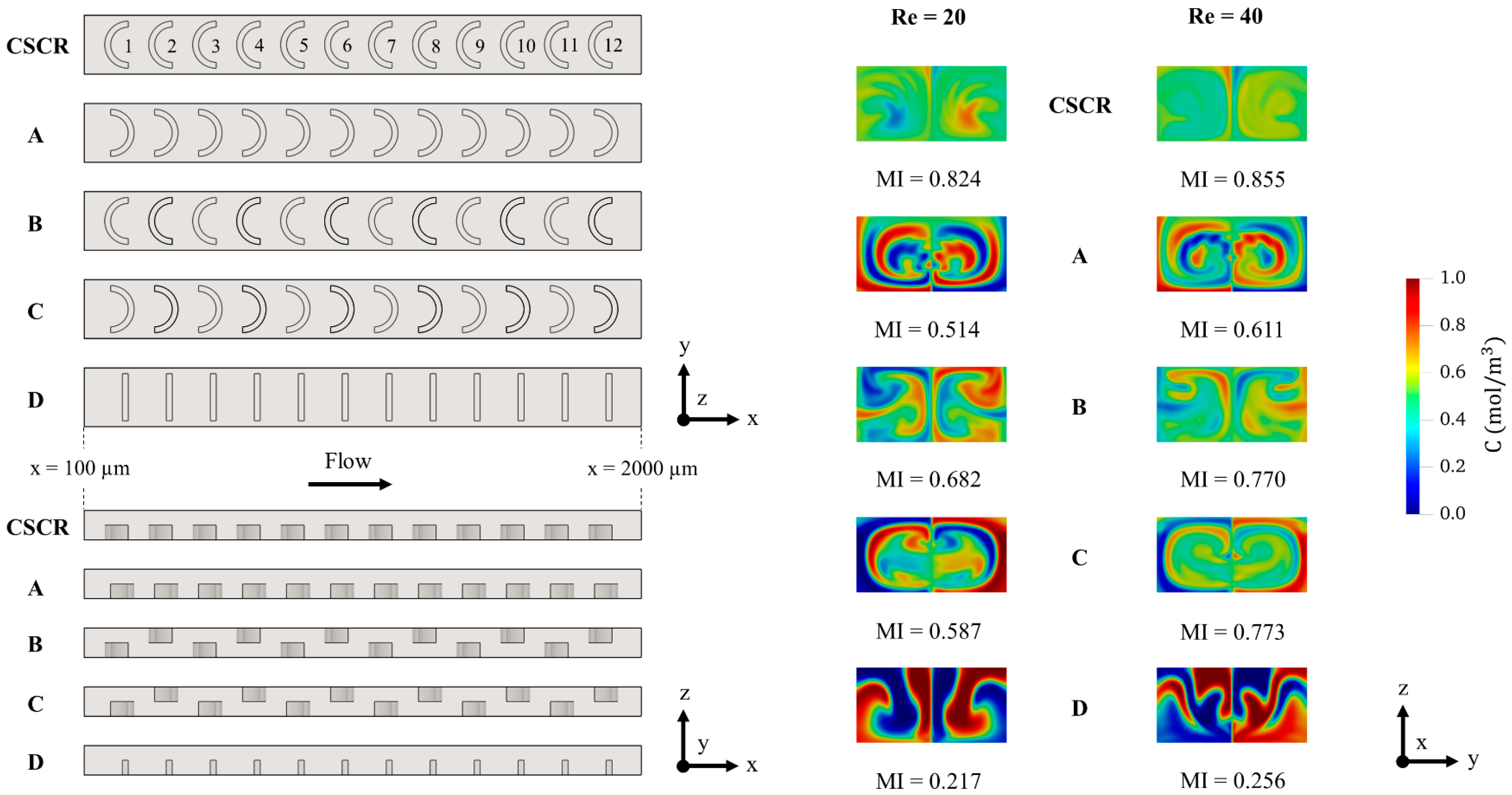
In the present study, alternative micromixer configurations are also examined as schematically shown in Figure 16. The same geometrical dimensions are preserved in A, B, C and D designs with that of the CSCR micromixer (i.e., L, W, H, h_r, D_r, t_r, and l_p). In the A, B, and C configurations, the different positioning effects of the semi-circular ridges are surveyed. In the design A, the mixing elements are positioned concavely on the bottom floor of the mixing channel. The same objects, however, are arranged as baffles with convex and concave orientations in the designs B and C respectively. In both setups, odd- and even-numbered ridges are located on the bottom and top floors of the mixing channel respectively. Besides, the effect of rectangular ridges, which are aligned on the bottom floor of the mixing channel, is investigated in the design D. All configurations are tested in the two most chaotic flow region, i.e., Re = 20 and 40, with vertical split inlets and alternating injection mode. Simulations are conducted for the smallest diffusion constant (D = D₁) aiming to reveal the actual mixing characteristics based on the chaotic advection. The degree of mixing is quantified for each flow condition and presented along with outlet concentration distributions in Figure 16.

As given in Figure 16, the lowest mixing outcomes are obtained when rectangular ridges are employed (i.e., case D). Inlet streams predominantly flow around the central part of the mixing channel (y = 0) with slight fluctuations in the z-direction. Fluids, coming from the outer sub-inlets (i.e., red and blue colors at the center of the outlet cross-section), are partially diverted to the gaps at the first inlet. After this point, fluid flow is maintained above the gap area over several mixing elements. A slanting fluid motion is observed towards the center of the mixing channel (y = 0) around the sixth element, and it is kept until the exit. Therefore, a rather limited distortion occurred in fluid bodies. In the concave position of the semi-circular elements (i.e., case A), inlet streams are largely deflected to the center of the mixing channel (y = 0) due to inwards curvature of the ridges. As opposed to the convex orientation, fluid volumes are mostly raised at the center of the mixing elements. Later, two symmetrical, leaning flow patterns are followed towards the side channels of the mixing channel. In the meantime, fluids, in the gap regions, followed a path between consecutive ridges and merged with the mainstream, flowing at the center of the mixing channel (y = 0). Even though a rotational fluid behavior is observed, the alternation rates of fluid bodies are much lower than that of the CSCR micromixer. Meanwhile, baffle-type arrangements mixed the fluids without developing a periodic fluid flow in the mixing channel. Inlet streams are mixed intermittently by the mixing elements, located on the bottom and top floors. Fluid bodies are stretched and deflected depending on the position of the semi-circular elements. In convex and concave positions of the semi-circular ridges, fluid bodies are manipulated similarly by each mixing element as described in the CSCR and A configurations respectively. In the baffle-type setups, however, leaning motions are created in the +z- and −z-direction by odd- and even-numbered mixing elements respectively. Although a chaotic fluid flow is also created in the B and C configurations, distortion of fluids is considerably lower than that of the CSCR micromixer.

As shown in this study, the convex alignment of the semi-circular ridges yields a specific, helicoidal-shaped flow pattern. Compared to the alternative configurations, the highest deformation rate of fluid bodies is observed in the CSCR micromixer. The design dynamics develop an effective, chaotic flow state in a flow condition as low as Re = 20. In most cases simulated, well-mixed state of fluids with homogenous concentration distributions is reached in a distance less than 2000 µm as shown in Figure 14c,d. It should be noted that the effects of several parameters in the CSCR micromixer are also investigated which we do not report in the paper. The dimensions, given for semi-circular ridges (i.e., h_r, D_r, t_r, and l_p), are found to be optimum values to yield the maximum mixing efficiency. Further increase or decrease of these parameters, negatively affected the intensity of the rotational fluid motion developed, and therefore the degree of mixing. Besides, double inlet channel has been employed in the CSCR design to be consistent with the CT micromixer. A similar helicoidal-shaped flow is also obtained with a single inlet channel—resulting in higher pressure drop for the same Re condition—positioned in the streamwise direction at the beginning of the mixing channel.

6. Conclusions

In this paper, 3-D T-shaped passive micromixers are studied numerically and a novel micromixer configuration is proposed. Mixing characteristics are investigated under several fluid flow and transport conditions. The effects of alternative inlet splitting, and injection strategies are examined. It was shown that the unobstructed classical-T micromixer develops chaotic fluid motion when Re number is greater than 40. However, the effect of complex flow patterns was rather limited to raise the degree of fluid mixing significantly. A mixing enhancement was observed in the engulfment flow type regardless of the inlet type, injection mode, and the magnitude of diffusion coefficient. Besides, inlet splitting helped to improve fluid mixing in vortex regimes, but the contribution of split inlets was more prominent in low Re number conditions.

The novel passive micromixer was designed employing semi-circular ridges. It was revealed that the alignment of ridges in convex position yields a specific, helicoidal-shaped fluid flow. The chaotic behavior of fluids was observed in a Re range between 0.1 and 40. The intensity of rotations was boosted with growing flowrates. The maximum mixing results were obtained with vertical split inlets and alternating injection mode. In most cases simulated, more than 80% homogenous mixing efficiency was obtained. Well-mixed state of fluids was reached in a distance less than 2000 µm. Pressure drops were computed as 2.07 and 4.72 kPa in the two highest flow conditions respectively, i.e., Re = 20 and 40. The outcomes of the CSCR micromixer were found to be far beyond the passive micromixer designs that are reported in the literature. In comparison with the classical-T micromixer, the novel design increased mixing efficiency and mixing performance by the factors of 8.7 and 3.3 respectively.

Furthermore, alternative micromixer configurations were assessed. It was found that the use of rectangular ridges resulted in several times lower mixing index than the CSCR micromixer. In addition, although the concave positioning and baffle-type arrangements enhanced mixing efficiency, the deformation rate of fluid bodies was lower than that of the CSCR micromixer. Consequently, the CSCR passive micromixer was proposed for microfluidic systems where a rapid and thorough fluid mixing is needed.

References

1. Lee, C.-Y.; Wang, W.-T.; Liu, C.-C.; Fu, L.-M. Passive mixers in microfluidic systems: A review. Chem. Eng. J. 2016, 288, 146–160. [Google Scholar] [CrossRef]
2. Mansur, E.A.; Ye, M.; Wang, Y.; Dai, Y. A State-of-the-Art Review of Mixing in Microfluidic Mixers. Chin. J. Chem. Eng. 2008, 16, 503–516. [Google Scholar] [CrossRef]
3. Ward, K.; Fan, Z.H. Mixing in microfluidic devices and enhancement methods. J. Micromech. Microeng. 2015, 25. [Google Scholar] [CrossRef] [PubMed]
4. Schonfeld, F.; Hessel, V.; Hofmann, C. An optimised split-and-recombine micro-mixer with uniform chaotic mixing. Lab Chip 2004, 4, 65–69. [Google Scholar] [CrossRef] [PubMed]
5. Kumar, V.; Paraschivoiu, M.; Nigam, K.D.P. Single-phase fluid flow and mixing in microchannels. Chem. Eng. Sci. 2011, 66, 1329–1373. [Google Scholar] [CrossRef]
6. Reyes, D.R.; Iossifidis, D.; Auroux, P.-A.; Manz, A. Micro Total Analysis Systems. 1. Introduction, Theory, and Technology. Anal. Chem. 2002, 74, 2623–2636. [Google Scholar] [CrossRef] [PubMed]
7. Aubin, J.; Ferrando, M.; Jiricny, V. Current methods for characterising mixing and flow in microchannels. Chem. Eng. Sci. 2010, 65, 2065–2093. [Google Scholar] [CrossRef]
8. Nguyen, N.-T.; Wu, Z. Micromixers—A review. J. Micromech. Microeng. 2005, 15, R1–R16. [Google Scholar] [CrossRef]
9. Suh, Y.K.; Kang, S. A Review on Mixing in Microfluidics. Micromachines 2010, 1, 82–111. [Google Scholar] [CrossRef]
10. Gambhire, S.; Patel, N.; Gambhire, G.; Kale, S. A review on different micromixers and its micromixing within microchannel. Int. J. Curr. Eng. Technol. 2016, 4, 409–413. [Google Scholar]
11. Capretto, L.; Cheng, W.; Hill, M.; Zhang, X. Micromixing within microfluidic devices. Top. Curr. Chem. 2011, 304, 27–68. [Google Scholar] [CrossRef] [PubMed]
12. Cai, G.; Xue, L.; Zhang, H.; Lin, J. A Review on Micromixers. Micromachines 2017, 8, 274. [Google Scholar] [CrossRef] [PubMed]
13. Gidde, R.R.; Pawar, P.M. Flow feature and mixing performance analysis of RB-TSAR and EB-TSAR micromixers. Microsyst. Technol. 2019. [Google Scholar] [CrossRef]
14. Park, J.M.; Seo, K.D.; Kwon, T.H. A chaotic micromixer using obstruction-pairs. J. Micromech. Microeng. 2009, 20, 015023. [Google Scholar] [CrossRef]
15. Gidde, R.R.; Pawar, P.M.; Ronge, B.P.; Misal, N.D.; Kapurkar, R.B.; Parkhe, A.K. Evaluation of the mixing performance in a planar passive micromixer with circular and square mixing chambers. Microsyst. Technol. 2017. [Google Scholar] [CrossRef]
16. Lee, C.Y.; Chang, C.L.; Wang, Y.N.; Fu, L.M. Microfluidic mixing: A review. Int. J. Mol. Sci. 2011, 12, 3263–3287. [Google Scholar] [CrossRef] [PubMed]
17. Chung, Y.-C.; Hsu, Y.-L.; Jen, C.-P.; Lu, M.-C.; Lin, Y.-C. Design of passive mixers utilizing microfluidic self-circulation in the mixing chamber. Lab Chip 2004, 4, 70–77. [Google Scholar] [CrossRef]
18. Rudyak, V.Y.; Minakov, A.V.; Gavrilov, A.A.; Dekterev, A.A. Modelling of flows in micromixers. Thermophys. Aeromech. 2010, 17, 565–576. [Google Scholar] [CrossRef]
19. Li, L. Design of Micromixer and Microfluidic Control System. Ph.D. Thesis, Florida Atlantic University, Boca Raton, FL, USA, 2013. [Google Scholar]
20. Bhopte, S.; Sammakia, B.; Murray, B. Geometric modifications to simple microchannel design for enhanced mixing. In Proceedings of the 2008 11th Intersociety Conference on Thermal and Thermomechanical Phenomena in Electronic Systems, Orlando, FL, USA, 28–31 May 2008; pp. 937–944. [Google Scholar]
21. Le The, H.; Le Thanh, H.; Dong, T.; Ta, B.Q.; Tran-Minh, N.; Karlsen, F. An effective passive micromixer with shifted trapezoidal blades using wide Reynolds number range. Chem. Eng. Res. Des. 2015, 93, 1–11. [Google Scholar] [CrossRef]
22. Bhopte, S.; Sammakia, B.; Murray, B. Numerical study of a novel passive micromixer design. In Proceedings of the 2010 12th IEEE Intersociety Conference on Thermal and Thermomechanical Phenomena in Electronic Systems, Las Vegas, NV, USA, 2–5 June 2010; pp. 1–10. [Google Scholar]
23. Cortes-Quiroz, C.A.; Azarbadegan, A.; Zangeneh, M. Evaluation of flow characteristics that give higher mixing performance in the 3-D T-mixer versus the typical T-mixer. Sens. Actuators B Chem. 2014, 202, 1209–1219. [Google Scholar] [CrossRef] [Green Version]
24. Fang, Y.; Ye, Y.; Shen, R.; Zhu, P.; Guo, R.; Hu, Y.; Wu, L. Mixing enhancement by simple periodic geometric features in microchannels. Chem. Eng. J. 2012, 187, 306–310. [Google Scholar] [CrossRef]
25. Wong, S.H.; Bryant, P.; Ward, M.; Wharton, C. Investigation of mixing in a cross-shaped micromixer with static mixing elements for reaction kinetics studies. Sens. Actuators B Chem. 2003, 95, 414–424. [Google Scholar] [CrossRef]
26. Afzal, A.; Kim, K.-Y. Passive split and recombination micromixer with convergent–divergent walls. Chem. Eng. J. 2012, 203, 182–192. [Google Scholar] [CrossRef]
27. Alam, A.; Afzal, A.; Kim, K.-Y. Mixing performance of a planar micromixer with circular obstructions in a curved microchannel. Chem. Eng. Res. Des. 2014, 92, 423–434. [Google Scholar] [CrossRef]
28. Shih, T.R.; Chung, C.K. A high-efficiency planar micromixer with convection and diffusion mixing over a wide Reynolds number range. Microfluid. Nanofluid. 2007, 5, 175–183. [Google Scholar] [CrossRef]
29. Tran-Minh, N.; Dong, T.; Karlsen, F. An efficient passive planar micromixer with ellipse-like micropillars for continuous mixing of human blood. Comput. Methods Programs Biomed. 2014, 117, 20–29. [Google Scholar] [CrossRef]
30. Chung, C.K.; Shih, T.R. A rhombic micromixer with asymmetrical flow for enhancing mixing. J. Micromech. Microeng. 2007, 17, 2495–2504. [Google Scholar] [CrossRef]
31. Xu, Z.; Li, C.; Vadillo, D.; Ruan, X.; Fu, X. Numerical simulation on fluid mixing by effects of geometry in staggered oriented ridges micromixers. Sens. Actuators B Chem. 2011, 153, 284–292. [Google Scholar] [CrossRef]
32. Wang, L.; Liu, D.; Wang, X.; Han, X. Mixing enhancement of novel passive microfluidic mixers with cylindrical grooves. Chem. Eng. Sci. 2012, 81, 157–163. [Google Scholar] [CrossRef]
33. Hossain, S.; Kim, K.-Y. Numerical Study on Mixing Performance of Straight Groove Micromixers. Int. J. Fluid Mach. Syst. 2010, 3, 227–234. [Google Scholar] [CrossRef]
34. Wang, L.; Yang, J.-T.; Lyu, P.-C. An overlapping crisscross micromixer. Chem. Eng. Sci. 2007, 62, 711–720. [Google Scholar] [CrossRef]
35. Ansari, M.A.; Kim, K.-Y. Shape optimization of a micromixer with staggered herringbone groove. Chem. Eng. Sci. 2007, 62, 6687–6695. [Google Scholar] [CrossRef]
36. Jian Chen, J.; Ren Lai, Y.; Tang Tsai, R.; Der Lin, J.; Yang Wu, C. Crosswise ridge micromixers with split and recombination helical flows. Chem. Eng. Sci. 2011, 66, 2164–2176. [Google Scholar] [CrossRef]
37. Sabotin, I.; Tristo, G.; Junkar, M.; Valentinčič, J. Two-step design protocol for patterned groove micromixers. Chem. Eng. Res. Des. 2013, 91, 778–788. [Google Scholar] [CrossRef]
38. Izadpanah, E.; Hekmat, M.H.; Azimi, H.; Hoseini, H.; Babaie Rabiee, M. Numerical simulation of mixing process in T-shaped and DT-shaped micromixers. Chem. Eng. Commun. 2018, 205, 363–371. [Google Scholar] [CrossRef]
39. Bothe, D.; Stemich, C.; Warnecke, H.-J. Fluid mixing in a T-shaped micro-mixer. Chem. Eng. Sci. 2006, 61, 2950–2958. [Google Scholar] [CrossRef]
40. Soleymani, A.; Kolehmainen, E.; Turunen, I. Numerical and experimental investigations of liquid mixing in T-type micromixers. Chem. Eng. J. 2008, 135, S219–S228. [Google Scholar] [CrossRef]
41. Galletti, C.; Roudgar, M.; Brunazzi, E.; Mauri, R. Effect of inlet conditions on the engulfment pattern in a T-shaped micro-mixer. Chem. Eng. J. 2012, 185, 300–313. [Google Scholar] [CrossRef]
42. Roudgar, M.; Brunazzi, E.; Galletti, C.; Mauri, R. Numerical Study of Split T-Micromixers. Chem. Eng. Technol. 2012, 35, 1291–1299. [Google Scholar] [CrossRef]
43. Ansari, M.A.; Kim, K.-Y.; Anwar, K.; Kim, S.M. Vortex micro T-mixer with non-aligned inputs. Chem. Eng. J. 2012, 181, 846–850. [Google Scholar] [CrossRef]
44. Wang, D.; Ba, D.; Liu, K.; Hao, M.; Gao, Y.; Wu, Z.; Mei, Q. A Numerical Research of Herringbone Passive Mixer at Low Reynold Number Regime. Micromachines 2017, 8, 325. [Google Scholar] [CrossRef] [PubMed]
45. Okuducu, M.B.; Aral, M.M. Computational Evaluation of Mixing Performance in 3-D Swirl-Generating Passive Micromixers. Processes 2019, 7, 121. [Google Scholar] [CrossRef]
46. Okuducu, M.B.; Aral, M.M. Performance Analysis and Numerical Evaluation of Mixing in 3-D T-Shape Passive Micromixers. Micromachines 2018, 9, 210. [Google Scholar] [CrossRef] [PubMed]
47. OpenFOAM. The OpenFOAM Foundation, v5; OpenCFD Ltd.: Bracknell, UK, 2015. [Google Scholar]
48. Warming, R.F.; Beam, R.M. Upwind Second-Order Difference Schemes and Applications in Aerodynamic Flows. AIAA J. 1976, 14, 1241–1249. [Google Scholar] [CrossRef]
49. Zhang, M.; Wu, J.; Wang, L.; Xiao, K.; Wen, W. A simple method for fabricating multi-layer PDMS structures for 3D microfluidic chips. Lab Chip 2010, 10, 1199–1203. [Google Scholar] [CrossRef] [PubMed]
50. Chen, X. Fabrication and performance evaluation of two multi-layer passive micromixers. Sens. Rev. 2018, 38, 321–325. [Google Scholar] [CrossRef]
51. Silva, J.P.; Dos Santos, A.; Semiao, V. Experimental characterization of pulsed Newtonian fluid flows inside T-shaped micromixers with variable inlets widths. Exp. Therm. Fluid Sci. 2017, 89, 249–258. [Google Scholar] [CrossRef]
Figure 1. 3-D micromixer geometries (a) Classical-T (CT) micromixer; (b) Convex semi-circular-ridge (CSCR) micromixer. Diagonal dashed line arrows I and II are on the y-z plane at x = 100 and 2000 µm, respectively.
Processes 07 00637 g001
Figure 2. Inlet types, injection modes and 2-D micromixer geometries.
Processes 07 00637 g002
Figure 3. Grid study outcomes: (a) difference (%) between mesh levels for the parameters tested; (b) development of mixing on different y-z cross-sections along the mixing channel; (c,d) velocity and concentration distributions at the exit respectively (dashed line arrow II in Figure 1).
Processes 07 00637 g003
Figure 4. Flow regimes in the CT micromixer: separated, vortex, and engulfment. Blue and red colors are used to differentiate flow pathlines in inlets A and B.
Processes 07 00637 g004
Figure 5. (a) Pressure drop vs. Re number in CT micromixer. The numbers before and after the semicolons represent Re number and pressure drop values respectively; (b) MI vs. Re number for different molecular diffusion coefficients in CT-FI-RI.
Processes 07 00637 g005
Figure 6. MI vs. Re for three different molecular diffusion constants and four CT micromixer configurations.
Processes 07 00637 g006
Figure 7. Outlet concentration distributions in CT micromixer configurations for D1 = 3.0 × 10⁻¹⁰ m2/s molecular diffusion constant.
Processes 07 00637 g007
Figure 8. Helicoidal fluid flow in the mixing channel at Re = 40. Yellow and green colors show fluids injected from inlet A and inlet B respectively. Fluids, travelling in the lower and upper height of the inlet channel, are represented by blue and red curvy arrows respectively.
Processes 07 00637 g008
Figure 9. Concentration distributions in the mixing channel for the CSCR-VS-AI configuration (D = D1). Plane 1 and 8 represent cross-sections at x = 100 µm and at the outlet respectively. Planes from 2 to 7 show the cross-sections, 100 µm after the center of odd-number semi-circular ridges starting from the confluence region. All planes are normal to the x-direction.
Processes 07 00637 g009
Figure 10. Pressure drop, ΔP (kPa) vs. Reynolds number in the CSCR micromixer. The numbers before and after the semicolons represent Re number and pressure drop values respectively.
Processes 07 00637 g010
Figure 11. Mixing index vs. Re number for different inlet and injection configurations of the CSCR micromixer.
Processes 07 00637 g011
Figure 12. Utilization of rotational fluid flow depending on the splitting type (Re = 5 and D = D1).
Processes 07 00637 g012
Figure 13. Concentration distributions at the outlet of the CSCR micromixer configurations examined (D = D1).
Processes 07 00637 g013
Figure 14. (a,b) the ratio of mixing index and mixing performance respectively. Mixing values, obtained from CSCR-VS-AI micromixer, are normalized by that of CT-VS-AI; (c,d) the development of mixing index along the mixing channel for CSCR-VS-AI and CT-VS-AI configurations respectively (D = D2).
Processes 07 00637 g014
Figure 15. Concentration distributions on the x-y plane at z = 50 µm in CSCR-VS-AI (left) and CT-VS-AI (right) micromixer configurations for the Re scenarios simulated (D = D1). All planes are normal to the z-direction. In each plane, y-direction is shown between y = + 200 µm and y = − 200 µm.
Processes 07 00637 g015
Figure 16. Alternative micromixer configurations with semi-circular (i.e., A, B, and C) and rectangular (i.e., D) ridges. Top and side views of the mixing channels (left). Outlet concentration distributions at Re = 20 and 40 for corresponding micromixer configurations (right).
Processes 07 00637 g016