Article

Using Parallel Genetic Algorithms for Estimating Model Parameters in Complex Reactive Transport Problems

1
Civil and Environmental Engineering Department, Rowan University, Glassboro, NJ 08550, USA
2
Civil, Construction and Environmental Engineering Department, University of Alabama, Tuscaloosa, AL 35487, USA
*
Author to whom correspondence should be addressed.
Processes 2019, 7(10), 640; https://doi.org/10.3390/pr7100640
Submission received: 6 June 2019 / Revised: 6 September 2019 / Accepted: 16 September 2019 / Published: 20 September 2019
(This article belongs to the Special Issue Water Quality Modelling)

Abstract

:
In this study, we present the details of an optimization method for parameter estimation of one-dimensional groundwater reactive transport problems using a parallel genetic algorithm (PGA). The performance of the PGA was tested with two problems that had published analytical solutions and two problems with published numerical solutions. The optimization model was provided with the published experimental results and reasonable bounds for the unknown kinetic reaction parameters as inputs. Benchmarking results indicate that the PGA estimated parameters that are close to the published parameters and it also predicted the observed trends well for all four problems. Also, OpenMP FORTRAN parallel constructs were used to demonstrate the speedup of the code on an Intel quad-core desktop computer. The parallel code showed a linear speedup with an increasing number of processors. Furthermore, the performance of the underlying optimization algorithm was tested to evaluate its sensitivity to the various genetic algorithm (GA) parameters, including initial population size, number of generations, and parameter bounds. The PGA used in this study is generic and can be easily scaled to higher-order water quality modeling problems involving real-world applications.

1. Introduction

Reactive transport models have been commonly used to simulate the fate and transport of contaminants in both laboratory and field-scale problems. The accuracy and reliability of these models would strongly depend on the values of model parameters, which are commonly estimated from controlled laboratory and/or field experiments. These experiments are often conducted by isolating certain reaction steps to fully understand the complex biogeochemical interactions occurring in the subsurface. The experimental data obtained from the laboratory experiments are then used to formulate a general bio-kinetic or geochemical models that can describe contaminant transformation processes. Once the process model is formulated, several unknown parameters in the overall model are usually estimated by a trial and error process to minimize the sum-squared errors between the experimental data and the model fitted data [1,2,3,4]. The trial-and-error process, however, could become inefficient as the number of unknown parameters in the model increases. Therefore, some type of numerical inverse routine is employed (e.g., CXTFIT [5]) to automatically estimate these unknown model parameters. Unfortunately, several of these inverse methods can converge to a local minimum and their overall performance depends on the robustness of the search algorithm and the choice of the initial parameters supplied by the user [5]. Doherty and Hunt [6] developed a robust parameter estimator, PEST, for solving highly parameterized groundwater problems using regularized inversion schemes. Baginska et al. [7] applied the Annualized Agricultural Nonpoint Source Model (AnnAGNPS) for the prediction of export of nitrogen and phosphorous in Currency Creek of the Sydney Region. In addition, they have also used PEST to determine the sensitivity and importance of the key parameters of the model. Yabusaki et al. [8] used PEST by coupling with BIOGEOCHEM to automate the calibration procedure in understanding the transport and bioreduction of uranium. Groundwater reactive transport problems are nonlinear with respect to their parameters due to the presence of advection, dispersion, and coupled reaction process. These could create complex objective functions with multiple local minima. Therefore, the parameter estimation models that use gradient-based algorithms perform poorly because they stop at the local minimum [9]. Genetic algorithms use a random search method that preserves the local minimum and continues searching for the global minimum. These algorithms have been employed in parameter estimation of batch as well as column reactive transport experiments [10,11].
Genetic algorithms (GAs) are a branch of evolutionary algorithms developed based on the concept of natural selection and the rearrangement of genetic material [12]. In the field of groundwater hydrology, the GAs have been used in the optimization of the pumping problem and for the estimation of system parameters in heterogeneous aquifers [13]. Wang [14] studied the usefulness of GAs for calibrating rainfall-runoff models with nine parameters and found that the GA was able to attain the global minimum for a hypothetical catchment. Wang and Zheng [15] have coupled MODFLOW and MT3D with a GA routine to find the optimal pumping and injection rates for a remediation process. They applied the model to a 3D field problem and demonstrated the superiority of their GA solution to an existing solution obtained using a trial-and-error approach. Mulligan and Brown [16] used a GA to optimize the water quality model parameters and found that it was a useful calibration tool to estimate the least-squares parameters by accumulating useful information about the response surface. Reed et al. [17] studied GAs to find a theoretical relationship for population size and the number of generations required for convergence in groundwater well monitoring design applications. Giacobbo et al. [18] investigated the feasibility of using GAs for estimating groundwater contaminant transport parameters for a three-layered one-dimensional saturated flow and transport problem. Singh et al. [19] presented an interactive GA to solve an inverse problem that estimated the conductivity of a heterogeneous hypothetical aquifer whose value was known a priori. Béranger et al. [20] coupled a GA with an analytical, one-dimensional, multicomponent, reactive transport model to estimate the first-order decay coefficients and enrichment factors. Singh et al. [21] developed a novel interactive framework, called the ‘Interactive MultiObjective Genetic Algorithm’ (IMOGA), to solve the groundwater inverse problem considering different sources of quantitative data and qualitative expert knowledge. Massoudieh, Mathew, and Ginn [10] used a GA to minimize the error between measured and modeled breakthrough data for reactive transport involving Cd, tributyltin and estimated the equilibrium constants. Lee and Heber [22] combined a GA with biofiltration models to estimate unknown model parameters, and the model was subsequently used to predict ethylene removal efficiencies. Madsen and Perry [23] coupled a simple GA with MODFLOW to optimize the net groundwater flow into a river by optimizing the following four input parameters: recharge rate, river conductance, and water levels at two general head boundaries. Kontos and Katsifarakis [24] used genetic algorithms to manage polluted aquifers but they have used a simplified 2D reactive transport model and have also adopted instantaneous dispersion to account for inaccuracies in results generated due to their assumptions.
GAs are computationally intensive routines because they search through a large set of solutions to find the optimal solution. This process can take a substantial amount of time if it is not optimized. Parallel computing techniques can be used to improve the efficiency of GAs by exploiting the concurrency of calculations performed in genetic algorithms. Depending on their architecture, the computers capable of running parallel codes can be classified as either distributed memory computers or shared memory computers [25]. Most of the earlier work on parallel computing efforts focused on distributed memory computers, where several computers are connected using a fast network to reduce the communication time between the processors to implement parallel genetic algorithms [26,27,28,29]. In the field of groundwater, McKinney and Lin [30] used parallel genetic algorithms to solve three groundwater management problems involving maximization of pumping from an aquifer, the minimization of cost for a water supply problem, and minimization of cost for an aquifer remediation problem. They observed that the genetic algorithms performed efficiently to obtain globally optimal solutions and the speedup of the parallel genetic algorithm was almost linear. Tsai et al. [31] developed a production well management model for water resource management in semi-arid areas by integrating a large-scale pressurized water distribution system management model, EPANET, and a three-dimensional groundwater model, MODFLOW, under a unified optimization framework. They used a 64-processor cluster to run the computer code in a parallel mode.
The speedup on distributed memory computers can be hindered by the communication time between the processors because each processor has its own local memory, which is not available to the other processors; hence, the programmer must manually sync the variables after each generation. However, in shared memory computers, all the processors have access to the same memory and the synchronization step can be avoided [32]. Sarma and Adeli [33] used parallel fuzzy genetic algorithms for optimizing steel structures using two different schemes. The authors also presented two bilevel parallel genetic algorithms that combine message passing interface (MPI) and OpenMP programming languages for optimization. They observed almost linear speedup for 16 processors. Fredrickson et al. [34] evaluated the performance of the parallel genetic algorithm (PGA) using OpenMP constructs, kernels, and application benchmarks on large-scale symmetric multiprocessing (SMP) systems using a 72 node Sun Fire 15k SMP node. They reported the basic timings, scalability, and run times for different parallel regions.
GAs are robust algorithms that have been proven to be suitable for solving different types of parameter estimation problems using an appropriate encoding method. The process by which a population is coded into a suitable form that enables genetic recombination is called encoding. The early studies of GA in reactive transport problems are limited by their usage of binary encoding, especially when the parameters of different magnitudes are present [10,13]. Also, most of these algorithms have been optimized to solve a single problem and their ability to run different kinds of reactive transport problems has not been explored. Moreover, none of these studies considered optimizing the implementation of parallel GAs for multicore personal computers that use shared memory architecture.
Shared memory, multicore PCs have become common computational platforms in recent years with the introduction of Intel and AMD multicore processors in desktop and laptop computers. These multicore systems are powerful processors that can be used to improve the efficiency of current GA algorithms by implementing them using shared memory and a parallel computing language such as OpenMP FORTRAN. Based on our literature review, we found that only a limited amount of information is available in the hydrogeology literature in analyzing problems in an OpenMP platform to optimally use a GA for estimating model parameters in multicomponent reactive transport models. The objective of this study is to develop a general parallel genetic algorithm (PGA) that can estimate both transport and kinetic parameters in reactive transport models. We coupled the FORTRAN version of the one-dimensional multispecies reactive transport model, RT1D [
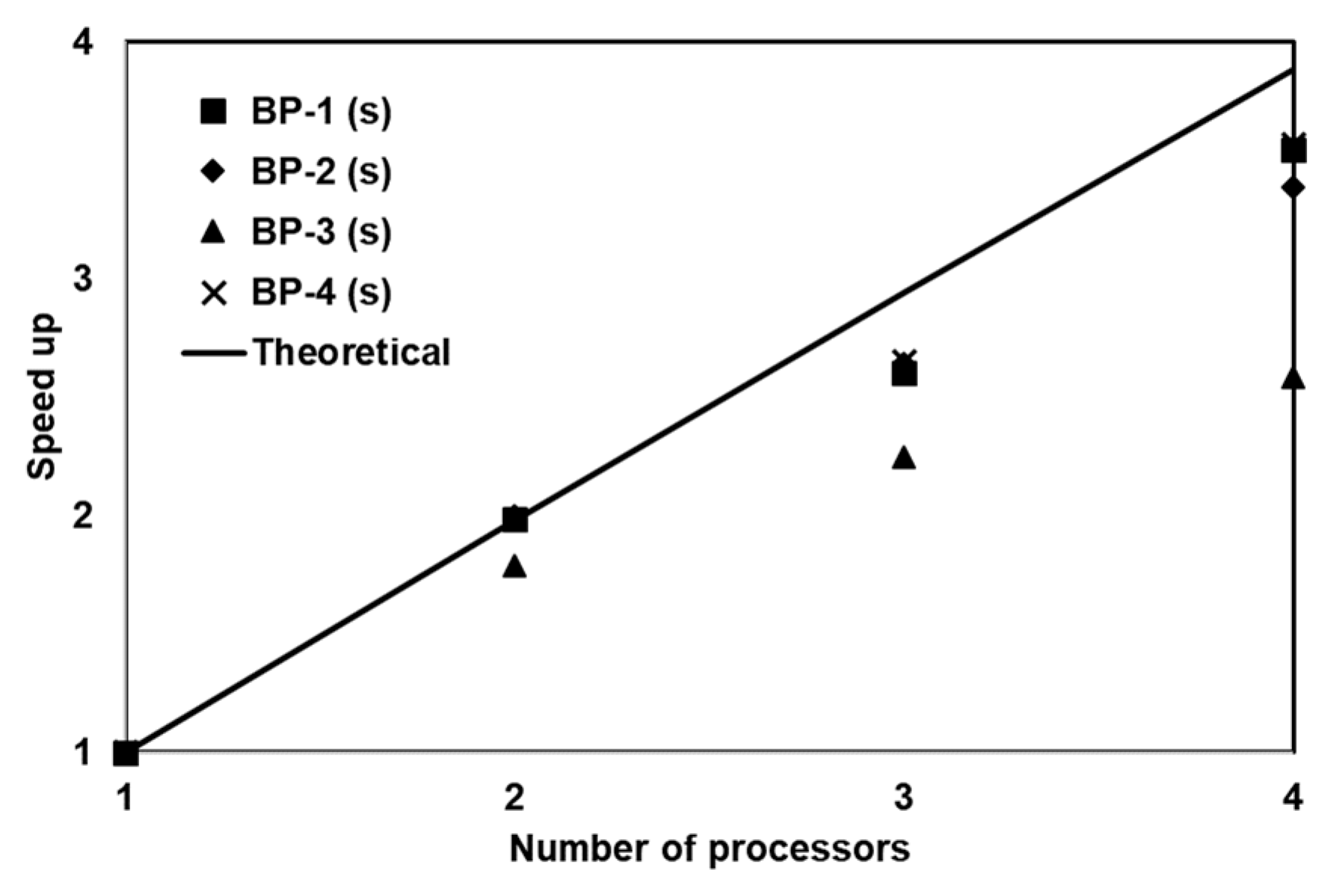
35] with the genetic algorithm for parameter estimation. The performance of the PGA was compared using four different benchmark problems and the speedup for the PGA using four threads on a desktop computer is also presented.

2. Materials and Methods

2.1. Genetic Algorithm Process

The six key steps involved in a traditional GA are encoding, population generation, selection, crossover, mutation, and termination [12]. The GA starts with a randomly generated initial set of solutions (also known as chromosomes) and this is called the initial population. The fitness of this population is calculated using the objective function. The fitness of each chromosome in the population is used to assess its ability to survive the current generation. For a minimization problem, a lower value of fitness is desirable. Based on this fitness value, two parents are chosen using a selection process. The selected parents undergo a crossover, where the genetic information is exchanged between the parents using a crossover function. Since the genetic information is transferred to the subsequent generation of children it is always preferable to choose individuals with better fitness in the selection process. It is also possible that an offspring generated from the crossover of the parents could undergo a mutation operation governed by a mutation probability. The fitness of the offspring is calculated and is combined with the entire population. Individuals with poor fitness are removed from the population (death) at the end of the generation. There are several strategies available for discarding bad solutions, and for implementing the process of encoding, selection, crossover, and mutation. The specific methods used in this study are discussed below.

2.2. Details of the Genetic Algorithm Used in this Study

In this study, a real value encoding is used because each parameter value in our problem could have different magnitudes. Studies have shown that engineering applications, which are sensitive to parameter variations, perform better with the real value encoding method than the binary encoding method [17,36,37]. We generated an initial population of 32 solutions within a specified range given by the user. The parameter values were then transformed to log (of base 10) scale and a uniform random number (distributed between 0 and 1) was used to generate various random parameter values using the formula: log (low) + r × [log (high) − log (low)], where r is the random number. These values were then raised to the power of 10 (to transform back to real number scale) and were used to populate the chromosome. We were not able to find a function that is able to generate a chromosome of different magnitudes using real value encoding in the literature. Therefore, this method was chosen arbitrarily to generate our initial population within the given bounds. We have used the FORTRAN version of RT1D to complete the reactive transport simulations and compute the final concentrations. The details of this one-dimensional model and the numerical methods used for advection, dispersion, and reaction are presented in Torlapati and Clement [35]. The concentrations generated from these initial parameters were used to calculate the sum square of errors (SSE) between model-predicted concentrations and those obtained from experimental data. This calculated SSE value was assigned as the fitness parameter for that chromosome. The selection of parents was done using a tournament selection method [38]. In this method, the algorithm randomly selected five possible candidates for the parents from the population and the individual with the best fitness is chosen as the parent. The process was repeated to find the second parent. Tournament selection allows the selection of individuals with the best fitness so that their genetic material can be passed on to the next generation [38]. The selected parents underwent a crossover using a weighted average. The weights between the parents are chosen by randomly generating a real number (r) between 1 and 0.5. If the chosen random number is r, then the new parameters are calculated by the formula: r × parent1 + (1 − r) × parent2 [25]. This weightage within the bounds of 1 and 0.5 allows us to keep the offspring within the boundaries specified at the beginning of the program. If the random number generated is close to 0.5, then we have an average of both the parents, whereas if the random number generated was close to the higher bound (of 1), then the value of the offspring will be closed to the first parent. A total of eight children were generated by performing the crossover eight times. The total number of children and the initial population were ensured to be multiples of four so that the total load distributed on each processor (we used four processors; details are given below) during parallelization is equal. These children could also undergo a mutation step if a randomly generated number is less than the probability of mutation (Pm). The mutation operator used in this algorithm multiplies the parameter by 0.5 before ensuring that it does not cross the bounds set at the beginning of the program. The fitness of the offspring is calculated and is combined with the initial population. The population is then sorted according to its fitness and the best 32 solutions are preserved for the next generation. The best solution is always preserved in this fashion and hence this algorithm can be classified as an elitist approach. The process of selection, crossover, mutation, and death was repeated for about 100 generations, and it was observed from our sensitivity analysis studies that the GA solution does not improve after about 100 generations.

2.3. Parallelization of the Genetic Algorithm

GA provides a natural and easy approach for parallelization within each generation since most of the loops within a generation contain variables that are not dependent on its value at the previous iteration. This allows for little to virtually no communication time between the processors for synchronization. The parallelization of the GA was achieved by using the shared memory programming procedure OpenMP available within the Intel FORTRAN90 compiler. The desktop computer (Dell, Round Rock, TX, US) used for performing simulations used an Intel Xeon quad-core processor, with a total of four processors available for parallelization.
The parallelization was accomplished by placing OpenMP constructs at the beginning and the end of the loop that is desired to be run in parallel mode. The OpenMP constructs are also used to specify the number of processors to be used for parallelization and the variables that are private or public to each processor and the kind of schedule to be used to distribute the load among the processors. A guided schedule was used in this study.
The loops that were parallelized include the fitness calculation of the initial population since this was the most time-consuming part of the program. Also, the fitness calculations of the offspring were completed in a parallel mode. Figure 1 illustrates the computational steps involved in implementing the PGA algorithm for a four-processor system. Although the selection, crossover, and mutation processes can be performed in parallel, these are not computationally intensive tasks; we found the performance gains to be marginal when these loops were optimized.

2.4. Details of the Numerical Model Used for Fitness Calculation

To calculate the fitness of the chromosomes, a multicomponent one-dimensional reactive transport model was used. The numerical model is a Fortran version of a previously published Visual Basic software RT1D [35]. The model solves a set of advection-dispersion-reaction equations that describe the transport of “m” mobile components and “n” immobile components. The general form of the transport equations is as follows [35]:
R i C i t = V C i x + D 2 C i x 2 + β i     where   i = 1 , 2 , 3 m
R j S j t = β j     where   j = ( m + 1 ) ,   ( m + 2 ) ,   ( m + 3 )   ( m + n )
where V is the velocity (m/day), D is the hydrodynamic dispersion coefficient (m2/day), Ci is the aqueous phase concentration (mg/L) of mobile component “i,” where i = 1, 2...m; Sj is the solid phase concentration (mg/mg) of immobile component “j,” where j = m + 1, m + 2... m + n; Ri and Rj are the linear retardation factor for the mobile and immobile components respectively; and βi & βj are the reaction terms for the mobile and immobile components, respectively. Note the immobile component equations do not have the advection-dispersion terms but will have a reaction term that might be coupled to other reaction terms in mobile components.
The Equation (1) and Equation (2) are numerically solved using the operator split strategy [35,39]. An implicit finite difference scheme was used to solve the advection-dispersion part of the equation and the reaction part, which reduces to a set of ordinary differential equations, is solved using a Runge–Kutta–Felhberg with adaptive time-stepping [40]. The model concentrations obtained for each chromosome were used to calculate the absolute error using the given experimental dataset. This error was squared and a sum of all these errors was calculated and was designated as the fitness for the chromosome. The objective of the PGA was to minimize this sum square of errors.

2.5. Details of the Benchmark Problems used for PGA Performance

In order to test the performance of the PGA, we have picked four different benchmark problems whose unknown parameters were published in the literature. PGA was used to reproduce these unknown parameters from the benchmark problems. Since coupled reactive transport problems have complex solution space, we have picked problems that have analytical solutions or published numerical solutions. Furthermore, the parameters predicted by the PGA can be used to predict the trends and compare them to the published trends. A brief summary of these problems is presented in Table 1.
Benchmark Problem 1 is a rate-limited sorption process model that shows the interaction between a mobile component and an immobile component. Toride et al. [5] presented analytical solutions for this type of interaction between mobile and immobile components. This analytical solution strategy was used by Valocchi and Werth [41] to develop a Java applet that can be run on a webpage.
Benchmark Problem 2 showcases the sequential decay of four different coupled mobile components with distinct retardation factors. Quezada et al. [42] presented analytical solutions using Laplace transformation and linear transformation to uncouple the coupled partial differential equations.
Benchmark Problem 3 involves the biodegradation of trichloroethene (TCE) into its subsequent compounds dichloroethenes (DCE), vinyl chloride (VC), and ethene in a batch reactor. The Monod kinetics model was used to model the growth of mobile and immobile bacteria in the presence of substrate. The experimental dataset was modeled using a trial and error process by Schaefer et al. (2009) [3].
Benchmark Problem 4 involves the biodegradation of carbon tetrachloride (CT) in the presence of denitrifying bacteria (KC), acetate, and nitrate. Phanikumar et al. [43] used the Sequential Quadratic Programming toolbox in MATLAB to find the unknown parameters. In order to reduce the number of unknown parameters, they used values from the literature for some parameters in their model. In addition, they were able to show the fitness of the objective function when the parameters deviated from an optimal value (Figure 2 in Phanikumar et al. [43]).
The specific kinetic equations used for modeling these benchmark problems and their unknown parameters are presented in the following section.

3. Results

To test the performance of the PGA, four different benchmark problems of varying complexity were selected. The benchmark problems chosen in this study have analytical solutions or published numerical solutions for unknown parameters. In addition, experimental data is also available for benchmark problems 3 and 4. Therefore, we have used the experimental data as input to obtain the unknown parameters. After completing the parameter identification step, we performed speedup tests by varying the number of threads and quantified the advantages of adding of parallelized algorithm vs. a sequential algorithm. In addition, sensitivity analysis studies were performed to identify the sensitivity of the solution to changes in the initial population size and the total number of generations.

3.1. Benchmark Problem 1: Parameter Estimation in a Rate-Limited Sorption Problem

In this benchmark problem, we solve a rate-limited sorption process where nonequilibrium conditions exist. Clement et al. [39] and Torlapati and Clement [35] modeled these kinetic processes using the following governing equations.
C t = V C x + D 2 C x 2 ξ ( C S K d )
dS dt = φ ξ ρ ( C S K d )
where C is the concentration in the component in the aqueous phase (mg/L), S is the concentration of the component in the solid phase (mg/mg), ρ is the bulk density (mg/L), φ is the porosity, Kd is the linear sorption constant (L/mg), k is the first-order decay constant (day−1), and ξ is the mass transfer coefficient (day−1).
The unknown parameters in this problem are D, ξ, and Kd. The model was run in the forward simulation model using known parameter values, and the aqueous phase concentrations predicted after 50 days was used as the data. The pore velocity used in this problem was 0.53 cm/day. The concentration values were made available at every 2 cm over a 30 cm long column. The temporal and spatial time steps used were 0.4 cm and 0.01 days, respectively. The lower and higher bounds for each unknown model parameters were perturbed by two orders of magnitude (one in each direction), as shown in Table 1. The parameters estimated by the PGA after 100 generations are given in Table 1 along with their published values. The minimum value of fitness obtained at the end of PGA simulations was 2.5 × 10⁻⁵. It can be seen from Table 1 that the parameter values estimated by the code are close to the original values. A comparison of the concentration profiles simulated using PGA-estimated parameter values and the published parameter values are shown in Figure 2. It can be seen from the figure that the PGA-estimated model predictions fit this synthetic dataset well. Table 2 also shows that the parameter values estimated by PGA have less than 5% error from the original estimates.

3.2. Benchmark Problem 2: Parameter Estimation in a Sequential Decay Problem

Quezada et al. [42] presented analytical solutions for solving coupled multidimensional multicomponent transport equations involving first-order kinetic interactions. This is a four-component problem with four kinetic parameters and a distinct retardation factor for each component. The governing transport equations are:
R 1 C 1 t = V C 1 x + D 2 C 1 x 2 k 1 C 1
R 2 C 2 t = V C 2 x + D 2 C 2 x 2 + F c 2 / c 1 Y c 2 / c 1 k 1 C 1 k 2 C 2 + F c 2 / c 3 Y c 2 / c 3 k 3 C 3
R 3 C 3 t = V C 3 x + D 2 C 3 x 2 + F c 3 / c 1 Y c 3 / c 1 k 1 C 1 + F c 3 / c 2 Y c 3 / c 2 k 2 C 2 k 3 C 3
R 4 C 4 t = V C 4 x + D 2 C 4 x 2 + F c 4 / c 2 Y c 4 / c 2 k 2 C 2 + F c 4 / c 3 Y c 4 / c 3 k 3 C 3 k 4 C 4
where Ci is the aqueous concentration of component i (i = 1, 2, 3 or 4) (mg/L), Ri is the linear retardation factor for the component i, ki is the first-order degradation constants for the component i (day−1), Y is the yield coefficient between two components, F is the fraction of yield between two components. The unknown parameters in this benchmark problem are: D, k1, k2, k3, and k4. The concentrations of all the components at an interval of 1 cm along the 30 cm long column predicted after 50 days of transport were made available for the fitness calculation. The pore velocity used in this problem was 0.4 cm/day. The time step and the grid size used for the simulations were 0.1 days and 0.1 cm, respectively. The yield values were set to 1. The simulation was run for 100 generations and the minimum SSE observed was about 1.5 × 10⁻². The comparison of the PGA-estimated parameters along with their low and high bounds used assumed in the simulation are given in Table 3. The concentration profiles generated using PGA-estimated parameters and the published parameters are shown in Figure 3. It can be observed from the figure that both solutions match well. The error in the parameter values varies from 4 to 38%.

3.3. Benchmark Problem 3: Parameter Estimation for a TCE Biodegradation Model

Schaefer et al., [3] conducted batch experiments to study the degradation of TCE in the presence of Dehalococcoides Sp. They used modified Monod kinetics to model the bioaugmentation process and the associated biochemical reactions. The kinetic equations are:
dC TCE dt = 1 R TCE [ q TCE XC TCE C TCE + K TCE ]
dC DCE dt = 1 R DCE [ q DCE XC DCE C DCE + K DCE ( 1 + C TCE I TCE ) ] + 1 R TCE [ q TCE XC TCE C TCE + K TCE ]
dC VC dt = 1 R VC [ q VC XC VC C VC + K VC ( 1 + C TCE I TCE + C DCE I DCE ) ] + 1 R DCE [ q DCE XC DCE C DCE + K DCE ( 1 + C TCE I TCE ) ]
dX dt = YX [ 1 R TCE q TCE C TCE C TCE + K TCE + 1 R DCE q DCE C DCE C DCE + K DCE ( 1 + C TCE I TCE ) + 1 R VC q VC C VC C VC + K VC ( 1 + C TCE I TCE + C DCE I DCE ) ]
where Ci (mM) and X (cells/L) are the concentration of ith compound and biomass, respectively; i can be either TCE, DCE, or VC; qi is the maximum biomass utilization rate (mmol/L/(cell h)), Ki is the half velocity coefficient of the compound (mM), I is the competition coefficient (mM), Ri is a retardation term that accounts for the presence of air in the system [3].
The unknown model parameters are: qTCE, qDCE, qVC, KTCE, KDCE, KVC, and IDCE as they were estimated by the authors of the original paper. The batch simulation experiments were performed for a total of 12 days and the time step used was about 0.01 days. The initial concentrations of TCE, ethene, and biomass were 0.08 mM, 0.003 mM, and 2.8 × 10¹⁰ cells/L, respectively. The biomass yield coefficient used in this problem was 4.4 × 10⁹. The concentrations of TCE, DCE, VC, and ethene obtained from the experimental data were provided for the calculation of the fitness of the PGA. The PGA was run for 100 generations and the PGA-estimated model parameters are compared with the “true values” and the corresponding relative errors are given in Table 3. The table also provides the lower and upper bounds used in this PGA search. The comparison of the concentration profiles with the experimental results with the published parameters as well as the PGA-estimated parameters are shown in Figure 4a,b respectively. The experimental results shown in the Figure are provided as the input for the PGA fitness calculations. It can be seen from Table 4 that some of the parameters have relatively high error percentages (200–400%) when compared to the published values. It should be noted that the authors in the paper used a trial-and-error process to obtain the kinetic parameter values. In order to compare the errors between the published and PGA-estimated parameters, we compared the sum square of errors (fitness) for the simulated results from both cases. The sum square of errors for the published parameters and the PGA-estimated parameters were 0.0021 and 0.0018. Therefore, the results from the PGA-estimated parameters were marginally better than the published results and explained the relatively high error percentage compared to the published parameters.

3.4. Benchmark Problem 4: Parameter Estimation for a Carbon Tetrachloride Bioremediation Problem

Phanikumar et al. [43] conducted experiments to study the bioremediation of carbon tetrachloride (CT) contaminated column which was intermittently fed with nutrients such as acetate and nitrate. They developed a reactive transport model for the system and used a modified version of the RT3D code to simulate their experimental data. The model included a total of four mobile and two immobile components. The mobile components in the system were CT, acetate, nitrate, and the mobile bacteria, whereas the immobile components were the sorbed CT and immobile phase bacteria. The kinetic reaction equations used in the reactive transport model are:
( 1 + ρ fK d θ ) dC CT dt = k C CT ( X M + X IM ) ρ κ θ [ ( 1 f ) K d C CT S CT ]
R a dC a dt = μ max M a M n Y a ( X M + X IM )
R n dC n dt = μ max M a M n Y n ( X M + X IM ) [ b KC Y nb ( 1 M a ) + γ M n ] ( X M + X IM )
dX M dt = [ μ max M a M n b KC ( 1 M a ) K at ] X M + K de ( 1 M a ) X IM
dS CT dt = κ [ ( 1 f ) K d C CT S CT ]
dX IM dt = [ μ max M a M n b KC ( 1 M a ) K de ( 1 M a ) ] X IM + K at X M
where f is the fraction of equilibrium sites, bKC is the microbial decay rate (day−1), Kat is the attachment coefficient (day−1), Kde is the detachment coefficient (day−1), k’ is the CT reaction rate (day−1), γ is the nitrate reaction rate (day−1), κ is the kinetic desorption rate (day−1), µmax is the maximum specific growth rate (day−1), Ya, Yn and Ynb are the yield rates of acetate, nitrate, and biomass, respectively; CCT, Ca, Cn, and SCT are the aqueous concentrations of carbon tetrachloride, acetate, nitrate, and the sorbed concentration of carbon tetrachloride, respectively; XM and XIM are the concentrations of mobile and immobile bacteria, respectively. Also, Ma and Mn are the Monod terms for acetate and nitrate reactions, respectively, and given by the expressions: M a = C a K sa + C a and M n = C n K sn + C n where Ksa and Ksn are the half-saturation coefficients of acetate and nitrate utilization reactions, respectively. Further details of the model and the experiment are given in Phanikumar et al., [43] and Torlapati and Clement [35].
The unknown parameters in this model are: k’, γ, Kde, and bKC as it was done in the published paper. The known parameters for this model are summarized in Table 5. The known concentrations values after 4 days of operation at each node point were supplied to the PGA to calculate the fitness. The PGA was run for 100 generations and the SSE after 100 generations was 666. The fitness value was higher in this case due to the magnitude of the acetate. The PGA-estimated parameters are compared against the published values in Table 6; the table also provides estimated error for each parameter value and the lower and higher bounds values. The concentration profiles predicted by the PGA-estimated parameters and compared against the simulated data points from published parameters are presented in Figure 5a–d. It can be observed from the figure that the results compare well.

3.5. Understanding the Scalability of the Parallel GA

The computational performance of the PGA was tested on a quad-core Intel computer. All four benchmark problems were run using either 1, 2, 3, or all 4 processors and the total run time was calculated using the omp_wall_time() function. This internal clock time function was called at the beginning of the program and subsequently at the end of the program. The difference between these two times gave an estimate of total program runtime. The observed speedup of the parallel program was calculated using the formula:
o b s e r v e d   s p e e d u p p a r a l l e l = sequential   time parallel   time
The sequential time in Equation (19) was obtained by solving the problems using a single processor. The theoretical speedup of the algorithm was calculated using Amdahl’s law, given below [44].
t h e o r e t i c a l   s p e e d u p p a r a l l e l = 1 ( 1 f ) + f n
where f is the fraction of the program that is parallelized, and n is the number of processors. For the PGA, we have used an f value of 0.99 since the most computationally intensive parts of the algorithm are fitness calculations. These fitness calculations are done in parallel as shown in Figure 1. The observed speedup of the PGA for different benchmark problems and its comparison against the theoretical speed calculated by Amdahl’s law for four threads are shown in Figure 6. The simulation times for all benchmark problems for the different number of threads are summarized in Table 7. It can be observed from the figure that the performance of the PGA for all the benchmark problems is close to the ideal linear speedup function, except for the third benchmark problem. This is because the total simulation time taken for Problem 3 was extremely small and hence the calculation of fitness was not as computationally intensive compared to other benchmark problems. In a problem where the parallelized parts of the problem are not as computationally intensive, the time taken to perform the nonparallelized tasks becomes a limiting factor and thereby reduces the total efficiency of the parallel operations.

3.6. Sensitivity of PGA to Initial Population and Generations

The final quality of the solution that is found by the PGA depends on the size of the initial population generated and the number of generations. Ideally, a larger number of initial solutions would allow the PGA to search through a larger solution space, but this also increases the computational burden as the fitness must be calculated for all the initial solutions. On the other hand, having a smaller initial population would limit the solution space of the PGA and this could cause the PGA to be trapped in a local minimum. To check the sensitivity of PGA to the size of the initial population and the number of generations, we ran all four benchmark problems using four different initial population sizes; 8, 16, 32 and 64. In addition, we increased the total number of generations to 300. The best solution for each generation was stored to compare the general convergence pattern for different initial population sizes. The results from the sensitivity analysis for all four benchmark problems are shown in Figure 7a–d. It can be observed from the results that the convergence rate was faster when the initial population size was increased; however, increasing the number of generations did not affect the quality of the solution found by the algorithm. Also, in the case of simulations with smaller population sizes, the minimum value reached was away from the global minimum value. It is necessary to find an optimal initial population size, and this could vary based on the number of parameters being estimated. Increasing the population size might not always result in a better solution as an increase in population size from 32 to 64 did not improve in the solutions. For problems involving high levels of computational complexity, the evaluation of another 32 candidates for fitness could increase the overall simulation time drastically without improving the solution. In this study, we found a population size of 32 to be the optimal number in all our simulations.

3.7. Sensitivity to Parameter Bounds

The rate of convergence and the quality of the final solution is also a function of the level of uncertainty (characterized by bounds used to define the minimum and maximum values) associated with the unknown parameter. To understand the sensitivity of PGA to these bounds, we ran test Problem 1 for different scenarios using different bounds. This problem was selected because some parameters in this problem were highly sensitive, and even a minor change would cause considerable fluctuations in the concentration profiles. We developed four different scenarios to test the sensitivity of PGA to parameter bounds. In the first scenario, the bounds were kept within an order of magnitude of the true parameter; in the second scenario, the lower bound was reduced by an order of magnitude; in the third scenario, the lower bound is kept the same as the first scenario, but the higher bound was increased by an order of magnitude, and in the fourth scenario both lower and higher bounds were changed by an order of magnitude. Therefore, in scenarios 2 and 3, the order of magnitude difference between the lower and higher bounds was two and in the case of scenario 4, the difference is three. Table 8 summarizes the lower and higher bounds used in all four scenarios. The concentration profiles predicted under different scenarios are shown in Figure 8. It can be observed from the Figure that the quality of the solution deteriorated as the bounds for the unknown parameters were increased above one order of magnitude and it was particularly worse for scenario 4. This shows that the PGA requires reasonable constraints (within one order of magnitude) for the unknown parameters with high level of uncertainty. In most cases, the values published in literature can be used as reasonable initial constraints. If this information was unavailable, then PGA can be run multiple times by refining the bounds until the fitness of the objective function is reasonable.
The PGA used in this study works by systematically searching through a given solution space to find the best solution. Therefore, when the unknown parameters have a high degree of uncertainty, it would be helpful to constrain the problem within an order of magnitude. The quality of the initial population is largely dependent on the bounds set by the user at the beginning of the simulation. Reactive transport problems could contain highly sensitive parameters that could significantly alter the solution even with the changes are small. Therefore, depending on the type of problem, the user might have to restrict some unknown parameters within the PGA to a narrow boundary, if the solution has convergence problems.

4. Summary and Conclusions

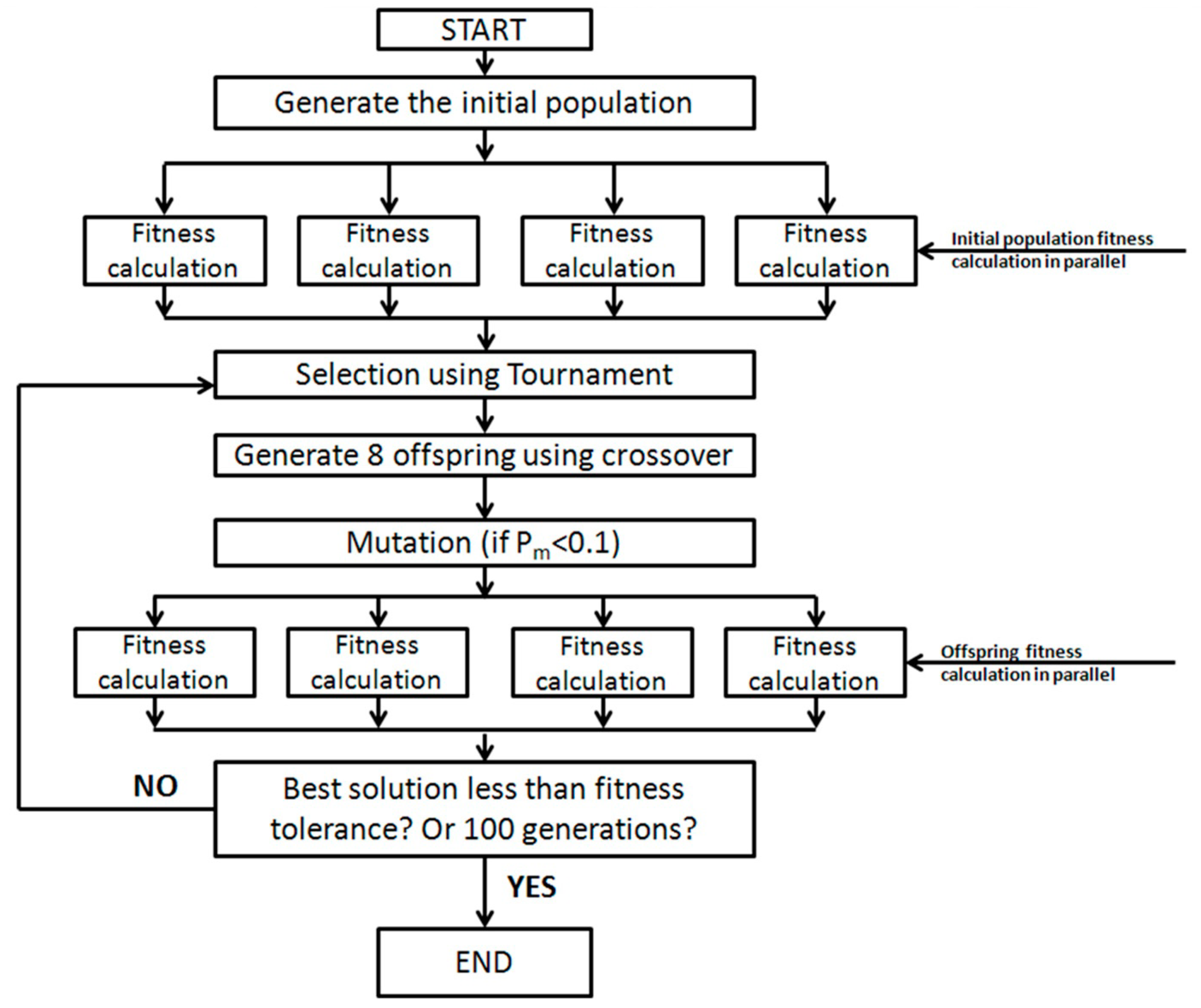
In this study, we coupled a PGA with a one-dimensional multicomponent reactive transport model, RT1D, to develop a parameter estimation tool. PGA can directly use the existing forward model with randomly generated initial population to converge to the best fit parameter. The presence of randomness in the initial population and their ability to preserve the best solutions enables them to search through a vast population to find the global minimum. In addition, the algorithm can also be parallelized since the fitness calculations can be performed simultaneously on separate processors. This allows for a significant reduction in program runtime where the fitness calculations are computationally intensive.
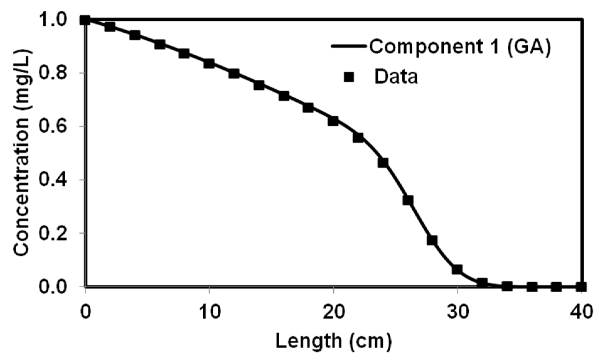
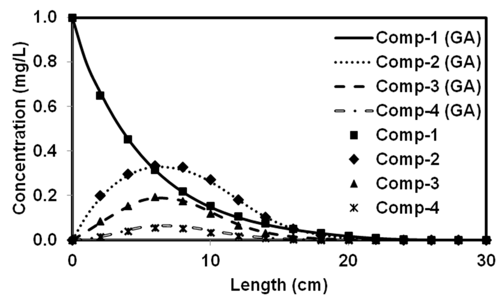
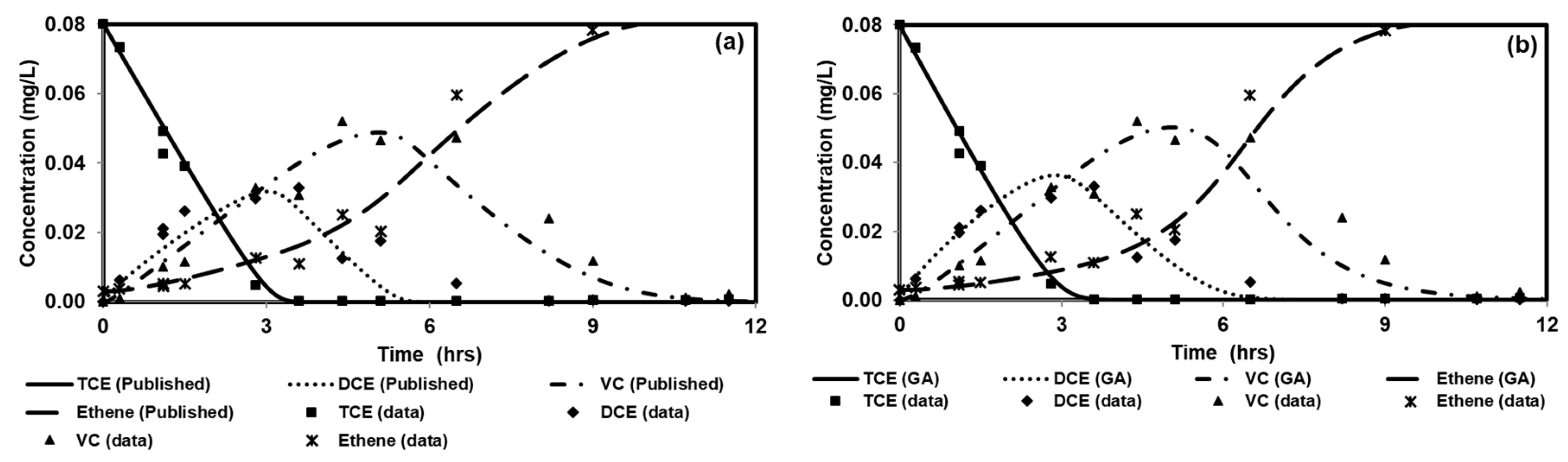
We tested the performance of a parallel version of PGA by solving four benchmark problems that simulated both batch and reactive-transport scenarios. The benchmark problems chosen to test the performance of the algorithm have analytical solutions and published numerical solutions. The PGA algorithm was able to reproduce the model parameters with minimum error for both analytical benchmark problems. Furthermore, the simulation results from these parameters were able to match the original experimental or analytical/numerical data well. For benchmark problems 3 and 4, the PGA was provided with the experimental data as the input and we were able to fit the data well in both cases. Particularly, for benchmark problem 3 where the trial-and-error method was used, we were able to show better fitness than the original model. The PGA presented in this study was versatile and did not require any problem-specific modifications except for the kinetic equations which were solved by the one-dimensional reactive transport model, RT1D.
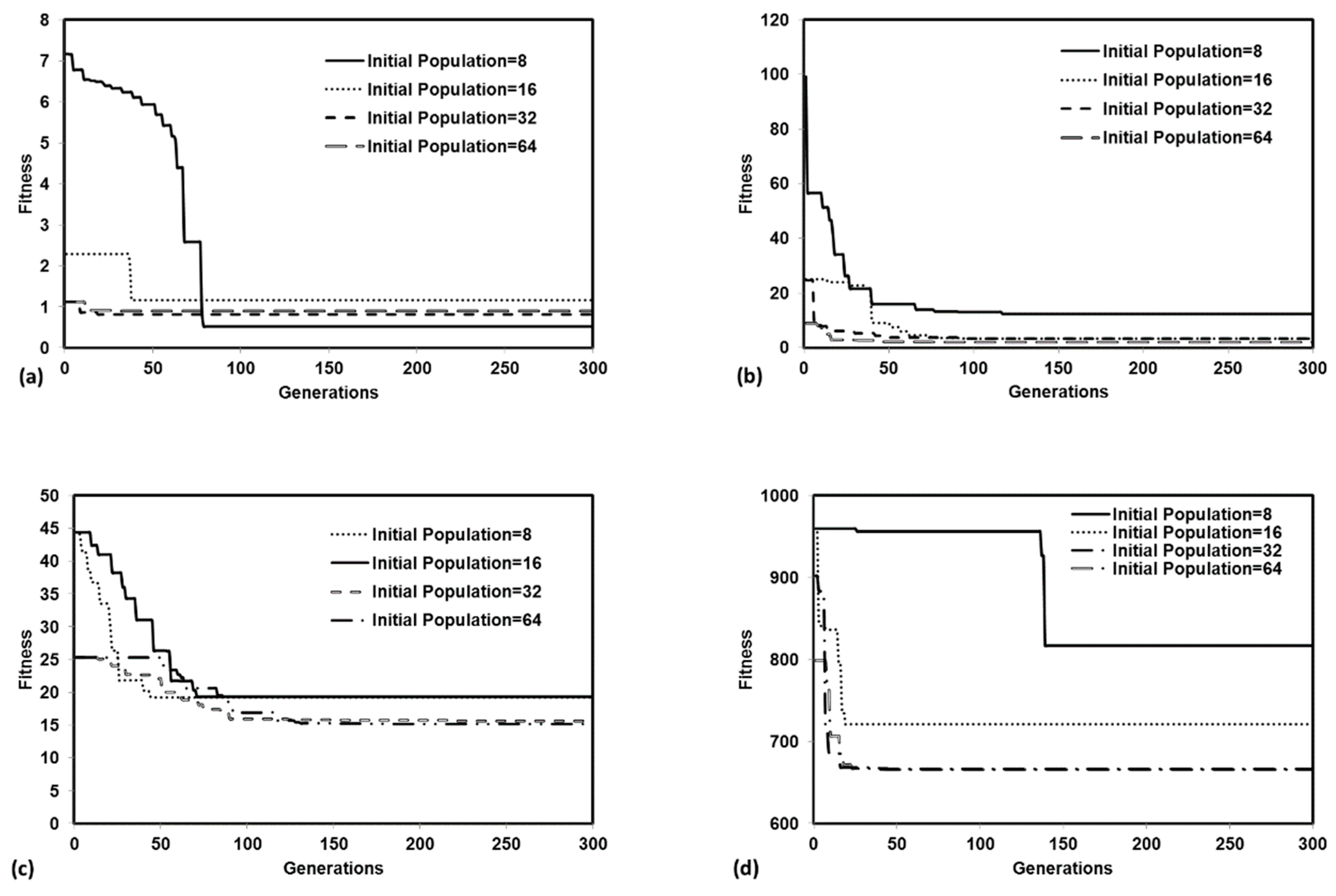
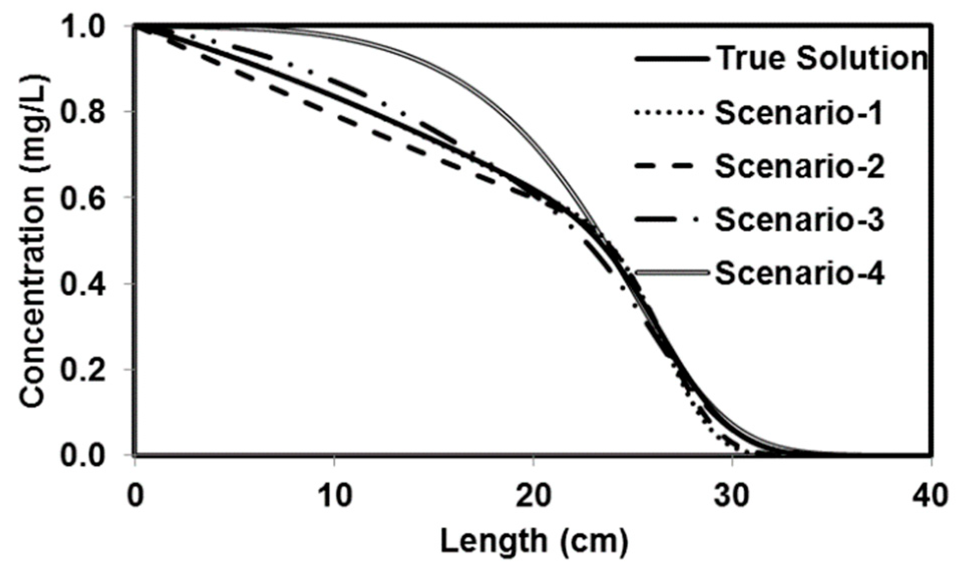
Sensitivity studies show that our model is sensitive to the initial bounds for each parameter when the difference in the order of magnitudes for the lower and higher bounds was too large. For the benchmark problems tested in the study, the lower and higher bounds were at least one order of magnitude higher. The observed trends in the sensitivity studies were still within the margin of error for two orders of magnitude but were particularly worse when the difference in the order of magnitudes was three times (scenario 4). In most real cases, the user should have access to the order of magnitude for the unknown parameters from the literature. This could potentially be a limitation if the unknown parameter does not have published values. However, the model can be calibrated by starting with a larger bound and can be refined with multiple iterations. The user should, however, be careful not to overconstrain the problem and ensure that the upper and lower parameter bounds are adequately large to generate enough initial solutions to avoid convergence to a local optimum. Parameter estimation techniques are used to minimize the objective function and present solutions. Doherty and Hunt [6] discuss the importance of user expertise in determining the feasibility of solutions as well as constraining the optimization problem. If more parameters are estimated than the valid dimension, it is possible that we increase the number of feasible solutions. The uncertainty of parameters in groundwater reactive transport problems is further discussed in Shi et al. [9].
The PGA was optimized to run in the parallel mode using the OpenMP framework available within the Intel FORTRAN v9.0 compiler on a shared memory system. The speedup was quantified for four benchmark problems and the results indicate close to linear speedup for three benchmark problems. The fourth benchmark (designated as Problem 3) was a much simpler problem that required very little computational effort and hence the parallel computing steps did not reduce the overall computational time. These results show that the use of PGA was more appropriate for solving computationally intensive reactive transport problems. The overall computational gain obtained using this hardware was significant. Since most modern desktop PCs are now equipped with multicore processors, the methods used in this study can be easily adapted to take advantage of these platforms. The proposed optimization framework, which was used for estimating unknown kinetic and transport parameters in our multicomponent reactive transport problems, is a generic procedure that can be adapted to solve a variety of water quality problems. In addition, these benchmark problems can be used by other researchers to compare their optimization algorithms.

Author Contributions

Conceptualization, J.T. and T.P.C.; methodology, J.T.; software, J.T.; validation, J.T. and T.P.C.; formal analysis, J.T.; investigation, J.T.; resources, T.P.C.; data curation, J.T.; writing—original draft preparation, J.T.; writing—review and editing, J.T. and T.P.C; visualization, J.T.; supervision, T.P.C.; project administration, T.P.C.; funding acquisition, T.P.C.

Conflicts of Interest

The authors declare no conflict of interest.

References

  1. Engesgaard, P.; Kipp, K.L. A geochemical transport model for redox-controlled movement of mineral fronts in groundwater flow systems: A case of nitrate removal by oxidation of pyrite. Water Resour. Res. 1992, 28, 2829–2843. [Google Scholar] [CrossRef]
  2. Gramling, C.M.; Harvey, C.F.; Meigs, L.C. Reactive transport in porous media: A comparison of model prediction with laboratory visualization. Environ. Sci. Technol. 2002, 36, 2508–2514. [Google Scholar] [CrossRef] [PubMed]
  3. Schaefer, C.E.; Condee, C.W.; Vainberg, S.; Steffan, R.J. Bioaugmentation for chlorinated ethenes using Dehalococcoides sp.: Comparison between batch and column experiments. Chemosphere 2009, 75, 141–148. [Google Scholar] [CrossRef] [PubMed]
  4. Torlapati, J.; Clement, T.P.; Schaefer, C.E.; Lee, K.-K. Modeling Dehalococcoides sp. Augmented Bioremediation in a Single Fracture System. Ground Water Monit. Remediat. 2012, 32, 75–83. [Google Scholar] [CrossRef]
  5. Toride, N.; Leij, F.J.; Genuchten, M.T. The CXTFIT Code for Estimating Transport Parameters from Laboratory or Field Tracer Experiments (Ver 2.1); US Salinity Laboratory, Agricultural Research Service, US Department of Agriculture: Riverside, CA, USA, 1995.
  6. Doherty, J.E.; Hunt, R.J. Approaches to Highly Parameterized Inversion: A Guide to Using PEST for Groundwater-Model Calibration; US Department of the Interior, US Geological Survey: Reston, VA, USA, 2010.
  7. Baginska, B.; Milne-Home, W.; Cornish, P. Modelling nutrient transport in Currency Creek, NSW with AnnAGNPS and PEST. Environ. Model. Softw. 2003, 18, 801–808. [Google Scholar] [CrossRef]
  8. Yabusaki, S.B.; Fang, Y.; Long, P.E.; Resch, C.T.; Peacock, A.D.; Komlos, J.; Jaffe, P.R.; Morrison, S.J.; Dayvault, R.D.; White, D.C. Uranium removal from groundwater via in situ biostimulation: Field-scale modeling of transport and biological processes. J. Contam. Hydrol. 2007, 93, 216–235. [Google Scholar] [CrossRef] [PubMed]
  9. Shi, X.; Ye, M.; Curtis, G.P.; Miller, G.L.; Meyer, P.D.; Kohler, M.; Yabusaki, S.; Wu, J. Assessment of parametric uncertainty for groundwater reactive transport modeling. Water Resour. Res. 2014, 50, 4416–4439. [Google Scholar] [CrossRef]
  10. Massoudieh, A.; Mathew, A.; Ginn, T.R. Column and batch reactive transport experiment parameter estimation using a genetic algorithm. Comput. Geosci. 2008, 34, 24–34. [Google Scholar] [CrossRef]
  11. Majdalani, S.; Fahs, M.; Carrayrou, J.; Ackerer, P. Reactive transport parameter estimation: Genetic algorithm vs. Monte carlo approach. Am. Inst. Chem. Eng. 2009, 55, 1959–1968. [Google Scholar] [CrossRef]
  12. Holland, J.H. Adaptation in Natural and Artificial Systems; University of Michigan Press: Ann Arbor, MI, USA, 1975. [Google Scholar]
  13. El Harrouni, K.; Ouazar, D.; Walters, G.A.; Cheng, A.H.D. Groundwater optimization and parameter estimation by genetic algorithm and dual reciprocity boundary element method. Eng. Anal. Bound. Elem. 1996, 18, 287–296. [Google Scholar] [CrossRef]
  14. Wang, Q. Using genetic algorithms to optimise model parameters. Environ. Model. Softw. 1997, 12, 27–34. [Google Scholar] [CrossRef]
  15. Wang, M.; Zheng, C. Optimal remediation policy selection under general conditions. Ground Water 1997, 35, 757–764. [Google Scholar] [CrossRef]
  16. Mulligan, A.E.; Brown, L.C. Genetic algorithms for calibrating water quality models. J. Environ. Eng. 1998, 124, 202–211. [Google Scholar] [CrossRef]
  17. Reed, P.; Minsker, B.; Goldberg, D.E. Designing a competent simple genetic algorithm for search and optimization. Water Resour. Res. 2000, 36, 3757–3761. [Google Scholar] [CrossRef] [Green Version]
  18. Giacobbo, F.; Marseguerra, M.; Zio, E. Solving the inverse problem of parameter estimation by genetic algorithms: The case of a groundwater contaminant transport model. Ann. Nucl. Energy 2002, 29, 967–981. [Google Scholar] [CrossRef]
  19. Singh, A.; Minsker, B.; Takagi, H. Interactive Genetic Algorithms for Inverse Groundwater Modeling: Issues with Human Fatigue and Prediction Models. In Impacts of Global Climate Change, Proceedings of the World Water and Environmental Resources Congress 2005, Anchorage, AK, USA, 15–19 May 2005; American Society of Civil Engineers: Reston, VA, USA, 2005. [Google Scholar] [Green Version]
  20. Béranger, S.C.; Sleep, B.E.; Lollar, B.S.; Monteagudo, F.P. Transport, biodegradation and isotopic fractionation of chlorinated ethenes: Modeling and parameter estimation methods. Adv. Water Resour. 2005, 28, 87–98. [Google Scholar] [CrossRef]
  21. Singh, A.; Minsker, B.S.; Valocchi, A.J. An interactive multiobjective optimization framework for groundwater inverse modeling. Adv. Water Resour. 2008, 31, 1269–1283. [Google Scholar] [CrossRef]
  22. Lee, S.; Heber, A.J. Ethylene removal using biotrickling filters: Part II. Parameter estimation and mathematical simulation. Chem. Eng. J. 2010, 158, 89–99. [Google Scholar] [CrossRef]
  23. Madsen, K.M.; Perry, A.E. Using Genetic Algorithms on Groundwater Modeling Problems in a Consulting Setting. In Proceedings of the Annual International Conference on Soils, Sediments, Water and Energy, Amherst, MA, USA, 18–21 October 2010; p. 11. [Google Scholar]
  24. Kontos, Y.; Katsifarakis, K. Optimization of management of polluted fractured aquifers using genetic algorithms. Eur. Water 2012, 40, 31–42. [Google Scholar]
  25. Cantú-Paz, E. A survey of parallel genetic algorithms. Calc. Paralleles Reseaux Syst. Repartis 1998, 10, 141–171. [Google Scholar]
  26. Abramson, D.; Mills, G.; Perkins, S. Parallelisation of a genetic algorithm for the computation of efficient train schedules. Parallel Comput. Transput. 1994, 37, 139–149. [Google Scholar]
  27. Baluja, S. A Massively Distributed Parallel Genetic Algorithm; DTIC Document; School of Computer Science, Carnegie Mellon University: Pittsburgh, PA, USA, 1992. [Google Scholar]
  28. Fogarty, T.; Huang, R. Implementing the genetic algorithm on transputer based parallel processing systems. In Proceedings of the International Conference on Parallel Problem Solving from Nature, Dortmund, Germany, 1–3 October 1990; Springer: Berlin/Heidelberg, Germany, 1990; pp. 145–149. [Google Scholar]
  29. Tanese, R. Distributed genetic algorithms for function optimization. In Proceedings of the Third International Conference on Genetic Algorithms and their Applications, San Mateo, CA, USA, 1 December 1989; pp. 434–439. [Google Scholar]
  30. McKinney, D.C.; Lin, M.D. Genetic algorithm solution of groundwater management models. Water Resour. Res. 1994, 30, 1897–1906. [Google Scholar] [CrossRef]
  31. Tsai, F.T.C.; Katiyar, V.; Toy, D.; Goff, R.A. Conjunctive management of large-scale pressurized water distribution and groundwater systems in semi-arid area with parallel genetic algorithm. Water Resour. Manag. 2009, 23, 1497–1517. [Google Scholar] [CrossRef]
  32. Abramson, D.; Abela, J. A Parallel Genetic Algorithm for Solving the School Timetabling Problem; Division of Information Technology, CSIRO: Canberra, Australia, 1991. [Google Scholar]
  33. Sarma, K.C.; Adeli, H. Bilevel parallel genetic algorithms for optimization of large steel structures. Comput. Aided Civ. Infrastruct. Eng. 2002, 16, 295–304. [Google Scholar] [CrossRef]
  34. Fredrickson, N.R.; Afsahi, A.; Qian, Y. Performance characteristics of OpenMP constructs, and application benchmarks on a large symmetric multiprocessor. In Proceedings of the 17th Annual International Conference on Supercomputing, San Francisco, CA, USA, 23–26 June 2003; pp. 140–149. [Google Scholar]
  35. Torlapati, J.; Clement, T.P. Benchmarking a Visual-Basic based MultiComponent One-Dimensional Reactive Transport Modeling Tool. Comput. Geosci. 2012, 50, 72–83. [Google Scholar] [CrossRef]
  36. Gaffney, J.; Pearce, C.; Green, D. Binary versus real coding for genetic algorithms: A false dichotomy? ANZIAM J. 2010, 51, C347–C359. [Google Scholar] [CrossRef]
  37. Michalewicz, Z. Genetic Algorithms + Data Structures = Evolution Programs, 3rd ed.; Springer: New York, NY, USA, 1996. [Google Scholar]
  38. Koza, J. Genetic Programming; MIT Press: Cambrige, MA, USA, 1992. [Google Scholar]
  39. Clement, T.P.; Sun, Y.; Hooker, B.S.; Petersen, J.N. Modeling multispecies reactive transport in ground water. Ground Water Monit. Remediat. 1998, 18, 79–92. [Google Scholar] [CrossRef]
  40. Chapra, S.C.; Canale, R.P. Numerical Methods for Engineers with Programming and Software Applications, 3rd ed.; WCB/McGraw-Hill: Boston, MA, USA, 1998. [Google Scholar]
  41. Valocchi, A.J.; Werth, C.J. Web-based interactive simulation of groundwater pollutant fate and transport. Comput. Appl. Eng. Educ. 2004, 12, 75–83. [Google Scholar] [CrossRef]
  42. Quezada, C.R.; Clement, T.P.; Lee, K.K. Generalized solution to multidimensional multispecies transport equations coupled with a first-order reaction network involving distinct retardation factors. Adv. Water Resour. 2004, 27, 507–520. [Google Scholar] [CrossRef]
  43. Phanikumar, M.S.; Hyndman, D.W.; Wiggert, D.C.; Dybas, M.J.; Witt, M.E.; Criddle, C.S. Simulation of microbial transport and carbon tetrachloride biodegradation in intermittently-fed aquifer columns. Water Resour. Res. 2002, 38, 1–13. [Google Scholar] [CrossRef]
  44. Hill, M.D.; Marty, M.R. Amdahl’s law in the multicore era. Computer 2008, 41, 33–38. [Google Scholar] [CrossRef]
Figure 1. Illustration showing the flow of a parallel genetic algorithm (PGA).
Processes 07 00640 g001
Figure 2. Comparison of results from PGA-estimated parameters and the published parameters for benchmark problem-1.
Processes 07 00640 g002
Figure 3. Comparison of results from PGA-estimated parameters and the published parameters for benchmark problem 2.
Processes 07 00640 g003
Figure 4. Comparison of experimental results with (a) published parameters, (b) PGA-estimated parameters for benchmark problem 3.
Processes 07 00640 g004
Figure 5. Comparison of results from PGA-estimated parameters and the published parameters for benchmark problem-4 showing different components (a) Carbon tetrachloride CT, (b) acetate, (c) nitrate, and (d) mobile bacteria.
Processes 07 00640 g005
Figure 6. Speedup for all benchmark problems for different number of processors.
Processes 07 00640 g006
Figure 7. Change in best fitness at the end of each generation for different initial population sizes (8, 16, 32, 64) for (a) Benchmark problem 1, (b) Benchmark problem 2, (c) Benchmark problem 3, and (d) Benchmark problem 4.
Processes 07 00640 g007
Figure 8. Comparison of different scenarios of the high and low bounds with the true solution for benchmark problem 1.
Processes 07 00640 g008
Table 1. Summary of the benchmark problems used for testing the performance of PGA along with their solution strategy employed and their source.
Benchmark ProblemSolution StrategySource
1Rate-limited sorptionAnalytical SolutionValocchi and Werth (2004) [41]
2Sequential decayAnalytical SolutionQuezada et al. (2002) [42]
3TCE biodegradationTrial and ErrorSchaefer et al. (2009) [3]
4CT biodegradationSQPaToolbox in MATLABPhanikumar et al. (2002) [43]
a Note: SQP stands for Sequential Quadratic Programming toolbox present in MATLAB.
Table 2. Comparison of the PGA-estimated parameters with published values along with their bounds and percentage error for benchmark problem-1.
ParameterPublished ValueLower BoundHigher BoundGA EstimateError %
Longitudinal dispersion coefficient, D (cm2/day)8.00 × 10−21.00 × 10−21.00 × 10−17.80 × 10−22.50%
Mass transfer coefficient, ξ1.50 × 10−21.00 × 10−21.00 × 10−11.43 × 10−24.67%
Linear sorption constant, Kd (L/mg)1.84 × 10−41.00 × 10−41.00 × 10−31.90 × 10−43.26%
Table 3. Comparison of the PGA-estimated parameters with true solutions along with their bounds for benchmark problem 2.
ParameterPublished ValueLower BoundHigher BoundGA EstimateError %
Longitudinal dispersion coefficient, D (cm2/day)8.00 × 10−21.0 × 10−31.0 × 10−18.40 × 10−25.00%
Decay constant for Component 1, k1 (day−1)7.50 × 10−21.0 × 10−31.0 × 10−17.80 × 10−24.00%
Decay constant for Component 2, k2 (day−1)5.00 × 10−21.0 × 10−31.0 × 10−15.80 × 10−216.00%
Decay constant for Component 3, k3 (day−1)2.00 × 10−21.0 × 10−31.0 × 10−12.77 × 10−238.50%
Decay constant for Component 4, k4 (day−1)4.50 × 10−21.0 × 10−31.0 × 10−14.00 × 10−211.11%
Table 4. Comparison of the PGA-estimated parameters with true solutions along with their bounds for benchmark problem-3.
ParameterPublished ValueLower BoundHigher BoundGA EstimateError %
Biomass utilization rate for TCE, qTCE (mmol/L/cells h)3.2 × 10−31 × 10−41 × 10−25.47 × 10−370.94%
Biomass utilization rate for DCE, qDCE (mmol/L/cells h)2.0 × 10−31 × 10−41 × 10−26.12× 10−3206.00%
Biomass utilization rate for VC, qVC (mmol/L/cells h)1.4 × 10−21 × 10−31 × 10−17.10 × 10−2407.14%
Half velocity constant for TCE, KTCE (mM)1.3 × 10−121 × 10−131 × 10−111.42 × 10−129.23%
Half velocity constant for DCE, KDCE (mM)7.0 × 10−131 × 10−141 × 10−127.46 × 10−136.57%
Half velocity constant for VC, KVC (mM)1.4 × 10−121 × 10−131 × 10−115.10 × 10−12264.29%
Competition coefficient for DCE, IDCE (mM)5.2 × 10−31 × 10−41 × 10−24.20 × 10−319.23%
Table 5. Model parameters used for benchmark problem 4.
ParameterValue
Pore Velocity (cm/day)10
Length (cm)200
Longitudinal dispersion coefficient (cm2/day) (D)2
Δx (cm)1
Δt (days)0.001
Porosity (φ)0.35
Bulk density (ρ) (mg/L)1.63 × 106
Time (days)4
Fraction of equilibrium sites (f) 0.437
Attachment coefficient (day−1) (Kat) 0.9
Distribution coefficient (Kd) (L/mg)3.9 × 10−7
Half saturation coefficient: (mg/L)
Acetate (Ksa)1.0
Nitrate (Ksn)12.0
Kinetic desorption rate (day−1) (κ)0.36
Maximum specific growth rate (day−1) (μmax)3.11
Yield:
Acetate (Ya)0.4
Nitrate (Yn)0.25
Biomass (Ynb)0.46
Initial condition (ppm):
Carbon tetrachloride (CCT)0.130
Acetate (Ca)0
Nitrate (Cn)42
Mobile bacteria (XM)0
Immobile bacteria (XIM)0
Sorbed CT (mg/mg) (SCT)2.8 × 10⁻⁸
Boundary condition (ppm):
Carbon tetrachloride (CCT)0.130
Acetate (Ca)0
Nitrate (Cn)42
Mobile bacteria (XM)0
Immobile bacteria (XIM)0
Slug injection zone inoculation (ppm):
Carbon tetrachloride (CCT)0.1
Acetate (Ca)1650
Nitrate (Cn)42
Mobile bacteria (XM)11.8
Immobile bacteria (XIM)0
Note: Carbon tetrachloride is abbreviated as CT.
Table 6. Comparison of the PGA-estimated parameters with published parameters along with their bounds for benchmark problem 4.
ParameterPublished ValueLower BoundHigher BoundGA EstimateError %
CT reaction rate (day−1) (k’)0.1890.10.50.28249.21%
Nitrate utilization coefficient (day−1) (γ)5.731105.892.79%
Detachment coefficient (day−1) (Kde)0.0430.010.10.06346.51%
Microbial decay rate (day−1)(bKC)0.2210.110.2190.90%
Table 7. Simulation times for all the benchmark problems for different number of processors in seconds.
# ProcessorsBP-1 (s)BP-2 (s)BP-3 (s)BP-4 (s)
1885.00132.007.003920.00
2446.0066.003.921976.00
3339.7350.003.121479.00
4249.6339.002.711100.00
Note: BP—benchmark problem.
Table 8. High and low bounds for the four different scenarios along with the PGA-estimated value.
ParameterLower boundHigher BoundGA Estimated Value
Scenario 1D1.00 × 10−21.00 × 10−18.17 × 10−2
ξ1.00 × 10−21.00 × 10−12.25 × 10⁻²
Kd1.00 × 10−41.00 × 10−31.37 × 10−4
Scenario 2D1.00 × 10−31.00 × 10−13.85 × 10−2
ξ1.00 × 10−31.00 × 10−14.44 × 10⁻²
Kd1.00 × 10−51.00 × 10−38.53 × 10−5
Scenario 3D1.00 × 10−21.002.08 × 10−1
ξ1.00 × 10−21.004.04 × 10−2
Kd1.00 × 10−41.00 × 10−21.00 × 10−4
Scenario 4D1.00 × 10−31.008.79 × 10−1
ξ1.00 × 10−31.006.93 × 10−1
Kd1.00 × 10−51.00 × 10−26.10 × 10−5

