Abstract
The mixing and disinfection performance of a full-scale chlorine contact tank (CCT) is thoroughly investigated by means of numerical simulations for seasonal water supply variations in the water treatment plant (WTP) of Eskisehir in Turkey. Velocity measurements and tracer studies are carried out on a 1:10 scale laboratory model of the CCT to validate the numerical model. A good agreement between numerical and experimental results shows that the numerical model developed can be reliably used for the simulation of turbulent flow and solute transport in the full-scale CCT. Tracer studies indicate that the hydraulic performance of the CCT is classified as “average” according to the baffling factor, while the Morrill, Aral-Demirel (AD), and dispersion indexes indicate low mixing due to the recirculating and short-circuiting effects inside the chambers of the CCT. With respect to the first order modeling of chlorine decay and pathogen inactivation, chlorine concentrations are found to be significantly distinct for seasonal variations in water supply to maintain 3-log inactivation of Giardia cysts. A recently developed and patented slot-baffle design (SBD) is then applied to the full-scale CCT. It is found that the hydraulic efficiency of the CCT is improved to “high” and the Morrill index approaches 2, which identifies the system as a perfect mixing tank. Using the SBD, the chlorine demand has been successfully decreased by 19% while providing equivalent inactivation level. The novel SBD design also reduces energy loses in the turbulent flow through the tank and increases the energy efficiency of the CCT by 62%, which is significant for energy considerations in modern cities.
1. Introduction
Chlorine has been the most widely used disinfectant for the treatment of drinking water for decades despite its potential side effects on public health, such as the formation of disinfection by-products and possible carcinogens in the treated water [1]. As a standard procedure, raw water is contacted with chlorine in a multi-chamber contact tank for a sufficiently long time for the disinfection of pathogenic microorganisms at the final treatment step in a water treatment plant (WTP). Although viscous and turbulence effects undeniably play a significant role in the flow structure, CCTs have been conventionally designed based on the concept of plug flow, in which the fluid parcels are assumed to move with evenly distributed streamlines over the entire section of the chambers of the chlorine contact tank (CCT). The flow structure in CCTs may contain recirculating flow zones that can lead to the formation of jet flow adjacent to the internal baffles and this reduces the hydraulic, mixing and energy efficiencies of the flow through system. Eventually, the disinfection performance of the contact system reduces proportionally. Therefore, CCTs with low disinfection are not preferred and improvements on mixing efficiencies have been searched for through various design alternatives.
The effects of the viscosity and turbulence are commonly ignored in the design of CCTs. This may result in inefficient mixing and disinfection, as well as increasing the chlorine demands for the inactivation and removal of pathogens. The assumption of plug flow is thus not realistic in design of CCTs. Advances in computational technology have made it possible to simulate mixing in turbulent flows and the transport of chemicals even in large domains. Although the focus of recent literature is on the simulation of mixing conservative chemicals [2,3,4,5,6,7] and reactive chemicals [7,8,9,10,11] in laboratory- scale contact tanks in the past decade, less attention has been given to the full-scale problems due to the high computational resources and time required. The hydraulic efficiency of a full-scale CCT was studied by Teixerira [12]. Zhang et al. [13] carried out three-dimensional CFD studies for the investigation of flow and disinfection performance of a full-scale contact tank. They concluded that the seasonal water supply variations had a significant effect on the disinfection performance of the contact system. They recommended the consideration of this variability in the operation of a WTP. Carlston and Venayagamoorthy [14] conducted experimental and numerical studies on a full-scale baffled contact tank with three chambers. Various inlet configurations were tested and it was found that the mixing efficiency could be enhanced with the implementation of a horizontal tee attachment at the inlet. Wang et al. [15] investigated the effects of advection and shear stress terms on the accuracy of two-dimensional simulations in full-scale tank geometries. A comparison of the predicted and measured results showed the applicability of the k-ε turbulence closure model for the accurate modeling of the hydrodynamic features within the tank. Edwards et al. [16] performed a comprehensive assessment for the disinfection performance of the full-scale contact tank. In their study, they reported that the hydraulic efficiency of the contact was classified as “poor” and did not provide required contact time to maintain the 0.5-log inactivation of Giardia cysts. Thus, accurate prediction of turbulent flow within the CCT is fundamental to the design of contact systems to provide effective disinfection performances.
Here, it is demonstrated that hydraulic, mixing, and disinfection efficiencies of a full-scale contact tank can be assessed in terms of CFD simulations. In this study, a CCT used in the province of Eskisehir, which has 10 chambers (Figure 1), was selected as a case study. The flow in the baffle-tank system is in the horizontal plane of the tank and not in the vertical plane as studied in most of the baffle-tank systems studied in the literature [9,17,18,19,20,21,22]. Experimental studies were undertaken in the laboratory to validate the numerical model. Flow and tracer simulations were performed for winter, spring, and summer flow rates to observe seasonal variations of mixing characteristics within the contact system. Hydraulic and mixing efficiencies of the CCT were evaluated relying on the available indicators. The disinfection process during the mixing of the turbulent flow with the chemical was simulated using a first-order kinetic model for seasonal conditions. It is further demonstrated that an important reduction in the use of chlorine concentrations is possible with the use of the patented SBD design. This positive outcome will have significant economic benefits and an important reduction in potential negative health effects of high concentration chlorine use in WTPs.
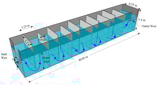
Figure 1.
Schematic view of full-scale chlorine contact tank (CCT) with dimensions.
2. Experimental Setup
A 1/10 scaled physical model of the CCT in Eskisehir Metropolitan Municipal WTP was constructed in the hydrodynamic laboratory of Civil Engineering Department at Eskisehir Osmangazi University. Froude number similitude was used to convert flow quantities from the prototype to model scale. The velocity and time scales were converted from prototype to model by the scale factor and discharge was converted by the scale factor in the Froude similitude. As shown in Figure 2, the experimental setup consisted of a stainless steel inlet tank, a polycarbonate contact tank with 15 mm thickness and 10 internal polycarbonate baffles with 10 mm thickness, a clean water tank, a sewage tank, galvanized transmission pipes 100 mm in diameter, an electromagnetic flow meter, and a centrifugal pump with a 1100 m3/h capacity. Supplied water from the network was passed through a filter system including washable granule carbon filters. The filtered water was collected in a clean water storage tank free of carbon and coarse waste. The flow discharge was adjusted using the valve located at the upstream of the inlet tank and measured using the LDG-100 electromagnetic flow meter, mounted in the middle of the transmission pipe to avoid local changes in the pipe flow. Water depth inside the contact tanks can be adjusted manually using the weirs located at the inlet and outlet of the contact tank. It should be noted that different water depths were measured in the contact tank depending on the energy head over the inlet weir for an adjusted flow rate. In order to diminish unsteady effects arising from the initial conditions, the flow was circulated between water storage tank and the CCT for 2 h before velocity measurements commenced.
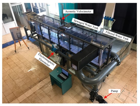
Figure 2.
Physical model and measurement system.
Turbulent flow velocities were measured using acoustic Doppler velocimetry (ADV) with a 25 Hz sampling rate in the sixth chamber of the CCT in order to exclude local changes in the flow originating from the inlet and outlet conditions. Measuring parameters of the ADV were carefully selected such that the signal to noise ratio (SNR) was greater than 20, which is recommended by the manufacturer [23]. One of the important parameters is the nominal velocity range (NVR), which can be regarded as the order of velocity magnitude to be measured. NVR was selected as the mean residence time (MRT) during experimental studies. The remaining parameters, such as transmit length (TL) and sampling volume (SV) were locally changed during the experimental studies since smaller SV and PL are required near the walls to reduce noise effects from the reflection of acoustic waves at the walls. Velocity measurements were carried out at 22 points over the chamber width at a constant elevation of water depth (y = h/2) to resolve the spatial variation of flow structure in the chamber. In order to observe flow features in the streamwise direction from the inlet to the outlet of the chamber, measurements were conducted at z+ = 0.25, 0.5, and 0.75, where the streamwise coordinate was non-dimensionalized with the length of the chamber. ADV measurements were carried out for 180 s at each point to collect adequate data for the time-averaged flow field inside the tank.
Tracer experiments were undertaken using Rhodamine WT Dye 20% concentrate. A 50 mL of 8 ppt concentration of Rhodamine WT solution was filled into syringes and injected using a syringe pump with six channels at the tank inlet during release time, which was determined according to the Froude number similitude. The tracer concentration was measured and recorded by using a Cyclops 7F fluorometer at the outlet of the ninth chamber. The injection capacity of the syringe pump allowed for conducting tracer experiment for winter flow rate. The valve at the inlet of the clean water tank was closed and the dye water was directed to the sewage tank to prevent mixing the dye with the clean water. The experimental results for the validation of the numerical model are given and discussed in the Section 4.1.
3. Computational Model
3.1. Flow Solver
Incompressible and turbulent flow inside the tank is described by the following Reynolds-averaged Navier–Stokes (RANS) equations:
where is the averaged velocity component in the i-direction (x, y, and z directions), is the averaged pressure, t is the time, ρ is the fluid density, υ is the kinematic viscosity, and xi and xj represent Cartesian coordinates. Turbulent flow in the real size CCT can be simulated using the k-ε turbulence closure model due to fully developed turbulent flow conditions with high Reynolds numbers [24], which is the reason for using the RANS approach in the present study. Reynolds stresses in the RANS approach can be approximated from the following Boussinesq hypothesis:
where represents Reynolds stresses, is the Kronecker delta, is turbulence kinetic energy, and is the turbulent viscosity, which can be calculated by
where is the turbulence dissipation rate and is selected as 0.09. In addition to the momentum equations, two transport equations are solved during flow simulations for the approximation of turbulence kinetic energy and dissipation rate.
3.2. Tracer Simulations
Tracer simulations are performed for a conservative tracer to assess the hydraulic and mixing performance of the present CCT. For the propagation of the tracer, the following advection-diffusion equation is numerically solved through the steady-state flow field:
where is the turbulent diffusivity and is calculated from the ratio of the turbulent viscosity , which is obtained from the flow solution, to the Schmidt number, which is defined as the ratio of the momentum diffusivity to mass diffusivity. In this study, the Schmidt number is set to 0.7 [17].
In the present study, a tracer is injected at the inlet of the tank as a pulse during release time. Zhang et al. [25] numerically showed that the release time should be kept at less than 5% of the MRT, which can be calculated from the ratio of the volume of the tank to the flow rate, as follows:
The water depth inside the tank was measured from the physical model and upscaled to the prototype for each flow rate since free-surface effects are neglected in the numerical simulations. MRT and injection time values are calculated and listed in Table 1 for seasonal water supplies.

Table 1.
Flow conditions for different seasons.
A numerical solver was developed based on OpenFOAM library for the solution of Equation (5) and employed for the simulation of the conservative tracer [26]. Hydraulic and mixing indexes were determined to rely on residence time distribution (RTD) plots, which were obtained from monitoring the tracer concentration at the outlet of the contact tank. The tracer concentration is non-dimensionalized as and the cumulative concentration observed at the outlet is calculated from , where is the injected tracer concentration, is the injection time, is the dimensionless time, and is the MRT.
3.3. Disinfection Modeling
Chlorine decay and pathogen inactivation during the disinfection process are governed by the following advection-diffusion equations with source terms:
where is the chlorine concentration , is first order decay rate of the chlorine depending on water temperature and pH level, N is the microorganism number, and is first-order pathogen inactivation rate for Giardia, since the dominant pathogen in raw water in the province of Eskisehir is Giardia. The empirical coefficients and were calculated for each season depending on pH level and temperature of raw water [10,27,28,29,30] and are listed in Table 1 for each season.
3.4. Mesh and Boundary Conditions
A block-structured mesh was generated using the standard utility blockMesh in OpenFOAM (Figure 3). In this approach, blocks are constructed inside the chambers and mesh is refined using appropriate refinement parameters, such that the mesh is fine enough near the solid boundaries in order to capture rapid variations in velocity and pressure due to the wall effects. A mesh independence study was performed using different mesh resolutions containing 1.23, 2.43, 4.86, 7.29, and 9.72 million cells and the results are compared in Figure 4. While coarse meshes produce mesh dependent variations especially near the walls, Mesh 4 and Mesh 5 gave identical results, which shows that the numerical solution is no longer dependent on the resolution of the mesh. The dimensionless cell size y+ near the wall is kept less than 11.6 to ensure that the first cell adjacent to the wall is in the viscous sublayer. The resultant mesh used in the present simulations consists of 9.72 million cells.
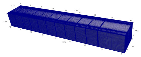
Figure 3.
Block-structured mesh for the full-scale contact tank.
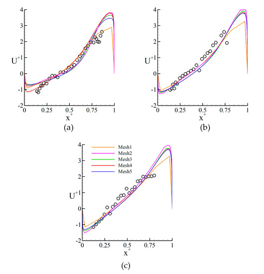
Figure 4.
Comparison of experimental and numerical velocity profiles in different streamwise locations: (a) z+ = 0.25, (b) z+ = 0.50, and (c) z+ = 0.75. Symbols represent measured and continuous line represents numerical data.
The appropriate boundary conditions were defined and used at the inlet, outlet, wall, and free-surface to mimic flow conditions in the real case. At the inlet, the average flow velocity is calculated from the ratio of the flow discharge to the inlet area and imposed as constant in the flow direction. Inlet boundary conditions for the turbulent flow are determined from the following equations [31]:
where is the average flow velocity at the inlet section; is the turbulence intensity, which is set to 0.05; and is the turbulence length scale. Free-stream boundary conditions are applied for all flow variables at the outlet of the computational domain to prevent the reflection of flow variables. No-shear condition is applied for the velocity and a zero gradient boundary condition is used for the pressure at walls. Unified wall functions are employed for the turbulence kinetic energy k, the specific turbulent dissipation rate ε, and the turbulent viscosity υt at the walls. Symmetry boundary condition is applied on the free-surface for all flow variables to impose slip effects since free-surface effects are neglected. Boundary conditions used in the numerical simulations are given in Table 2.
Table 2.
Boundary conditions.
Numerical simulations were performed using OpenFOAM on a high performance computing center with parallel computing. The entire computational domain is decomposed into 112 subdomains and each subdomain is solved on a different node during the computation. The use of open source code allowed us to develop new solvers for the simulations of conservative (Equation (5)) and reactive tracers (Equations (7) and (8)), as well as to perform computational runs on a cloud computing center located in Turkey.
4. Results and Discussions
4.1. Validation of the Numerical Model
A numerical simulation was performed on the model scale for the summer flow rate and the simulated steady-state flow velocities are compared with the measured velocities in Figure 4. Velocity components are non-dimensionalized with the plug flow velocity. Downlooking probes of the ADV did not allow us to approach and measure the flow velocities at points close to the baffles. As seen in Figure 4, the present numerical model can capture the spatial variations of flow velocities over the chamber width, even near the inlet and outlet of the chamber, at which unsteady variations are expected to be significant due to the energetic eddies forming near the corner of the baffles. The accuracy of the present numerical model reduces near the inlet and outlet of the chamber. This consequence is due to the inherent limitation of the RANS approach, since only the time-averaged values are considered in this approach. LES might remedy this drawback of the numerical model. However, this would require extremely high computational resources to resolve sub-grid scale eddies in such a large computational domain.
The jet velocity near the baffle reached 4U+, which is the indication of strong short-circuiting inside the chamber. Recirculating flows adjacent to the high velocity parcels resulted in negative velocities near the left wall of the chamber, which encompasses most of the chamber width, especially at z+ = 0.75, due to fact that the size of the recirculating zone increased as the flow approaches to the chamber outlet. The persistent formation of recirculating zones near the walls resulted in a narrow volume of mean flow and, consequently, the flow velocities increased significantly to pass the same flow rate in a smaller volume. Using the patented baffle design, both recirculating and dead zones converting to active mixing zones can remedy this problem, which is discussed in detail in the remainder of this study.
Tracer simulation was performed through the steady-state flow field. The simulated tracer concentration at the outlet of the ninth chamber is compared with the experimental measurement for non-dimensional RTD and cumulative RTD plots in Figure 5. A good agreement is achieved between the numerical and experimental results, which will eventually allow us to use the validated numerical model for the tracer simulation in real flow conditions.
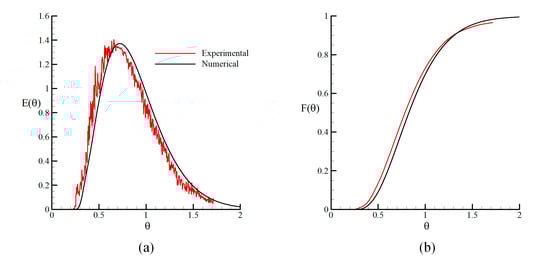
Figure 5.
Validation of numerical model of conservative tracer analysis (a) RTD (residence time distribution) and (b) cumulative RTD curves for winter.
4.2. Results for the Full-Scale CCT
Numerical simulations were performed for the flow characteristics and are given in Table 3. Convergence parameters of the steady-state flow conditions were selected as 1e-10 for , , and , 1e-12 for pressure. The steady-state flow conditions were achieved after 92,500 iterations for the summer condition due to the unsteady effects observed near the inlet and outlet.
Table 3.
Initial conditions.
The velocity vectors on the horizontal plane. located at the mid-depth of the tank, are shown for each season in Figure 6. Note that the velocity components are non-dimensionalized with respect to the plug flow velocity. As expected, flow structures were found to be identical in each season. The flow entering the tank with high velocity impinges on the wall of the entrance chamber and creates a complex flow structure at the upstream of the tank. A periodic flow structure evolves along the streamwise direction in the remaining chambers except in the last chamber due to local changes at the outlet weir. Recirculating flows formed by the turbulence and wall effects result in flow jets in each chamber, which are the indications of short-circuiting and a low hydraulic performance of the CCT. High flow velocities near the baffles also give rise to increased energy losses in the turbulent flow through the CCT.
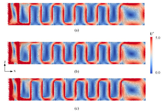
Figure 6.
Dimensionless velocity vectors at the horizontal plane for different seasons: (a) Summer, (b) spring, and (c) winter.
Tracer studies were carried out for the propagation of the conservative tracer through the steady-state flow field during three MRTs to allowed the total injected tracer to leave the computational domain, since a portion of the injected tracer may be trapped inside the recirculating zones. A control volume was created at the outlet of the tank and the volume-averaged value of the tracer concentration was monitored during the numerical simulations to obtain the RTD and cumulative RTD curves (Figure 7).
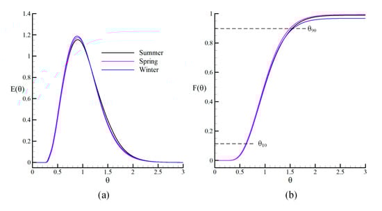
Figure 7.
(a) RTD and (b) cumulative RTD curves for each season.
Hydraulic and mixing efficiencies of the contact tank can be evaluated based on the baffling factor (θ10), Morrill (Mo), dispersion (σ), and AD indexes. The baffling factor θ10 refers to the dimensionless time required to observe 10% of the injected conservative tracer concentration at the outlet of the CCT. The Mo index is identified as the ratio of the θ90 value, that is the dimensionless time required to observe 90% of the tracer concentration at the outlet, to the θ10. The dispersion index is a statistical indicator for the evaluation of mixing efficiency, which can be calculated by the ratio of the variance of RTD curve to the square of the dimensionless time of the center of the RTD curve as . The AD index has recently been proposed by Demirel and Aral [19] for the appraisal of both hydraulic and mixing efficiencies in a CCT, since existing indicators may give confusing results for different tank and flow configurations. The AD index is defined as follows:
Detailed classifications of several contact systems can be found in Demirel and Aral [19] according to the recommended values of the AD index. The peak in the RTD curve corresponds to the bulk of the tracer concentration transport by the flow jet, observed in the velocity vectors in Figure 6. The higher value of the peak in the RTD plot implies the transport of more concentrated volumes of the tracer by the flow jet. In order to assess performance of the CCT, efficiency indexes were calculated based on the cumulative RTD plot in Figure 7b and listed in Table 4 for each season. The efficiency indexes are found almost identical since variations in flow discharge produce different flow depths in the tank. The hydraulic efficiency of the present CCT was classified as “average” according to the EPA standards [1]. Previous studies show that the mixing increases when Mo approaches to 2 [1], σ approaches to zero, and the AD index is greater than 3.5 [20]. Thus, the calculated indexes represent low mixing in the present CCT.
Table 4.
Hydraulic and mixing efficiency indexes.
The surface water treatment rule (SWTR), established by the United States Environmental Protection Agency (USEPA) in 1997, suggests 3-log (99.9%) for Giardia as a degree of inactivation, and 4-log (99.99%) for viruses. The degree of log-inactivation is evaluated by a logarithmic scale calculation, in which the degree of log-inactivation is determined by comparing the amount of pathogens in the raw water to the amount of pathogens in the treated water.
where is the initial amount of pathogen and is the amount of pathogen after the disinfection process. Thus, 3-log inactivation is achieved if the ratio of is 1000. The initial number of pathogens in the tank is set to unit and disinfection simulations were performed with continuous injections of chlorine concentration and pathogen at the inlet during θ [1]. Numerical simulations were repeated using different chlorine concentrations in order to determine at which chlorine concentration the 3-log inactivation can be achieved for a given temperature and pH level. As seen in Figure 8, the optimum chlorine demands were determined as 7, 8.5, and 13 mg/L for winter, spring, and summer conditions, respectively. While the hydraulic and mixing efficiencies of the CCT were not significantly influenced by the seasonal variations, the disinfection efficiency was found to be more responsive to the seasonal variations of temperature and pH level of the supplied water.
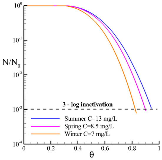
Figure 8.
Pathogen inactivation levels during one MRT.
4.3. Application of the SBD to the Full-Scale CCT
The low hydraulic and mixing efficiencies of the CCT lead to high chlorine demands for the pathogen inactivation, especially for the summer condition, since high water temperatures and low pH in summer months not only decrease the inactivation potential of the pathogen, but also increase the chlorine decomposition, which requires higher chlorine concentrations for the disinfection process. In order to enhance hydraulic and mixing efficiencies, as well as the disinfection performance of the CCT, recently patented SBD was then applied to the operating conventional tank design [32]. As shown in Figure 9, three slots were constructed on the baffle and located in the streamwise direction. Flow and tracer simulations were performed for various combinations of widths and locations of the slots to find the optimum configuration at which the efficiency becomes maximum [18]. A limited percentage of the flow discharge should be allowed to pass through the slots in this concept since higher flow discharges emerging from the slots may result in a violation of the flow-through-system. Different types of slot configurations can be applied, such as alternating slot widths in the streamwise direction [32].
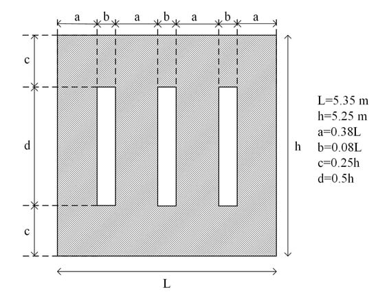
Figure 9.
The SBD concept.
The idea behind this novel SBD concept is to convert recirculating zones to the active mixing zones by using the momentum of the jet, as shown in Figure 10. The momentum transfer between the flow jet and dead zones in the neighboring chambers will also result in a considerable amount of reduction in the momentum of the jet. Several authors in the literature attempted to increase the efficiency of the contact system by including additional horizontal and vertical baffles, as well as alternating chamber widths [2,11,22,25]. Although such attempts have increased the hydraulic efficiency of the CCT, additional baffles increased the energy loses in the flow as well. The other contribution of the SBD is to reduce the energy loses in the turbulent flow through the CCT.
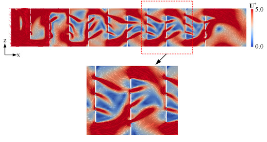
Figure 10.
Velocity vectors in the novel CCT design. Velocity vectors are colored using the magnitude of the velocity.
Tracer simulation was carried out for the SBD under summer conditions and the results are compared with the conventional design in Figure 11. The higher peak in the RTD plot for the SBD indicated that a greater amount of tracer contacted the water during the same contact time as in the conventional design, since short-circuiting effects were significantly suppressed. Efficiency indexes were calculated based on the cumulative RTD plot and are compared in Table 5 by the application of the SBD in order to assess the achievements. The hydraulic efficiency increased from “average” to “good” according to the baffling classification suggested by the U.S. EPA [1]. The Mo and dispersion index approached 2 and zero, respectively, which are recommended as perfect mixing system by the U.S. EPA [1]. The AD index also indicated an efficiency enhancement.
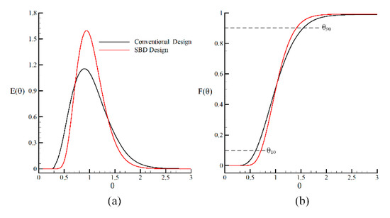
Figure 11.
Comparison of the tracer results for the conventional and SBD designs. (a) RTD and (b) cumulative RTD plots for summer conditions.
Table 5.
Hydraulic and mixing efficiency indexes for conventional and SBD designs.
Disinfection simulations were performed using different concentrations of chlorine to determine at which chlorine concentration the SBD could yield the 3-log inactivation level. As seen in Figure 12, the SBD can provide 3-log inactivation of pathogens using a 19% less concentration of chlorine than the conventional design, which is significant for the reduction of harmful effects of the chlorine to public health. This positive outcome is the result of an enhancement in both the hydraulic and mixing performance of the CCT, which are strongly connected features of the contact system. The conventional design could achieve a 2.75-log inactivation level when 10.5 mg/L chlorine concentration was used, which is another piece of evidence that the SBD has the better disinfection performance. The SBD and conventional designs exhibit distinct decay rates in pathogen inactivation during contact time, since short-circuiting effects observed in the conventional design cause the inactivation rate to drop sharply, which gives a smaller inactivation level during one MRT.
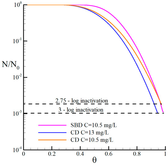
Figure 12.
Disinfection performance of slot-baffle design.
The CT (concentration-time) concept is practically used to determine the required chlorine concentrations in WTPs depending on the disinfectant residual concentration Cres (mg/L) and contact time T10 (min) [33,34]. Suggested CT values can be obtained from CT tables based on the inactivation level, residual chlorine concentration, pH level, and temperature [1]. The present simulations for the conventional design were T10 = 7.55 min and Cres = 6.32 mg/L. Thus, the CT value was calculated as 47.72 mg-min/L, which is consistent with the suggested value of 46 mg-min/L by the CT tables for pH = 7 and 25 °C [1]. On the other hand, the CT was calculated as 45.65 mg-min/L for the SBD, based on T10 = 8.83 min and Cres = 5.17 mg/L, which is close to the suggested CT value again. This result shows that the operator in a WTP can use existing CT tables for the SBD, depending on the modified T10 and measured Cres. However, CFD simulations need to be performed for the accurate prediction of the T10 for the SBD.
5. Conclusions
Hydraulic, mixing, and disinfection efficiencies of a full-scale CCT have been quantitatively analyzed using three-dimensional numerical simulations of turbulent flow and conservative tracers, as well as pathogen disinfection by chlorine. In order to validate the numerical model, laboratory studies were carried out in terms of velocity measurements and dye tracer studies on a scaled model of the CCT. The numerical model shows a good agreement with the experimental results for velocity profiles over the chamber length and dye concentration at the outlet. Numerical simulations of chlorine decay and pathogen inactivation yielded consistent results with the CT concept, which is practically used in the operation of WTPs. A recently patented SBD was then applied to the present CCT for efficiency enhancement. The following improvements have been achieved with the application of the SBD:
- Hydraulic performance was improved from “average” to “good” according to the baffling factor.
- Mo and dispersion indexes approached 2 and zero, respectively, which are suggested as perfect mixing systems by the regulations.
- As the hydraulic and mixing efficiencies improved, disinfection efficiency of the CCT was enhanced. The 3-log inactivation of Giardia cysts was achieved using 19% less chlorine dosage than the conventional design, which is significant for the reduction of harmful effects of the chlorine to public health.
- The energy efficiency of the CCT was improved by 62% according to the energy efficiency coefficient.
- The T10 can be obtained from the CFD simulations of the SBD and the required chlorine concentrations can be determined from CT concept for the calculated T10 and measured residual chlorine concentration at the outlet.
Author Contributions
Conceptualization, M.M.A. and E.D.; Methodology, M.A.K, E.D. and M.M.A.; Software, M.A.K. and E.D.; Validation, M.A.K. and E.D.; Formal Analysis, M.M.A., E.D. and M.A.K.; Investigation, M.M.A., E.D. and M.A.K.; Resources, M.A.K. and E.D.; Data Curation, M.A.K.; Writing-Original Draft Preparation, M.A.K., E.D.; Writing-Review & Editing, M.M.A.; Visualization, M.A.K.; Supervision, M.M.A.; Project Administration, E.D.; Funding Acquisition, E.D.
Funding
This research was funded by the Scientific and Technological Research Council of Turkey (TUBITAK) Grant No. 217M472.
Acknowledgments
The numerical calculations reported in this paper were fully performed at TUBITAK ULAKBIM, High Performance and Grid Computing Center (TRUBA resources).
Conflicts of Interest
The authors declare no conflict of interest.
References
- US EPA. Disinfection Profiling and Benchmarking Guidance Manual; Appendix A Rep. No. EPA 816-R-03-004; EPA: Washington, DC, USA, 2013.
- Gualtieri, C. Analysis of the effect of baffles number on a contact tank efficiency with Multiphysics 3.3. In Proceedings of the COMSOL User Conference, Napoli, Italy, 23–24 October 2007. [Google Scholar]
- Rauen, W.B.; Lin, B.; Falconer, R.A.; Teixeira, E.C. CFD and experimental model studies for water disinfection tanks with low Reynolds number flows. Chem. Eng. J. 2008, 137, 550–560. [Google Scholar] [CrossRef]
- Teixeria, E.D.; Siqueira, R.N. Performance assessment of hydraulic efficiency indexes. J. Environ. Eng. 2008, 134, 851–859. [Google Scholar] [CrossRef]
- Wilson, J.M.; Venayagamoorthy, S.K. Evaluation of hydraulic efficiency of disinfection systems based on residence time distribution curves. Environ. Sci. Tech. 2010, 44, 9377–9382. [Google Scholar] [CrossRef] [PubMed]
- Amini, R.; Taghipour, R.; Mirgolbabaei, H. Numerical assessment of hydrodynamic characteristics in chlorine contact tank. Int. J. Numer. Methods Fluids 2011, 67, 885–898. [Google Scholar] [CrossRef]
- Zhang, J.; Tejada-Martínez, A.E.; Zhang, Q. Evaluation of large eddy simulation and RANS for determining hydraulic performance of disinfection systems for water treatment. J. Fluids Eng. 2014, 136, 121102. [Google Scholar] [CrossRef]
- Zhang, G.; Lin, B.; Falconer, R.A. Modelling disinfection by-products in contact tanks. J. Hydroinform. 2000, 2, 123–132. [Google Scholar] [CrossRef][Green Version]
- Zhang, J.; Huck, P.M.; Anderson, W.B.; Stubley, G.D. A computational fluid dynamics based integrated disinfection design approach for improvement of full-scale ozone contactor performance. Ozone Sci. Eng. 2007, 29, 451–460. [Google Scholar] [CrossRef]
- Angeloudis, A.; Stoesser, T.; Falconer, R.A. Predicting the disinfection efficiency range in chlorine contact tanks through a CFD-based approach. Water Res. 2014, 60, 118–129. [Google Scholar] [CrossRef]
- Angeloudis, A.; Stoesser, T.; Gualtieri, C.; Falconer, R.A. Contact tank design impact on process performance. Environ. Model. Assess. 2016, 21, 563–576. [Google Scholar] [CrossRef]
- Teixeria, E.C. Hydrodynamic Process and Hydraulic Efficiency of Chlorine Contact Units. Ph.D. Thesis, University of Bradford, Bradford, UK, 1993. [Google Scholar]
- Zhang, J.; Tejada-Martinez, A.E.; Zhang, Q.; Lei, H. Evaluating hydraulic and disinfection efficiencies of a full-scale ozone contactor using a RANS-based modeling framework. Water Res. 2014, 52, 155–167. [Google Scholar] [CrossRef]
- Carlston, J.S.; Venayagamoorthy, S.K. Impact of modified inlets on residence time in baffled tanks. J. AWWA 2015, 107, E292–E300. [Google Scholar] [CrossRef]
- Wang, H.; Shao, X.; Falconer, R.A. Flow and transport simulation models for prediction of chlorine contact tank flow-through curves. Water Environ. Res. 2003, 75, 455–471. [Google Scholar] [CrossRef] [PubMed]
- Edwards, E.S.; Anderson, W.B.; Andrews, S.A.; Huck, P.M. Disinfection assessment in full-scale chlorine contact chambers. J. Environ. Eng. Sci. 2002, 1, 311–322. [Google Scholar] [CrossRef]
- Kim, D.; Stoesser, T.; Kim, J.H. The effect of baffle spacing on hydrodynamics and solute transport in serpentine contact tanks. J. Hydraul. Res. 2013, 51, 558–568. [Google Scholar] [CrossRef]
- Aral, M.M.; Demirel, E. Novel slot-baffle design to improve mixing efficiency and reduce cost of disinfection in drinking water treatment. J. Environ. Eng. 2017, 143, 06017006. [Google Scholar] [CrossRef]
- Demirel, E.; Aral, M.M. An efficient contact tank design for potable water treatment. Tech. J. 2018, 29, 8279–8294. [Google Scholar] [CrossRef]
- Demirel, E.; Aral, M.M. Performance of efficiency indexes for contact tanks. J. Environ. Eng. 2018, 144, 04018076. [Google Scholar] [CrossRef]
- Kizilaslan, M.A.; Demirel, E.; Aral, M.M. Effect of porous baffles on the energy performance of contact tanks in water treatment. Water 2018, 10, 1084. [Google Scholar] [CrossRef]
- Zhang, J.; Tejada-Martinez, A.E.; Zhang, Q. Indicators for technological, environmental and economic sustainablity of ozone contactors. Water Res. 2016, 101, 606–616. [Google Scholar] [CrossRef]
- Nortek, A.S. VECTRINO Velocimeter User Guide (Rev. C); Nortek Scientific Acoustic Development Group Inc.: Vangkroken, Norway, 2004. [Google Scholar]
- Wang, H.; Falconer, R.A. Simulating disinfection process in chlorine contact tanks using various turbulence models and high-order accurate difference schemes. Water Res. 1998, 32, 1529–1543. [Google Scholar]
- Zhang, J.; Pierre, K.C.; Tejada-Martiner, A.E. Impacts of flow and tracer release unsteadiness on tracer analysis of water and wastewater treatment facilities. J. Hydraul. Eng. 2019, 145, 04019004. [Google Scholar] [CrossRef]
- OpenFOAM. OpenFOAM User Guide; OpenCFD Ltd.: Bracknell, UK, 2015. [Google Scholar]
- Chick, H. An investigation of the laws of disinfection. J. Hyg. 1908, 8, 92–158. [Google Scholar] [CrossRef] [PubMed]
- Watson, H.E. A Note on the variation of disinfection with change in the concentration of the disinfectant. J. Hyg. 1908, 8, 536–542. [Google Scholar] [CrossRef] [PubMed]
- Clark, R.M. Modeling inactivation of Giardia Lamblia. J. Environ. Eng. 1990, 116, 837–853. [Google Scholar] [CrossRef]
- Brown, D.; Bridgeman, J.; West, J.R. Predicting chlorine decay and THM formation in water supply systems. Rev. Environ. Sci. Biotechnol. 2011, 10, 79–99. [Google Scholar] [CrossRef]
- Turbulence Free-Stream Boundary Conditions. Available online: https://www.cfd-online.com/Wiki/Turbulence_free-stream_boundary_conditions (accessed on 18 July 2019).
- Aral, M.M.; Demirel, E. A Multi-Chamber Slot-Baffle Contact Tank Design; European Patent Office: Munich, Germany, 2019; in press. [Google Scholar]
- Lev, O.; Regli, S. Evaluation of ozone disinfection systems: Characteristic concentration C. J. Environ. Eng. 1992, 118, 477–494. [Google Scholar] [CrossRef]
- Lev, O.; Regli, S. Evaluation of ozone disinfection systems: Characteristic time T. J. Environ. Eng. 1992, 118, 268–285. [Google Scholar] [CrossRef]
© 2019 by the authors. Licensee MDPI, Basel, Switzerland. This article is an open access article distributed under the terms and conditions of the Creative Commons Attribution (CC BY) license (http://creativecommons.org/licenses/by/4.0/).