Article

CFD Optimization Process of a Lateral Inlet/Outlet Diffusion Part of a Pumped Hydroelectric Storage Based on Optimal Surrogate Models

1
State Key Laboratory of Hydraulic Engineering Simulation and Safety, Tianjin University, Tianjin 300072, China
2
China Water Resources Beifang Investigation, Design and Research Co. Ltd. (BIDR), Tianjin 300072, China
*
Author to whom correspondence should be addressed.
Processes 2019, 7(4), 204; https://doi.org/10.3390/pr7040204
Submission received: 5 March 2019 / Revised: 2 April 2019 / Accepted: 4 April 2019 / Published: 10 April 2019

Abstract

:
The lateral inlet/outlet plays a critical role in the connecting tunnels of a water delivery system in a pumped hydroelectric storage (PHES). Therefore, the shape of the inlet/outlet was improved through computational fluid dynamics (CFD) optimization based on optimal surrogate models. The CFD method applied in this paper was validated by a physical experiment that was carefully designed to meet bidirectional flow requirements. To determine a good compromise between the generation and pump mode, reasonable weights were defined to better evaluate the overall performance. In order to find suitable surrogate models to improve the optimization process, the best suited surrogate models were identified by an optimal model selection method. The optimal configurations of the surrogate model for the head loss and the velocity distribution coefficient were the Kriging model with a Gaussian kernel and the Kriging model with an Exponential kernel, respectively. Finally, a multi-objective surrogate-based optimization method was used to determine the optimum design. The overall head loss coefficient and velocity distribution coefficients were 0.248 and 1.416. Compared with the original shape, the coefficients decrease by 6.42% and 40.28%, respectively. The methods and findings of this work may provide practical guidelines for designers and researchers.

1. Introduction

In recent decades, many electricity generation problems have been caused by their high production cost and environmental impact [1]. It is generally accepted that renewable energy can provide promising solutions for the problems, and much research has been focused on numerous techniques, such as hydropower [2,3,4], fuel cells [5], biofuels [6], wind power [7,8,9], and solar power generation [10]. Pumped hydroelectric storage (PHES) has attracted widespread interest because of its great flexibility and storage capacity in improving grid stability of other renewable energy sources [11,12]. The lateral inlet/outlet plays a critical role in the connecting tunnels of the water delivery system in a PHES, and its flow conditions can affect the economic benefit and operation stability of the PHES to a great extent. The PHES operates under pumped or generation conditions according to the command, and the water flows between the upper and lower reservoir through the inlet/outlet. Compared with ordinary hydropower stations, the hydraulic requirements for the inlet/outlet structure of the PHES require more attention.
Much research in recent years has focused on the hydraulic performances of the inlet/outlet experimentally and numerically. Müller et al. [13] carried out prototype measurements by Acoustic Doppler Current Profiler (ADCP) to study flow velocities in the reservoir; subsequently a numerical model was built to further understand the flow development near the inlet/outlet. In order to ensure satisfactory hydraulic performances, Bermúdez et al. [14] conducted numerical and physical model studies on the inlet/outlet of the Belesar-III power station in Northwest Spain. The initial design was optimized by numerical method, and the new design presented a more homogenous flow distribution and a reduced head loss. Cai et al. [15] performed an experimental study on the effects of the shape and position of separation piers on the flow characteristics with two operations. Gao et al. [16] tried to improve the velocity distribution at the intake-outlet orifices through 20 types of shape optimization experiments. Sun et al. [17] found the incorrect arrangement of separation piers probably contributes to disadvantageous velocity distribution for the trash rack. Ye et al. [18] simulated turbulent flow in a lateral inlet/outlet to explore the diffusion segment shape that can obtain better velocity and discharge distributions. Based on the validation of the experiment, flows in the lateral inlet/outlet were numerically simulated focusing on the variations in discharge distributions over different orifices; the results showed that the flow non-uniformity was improved successfully by adjusting the diffusion segment and width between the separation piers [19]. The investigations indicate that computational fluid dynamics (CFD) has been used frequently to optimize the structure parameters of the inlet/outlet that can easily influence the hydraulic objectives. However, the process mentioned above is a trial-and-error approach requiring intensive work and a lot of time [20], and the results may be subjective to some extent.
CFD coupled with optimization techniques has been used to determine the best design scheme for wind turbine devices [21,22,23], and the adopted methods provide a reference for inlet/outlet optimization. For complex optimization problems, two methods have been generally applied to achieve optimization. When there are many individual objective functions, the functions can be combined into a single composite one; nonetheless it can be difficult to determine the proper and typical selection of the weights. In addition, the combination method would provide only a single result that cannot be chosen to make a trade-off. Therefore, multi-objective evolutionary algorithms (MOEAs) are more desired by decision makers. For MOEAs, it is common to use the concept of Pareto solutions. Pareto solutions consist of many non-dominated solutions where some gain in objectives always causes some sacrifice to others. MOEAs, such as Non-dominated Sorting Genetic Algorithm II (NSGA-II) [24,25], can offer many Pareto results in one single simulation process and have been extensively applied in engineering optimization.
Although MOEAs can obtain many solutions, these algorithms also require an even larger number of simulations and an unacceptable computation time in practice. Thus, multi-objective optimization based on the surrogate methods is receiving increasingly more support and attention. These approaches present objective functions by surrogate models, replacing expensive high-fidelity design simulations. The model is an effective engineering technique that can considerably save computing expense while still providing reasonably accuracy. Therefore, the multi-objective surrogate-based optimization method makes it more feasible to perform exhaustive global searches in the design space for complicated shape optimization. The optimization result will be more satisfactory because the exploration is not subjected to a limited number of simulating data and computing resources. General surrogate models contain Response Surface Methodology (RSM) [26,27], Radial Basis Function (RBF) [28,29,30,31,32], and Kriging [33,34,35]. However, owing to the diverse functional characteristics of the popular models, it is important to choose the most appropriate models for the responses of hydraulic objectives to diffusion segment parameters. For that reason, a recently surrogated model selection method proposed by Mehmani et al. [36], called the Concurrent Surrogate Model Selection (COSMOS), was adopted to construct suitable models in this paper.
Although a multi-objective CFD optimization process for the inlet/outlet was developed in previous works [37,38], there are some drawbacks in the original process: (1) The CFD method was indirectly validated only by comparing the result with that of a published reference [18], which weakened the reliability of the optimization process. (2) Only a single surrogated model (RSM) was considered to accelerate the optimization procedure. However, there is no universal surrogate model for every practical problem, and suitable model selection is critical for accuracy. (3) The objectives for the pump and generation mode were simply added up to estimate the total performance. Nevertheless, the significance of the pump mode and generation mode is probably not equal in many cases. Therefore, in this study a physical model experiment was well-designed to meet the requirement of bi-directional flow, and a more extensive validation of the CFD model was performed. Based on the validated CFD model, the COSMOS method was applied to select suitable surrogate models for the objectives of the inlet/outlet, to further improve the accuracy of the original optimization process. In addition, in order to better evaluate the overall hydraulic performance, the selection of objective functions was reconsidered and weight coefficients of different operation modes were introduced. In the present article, the shape of an inlet/outlet was improved through CFD optimization based on optimal surrogate models. The aim of this work was to apply the optimal surrogate optimization process to determine the optimum shape of the inlet/outlet, to simultaneously obtain better hydraulic performances under bidirectional flow conditions.

2. Problem Description

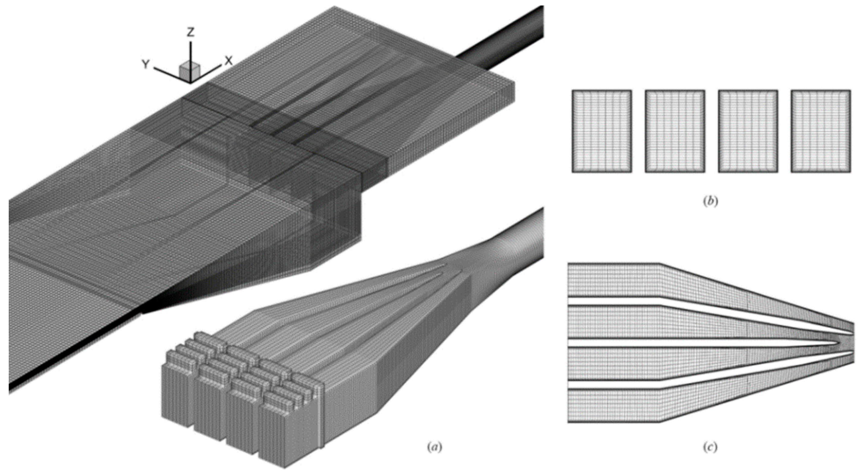
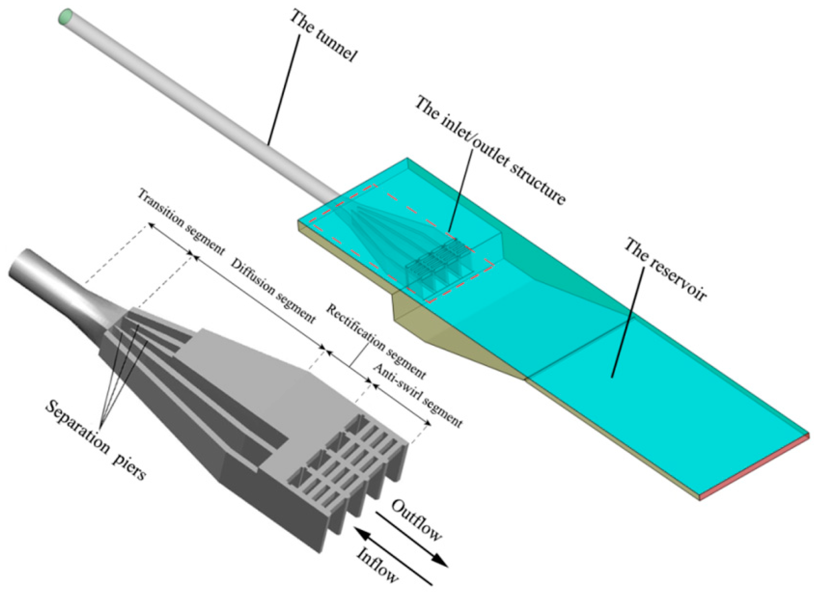
The typical shape of the lateral intake is shown in Figure 1. When the PHES is in the generation mode, water flows into the lower reservoir through the tunnel and the inlet/outlet structure. Because water flows out from the inlet/outlet in this mode, the phenomenon is also called “outflow”. Along the outflow direction, the structure generally contains a transition part (a structure connecting a circular cross-section tunnel and a diffusion part), a diffusion part, a rectification part, and an anti-swirl part.
The diffusion part is very sensitive to the performance of the intake, and it is generally improved for the structure design. 
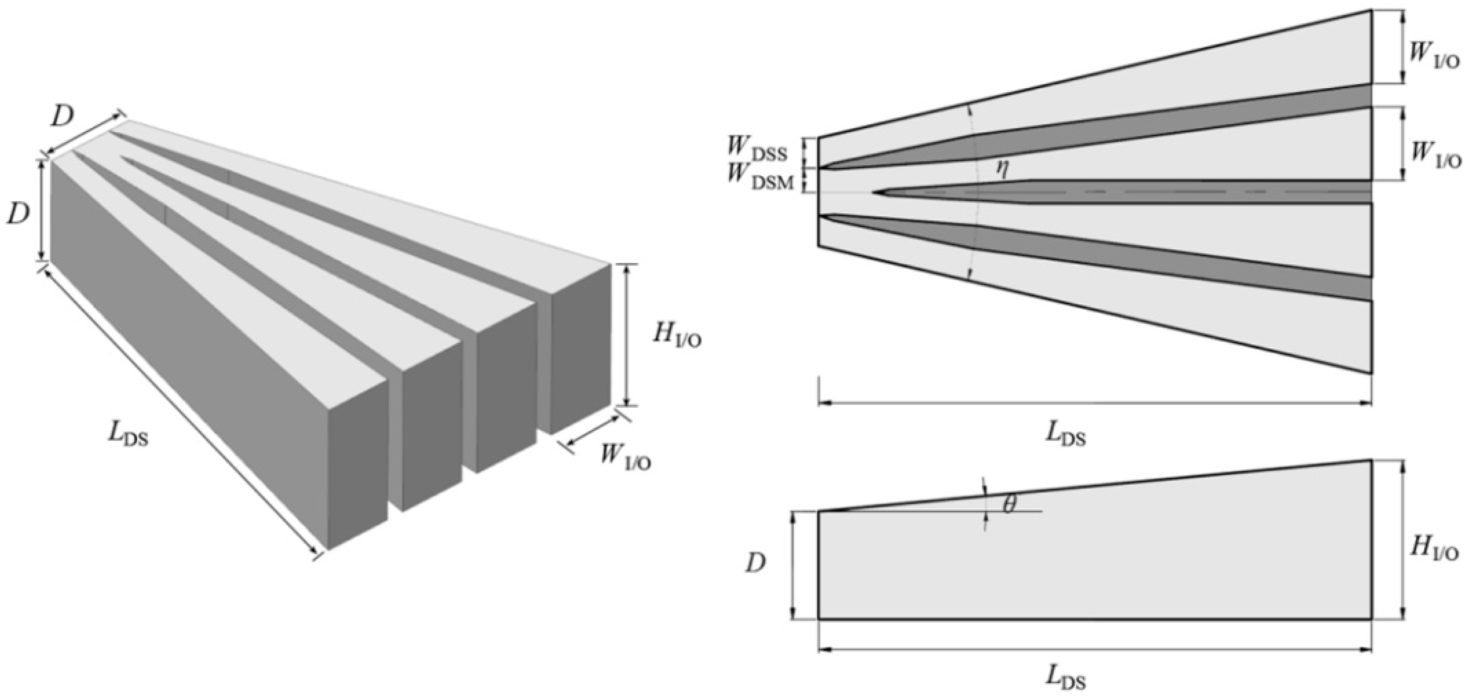
Figure 2 present flow passages and basic parameters in the diffusion part. This parameters include the length of the diffusion part (LDS),height of the inlet/outlet orifices (HI/O),wide of the separation pier in the middle orifices (WDSM),width of the separation pier in the side orifices (WDSS),horizontal diffusion angle ( η ), and vertical angle ( θ ). The left side displays the 3D model for the flow passage. On the right side, plane sections of the model are demonstrated, and the flow passage and separation piers are marked out with light grey and dark grey, respectively. It should be noted that the tunnel diameter D in the PHES is generally decided beforehand by the difference of the water head between the upper and lower reservoir, the installed capacity of turbines, topographic and geological conditions etc. For the inlet/outlet optimization, the value of D is fixed (D = 7.2 m in the current study) because a change may need adjustment of the whole layout of the water conveyance system resulting in excessive costs. Besides, the number of orifices (4) is also fixed in view of it being the most commonly used form of the lateral inlet/outlet in the PHES of China. For more information about the shape parameters, readers can refer to the previous work [38].
The lateral inlet/outlet hydraulic performance is characterized by three parameters: the head loss, the velocity, and the flowrate distribution [37,38,39]. According to the Bernoulli equation, the head loss is computed as:
h 0 - 1 = 0 1 α v 2 2 g
h 1 - 0 = 1 0 + α v 2 2 g
ξ = 2 g h f α v 2
where the head loss h f = h 0 - 1 and h f = h 1 - 0 are used for the inflow and outflow mode, respectively; ξ is the coefficient of the head loss; 0 and 1 are the piezometric head in the reservoir and tunnel; v is the bulk velocity at the boundary of the tunnel; α is the kinetic energy correction coefficient.
Numerous vibration-caused trash rack failures have occurred because the trash rack may be exposed to high velocities at the orifice cross-section [40]. Hence C V is proposed as a typical index evaluating the uniformity of the flow velocity at orifices [39,41], and a lower C V implies a better velocity distribution in the inlet/outlet. Considering there are four orifices divided by the separation pier, C V could change with different orifices due to the influence of horizontal diffusion. In order to represent the overall performance of the velocity distribution, the worst case i.e., the maximum value of C V among the four orifices, is selected. Thus C V is defined as:
C V = max ( v max , i v i )
where v max is the maximum value among the velocities at the orifice cross-section; i indicates the index of orifices; v indicates the average velocity at the orifice cross-section.
In order to further improve the discharge distribution in the horizontal direction, the separation piers are designed to divide the flow passage into sub-tunnels. Then C Q is used to estimate the degree of flux uniformity by comparing the discharge between adjacent orifices, which can be defined as:
C Q = max ( Q i , i + 1 ) min ( Q i , i + 1 ) min ( Q i , i + 1 ) × 100 %
where Q i indicates the rate of flow at the different orifices (i = 1, 2, 3).
For the purpose of determining a good compromise between the two modes of operation, these parameters under inflow and outflow conditions should be carefully combined. In a recent study, Gao et al. [38] simply added up the parameters for the pump mode and the generation mode to estimate the total performance. However, the performance of the generation mode is probably more significant than that of the pump mode in many cases. The pumped water can be stored in the upper reservoir under the pump mode during the low load period of the power grid, while under the generation mode the water will flow into the lower reservoir to generate electricity during the peak load period. Designers tend to pay more attention to the head loss under the generation mode in order to achieve higher economic benefits. Therefore, a more reasonable approach is to use weights to deal with the combinations of the two modes. For that reason, the new combined objectives to evaluate the overall performance of the inlet/outlet are defined as follows:
ξ total = ω 1 ξ in + ω 2 ξ out
C V , total = ω 1 C V , in + ω 2 C V , out
where ξ total and C V , total are the overall head loss coefficient and velocity distribution coefficient, respectively; ω 1 and ω 2 are the weight coefficients of the objective function under the conditions of inflow and outflow, and ω 1 + ω 2 = 1 . In this article, the values of ω 1 and ω 2 are taken as 0.33 and 0.67 based on the specific engineering designer’s suggestion. However, they can be flexibly selected according to different projects.
Another drawback of their study [37,38] is the definition for the overall C Q , which is expressed as the difference of C Q between the pump and generation mode. C Q , in is the discharge uneven distribution coefficient under inflow condition, C Q , out is the discharge uneven distribution coefficient under outflow condition. When it is regarded as an objective function, it seeks to minimize the difference between C Q , in and C Q , out , rather than C Q , in and C Q , out themselves. If there are some bad points in the design space, on which the values of both C Q , in and C Q , out may be large, the difference (i.e., the overall C Q ) may be small. Besides, according to the guideline the discharge distribution is sufficiently uniform when C Q is less than 10% [39]. As a result it is more appropriate to choose C Q as the constraint, and the head loss and velocity distribution ( ξ total , C V , total ) can be optimized more flexibly.
Therefore, the objective functions were set to find the minimum values for ξ and C V , while C Q , η, and θ were treated as constraint conditions. Table 1 lists the design parameters and constraints in this study.

3. Numerical Model and Validation

3.1. Numerical Model

Figure 3 shows a detailed view of the structured grids in the research area. To increase the accuracy of the simulation, boundary layer grids were added to ensure that the dimensionless wall distance y+ of the first points near the walls was between 30 and 300. The distribution of y+ values for the inlet/outlet is shown in Figure 4.
Considering the accuracy and efficiency of the CFD simulations, it is important to work out a reasonable number of mesh elements [42,43,44]. Based on a previous grid independence study [38], a grid amount of 1.4 × 10⁶ was sufficient for CFD simulation, and similar grid sizes were thus adopted in this article.
As presented in Figure 1, a three-dimensional computational domain far larger than the inlet/outlet structure was developed to accurately simulate the flow pattern in the inlet/outlet. As to the boundary conditions, a uniform velocity was prescribed at the tunnel boundary, and a pressure condition was imposed at the reservoir boundary. The flow discharge changed slightly according to the operating conditions of the reversible turbines. A summary of boundary conditions for the Computational Fluid Dynamics (CFD) case under the generation and pump mode is listed in Table 2.
In the present study, the Reynolds Averaged Navier Stokes (RANS) equations were solved using ANSYS Fluent 17.0 [45]. The simulation was performed in a segregated manner adopting the realizable k-ε model combined with the wall function. The Navier–Stokes equations were solved by means of pressure implicit with splitting of the operator’s algorithm, and a second-order upwind method was employed to realize the discretization. The converged solution was obtained after the residual levels became less than 1 × 10⁻⁴. For detailed information about the governing equation and numerical settings, the reader can refer to references [38,45,46].

3.2. Experimental Setup

The CFD method in the original study [38] was validated by comparing the result with that of a published reference [18]. Although the results were found to be in good agreement, there were obvious differences in the velocity distribution between the case in the reference [18] and the case in this study, which weakened the reliability of the validation in the original study. Therefore, the CFD method still needs to be validated further, and a physical model experiment adopting a scale of 1/60 was conducted in this paper. As shown in Figure 5, an experimental setup was established which was 5.2 m long, 1.2 m wide, and 0.6 m high.
In order to show the experiment more clearly, the side view of the layout plan is illustrated in Figure 6. Control valves and electromagnetic flowmeters with an accuracy of 0.5% for the measured ranges were used to control the flow discharge. By switching the different control valves, bidirectional flow conditions could be realized in the experiment. In the inflow condition, the inflow control valves were open, while the outflow control valves were closed. Water from the high constant-head tower flowed into the reservoir channel through the pipe. Before the water entered the channel, a device was set up to align the flow pattern. Finally water flowed into a lower collecting tank, from which it was pumped back to the constant-head tank using a centrifugal pump. While in the outflow condition, the inflow control valves were closed, and the outflow control valves were open. Water was conveyed to the reservoir tank through a horizontal pipe with a length 50D that was long enough to guarantee full development of the flow in the pipe. The discharge in the inflow condition was 4.359 L/s, corresponding to a Reynolds number Re = 46,277 in the tunnel; while in the outflow condition, the discharge was 5.795 L/s and the Reynolds number was 61,519.
A Vectrino ADV instrument, developed by Nortek AS, was used to instantaneously measure stream-wise velocity of the diversion orifices at various depths. Based on the Doppler shift principle, the ADV instrument can measure velocities with ±1% accuracy in a measurement range of 1 mm/s. Each measurement point with a sampling volume of 7 mm worked at a sampling frequency of 50 Hz for 60 s of sampling time.

3.3. Validation of the CFD Model

The head loss coefficient in the inflow condition is obviously smaller than that in the outflow condition. In the inflow condition, the coefficients obtained from numerical simulation and experiment were 0.164 and 0.171 respectively, and their relative error was 4.09%. The coefficients of the simulation and experiment in the outflow condition were 0.315 and 0.338, and the relative error was 6.81%. Comparing the simulation results with the experimental data, although the numerical model slightly underestimates the coefficients, it is still acceptable to predict the results of the head losses.
For the purpose of comprehensively comparing the velocity distribution at the orifice cross-section (x = 10 m), there are three measured lines with equal distance at each orifice. As shown in Figure 7, the velocity data are obtained along the measured lines (A—A, B—B and C—C) at the cross-section.
Figure 8 and Figure 9 compare the numerical solutions with the experimental ones for the velocity distribution in both conditions. In the legend, M and S indicate the middle and side orifice, respectively; A, B, and C indicate the measured lines A—A, B—B, and C—C, respectively. For example, M-A represents the measured line A—A at the middle orifice. The y-axis indicates the relative height of the measured point normalized by the orifice height H, and the x-axis indicates the relative velocity also normalized by the average velocity of the measured line.
Figure 8a demonstrates that a good matching between the two approaches is obtained in the middle orifice. The results of both methods show that velocities among the three lines are very close to each other, and the distribution is also uniform along the height. In the side orifice, the numerical results are also in good agreement with the experimental ones. There are only slight differences in the velocity distribution among the measured lines. Compared with the flow pattern in the middle orifice, the more obvious change is that the mainstream appears at the lower part of the orifice, and the range of y/H is about 0.13–0.52.
While in the outflow condition, differences of the velocity distribution among the measured lines are also small in the side orifice. However, in the middle orifice the experimental results show that there are obvious differences among the velocities of three measured lines, which is also predicted by the simulation. In addition, the velocity distribution along the height is also not uniform, and negative velocities are generated at the top. For the M-B line, the y/H range of the negative region obtained from the experiment is about 0.8–1.0, and the numerical range is about 0.7–1.0. This difference is partly due to errors caused by the limited number of measured points in the experiment, and partly due to the slight overestimation for the strength of flow separation by the simulation. At the bottom of the orifice, the mainstream in the experiment is located a little higher than that in the simulation. Although there are some minor deviations in the outflow velocity distribution, the agreement is quite acceptable considering that the more complex flow separation occurs in the outflow condition.

4. Optimization Methodology

4.1. Surrogate Models Selection

The optimization algorithm coupled with the computationally intensive simulation requires intensive work and a lot of time. It is necessary to adopt the surrogate model because the CFD-optimization procedure requires too many computing resources, which weakens its application in practice. Therefore, surrogate models are employed to engage the optimization procedure in the paper. There are several surrogate model types as listed in Table 3, such as Response Surface Methodology (RSM), Radial Basis Function (RBF), and Kriging, which have been extensively used in recent years to solve engineering optimization design. Unlike other approaches, RSM applies simple algebraic expressions to generate the function relationship, and it is very suitable for complex engineering applications [47]. In addition, RBF has the best approach for high dimensionality optimization problems according to a literature survey [48]. For low dimensional optimization problems, the Kriging method can achieve good results in both accuracy and time. According to a survey of popular surrogate models in similar situations, RSM, RBF, and Kriging are considered as surrogate candidates in the researches.
When employing the surrogate model in the hydraulic optimization procedure, the challenge is how to create a model which is as accurate as possible. As mentioned above, RSM, RBF, and Kriging can be used to generate surrogate models, and their parameters are listed in Table 4. The kernel function and hyper-parameter also need to be chosen carefully, which requires an effective surrogate model selection method.
As we know, existing surrogate model selection methods generally contain three levels: selecting a model type, selecting a kernel function, and optimizing the hyper-parameters. Some researchers have used different error measures to separately select the model type, kernel function, or hyper-parameter [56,57,58]. With the intention of performing thorough selection, the Predictive Estimation of Model Fidelity (PEMF) was suggested by Mehmani et al. [59]. Furthermore, Mehmani et al. [36] advanced the Concurrent Surrogate Model Selection (COSMOS) on the foundation of the PEMF, and applied it to select suitable models by minimizing the model error. The error selection criterion is based on different situations and preferences. For the exploration of design space and parameter analysis, the median error can be used. On the other hand, it is more appropriate to choose the conservative maximum error for the structural safety optimization (e.g., to model vehicle crash simulation). Therefore, these criteria might be mutually conflicting or mutually promoting [36]. Considering the optimization for the hydraulic performance of the inlet/outlet may have certain requirements for the above two situations, the median and maximum errors of the surrogate model are treated as two selection criteria estimated by the PEMF method. Moreover, the framework will solve the multi-objective problem (minimizing the errors) to find the optimal models through the One-Step technique. In the technique, a single mixed integer nonlinear programming problem (MINLP) can be solved by the NSGA-II. Considering different models have different numbers of kernels and hyper-parameters, the candidates are classed as three smaller categories according to the hyper-parameters [36]. The computation of the Kriging model is performed with the MATLAB toolbox DACE [60], as it has been widely used in many applications concerning the Kriging model. The problem is usually anisotropic, which is accounted for in the construction of the surrogate models.

4.2. Optimization Algorithm

Extensive literature based on the NSGA-II [61] has been reported in engineering applications (listed in Table 3), which is also chosen for this investigation. In NSGA-II, a random parent population is initially produced, and individuals are sorted according to rank and crowding distance. Then the optimum resolutions are chosen to generate offspring populations using genetic operators that are the same in the standard GA. Specifically, a binary tournament selection, Simulated Binary Crossover (SBX) and polynomial mutation are employed in NSGA-II. SBX simulates the binary crossover observed in nature, and the crossover distribution index determines how far away the children solutions are from their parents [62]. Deb et al. [63] suggested a polynomial mutation operator with a mutation distribution index that can control the amount of perturbation in a variable. Table 5 lists the parameters for the optimization process.
To pick the optimum point from the Pareto frontier, Technique for Order Preference by Similarity to Ideal Solution (TOPSIS) is implemented in this article. TOPSIS, proposed by Hwang et al. [64], is a ranking method that can rank possible solutions on the Pareto frontier and select a trade-off optimum by measuring Euclidean distances.

4.3. Optimization Process Scheme

The multi-objective optimization process is built by combining the CFD numerical simulation, the design of experiment (DOE), the surrogate model selection based on the COSMOS, and the optimization method NSGA-II. The flow diagram of the process is presented in Figure 10.
First, the Optimized Latin Hypercube Sampling (OLHS) algorithm is applied in the Design of Experiment (DOE) to choose representative points. Then sample points are simulated using the CFD method, and the results are exacted to evaluate the objectives of the hydraulic performance. Based on the database of the DOE, a suitable surrogate model is constructed using COSMOS to improve the optimization efficiency and precision. The different surrogate models, such as RSM, RBF, and Kriging, are generated until the PEMF is deemed acceptable. Finally, NSGA-II is adopted to conduct the optimization. If the objective function does not change, or the maximum iteration number is reached, the optimization is terminated. Otherwise, the process will continue to loop with a new set of proposed design parameters.

5. Results and Discussion

5.1. Optimal Surrogate Models

In the present study, COSMOS is applied to choose the appropriate surrogate models. First of all, OLHS as an efficient sampling strategy is applied in DOE sampling, in which 60 points are randomly selected to construct these surrogate models. The Predictive Estimation of Model Fidelity (PEMF) method is chosen to check the accuracies of these surrogate models.
By solving the MINLP problem with NSGA-II, the final results of the models for ξ , C V , C Q , in and C Q , out are presented in Figure 11. Φi indicates the surrogate models containing i hyper-parameter(s). βH, βL, and βW indicate the correlation parameter of the design variable HI/O, LDS, and WDSM, respectively. A Pareto frontier is provided in each figure, and a trade-off solution is selected under comprehensive consideration of median and maximum errors. In Figure 11a, optimal parameters of the surrogate model of ξ are: the Kriging with a Gaussian kernel and βH = 2.20, βL = 9.41, βW = 0.11. As shown in Figure 11b, the optimal configuration of C V is: the Kriging model with an Exponential kernel and βH = 1.05, βL = 0.14, βW = 0.13. Figure 11c shows the optimal configuration of C Q , in is: the Kriging model with a Gaussian kernel and correlation parameters, βH = 0.11, βL = 0.13, βW = 0.17. Figure 11d shows the optimal configuration for the C Q , out is: the Kriging model with a Gaussian kernel and correlation parameters, βH = 5.52, βL = 0.10, βW = 2.50. The details are also listed in Table 6. For all hydraulic indices, the performance of the Kriging model is better than that of the other models. The median errors of ξ and C V are only 0.98% and 0.57% respectively, and the maximum errors are around 5%. Although the maximum error of the C Q , out is slightly higher than the others, the value is acceptable as the complex flow separation phenomenon in the outflow condition makes the index more volatile.

5.2. Discussion of Optimized Results of the Inlet/Outlet

Based on the improved process, objective functions are set to find the minimum values for ξ and C V . Figure 12 demonstrates the optimization process for finding the optimal shape, in which the red star point indicates the final selection. For the purpose of presenting the optimal result better, the comparisons between the optimal and the original case are listed in Table 7. In the multi-objective optimum situation, ξ total is reduced by 6.42%, C V , total is reduced by 40.28% compared with the original shape.
Figure 13 compares velocity contours in the orifices under the inflow condition between the baseline and the optimum design. The inflow velocity contours in the optimum case are found to change little, and the flow velocities in the anti-swirl segment are slightly increased due to the decrease of the optimized inlet height.
As shown in Figure 14, the change between the baseline and optimum case is more obvious when the water flows out from the tunnel. For the baseline case, the flow separation phenomenon occurs at the upper part of the cross sections in the diffusion segment. Due to insufficient flow diffusion, the separation phenomenon deteriorates into a backflow at the top of the trash rack cross sections, which should be prevented as much as possible in the design. Figure 14a shows the flow separation arises early at x = 40 m because of the bad original design. As the flow continues to develop, the flow separation deteriorates and induces reverse velocity at the top of the whole rectification segment and part of the anti-vortex segment.
For the design optimized by NSGA-II, the flow separation region is very close to the walls in the diffusion segment, and the reasonable shape brings in a more desired flow phenomenon. Figure 14b shows the desired flow pattern after optimization. Because of the optimization for the diffusion segment, more uniform velocity distributions are observed in the section plane. The flow separation appears to be slight in the small areas at the junction of the diffusion and rectification segment. Consequently, there is hardly any backflow at the top of the orifices.
In order to further compare the velocity distribution at the orifice cross-section (x = 10), the velocity data from the central line of the section is analyzed. As we can see from Figure 15a, there is little change for the normalized velocity profiles between the baseline and optimum design. Figure 15b demonstrates the velocity profiles along the height direction under the outflow condition. In the baseline case, the main stream of the velocity locates at the lower part, and even negative values appear at the top of the middle orifices. For the optimum design, the velocity distributes more uniformly along the height direction, and the mainstream is in the central section of the height. The maximum value of the normalized velocity is 1.44, which is located at the middle orifice with the corresponding y/H value of 0.47. Compared with the original shape, the maximum value is reduced by 49.36%.

6. Conclusions

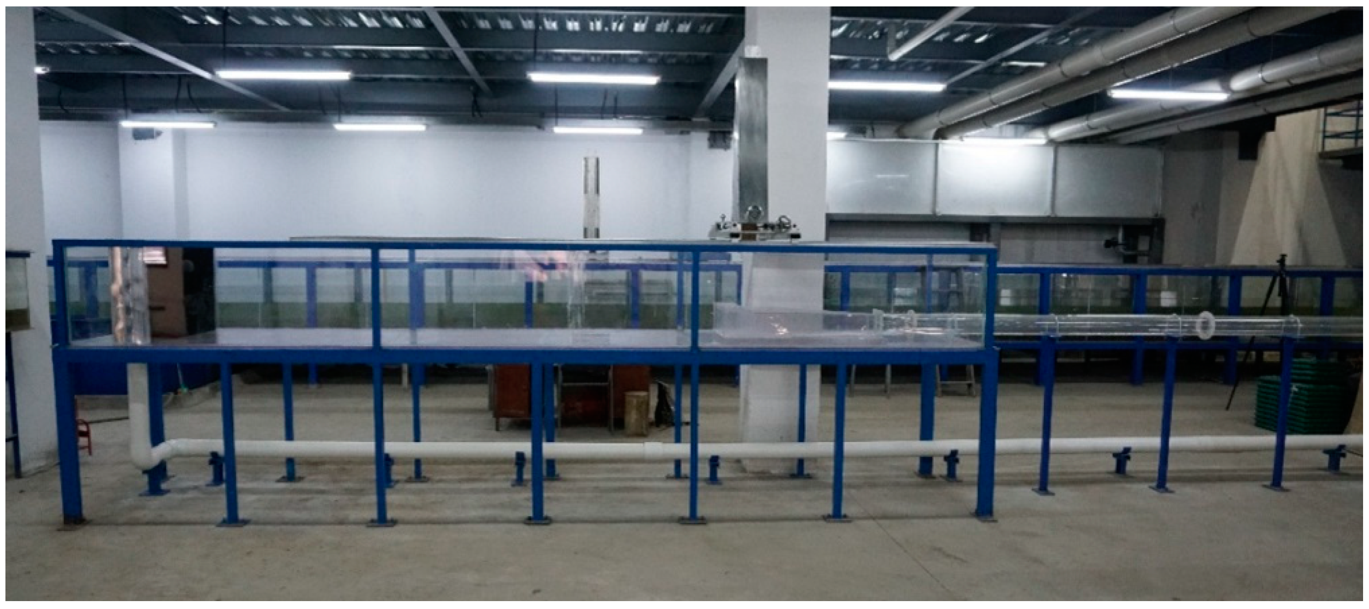
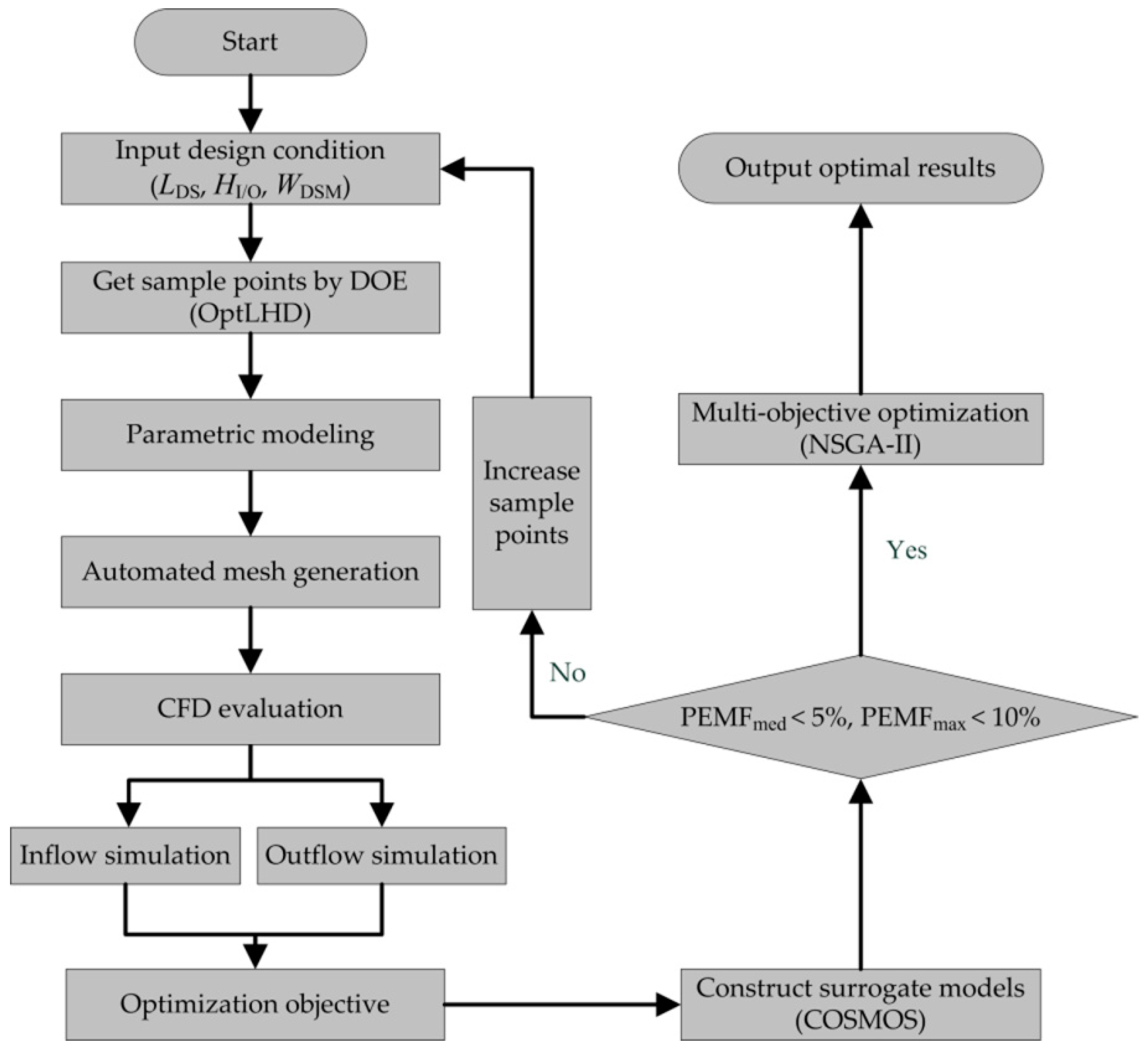
In this article, the CFD numerical simulation and multi-objective surrogate-based optimization strategy method (COSMOS and NSGA-II) were combined to optimize intake shape effectively. The CFD method applied in this paper was validated by a physical experiment carefully designed to meet bidirectional flow requirements for the inlet/outlet. For the purpose of determining a good compromise between the two modes of operation, reasonable weights were defined to better evaluate the overall performance. Then, suitable surrogate models based on COSMOS were utilized to build functions, and NSGA-II was chosen to complete the optimization.
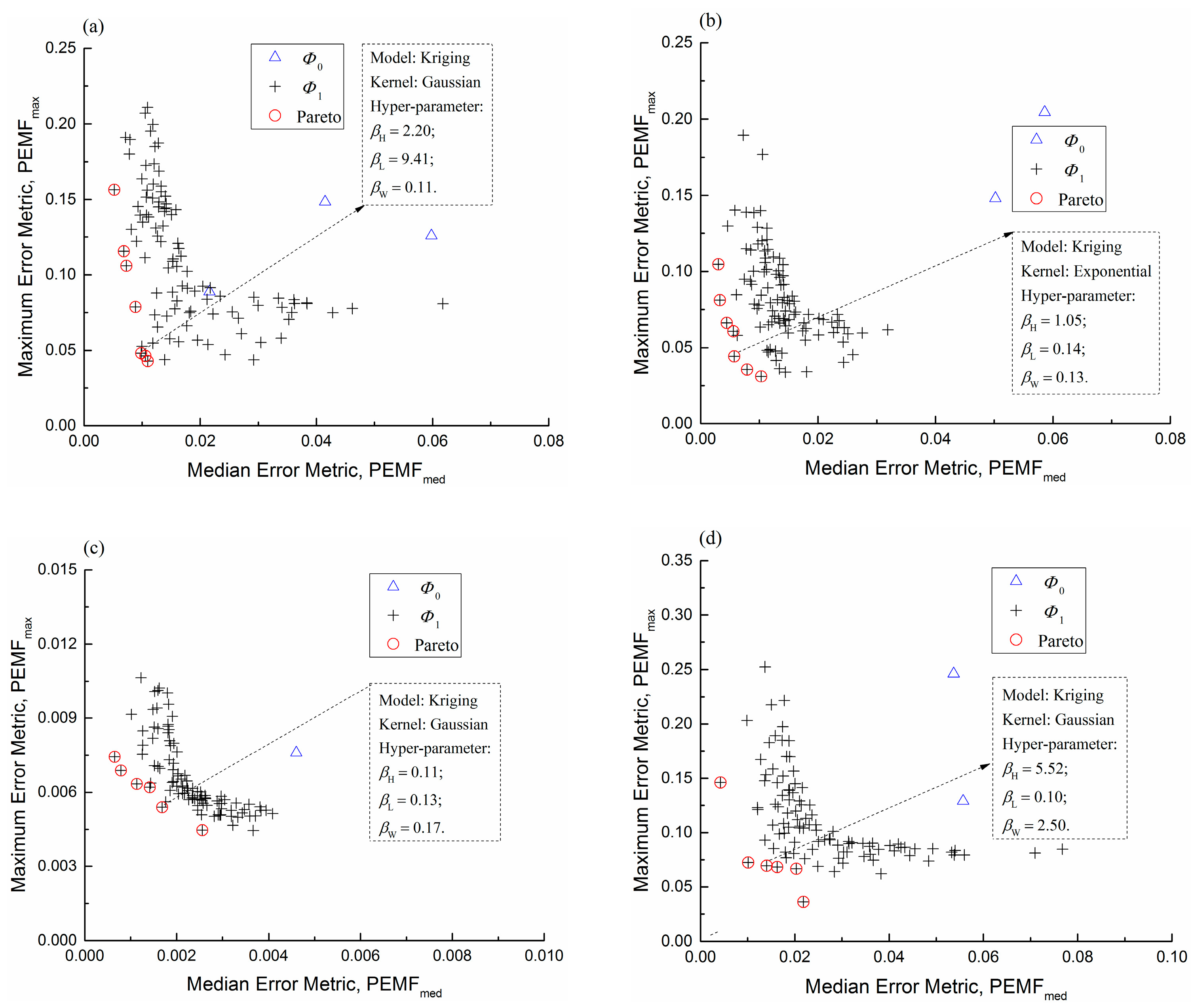
The optimum shape of the diffusion part in a PHES can be achieved automatically through the whole process, including numerical model building, CFD simulation, optimal surrogate model selection, and multi-objective optimization strategy. There were 60 sampling points generated by the OLHS employed to establish suitable surrogate models based on COSMOS, while the PEMF method was applied to estimate errors. The results indicate that the Kriging with a Gaussian kernel is best for the overall head loss coefficient and the shape parameter βH = 2.20, βL = 9.41, βW = 0.11; the best configuration of the overall velocity distribution coefficient is the Kriging model with an Exponential kernel and βH = 1.05, βL = 0.14, βW = 0.13.
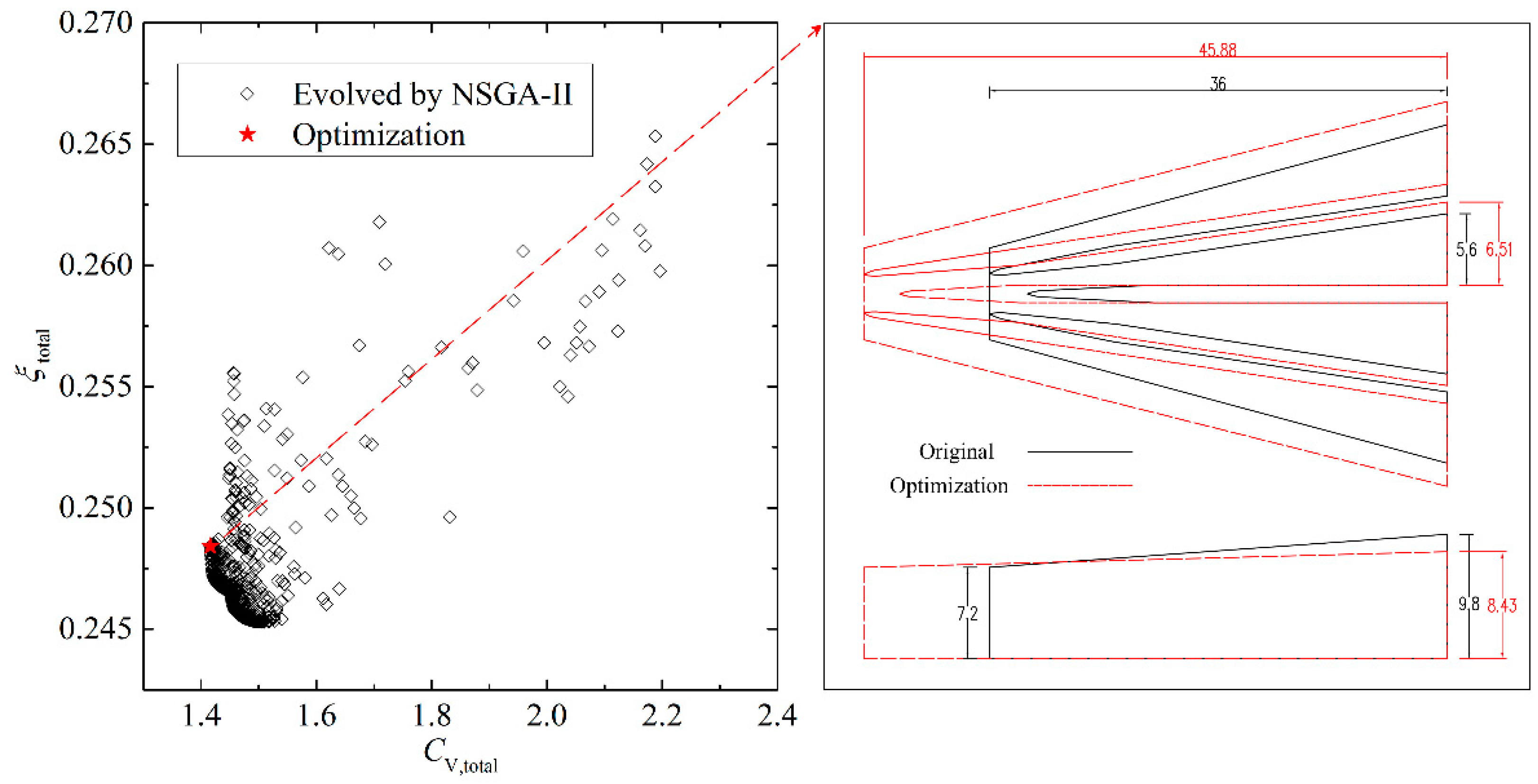
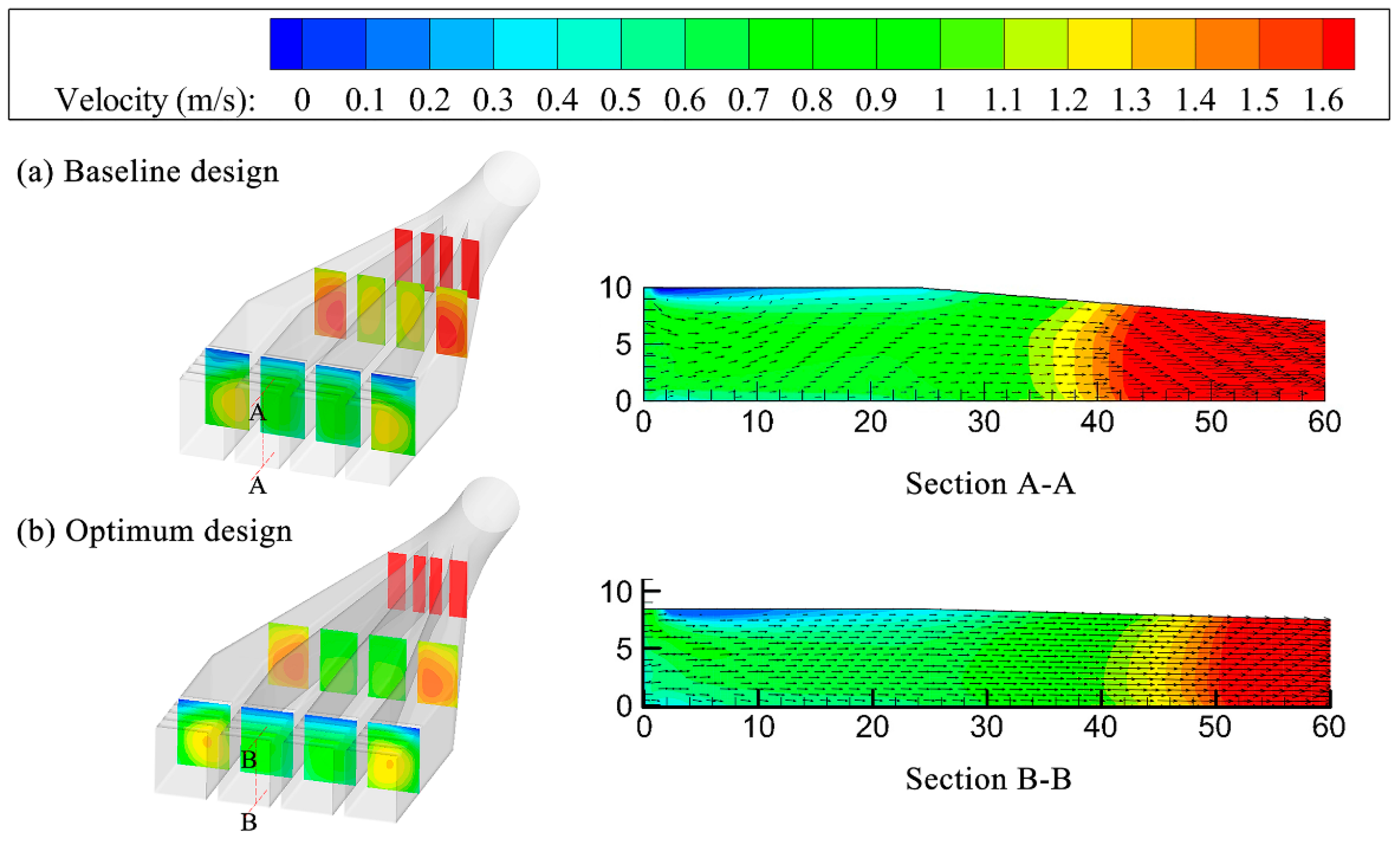
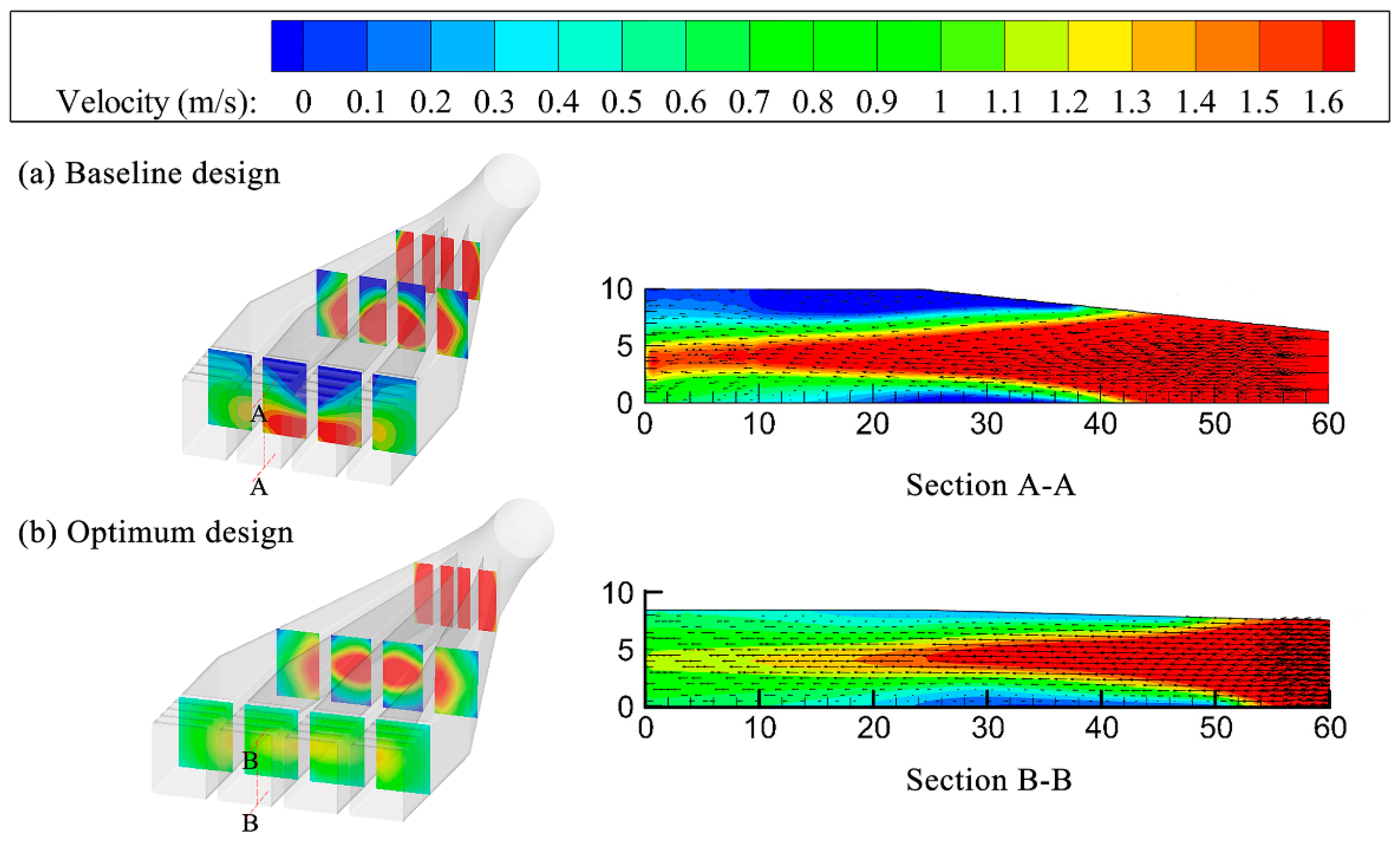
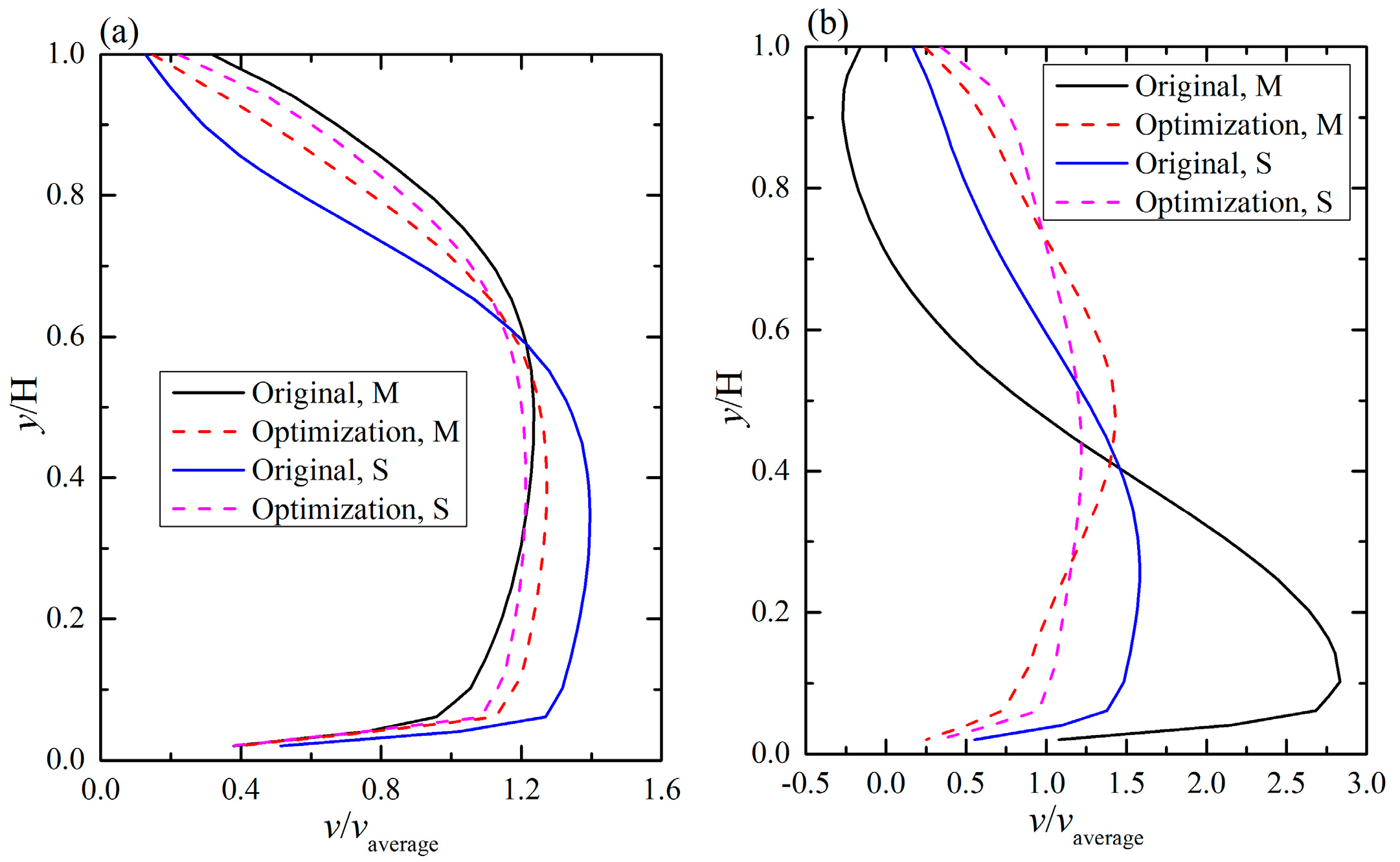
Finally, the NSGA-II algorithm was applied to generate Pareto optimal results, and the final optimal point was selected from the Pareto set through the TOPSIS decision making method. The optimization results show that compared with the original shape the overall head loss coefficient decreases by 6.42% and the overall velocity distribution coefficient decreases by 40.28%. This study demonstrates this new optimization process is a good choice for inlet/outlet engineering designers.

Author Contributions

Conceptualization, X.G. and B.S.; methodology, H.Z. (Hongtao Zhu) and Y.T.; software, H.Z. (Han Zhang) and Z.Q.; validation, Z.Q.; formal analysis, H.Z. (Han Zhang); investigation, H.Z. (Hongtao Zhu) and Y.T.; data curation, Z.Q.; writing—original draft preparation, H.Z. (Hongtao Zhu) and Y.T.; writing—review and editing, H.Z. (Hongtao Zhu) and B.S.; visualization, Z.Q.; supervision, X.G. and B.S.

Funding

This research was funded by the Science Fund for Creative Research Group of the National Natural Science Foundation of China (51621092), the National Natural Science Foundation of China (51279125) and Tianjin Municipal Natural Science Foundation (15JCYBJC22600).

Conflicts of Interest

The authors declare no conflict of interest.

References

  1. Frosina, E.; Buono, D.; Senatore, A. A Performance Prediction Method for Pumps as Turbines (PAT) Using a Computational Fluid Dynamics (CFD) Modeling Approach. Energies 2017, 10, 103. [Google Scholar] [CrossRef]
  2. Itsukushima, R.; Ikematsu, S.; Nakano, M.; Takagi, M.; Shimatani, Y. Optimal structure of grated bottom intakes designed for small hydroelectric power generation. J. Renew. Sustain. Energy 2016, 8, 034501. [Google Scholar] [CrossRef]
  3. Kolekar, N.; Banerjee, A. A coupled hydro-structural design optimization for hydrokinetic turbines. J. Renew. Sustain. Energy 2013, 5, 053146. [Google Scholar] [CrossRef]
  4. Li, D.; Gong, R.; Wang, H.; Wei, X.; Liu, Z.; Qin, D. Numerical investigation on transient flow of a high head low specific speed pump-turbine in pump mode. J. Renew. Sustain. Energy 2015, 7, 063111. [Google Scholar] [CrossRef]
  5. Dong, W.; Li, Y.; Xiang, J. Optimal Sizing of a Stand-Alone Hybrid Power System Based on Battery/Hydrogen with an Improved Ant Colony Optimization. Energies 2016, 9, 785. [Google Scholar] [CrossRef]
  6. Singh, A.; Sevda, S.; Abu Reesh, I.; Vanbroekhoven, K.; Rathore, D.; Pant, D. Biohydrogen Production from Lignocellulosic Biomass: Technology and Sustainability. Energies 2015, 8, 13062–13080. [Google Scholar] [CrossRef]
  7. Belabes, B.; Youcefi, A.; Paraschivoiu, M. Numerical investigation of Savonius wind turbine farms. J. Renew. Sustain. Energy 2016, 8, 053302. [Google Scholar] [CrossRef]
  8. Gosselin, R.; Dumas, G.; Boudreau, M. Parametric study of H-Darrieus vertical-axis turbines using CFD simulations. J. Renew. Sustain. Energy 2016, 8, 053301. [Google Scholar] [CrossRef]
  9. Shen, X.; Avital, E.; Paul, G.; Rezaienia, M.A.; Wen, P.; Korakianitis, T. Experimental study of surface curvature effects on aerodynamic performance of a low Reynolds number airfoil for use in small wind turbines. J. Renew. Sustain. Energy 2016, 8, 053303. [Google Scholar] [CrossRef]
  10. Kumar, A.; Kim, M.-H. Thermal Hydraulic Performance in a Solar Air Heater Channel with Multi V-Type Perforated Baffles. Energies 2016, 9, 564. [Google Scholar] [CrossRef]
  11. Katsaprakakis, D.A.; Christakis, D.G.; Pavlopoylos, K.; Stamataki, S.; Dimitrelou, I.; Stefanakis, I.; Spanos, P. Introduction of a wind powered pumped storage system in the isolated insular power system of Karpathos–Kasos. Appl. Energy 2012, 97, 38–48. [Google Scholar] [CrossRef]
  12. Kocaman, A.S.; Modi, V. Value of pumped hydro storage in a hybrid energy generation and allocation system. Appl. Energy 2017, 205, 1202–1215. [Google Scholar] [CrossRef]
  13. Müller, M.; De Cesare, G.; Schleiss, A.J. Flow field in a reservoir subject to pumped-storage operation—In situ measurement and numerical modeling. J. Appl. Water Eng. Res. 2016, 6, 109–124. [Google Scholar] [CrossRef]
  14. Bermudez, M.; Cea, L.; Puertas, J.; Conde, A.; Martin, A.; Baztan, J. Hydraulic model study of the intake-outlet of a pumped-storage hydropower plant. Eng. Appl. Comput. Fluid Mech. 2017, 11, 483–495. [Google Scholar] [CrossRef]
  15. Cai, F.; Hu, M.; Zhang, Z. Study on guide piers in frank inlet-outlet with double flow directions. J. Hohai Univ. 2000, 28, 74–77. [Google Scholar]
  16. Gao, X.; Wang, Z. The Hydraulic Characteristics at Vertical Pipe Intake of Xilongchi Pumped Storage Plant. J. Hydroelectr. Eng. 2002, 1, 52–60. [Google Scholar]
  17. Sun, S.; Liu, H.; Li, Z.; Sun, C. Study on velocity distribution behind the trashrack in lateral intake/outlet of pumped storage power station. Shuili Xuebao 2007, 38, 1329–1335. [Google Scholar]
  18. Ye, F.; Gao, X. Numerical simulations of the hydraulic characteristics of side inlet/outlets. J. Hydrodyn. Ser. B 2011, 23, 48–54. [Google Scholar] [CrossRef]
  19. Gao, X.; Li, Y.; Tian, Y.; Sun, B. Flow distribution in side intake/outlet tunnel of pumped storage power stations. J. Hydroelectr. Eng. 2016, 35, 87–94. [Google Scholar]
  20. Ansoni, J.L.; Seleghim, P. Optimal industrial reactor design: Development of a multiobjective optimization method based on a posteriori performance parameters calculated from CFD flow solutions. Adv. Eng. Softw. 2016, 91, 23–35. [Google Scholar] [CrossRef]
  21. Ding, Y.; Zhang, X. An optimal design method of swept blades for HAWTs. J. Renew. Sustain. Energy 2016, 8, 043303. [Google Scholar] [CrossRef]
  22. Gao, Q.; Cai, X.; Zhu, J.; Guo, X. Multi-objective optimization and fuzzy evaluation of a horizontal axis wind turbine composite blade. J. Renew. Sustain. Energy 2015, 7, 063109. [Google Scholar] [CrossRef]
  23. Lopez, N.; Mara, B.; Mercado, B.; Mercado, L.; Pascual, M.; Promentilla, M.A. Design of modified Magnus wind rotors using computational fluid dynamics simulation and multi-response optimization. J. Renew. Sustain. Energy 2015, 7, 063135. [Google Scholar] [CrossRef]
  24. Jiang, Y.T.; Lin, H.F.; Yue, G.Q.; Zheng, Q.; Xu, X.L. Aero-thermal optimization on multi-rows film cooling of a realistic marine high pressure turbine vane. Appl. Therm. Eng. 2017, 111, 537–549. [Google Scholar] [CrossRef]
  25. Elsayed, K.; Lacor, C. CFD modeling and multi-objective optimization of cyclone geometry using desirability function, artificial neural networks and genetic algorithms. Appl. Math. Model. 2013, 37, 5680–5704. [Google Scholar] [CrossRef]
  26. Yang, Y.T.; Tang, H.W.; Ding, W.P. Optimization design of micro-channel heat sink using nanofluid by numerical simulation coupled with genetic algorithm. Int. Commun. Heat Mass Transf. 2016, 72, 29–38. [Google Scholar] [CrossRef]
  27. Sun, W.Q.; Cheng, W. Finite element model updating of honeycomb sandwich plates using a response surface model and global optimization technique. Struct. Multidiscip. Optim. 2016, 55, 121–139. [Google Scholar] [CrossRef]
  28. Gan, W.B.; Zhang, X.C. Design optimization of a three-dimensional diffusing S-duct using a modified SST turbulent model. Aerosp. Sci. Technol. 2017, 63, 63–72. [Google Scholar] [CrossRef]
  29. Naseri, S.; Tatar, A.; Shokrollahi, A. Development of an accurate method to prognosticate choke flow coefficients for natural gas flow through nozzle and orifice type chokes. Flow Meas. Instrum. 2016, 48, 1–7. [Google Scholar] [CrossRef]
  30. An, Z.; Zhounian, L.; Peng, W.; Linlin, C.; Dazhuan, W. Multi-objective optimization of a low specific speed centrifugal pump using an evolutionary algorithm. Eng. Optim. 2015, 48, 1251–1274. [Google Scholar] [CrossRef]
  31. Yin, H.; Fang, H.; Wen, G.; Wang, Q.; Xiao, Y. An adaptive RBF-based multi-objective optimization method for crashworthiness design of functionally graded multi-cell tube. Struct. Multidiscip. Optim. 2015, 53, 129–144. [Google Scholar] [CrossRef]
  32. Lotfan, S.; Ghiasi, R.A.; Fallah, M.; Sadeghi, M.H. ANN-based modeling and reducing dual-fuel engine’s challenging emissions by multi-objective evolutionary algorithm NSGA-II. Appl. Energy 2016, 175, 91–99. [Google Scholar] [CrossRef]
  33. Liu, C.; Bu, W.; Xu, D. Multi-objective shape optimization of a plate-fin heat exchanger using CFD and multi-objective genetic algorithm. Int. J. Heat Mass Transf. 2017, 111, 65–82. [Google Scholar] [CrossRef]
  34. Jakumeit, J.; Herdy, M.; Nitsche, M. Parameter optimization of the sheet metal forming process using an iterative parallel Kriging algorithm. Struct. Multidiscip. Optim. 2005, 29, 498–507. [Google Scholar] [CrossRef]
  35. Zhang, Y.; Hu, S.; Wu, J.; Zhang, Y.; Chen, L. Multi-objective optimization of double suction centrifugal pump using Kriging metamodels. Adv. Eng. Softw. 2014, 74, 16–26. [Google Scholar] [CrossRef]
  36. Mehmani, A.; Chowdhury, S.; Meinrenken, C.; Messac, A. Concurrent surrogate model selection (COSMOS): Optimizing model type, kernel function, and hyper-parameters. Struct. Multidiscip. Optim. 2017, 57, 1093–1114. [Google Scholar] [CrossRef]
  37. Gao, X.; Tian, Y.; Sun, B. Shape optimization of bi-directional flow passage components based on a genetic algorithm and computational fluid dynamics. Eng. Optim. 2017, 50, 1287–1303. [Google Scholar] [CrossRef]
  38. Gao, X.; Tian, Y.; Sun, B. Multi-objective optimization design of bidirectional flow passage components using RSM and NSGA II: A case study of inlet/outlet diffusion segment in pumped storage power station. Renew. Energy 2018, 115, 999–1013. [Google Scholar] [CrossRef]
  39. Design Guide for Pumped Storage Power Station (DL/T 5208-2005); China Electric Power Press: Beijing, China, 2005.
  40. Johnson, P.L. HydroPower Intake Design Considerations. J. Hydraul. Eng. 1988, 114, 651–661. [Google Scholar] [CrossRef]
  41. Sell, L.E. Hydroelectric Power Plant Trashrack Design. J. Power Div. 1971, 97, 115–121. [Google Scholar]
  42. Lei, T.; Shan, Z.B.; Liang, C.S.; Chuan, W.Y.; Bin, W.B. Numerical simulation of unsteady cavitation flow in a centrifugal pump at off-design conditions. Proc. Inst. Mech. Eng. Part C J. Mech. Eng. Sci. 2013, 228, 1994–2006. [Google Scholar] [CrossRef]
  43. Tan, L.; Zhu, B.; Wang, Y.; Cao, S.; Gui, S. Numerical study on characteristics of unsteady flow in a centrifugal pump volute at partial load condition. Eng. Comput. 2015, 32, 1549–1566. [Google Scholar] [CrossRef]
  44. Liu, Y.; Tan, L.; Hao, Y.; Xu, Y. Energy Performance and Flow Patterns of a Mixed-Flow Pump with Different Tip Clearance Sizes. Energies 2017, 10, 191. [Google Scholar] [CrossRef]
  45. Fluent. User’s and Theory Guide; ANSYS, Inc.: Canonsburg, PA, USA, 2015. [Google Scholar]
  46. Shih, T.-H.; Liou, W.W.; Shabbir, A.; Yang, Z.; Zhu, J. A new k-ϵ eddy viscosity model for high reynolds number turbulent flows. Comput. Fluids 1995, 24, 227–238. [Google Scholar] [CrossRef]
  47. Sun, H.; Shin, H.; Lee, S. Analysis and optimization of aerodynamic noise in a centrifugal compressor. J. Sound Vib. 2006, 289, 999–1018. [Google Scholar] [CrossRef]
  48. Khalfallah, S.; Ghenaiet, A. Shape optimization of a centrifugal compressor impeller. In Proceedings of the Institution of Mechanical Engineers, 8th International Conference on Compressors and their Systems, London, UK, 9–10 September 2013; Woodhead Publishing Limited: Cambridge, UK, 2013. [Google Scholar]
  49. Zhou, C.; Yang, C.; Zhang, X.; Wang, C. A simulation-based two-step method for optimal thermal design of multiple compartments. Appl. Therm. Eng. 2017, 122, 535–545. [Google Scholar] [CrossRef]
  50. Brar, L.S.; Elsayed, K. Analysis and optimization of multi-inlet gas cyclones using large eddy simulation and artificial neural network. Powder Technol. 2017, 311, 465–483. [Google Scholar] [CrossRef]
  51. Li, Z.; Liu, Y. Blade-end treatment for axial compressors based on optimization method. Energy 2017, 126, 217–230. [Google Scholar] [CrossRef]
  52. Zhang, M.; Gou, W.; Li, L.; Yang, F.; Yue, Z. Multidisciplinary design and multi-objective optimization on guide fins of twin-web disk using Kriging surrogate model. Struct. Multidiscip. Optim. 2017, 55, 361–373. [Google Scholar] [CrossRef]
  53. Singh, P.; Couckuyt, I.; Elsayed, K.; Deschrijver, D.; Dhaene, T. Shape optimization of a cyclone separator using multi-objective surrogate-based optimization. Appl. Math. Model. 2016, 40, 4248–4259. [Google Scholar] [CrossRef]
  54. Wang, B.; Li, T.; Ge, L.; Ogawa, H. Optimization of combustion chamber geometry for natural gas engines with diesel micro-pilot-induced ignition. Energy Convers. Manag. 2016, 122, 552–563. [Google Scholar] [CrossRef]
  55. Halder, P.; Samad, A.; Thevenin, D. Improved design of a Wells turbine for higher operating range. Renew. Energy 2017, 106, 122–134. [Google Scholar] [CrossRef]
  56. Martin, J.D.; Simpson, T.W. Use of Kriging Models to Approximate Deterministic Computer Models. Aiaa J. 2005, 43, 853–863. [Google Scholar] [CrossRef]
  57. Viana, F.A.C.; Haftka, R.T.; Steffen, V. Multiple surrogates: How cross-validation errors can help us to obtain the best predictor. Struct. Multidiscip. Optim. 2009, 39, 439–457. [Google Scholar] [CrossRef]
  58. Gorissen, D.; Couckuyt, I.; Demeester, P.; Dhaene, T.; Crombecq, K. A Surrogate Modeling and Adaptive Sampling Toolbox for Computer Based Design. J. Mach. Learn. Res. 2010, 11, 2051–2055. [Google Scholar]
  59. Mehmani, A.; Chowdhury, S.; Messac, A. Predictive quantification of surrogate model fidelity based on modal variations with sample density. Struct. Multidiscip. Optim. 2015, 52, 353–373. [Google Scholar] [CrossRef]
  60. Lophaven, S.N.; Nielsen, H.B.; Sondergaard, J. DACE—A MATLAB Kriging Toolbox—Version 2.0, Informatics and Mathematical Modeling; Technical University of Denmark: Lyngby, Denmark, 2002. [Google Scholar]
  61. Deb, K.; Pratap, A.; Agarwal, S.; Meyarivan, T. A fast and elitist multiobjective genetic algorithm: NSGA-II. IEEE Trans. Evol. Comput. 2002, 6, 182–197. [Google Scholar] [CrossRef]
  62. Deb, K.; Agrawal, R.B. Simulated Binary Crossover for Continuous Search Space. Complex Syst. 1994, 9, 115–148. [Google Scholar]
  63. Deb, K.; Goyal, M. A Combined Genetic Adaptive Search (GeneAS) for Engineering Design. Comput. Sci. Inform. 1996, 26, 30–45. [Google Scholar]
  64. Hwang, C.L.; Yoon, K.P. Multiple Attribute Decision Making—Methods and Applications: A State-of-the-Art Survey; Springer: Berlin/Heidelberg, Germany, 1981; pp. 11, 269. [Google Scholar]
Figure 1. General structure of the lateral intake-outlet.
Processes 07 00204 g001
Figure 2. Basic parameters for the diffusion part.
Processes 07 00204 g002
Figure 3. Grids generation for the computational domain: (a) grids on the boundary; (b) grids at the orifice cross-section, and (c) grids on the orifice horizontal section.
Processes 07 00204 g003
Figure 4. The Distribution of y+ values for the inlet/outlet: (a) the inflow condition; (b) the outflow condition.
Processes 07 00204 g004
Figure 5. The experimental setup of the inlet/outlet.
Processes 07 00204 g005
Figure 6. The side layout plan for the experimental system of the inlet/outlet.
Processes 07 00204 g006
Figure 7. Measured lines at the cross-section (x = 10 m).
Processes 07 00204 g007
Figure 8. Validation for the velocity distribution in the inflow condition: (a) middle orifice; (b) side orifice.
Processes 07 00204 g008
Figure 9. Validation for the velocity distribution in the outflow condition: (a) middle orifice; (b) side orifice.
Processes 07 00204 g009
Figure 10. Flow diagram of the multi-objective optimization process.
Processes 07 00204 g010
Figure 11. Surrogate model selection of hydraulic performance indices: (a) ξ; (b) CV; (c) CQ,in; (d) CQ, out.
Processes 07 00204 g011
Figure 12. The process of objectives evolved through NSGA-II (dimensions in m).
Processes 07 00204 g012
Figure 13. The comparison of inflow velocity distribution between the baseline and optimum design.
Processes 07 00204 g013
Figure 14. The comparison of outflow velocity distribution between the baseline and optimum design.
Processes 07 00204 g014
Figure 15. Velocity profiles at the orifice cross-section: (a) inflow; (b) outflow.
Processes 07 00204 g015
Table 1. Design parameters and constraints.
ItemSymbolRange
Design parametersLDS34–46 m
HI/O8–11 m
WDSM1.5–1.7 m
Constraintsη25–45°
θ1–5°
CQ,in, CQ,out<10%
Table 2. Boundary conditions applied in the inlet/outlet CFD simulation.
Operation ModesParametersNotesValues
OutflowInletThe inlet of the pipe was defined as the velocity inlet.vd = 3.738 m/s
OutletThe reservoir boundary was defined as the pressure outlet.Relative pressure: 0 Pa
InflowInletThe reservoir boundary was defined as the pressure inlet.Relative pressure: 0 Pa
OutletThe inlet of the pipe was defined as the velocity outlet.vd = 4.376 m/s
Table 3. A list of shape optimization investigated using surrogate models in recent years.
AuthorDesign ParameterObjective FunctionSampling PointsSurrogate ModelOptimization Algorithm
Zhou et al. [49]3230RSMNSGA-II
Jiang et al. [24]102150RSMNSGA-II
Yang et al. [26]3120RSMGA
Brar et al. [50]3330RBFNSGA-II
Li et al. [51]5160RBFGA
Zhang et al. [52]162262KrigingNSGA-II
Liu et al. [33]4250KrigingNSGA-II
Singh et al. [53]7271RBF, KrigingNSGA-II
Wang et al. [54]7280RSM, RBF, KrigingNSGA-II
Halder et al. [55]2116RSM, RBF, KrigingGA
Table 4. Parameters of surrogate model candidates.
Model TypeKernel FunctionHyper-ParameterLower/Upper Bounds
Response surface methodology---
Radial Basis FunctionLinear--
Cubic--
GaussianShape parameter, α0.1 < α < 3
MultiquadricShape parameter, α0.1< α < 3
KrigingLinearCorrelation parameter, β0.1 < β < 20
ExponentialCorrelation parameter, β0.1 < β < 20
GaussianCorrelation parameter, β0.1 < β < 20
SphericalCorrelation parameter, β0.1 < β < 20
Table 5. The parameters for the optimization process.
ParameterValues
Population size (even value)100
Number of Generations100
Crossover Probability0.9
Crossover Distribution Index10.0
Mutation Distribution Index20.0
Table 6. Optimal surrogate model configurations and their Predictive Estimation of Model Fidelity (PEMF) errors.
IndexOptimal Surrogate Model ConfigurationPEMF Error
Model TypeKernel FunctionHyper-ParameterMedianMax
ξtotalKrigingGaussianβH = 2.20, βL = 9.41, βW = 0.110.00980.0481
CV,totalKrigingExponentialβH = 1.05, βL = 0.14, βW = 0.130.00570.0443
C Q , in KrigingGaussianβH = 0.11, βL = 0.13, βW = 0.170.00170.0054
C Q , out KrigingGaussianβH = 5.52, βL = 0.10, βW = 2.500.01410.0695
Table 7. The comparison of parameters between baseline case and optimum case.
CaseDesign VariablesObjectivesVariation (%)
HI/O (m)LDS (m)WDSM (m)ξtotalCV,totalΔξtotalΔCV,total
Baseline9.80036.0001.5800.2652.371−6.42−40.28
Optimum8.43245.8751.5130.2481.416

