Optimal Operating Schedule for Energy Storage System: Focusing on Efficient Energy Management for Microgrid

Abstract

A microgrid is a group of many small-scale distributed energy resources, such as solar/wind energy sources, diesel generators, energy storage units, and electric loads. As a small-scale power grid, it can be operated independently or within an existing power grid(s). The microgrid energy management system is a system that controls these components to achieve optimized operation in terms of price by reducing costs and maximizing efficiency in energy consumption. A post-Industry-4.0 consumer requires an optimal design and control of energy storage based on a demand forecast, using big data to stably supply clean, new, and renewable energy when necessary while maintaining a consistent level of quality. Thus, this study focused on software technology through which an optimized operation schedule for energy storage in a microgrid is derived. This energy storage operation schedule minimizes the costs involved in electricity use. For this, an optimization technique is used that sets an objective function representing the information and costs pertaining to electricity use, while minimizing its value by using Mixed Integer Linear Programming or a Genetic Algorithm. The main feature of the software is that an optimal operation schedule derivation function has been implemented with MATLAB for the following circumstances: when the basic operation rules are applied, when operating with another grid, when the external operating conditions are applied, and when the internal operating conditions are applied.

1. Introduction

A microgrid is a small-scale power grid consisting of a series of small-scale distributed energy resources (DER) and loads, such as solar/wind energy sources, diesel generators, and energy storage, operating independently or within an existing power grid(s) [1]. The microgrid energy management system is a system that controls these components to achieve optimized operation in terms of price by reducing costs and maximizing efficiency in energy consumption. In the era of post-Industry-4.0, optimal design and control of energy storage based on an accurate demand forecast using big data is essential to stably supply clean, new, and renewable energy when necessary, while maintaining a consistent level of quality, whereas energy producers are required to efficiently and stably manage integrated energy resources produced from new and renewable energy production facilities, and existing nuclear, thermal, co-generation, and gas-turbine power plants.

At the same time, for energy consumers, an accurate power demand forecast that takes into account various types of power consumption patterns depending on their housings, and the inconvenience associated with demand response projects for peak-load control is required. Thus, energy management software that efficiently schedules energy storage by effectively carrying out the charging/discharging process repeatedly between the process of energy production and consumption is needed. So, this study focuses on the operation and control of a microgrid in a zero-energy smart city, dealing in particular with software technology that derives an optimal operation schedule for energy storage in a microgrid [2].

From an economic standpoint, some of the most important elements are the production, management, and consumption of energy or energy products. These are associated with many other critical social elements such as food production, water consumption, manufacturing, resource management, security, and the environment. Currently, process system engineering can be used to solve many important problems associated with energy systems and mitigate their impact worldwide [3]. Additionally, the advent of the Fourth Industrial Revolution has been widely discussed over the past few years, and current electric power supply systems are central to its realization. An undisruptive power supply is essential for motor function at nuclear, thermal, and wind power stations, as well as motors in manufacturing factories. If power is disrupted, an excitation system will kick in to prevent power failure before accidents or damage can occur [4].

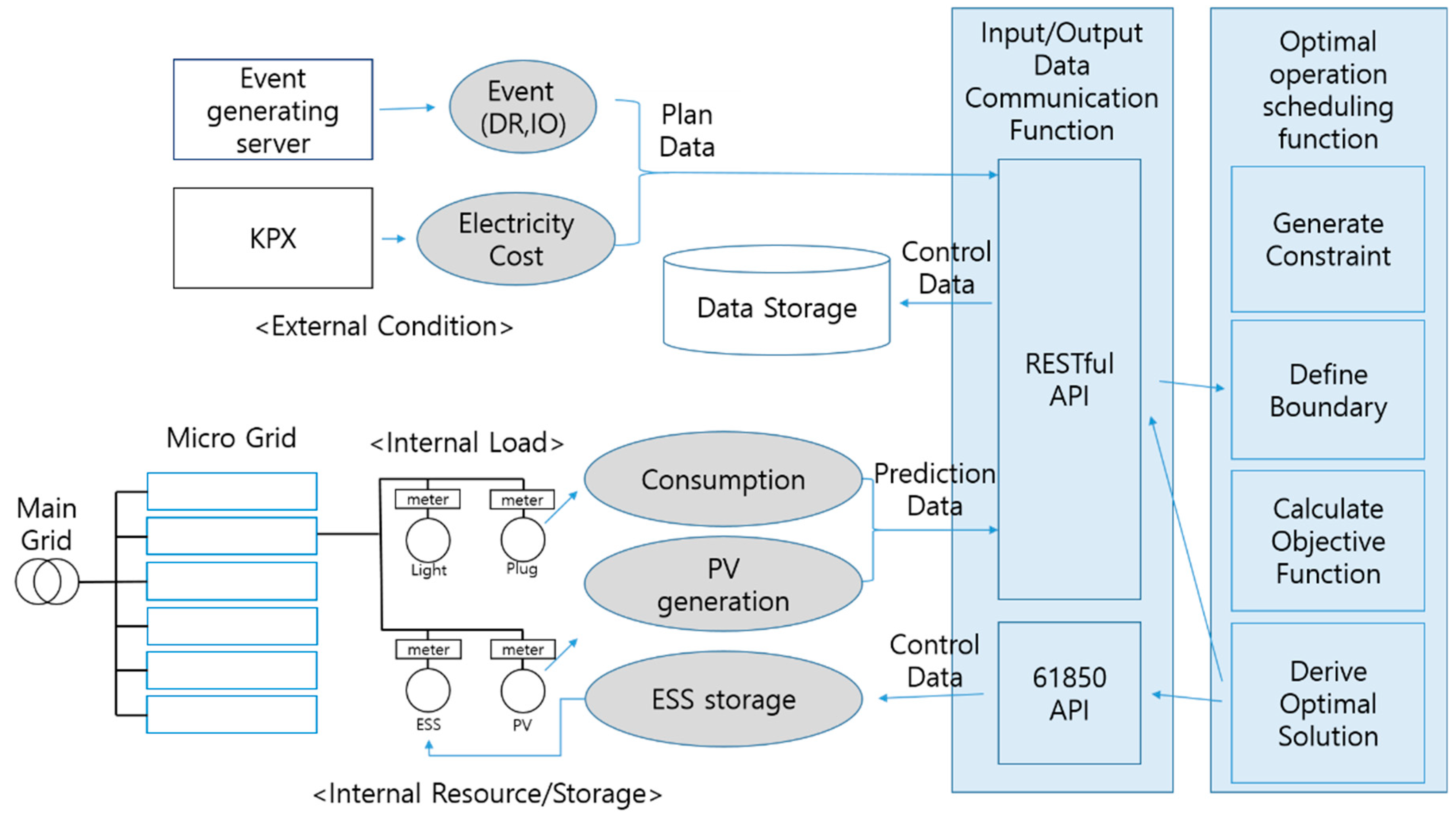
The operation flow diagram of microgrid energy management system software is presented below, and the software proposed in this study specifically focuses on the data input/output function and the optimal operation scheduling function to derive an optimal schedule that maximizes the economic effects of the microgrid by collecting the basic operating rules, expected supply and demand data of power consumption/production resources, power supply unit cost information, external special event/action information, and internal control settings.

Figure 1 shows the operation flow diagram of a microgrid energy management system. An optimization technique is used in the process of deriving an operating schedule. After setting an objective function, representing the information and costs pertaining to electricity use, its value is minimized using mixed integer linear programming or a genetic algorithm.

The main feature of the software proposed in this study is that an optimal operation schedule derivation function has been implemented with MATLAB (9.4.0.796201, MathWorks, Natick, MA, USA, 2018) and Python (3.6.6, Python Software Foundation, Wilmington, DE, USA, 2018) for the following circumstances: when the basic operation rules are applied, when operating with another grid, when the external operating conditions are applied, and when the internal operating conditions are applied. One notable feature of the software is that the next best schedule can be derived by adding an additional value to the conditional expression when applying an external condition, even if it does not satisfy some of the operating conditions.

The goal of this research is to derive an optimal operating schedule based on the appropriate use of input/output data; that is, outputting the optimal operating schedule for the energy storage system (ESS) which guarantees economic feasibility by entering input values such as Korean operating rules, expected supply-demand data of power consumption and generation resources, power supply unit price, external particular operating events, and internal control setpoints.

2. Related Study

Deriving an operating schedule is one of the most important elements of the energy management system on which numerous studies have been conducted. In Li et al. [5], the design and implementation of a green home service for the management of residential energy was discussed, whereas in Al-Ali et al. [6], the design and implementation of a smart home using new and renewable energy (solar) along with energy storage was discussed together with its test run. Zhang et al. [7] considered an optimization algorithm, which is to be used for the home in a smart grid. Rodriguez and Braun [8] compared the operation of a microgrid applied with or without an optimization algorithm, whereas Luna et al. [9] focused on the energy management system of a microgrid with its own power generation system and connected to the existing power grid. In Li et al. [10], issues pertaining to the energy management system of an industrial microgrid operating independently or being connected to the existing power grid are discussed. Arcos-Aviles et al. [11] describe the design of a fuzzy-logic-based energy management system of a microgrid with new and renewable energy resources as well as energy storage, while connected to the existing power grid. A two-hierarchy prediction energy management system is discussed in Ju et al. [12]. Research studies have also been conducted on operating schedule derivation. In Gamarra and Guerrero [13] and Kim and Kinoshita [14], the minimization of operating costs using a basic model was discussed, whereas Mohamed and Koivo [15,16] considered a system model of a microgrid with battery storage and online management, aimed to minimize costs while satisfying demand, considering individual situations in which there is wind, diesel, or a solar generator, as well as fuel cells and battery storage.

Parisio and Gilelmo [17] discussed the management of a microgrid using model predictive control. The load in the calculation was reduced while improving the calculation results using mixed integer linear programming. Malysz et al. [18] focused on the minimization of operating costs of an energy storage device operating together with a grid. The future power usage and the power generation based on new and renewable energy were forecasted by applying mixed integer linear programming.

Meanwhile, in Hori et al. [19], the introduction of an additional control to respond to expected errors was discussed, whereas Shi et al. [20] focused on managing distributed energy. Finally, Zhang et al. [21] explained an operation model based on model predictive control and its uncertainties.

Meanwhile, Advanced Metering Infrastructure (AMI) is a form that took the automatic meter reading, which is a uni-directional meter, one step forward, and it refers to the infrastructure for the implementation of various optional or additional services through bi-directional data communications between the power company and the consumers. It is also a means of information provision for mutual awareness between them. Various types of decentralized power supply systems and intelligent power distribution systems are included, and it supports highly developed time-based tariff systems such as time-of-usage, critical peak pricing, and real-time pricing. Through AMI, it is possible to induce users to participate in an active energy conservation program called the demand response (DR). DR enables basic data generation and power usage through bi-directional communications between meters and the power company, so an infrastructure containing additional services such as load anticipation, load control, and power quality monitoring is possible [22,23,24,25].

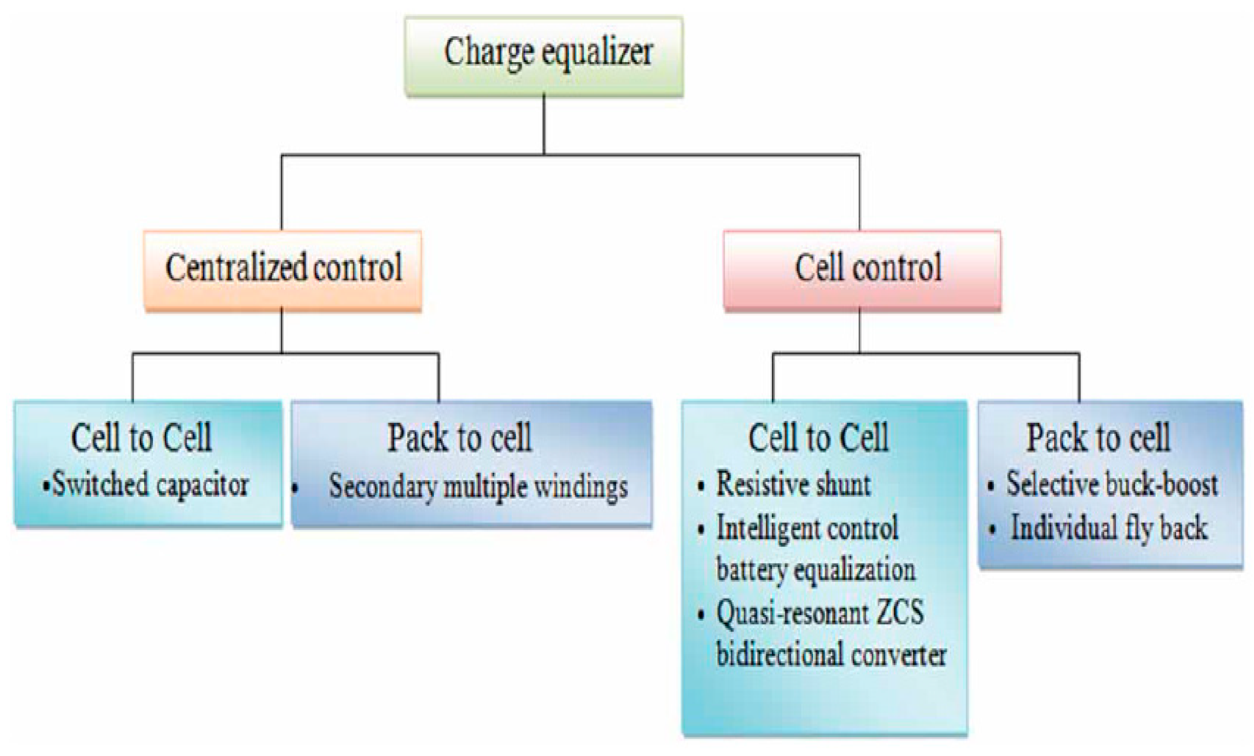
In general, battery management systems developed to focus on the design of switching circuitry so far adopt either the passive charge equalization method or the active charge equalization method. The former is referred to as a dissipative charge equalization since the resistor (dissipative element) linked as a shunt circuit disperses the surplus energy. In contrast, resistors linked in parallel in individual batteries should have the same value. Therefore, powerful batteries with higher State of Charge (SoC) would dissipate much more power across the link than less powerful batteries, which have lower SoC. However, they will all be in balance over time. Not many years ago, multi-winding transformers that equalize charges were introduced, but their major downside was leakage inductance [26,27].

Transistors are usually organized in parallel, whereas the Zener diode breakdown voltage is considered a reference voltage of individual batteries, the voltage level on which the bypass circuit will be activated. Non-dissipative charge equalization, which is another name for active charge equalization, allows active (non-dissipative) elements to transfer energy from one battery to other batteries. The capacitor mounted on a switched capacitor circuit switches its contact form depending on battery power. For example, it switches to the lower-powered battery when the voltage levels are different between two batteries. Although this kind of circuitry is efficient in some situations, one problem is that the energy levels of batteries aligned in a stack will eventually equalize over time through change transfer, even though it may take quite some time to balance out the SOC.

Meanwhile, the switch inductor works similarly to the switched capacitor, but the difference is that a reactor is used to equalize the charge. The resonant equalization performs the charge equalization work between connected batteries through an energy transfer process using resonant circuits composed of L and C components and connected in parallel. However, the major weak point is that the energy transfer can only be achieved between the adjacent batteries [28], and the Direct Current (DC)-to-DC converter circuit seems to be an alternative solution in which the converter is connected to a common bus to conveniently transfer energy from a stronger battery cell to a weak one, regardless of their positions in the stack (Figure 2).

Additionally, this converter is able to consistently check voltage levels and compare them with the reference voltage while charging the batteries. When individual batteries reach the reference voltage, the converter will discontinue charging and separate itself from the battery, transferring the energy to the bus, from which energy will be supplied to a weak battery. The bi-directional DC-to-DC converter is used to transfer energy via the main bus when the discharging process starts. A different design of such a converter topology, consisting of MOS Field-Effect Transistor (MOSFET) switches, was introduced by Hanxin et al. In the design, only the switching circuits of a strong battery and a weak battery are active among the batteries in the stack, so that the energy is not dispersed across all of the switches. Despite such a novel idea, its disadvantages are that its design involves a two-level inverter architecture and its total harmonic distortion tends to be relatively high [26,27,28,29,30,31].

Approaches focusing on optimization were mainly noted in [32,33,34,35,36,37,38,39,40,41] for the above reason [31]. A DC microgrid involving the optimization-oriented Photovoltaic Management System (PMS) was designed to meet the power demand and limit/control the charge current for batteries as well as to establish the wind subsystem as a primary resource in the power system [32,33]. All the PMSs introduced in [34,35,36,37] aim to minimize operating costs, but the Alternating Current (AC) and DC microgrids were considered in [34,35] and [36,37], respectively, whereas the wind/battery-based microgrid was introduced in [38] where the described PMS was to maximize the profit of the power being traded. The battery microgrid was discussed in [39], focusing on minimizing the energy costs for system owners by adopting an optimization-oriented PMS. The AC microgrid system with a similar PMS was proposed in [40], aiming to minimize operating costs or to reduce fuel consumption while also reducing the frequency of the start/stop process of a distributed generator (DG). Even though these PMSs exhibited relatively acceptable performance, prediction errors were not considered in their design, so their feasibility has yet to be studied. Another PMS is being introduced in [41], particularly for grid-connected systems, and it deals with prediction errors in its design.

The hybrid AC/DC microgrid can be considered a novel concept, classifying DC (AC) sources based on DC (AC) loads when the power is transferred between them via a bi-directional converter or inverter [42,43]. Only a few studies have addressed issues involving the power management system of this grid. Liu et al. [44] describes the hybrid AC/DC micro-grid consisting of a AC source and a PV array (DC source). A rule-based scheme was proposed for this grid to flexibly share power between AC and DC microgrids. For the same purpose, [45,46,47] proposed a droop-based controller. The grids are considered separate with their own droop mode that determines the power amount to be exchanged between them by interacting together. At the same time, [48,49] suggest that the power-sharing amount between the grids should be determined by some sort of a rule-based power management system based on the four predefined operating modes. Finally, [50] introduces a particular rule-based PMS for the same microgrids where fifteen operating modes are being applied.

Microgrids can be considered an energy distribution system consisting of DERs including DGs and ESSs as well as loads, and can be operated independently or with another grid(s) [51,52,53]. Current power electronic-based energy technology makes it convenient for the grids to adopt new and renewable energy sources (RES) and efficient ESSs into their systems to operate them efficiently and reliably [54,55]. Despite such benefits, the uncertainties and variability in the energy production process for these energy resources are yet to be solved when actually implementing the grids [56,57]. Deriving a method that can actually establish an optimal operation schedule has been one of the major research goals for power grid researchers whose main target is to develop an uninterrupted power supply system and achieve relevant economic objectives by utilizing it [58]. To avoid any system interruptions or instability, energy management should be performed at a level lower than power and control management levels [52], as the operating schemes on these levels are critical to the operating conditions associated with the system current/voltage, frequency regulation, active/reactive powers, power source transfer, and the provision of additional/optional services [53,59,60,61].

The role of the power management level should be specifically defined in terms of functionality, which is to control the operations involving line limits, power loss, converter/inverter droop, and independent or autonomous operating schemes. Meanwhile, the energy management level needs to guarantee the supply of power resources for a long period of time to optimally balance power generation with the actual demand [62,63,64,65,66,67]. Thus, the microgrid energy management system sets the baseline for the DER or load controller to create an optimal operating condition based on the current state of the grid, economic or technical constraints, and external or environmental requirements [68,69]. The microgrid energy management system tends to abide by short-term operating schedules in which the input parameters and profiles used for forecasting available resources are often determined under uncertain conditions [70,71].

The software technology used to plan the optimal operating schedule for the microgrid energy storage to minimize the operating costs is introduced in this study. An optimization technique that starts by setting an objective function along with relevant data values such as the costs associated with power supply and demand is used for the technology, whereas mixed integer programming or the genetic algorithm is used to minimize the values. This software technology introduces the functions that can be applied to the four different conditions for which an optimal operating schedule will be derived: when the basic operation rules are applied, operating with another grid, when the external operating conditions are applied, and finally when the internal operating conditions are applied. These functions have been implemented with MATLAB because of its efficiency in numerical analysis.

3. Optimal Operating Schedule for Energy Storage System Model

For the optimization technique for deriving an optimal schedule, a mixed integer linear programming and a genetic algorithm were used, and detailed functions included the derivation of an optimal operating schedule when the basic operating rules are applied; operating in conjunction with the grid; external operating conditions are applied; and when internal operating conditions are applied. One of the advantages of these functions is that the next best schedule can be generated by introducing some additional variables into the conditional functions when external operating conditions are applied.

According to Rodriguez and Braun [8], the software being discussed in this study sets the objective function $J$ as follows:

$$\begin{array}{l}J=\Sigma [c_{buy}\left(i\right)p^{c_b}\left(i\right)-c_{sell}\left(i\right)p^{d_s}\left(i\right)-c_{buy}\left(i\right)p^{d_b}\left(i\right)+c_{sell}\left(i\right)p^{c_s}\left(i\right)\\ +0.5\left\{c_{sell}\left(i\right)+c_{buy}\left(i\right)\right\}{p}^{c_u}\left(i\right)-0.5\left\{c_{sell}\left(i\right)+c_{buy}\left(i\right)\right\}{p}^{d_u}\left(i\right)+w_c\left(i\right)\\ +w_d\left(i\right)+\Gamma z_c+\Gamma z_d]dt\end{array}$$

(1)

where $\left(i\right)$ in each item is information for time zone $i$. For instance, $c_{buy}\left(i\right)$ is the purchase price of per unit electric power from a grid in time zone $i$. The explanation for time zone $i$ will not be given in the following sections to speed up the concept.

For example, even though $c_{sell}\left(i\right)$ is ‘the selling price of per unit power to the grid in time zone $i$’, it is simplified as ‘the selling price of per unit power to the grid’. The charging rate of the storage purchased by the grid is given by $p^{c_b}\left(i\right)$, whereas $p^{c_b}\left(i\right)$ is the discharging rate sold to the grid. In addition, $p^{d_b}\left(i\right)$ is the discharging storage rate, which can offset the power volume purchased from the grid. Meanwhile, $p^{c_u}\left(i\right)$ represents the discharging storage rate associated with uncertainty. And finally, $w_c\left(i\right)$, $w_d\left(i\right)$, $\Gamma$, $z_c$, and $z_d$ are variables associated with uncertainty but do not have any physical meaning.

The expected values of the load, power generation, and per unit electric power rate are used as constraints. In short, assuming that the future (24 h, for example) values of the elements affecting power use can be determined now, a schedule for future energy storage use that minimizes the value of the objective function can be prepared based on those values, deriving a schedule for future energy storage use.

Prior to inducing the constraints, some of the variables whose substitute values may change depending on the situation should be explained:

$$P_{max}^{d_b}\left(i\right)=\left(\left(0,{\underset{\_}{p}}_d\left(i\right)-\Delta {\underset{\_}{p}}_d\left(i\right)\right),p_{bat}^{dis,max}\left(i\right)\right)$$

(2)

$$P_{max}^{c_s}\left(i\right)=min(\left(0,-{\underset{\_}{p}}_d\left(i\right)-\Delta {\underset{\_}{p}}_d\left(i\right)\right),p_{bat}^{chg,max}\left(i\right))$$

(3)

$$P_{max}^{d_u}\left(i\right)=min(\left(0,{\underset{\_}{p}}_d\left(i\right)+\Delta {\underset{\_}{p}}_d\left(i\right)\right)-\left(0,{\underset{\_}{p}}_d\left(i\right)-\Delta {\underset{\_}{p}}_d\left(i\right)\right),p_{bat}^{dis,max}\left(i\right))$$

(4)

$$P_{max}^{d_b}\left(i\right)=min(\left(0,{\underset{\_}{p}}_d\left(i\right)+\Delta {\underset{\_}{p}}_d\left(i\right)\right)-\left(0,{\underset{\_}{p}}_d\left(i\right)-\Delta {\underset{\_}{p}}_d\left(i\right)\right),p_{bat}^{chg,max}\left(i\right))$$

(5)

$$p^{c_b}\left(i\right)\le p_{bat}^{chg,max}\left(i\right){\delta }_{bs1}\left(i\right)$$

(6)

$$P_{max}^{d_b}\left(i\right)\left(1-{\delta }_{bs1}\left(i\right)\right)\le p^{d_b}\left(i\right)$$

(7)

$$P_{max}^{d_u}\left(i\right)\left(1-{\delta }_{bs2}\left(i\right)\right)\le p^{d_u}\left(i\right)\le P_{max}^{d_u}\left(i\right)\left(1-{\delta }_{bs1}\left(i\right)\right)$$

(8)

$$P_{max}^{c_s}\left(i\right){\delta }_{bs2}\left(i\right)\le p^{c_s}\left(i\right)$$

(9)

$$P_{max}^{c_u}\left(i\right){\delta }_{bs1}\left(i\right)\le p^{c_u}\left(i\right)\le P_{max}^{c_u}\left(i\right){\delta }_{bs2}\left(i\right)$$

(10)

$$0.5\left|c_{buy}\left(i\right)-c_{sell}\left(i\right)\right|p^{d_u}\left(i\right)dt\le z_d+w_d\left(i\right)$$

(11)

$$0.5\left|c_{buy}\left(i\right)-c_{sell}\left(i\right)\right|p^{c_u}\left(i\right)dt\le z_c+w_c\left(i\right)$$

(12)

$$J\le t$$

(13)

$${\delta }_{bs1}\left(i\right),{\delta }_{bs2}\left(i\right)\in \left\{0,1\right\}$$

(14)

$$z_d,z_c,w_d\left(i\right),w_c\left(i\right)\ge 0$$

(15)

Parameters ${\underset{\_}{p}}_d\left(i\right)$, $\Delta {\underset{\_}{p}}_d\left(i\right),$ and $p_{bat}^{dis,max}\left(i\right),p_{bat}^{chg,max}\left(i\right)$ are estimates of the total demand (load-generation), expected error in total demand, the maximum discharge rate of the battery (ESS), and the maximum charging rate of the battery, respectively. Basic constraints can be expressed with the formula below.

Parameters ${\delta }_{bs1}\left(i\right)$ and ${\delta }_{bs2}\left(i\right)$ are the binary variables, in which the former represents a purchase from the grid, while the latter represents a sale to the grid. In this case, $t$ is a variable necessary for deriving an operating schedule to respond to uncertainty. The following formula is used when an additional constraint(s) is added:

The constraints for the peak control can be expressed with the following formula:

$$\begin{array}{c}-p^{d_b}\left(i\right)-p^{d_u}\left(i\right)-p^{d_s}\left(i\right)+p^{c_b}\left(i\right)+p^{c_u}\left(i\right)+p^{c_s}\left(i\right)-p_{PC}^{g_{buy}}\left(i\right)\\ \le -\left({\underset{\_}{p}}_d\left(i\right)+\Delta {\underset{\_}{p}}_d\left(i\right)\right)+p_{PC}^{g_{buy}^{peak}}\left(i\right)\end{array}$$

(16)

$$p_{PC}^{g_{buy}}\left(i\right)\le \left(1-{\delta }_{PC}^{g_{buy}}\left(i\right)\right)\left(p_{bat}^{chg,max}\left(i\right)+{\underset{\_}{p}}_d\left(i\right)+\Delta {\underset{\_}{p}}_d\left(i\right)-p_{PC}^{g_{buy}^{peak}}\left(i\right)\right)$$

(17)

$${\delta }_{PC}^{g_{buy}}\left(i\right)\in \left\{0,1\right\}$$

(18)

Here, $p_{PC}^{g_{buy}^{peak}}\left(i\right)$ is the maximum power volume that can be purchased from the grid, and $p_{PC}^{g_{buy}}\left(i\right)$ is a variable to derive the second best schedule when conditions have not been met. Meanwhile, ${\delta }_{PC}^{g_{buy}}\left(i\right)$ is a variable that indicates whether the peak control has been successful.

The constraints for the flattening of power use can be expressed with the following formula:

$$p_g^{min}\le p^{c_s}\left(i\right)+p^{c_u}\left(i\right)+p^{c_b}\left(i\right)-p^{d_b}\left(i\right)-p^{d_u}\left(i\right)-p^{d_s}\left(i\right)+{\underset{\_}{p}}_d\left(i\right)-\Delta {\underset{\_}{p}}_d\left(i\right)$$

(19)

$$p^{c_s}\left(i\right)+p^{c_u}\left(i\right)+p^{c_b}\left(i\right)-p^{d_b}\left(i\right)-p^{d_u}\left(i\right)-p^{d_s}\left(i\right)+{\underset{\_}{p}}_d\left(i\right)+\Delta {\underset{\_}{p}}_d\left(i\right)\le p_g^{max}$$

(20)

In this case, $p_g^{min}(p_g^{max}$) is the minimum (maximum) value of the total power demand.

Constraints for the demand response (power usage) can be expressed as below:

$$\begin{array}{c}-\Sigma \left\{\left(p^{d_b}\left(i\right)+p^{d_u}\left(i\right)+p^{d_s}\left(i\right)-p^{c_b}\left(i\right)-p^{c_u}\left(i\right)-p^{c_s}\left(i\right)\right)dt\right\}-P_{DR}\\ \le \Sigma \left\{\left({\underset{\_}{p}}_d\left(i\right)-\left({\underset{\_}{p}}_d\left(i\right)+\Delta {\underset{\_}{p}}_d\left(i\right)\right)\right)dt\right\}-P_{save}\end{array}$$

(21)

$$P_{DR}\le \left(1-{\delta }_{DR}\left(i\right)\right)\left[P_{save-}\left\{\left({\underset{\_}{p}}_d\left(i\right)-\left({\underset{\_}{p}}_d\left(i\right)+\Delta {\underset{\_}{p}}_d\left(i\right)\right)-p_{bat}^{chg,max}\left(i\right)\right)dt\right\}\right]$$

(22)

$${\delta }_{DR}\left(i\right)\in \left\{0,1\right\}$$

(23)

In this formula, $P_{save}$ is the amount of electricity requested for reduction, $P_{DR}$ is a variable to derive the next best schedule when the conditions are not met, and ${\delta }_{DR}\left(i\right)$ is a variable to indicate whether the demand response has been successful or not.

The conditions for a net-zero energy operation can be expressed as the following:

$$\begin{array}{c}\left\{{\underset{\_}{p}}_d\left(i\right)-\Delta {\underset{\_}{p}}_d\left(i\right)+p_{bat}^{chg,max}\left(i\right)\right\}{\delta }_{IO}^g\left(i\right)-p^{d_b}\left(i\right)-p^{d_u}\left(i\right)-p^{d_s}\left(i\right)+p^{c_b}\left(i\right)+p^{c_u}\left(i\right)\\ +p^{c_s}\left(i\right)\le p_{bat}^{chg,max}\left(i\right)\end{array}$$

(24)

$$\begin{array}{c}-\left\{{\underset{\_}{p}}_d\left(i\right)+\Delta {\underset{\_}{p}}_d\left(i\right)-p_{bat}^{dis,max}\left(i\right)\right\}{\delta }_{IO}^g\left(i\right)+p^{d_b}\left(i\right)+p^{d_u}\left(i\right)+p^{d_s}\left(i\right)-p^{c_b}\left(i\right)-p^{c_u}\left(i\right)\\ -p^{c_s}\left(i\right)\le p_{bat}^{dis,max}\left(i\right)\end{array}$$

(25)

$$p^{d_b}\left(i\right)+p^{d_u}\left(i\right)+p^{d_s}\left(i\right)-p^{c_b}\left(i\right)-p^{c_u}\left(i\right)-p^{c_s}\left(i\right)-p_{IO}^g\left(i\right)\le {\underset{\_}{p}}_d\left(i\right)-\Delta {\underset{\_}{p}}_d\left(i\right)$$

(26)

$$-p^{d_b}\left(i\right)-p^{d_u}\left(i\right)-p^{d_s}\left(i\right)+p^{c_b}\left(i\right)+p^{c_u}\left(i\right)+p^{c_s}\left(i\right)-p_{IO}^g\left(i\right)\le -{\underset{\_}{p}}_d\left(i\right)-\Delta {\underset{\_}{p}}_d\left(i\right)$$

(27)

$${\delta }_{IO}^g\left(i\right)\in \left\{0,1\right\}$$

(28)

where ${\delta }_{IO}^g\left(i\right)$ is a variable to indicate whether the operation has been successful or not, and $p_{IO}^g\left(i\right)$ is a variable that determines the next best schedule when conditions are not met.

4. Simulation Results

The results of the simulation are described in this section where Python 3.7.1 and MATLAB R2018b were used in Windows OS 10 using an Intel i7-770 CPU 3.6 GHz with 16 GB RAM. Simulations were performed under a variety of conditions for the basic operating rules, expected supply/demand data of power consumption, and power-generating resources; the information concerning power supply cost, power rate, external special operations/events; and internal control set points. The four functions of an optimal operating schedule are when the basic operating rules are applied, operating in conjunction with the grid, when external operating conditions are applied, and when internal operating conditions are applied. The duration of control, unit time, ESS charging/discharging rules are included in the basic operating rules. The expected values of the power demand schedule, power supply (e.g., sunlight generation) schedule, and the power supply unit cost by time slot are reflected in the grid-linked operation. The peak control information, demand response information, and the net-zero energy operation information are included in the external operating conditions. Finally, internal operating conditions include information relating to the expected input error and ESS specification.

4.1. Considerations of Optimization Algorithm using ESS in Island Mode

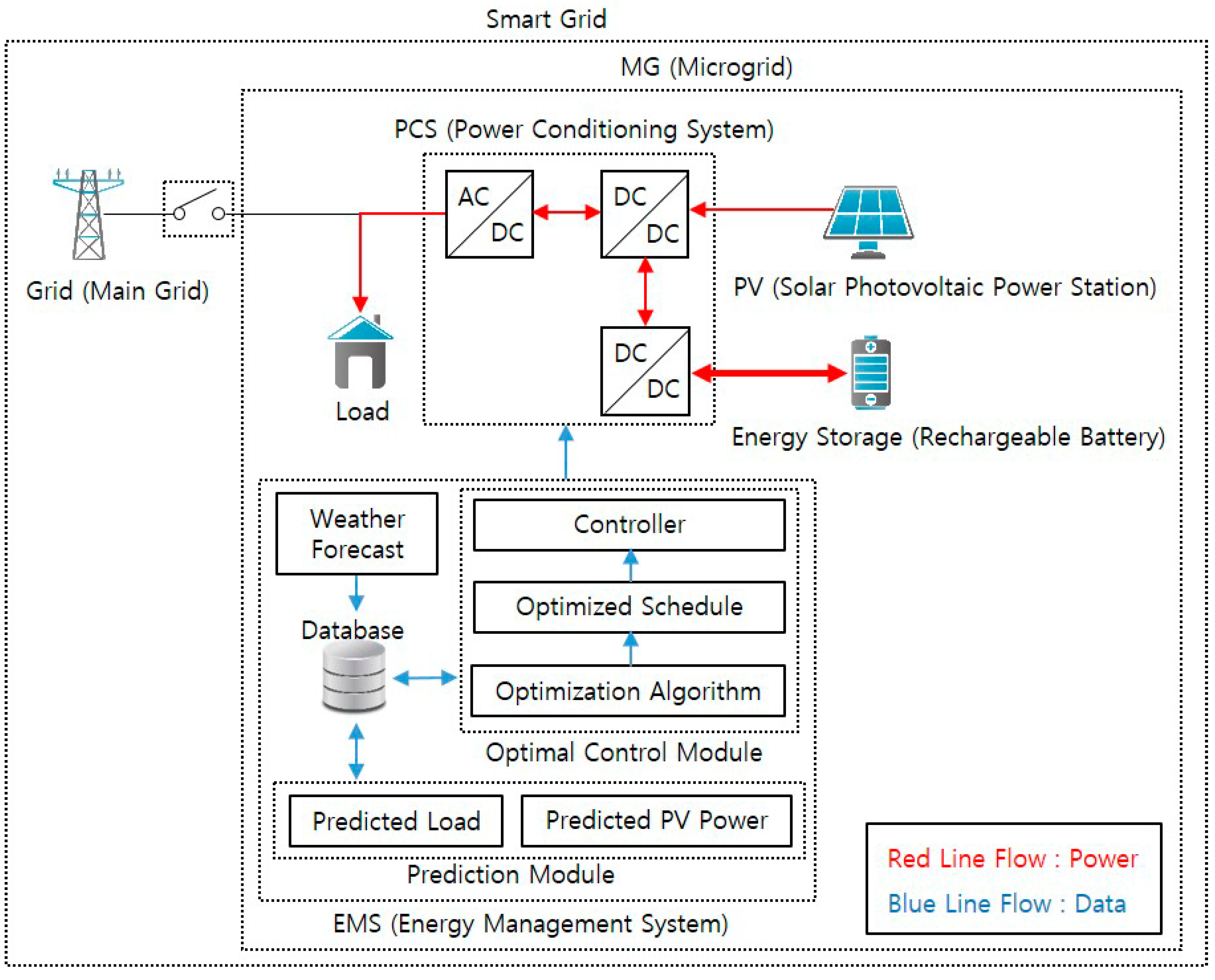
Island mode operates independently from the grid (main grid). The grid (main grid) is the KPX (Korea Power Exchange), the electric company that buys and sells energy (electric energy) in South Korea. In this mode, the supply and consumption of power (electric power) should be done in the microgrid. For example, it can be said that there is a blackout due to the instability of the grid (main grid). An island separated from the grid (main grid) is another example of island mode. In this scenario, as shown in Figure 3, island mode consists of the grid (main grid), load, PCS (power conditioning system), PV (solar photovoltaic power station), energy storage (rechargeable battery), and EMS (energy management system). In Figure 3, the red line is the flow of electric power, and the blue line is the flow of data.

4.1.1. Considerations in PCS (Power Conditioning System)

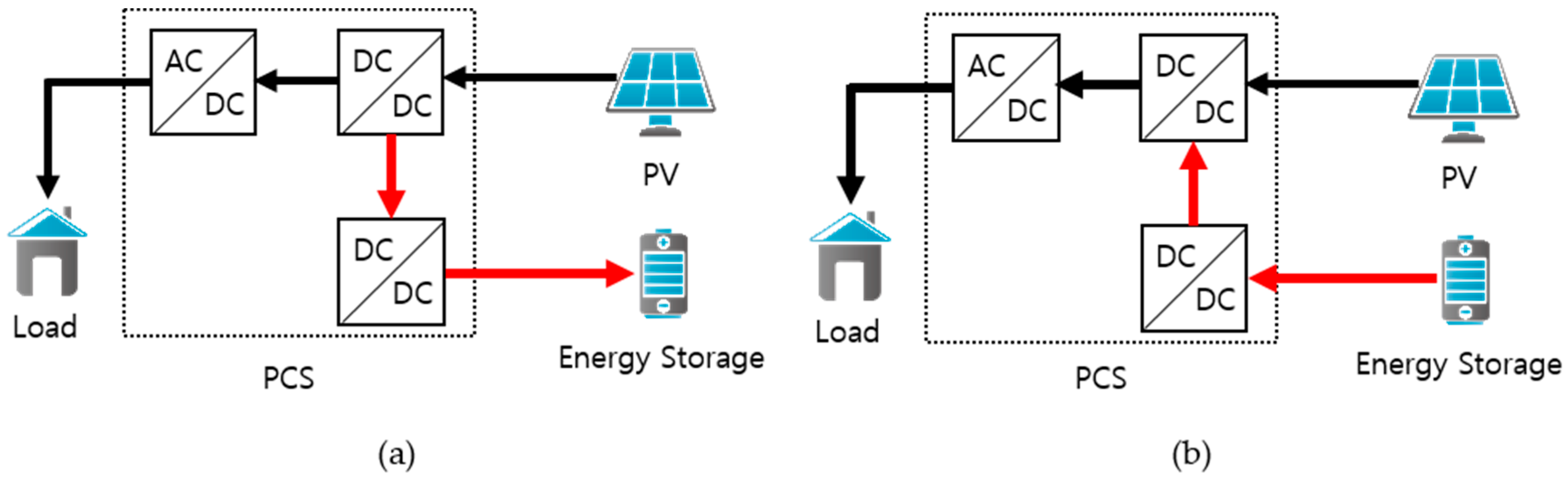
PCS is a semiconductor device that can control power in both directions, converting AC (alternative current) to DC (direct current) or DC to DC. PCS is controlled by EMS, as shown in Figure 4.

Figure 4 shows the energy flow of energy storage with PV production in island mode. Figure 4a shows the energy flow in the charge mode of energy with PV production when the grid is open. Figure 4b shows the energy flow in the discharge mode of ESS when the grid is open. If the grid is closed, the PCS can charge or discharge the energy storage (battery) according to the schedule of the optimization algorithm in EMS.

4.1.2. Considerations in ESS (Energy Storage System)

The ESS is an active energy resource that is controlled by the administrator or operator, unlike the solar photovoltaic power station, which depends on the weather. Active energy resources in a microgrid include wind generation, fuel cells, combined heat and power generation, gas turbine generation, and combined-cycle (both gas turbine and steam turbine) power plants. It is possible to control power generation at any time, if necessary, and incur additional costs, such as fuel, in their electric power production. It is essential for the efficient use of energy in the microgrid, in which considerations, such as a stable power supply and power quality, are necessary. The representative example of ESS includes rechargeable batteries, flywheels, and combined air energy storage, and is capable of controlling (charge and discharge) electric power at a desired time. A rechargeable battery of the ESS has a quick response to the variability for the generation of new energy and renewable energy and changes, and the battery can be charged or discharged by the operator. To operate the ESS efficiently, it is necessary to schedule the charge and discharge over the time of the battery by calculating the energy storage state and considering the aging of available storage capacity according to electrochemical characteristics.

The schedule of the optimization algorithm should automatically take into account the SOC (state of charge) of the battery. When the SOC becomes low, the PCS should be controlled through an optimized schedule in which the battery should stop power supply to the load and charge the energy from a PV power station. When SOC is high, the optimized schedule should stop the automatic charging of energy and allow independent operation. In this study, the simulation of an optimized schedule is performed considering the boundary conditions of SOC. A real energy storage system (chargeable battery) provided by ETRI (Electronics and Telecommunications Research Institute, Korea) has been used in the simulation. The hardware specifications of the ESS are shown in

Table 1. Specifications of energy storage system (ESS) (SOC: state of charge).

Charging Power	Discharging Power	Battery Rated Capacity	Initial SOC	Charging/Discharging Efficiency
Minimum: 0 kW	Minimum: 3 kW	40 kWh	50%	80%
Maximum: 20 kW	Maximum: 20 kW

. The maximum and minimum values of charging/discharging power of 3 kW and 19.5 kW, respectively, are used in the simulation, based on the aging of the charging power. In addition, the boundary condition (working range) of the SOC is set to 5%–95% for the battery life due to over-discharge and explosion prevention due to battery overcharge risks.

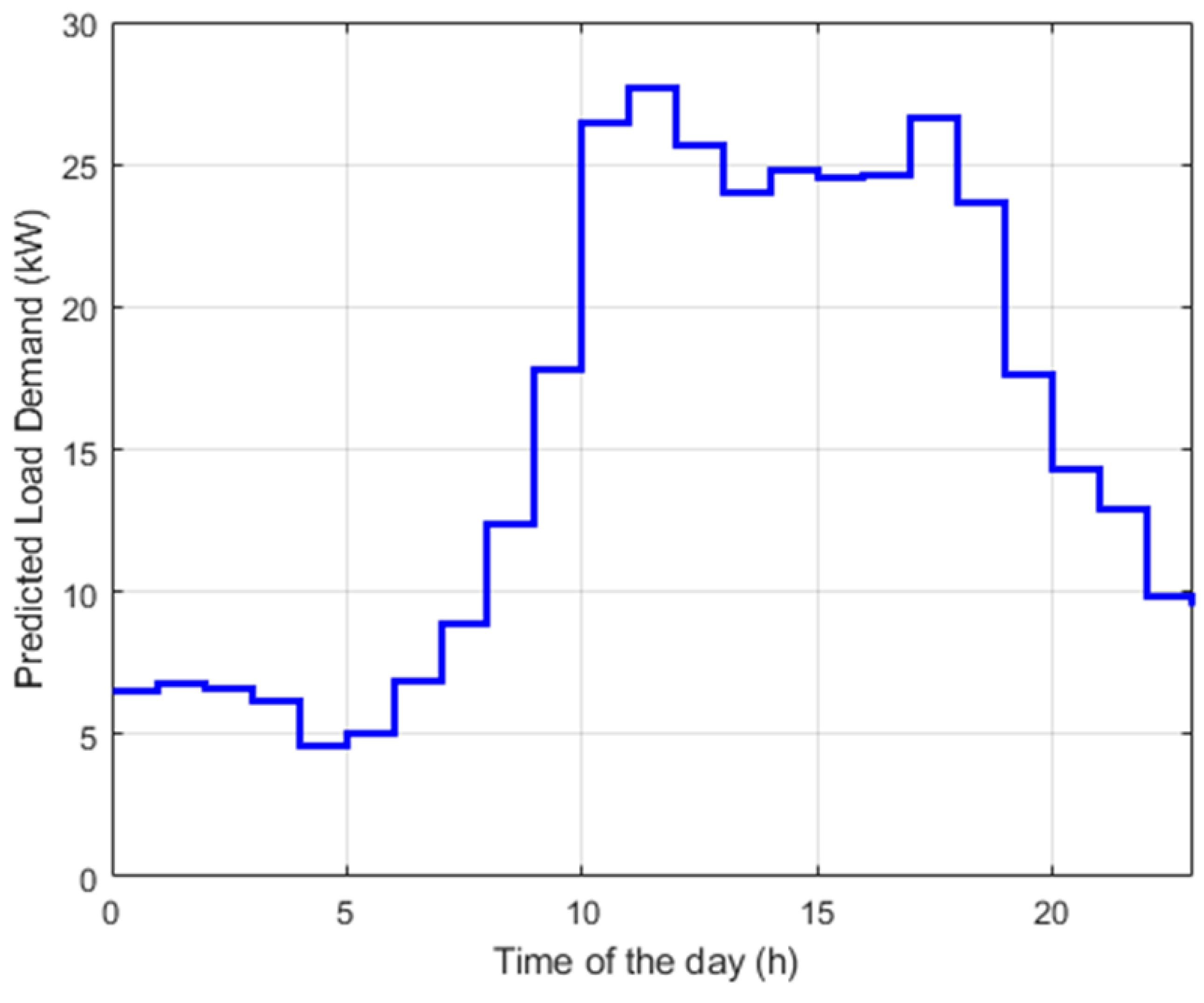
4.1.3. Considerations in Predicted Load Demand

The predicted load demand for business occupancy used in the simulations has been provided by ETRI. The real load has been analyzed for the power consumption environment of twelve buildings in ETRI for three years from 2015 to 2017. Due to the anticipation of the use of EV in the future, consideration has been given to the load in the EV (electric vehicle) charging station infrastructure. The real load used in the simulations has been included in the EV charging station with 3 kW capacity converted from 220 V, 1-Phase AC to 13 A, 60 Hz. The load is a consumption resource that cannot serve as a power supply resource in the microgrid. The model of the predicted load is only considered power consumption in the load. The prediction module in the EMS (energy management system), as shown in Figure 3 receives the weather forecast data and predicts the power consumption of the load. There is uncertainty in the prediction of the power consumption of the load. To solve for the uncertainty, a dip learning algorithm can be applied. In this study, an optimization algorithm was applied to maintain a robust optimization despite the uncertainty of demand (consumer power demand) prediction. The predicted load demand to be used for the optimal control of the ESS is shown in Figure 5.

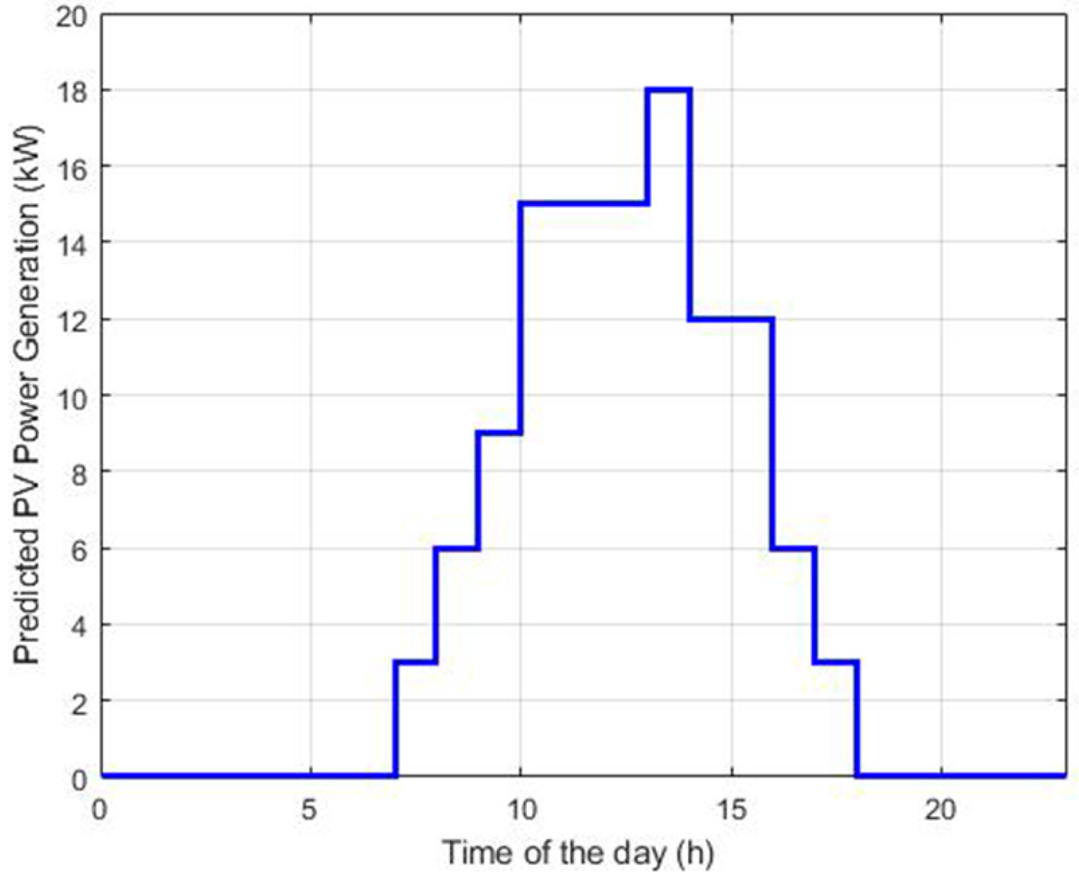
4.1.4. Considerations in Predicted PV Power Generation

The predicted PV power generation in the solar PV power station (up to 30 kW capable) provided by ETRI has been used in the simulation. The PV power station is the passive production resource in the microgrid and is not subject to control, but is necessary to predict the amount of PV power production. Power production can be predicted from weather forecast data through the prediction module in the EMS. There is uncertainty in the weather forecast itself, which is used as an input in predicting the PV power generation. There is also uncertainty in the prediction of PV power generation itself. For the optimal operation of ESS, we derive the control schedule of active resource (ESS) for the future. The predicted load and PV power given as an input is used to derive the optimal control schedule of the ESS, based on the economic operation in the microgrid. In this study, an optimization algorithm was applied to maintain a robust optimization despite the uncertainty in the supply (PV power station) prediction. The predicted PV power generation (kW) to be used for the optimal control of the ESS is shown in Figure 6.

4.2. Effect of Optimization Algorithm using ESS with PV and Grid

An optimal operation scheduling function applied together with external operating conditions is described in this subsection. The following inputs in the external control rules are checked in connection with the peak control against rapidly increasing power consumption: the performance of individual rules when there is a multiple (n) number of peak control rules, time (hour)-based control initiation and completion time, power peak value, and the safety factor following the application of a peak value. If it is necessary to create an optimal operating schedule under another schedule, input values should be changed. The following inputs in the external control rules are checked in connection with the net-zero energy operating control: performance of individual rules when there is a multiple (n) number of peak control rules, time (hour)-based control initiation, and completion time. If it is necessary to create an optimal operating schedule under another schedule, the input values should be changed. The software should be run, and the results obtained should be checked by applying peak control, demand response, and net-zero energy operation conditions.

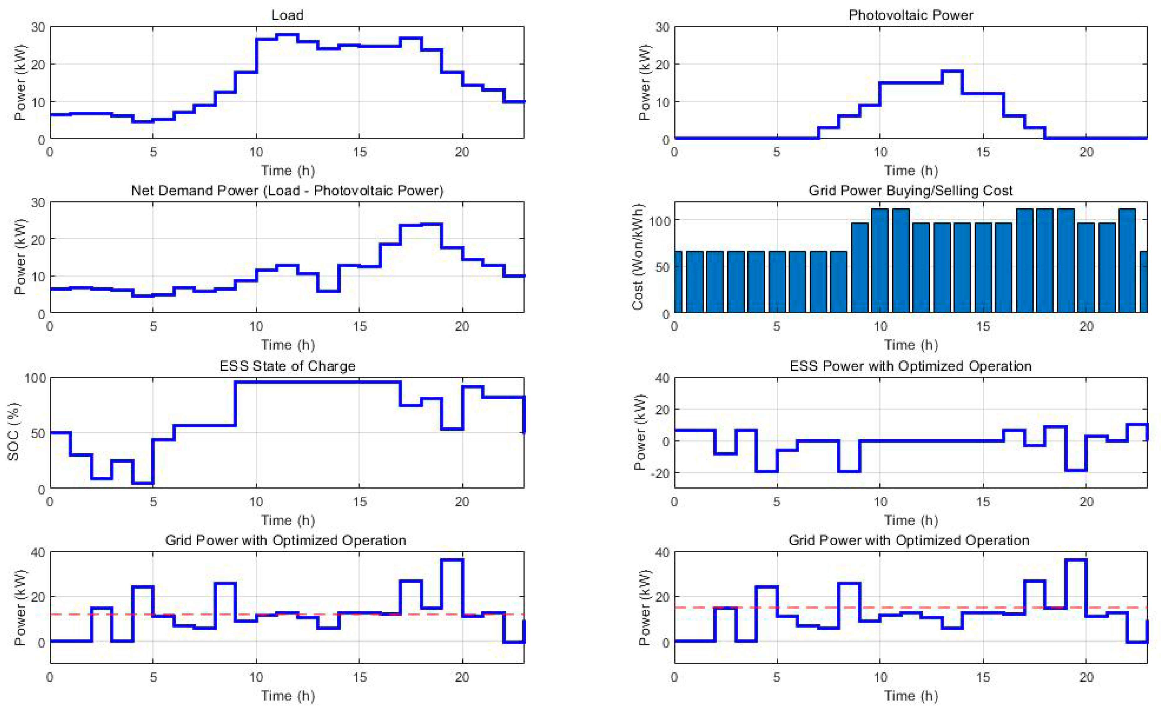
The results of peak control, demand response, and net-zero energy operations have been output to the optimal operating schedule output XML file, and the results are shown in Figure 7. From the data output below, the costs to be paid to the grid when the energy storage was not used and when it was used under the optimal operating schedule were checked to confirm the economic cost. As the cost resulting from using the ESS under the optimal operating schedule was 24,370.8, whereas the cost incurred from not adopting the same schedule was 24,586.3, resulting in a savings of 215.5.

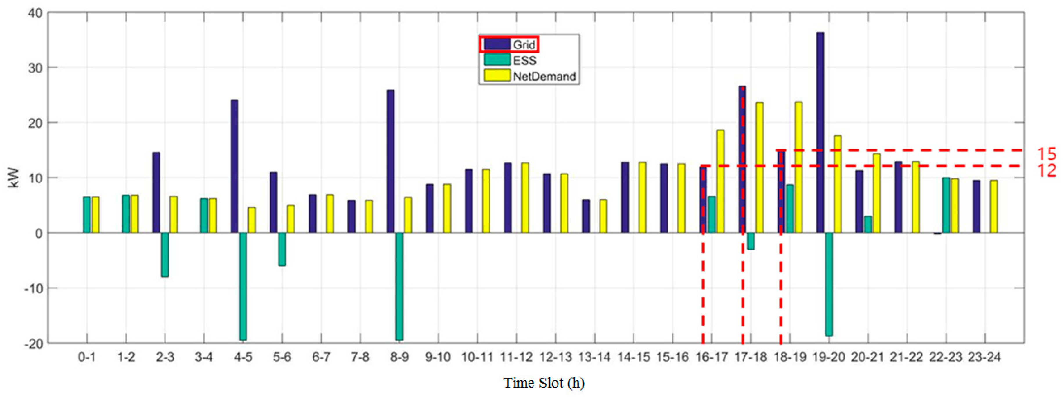
In the case of peak control, 15 × 0.8 = 12 kW was applied to the time of 16–18 h, and 15 kW was applied for 18–19 h. In this case, the conditions were satisfied, but at 17–18 h, the conditions were not satisfied, as the result was 26.6. Figure 8 shows such results.

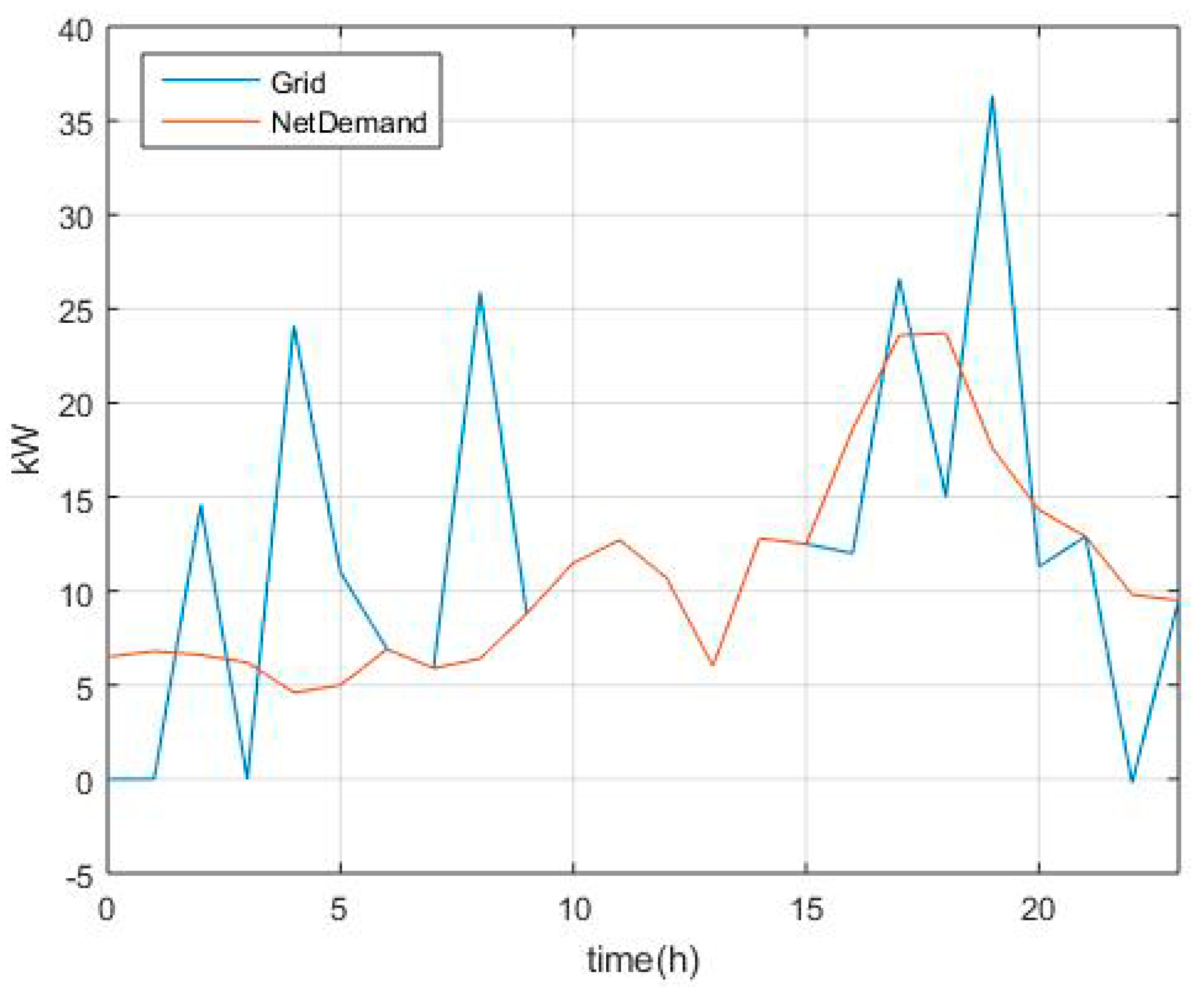
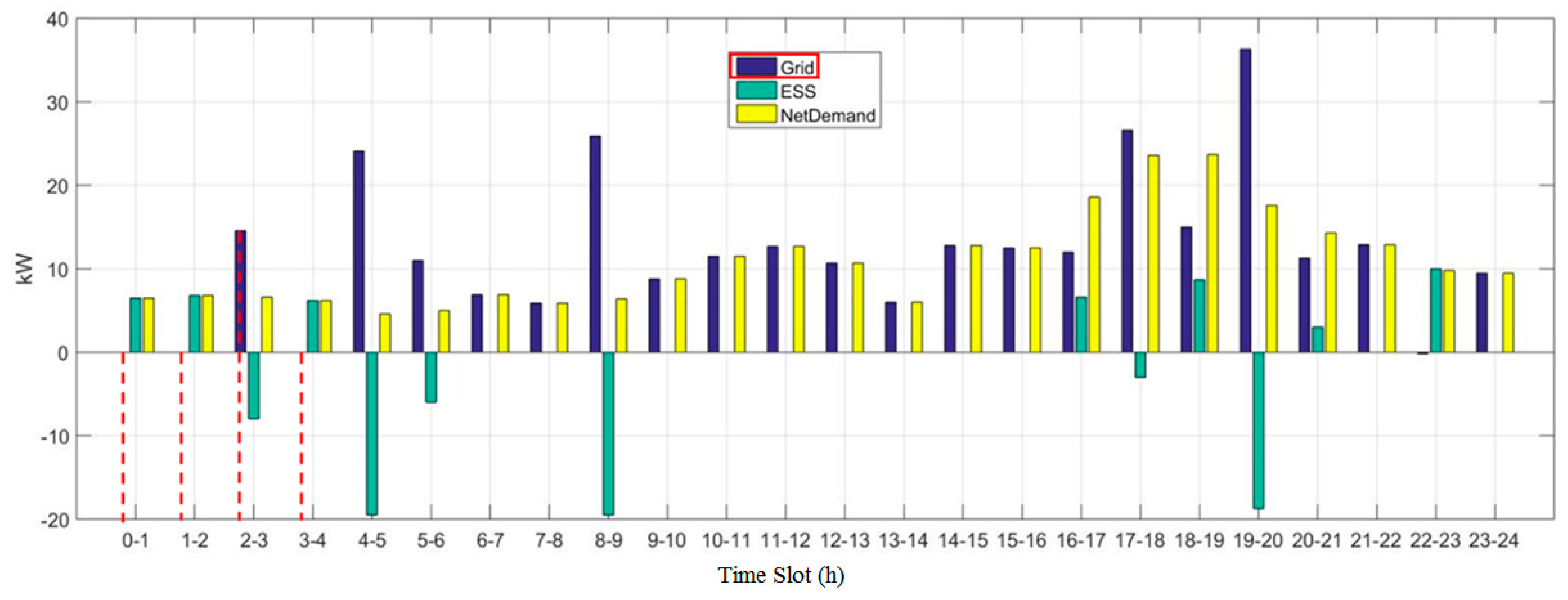
The data below demonstrates that the net demand power at 20–21 h was 14.3 kW whereas the grid power was 11.3 kW, which was a reduction of more than 2 kWh. Meanwhile, at 22–23 h, the values were 9.8 and −0.2, respectively, showing that more than 10 kWh was saved. The results are shown in Figure 8.

Table 2. The peak control operating conditions.

Condition No.	Time Setting (h)	Peak Setting
Condition 1	16–18	12 kW
Condition 2	17–19	15 kW

shows that the starting time in each time slot corresponds to a certain coordinate on the X-axis of the graph. For example, coordinate 16 corresponds to the time of 16–17 h. Second, 12 kW and 15 kW peaks have been set for the time of 16–18 h and 17–19 h, respectively. In such a case, the 12 kW peak (lower peak) is applied to the time slot of 17–18 h so that the installed ESS will initiate its operation to maintain the power usage to be lower than the set value. That is, an optimization schedule minimizing the cost will be in effect. Third, since the power usage of the grid in the time slot of 16–17 h was lower than the 12 kW peak, it satisfied the condition. Next, since the grid’s power usage in the time slot of 17–18 h was 26.6 kW, the condition was not satisfied as it exceeded the 12 kW peak. Finally, as the power usage of the grid was 15 kW in the time slot of 18–19 h, the 15 kW peak limit was satisfied.

The result of applying the net-zero energy operating conditions in the time period of 0–4 h is shown in Figure 8, demonstrating that the conditions were not satisfied in the time slot 2–3 h only, but even so, the next best schedule was derived.

The DR scheme allows the ESS to initiate its operation to save the power used by the grid according to the set condition(s). The condition of net demand − grid = 0 should be met without the ESS, but if the condition net demand − ESS power − grid = 0 can be satisfied by running the ESS, the condition net demand − grid > 0 will be achieved. The power usage saved by running the ESS can be calculated from net demand − grid.

In Figure 9, the starting time in each time slot corresponds to a certain coordinate on the X-axis of the graph. For example, the coordinate 20 corresponds to the time slot of 20–21 h where the net demand was 14.3 kW, and the grid power usage was 11.3 kW. As the difference obtained from net demand was 3 kW, more than 2 kW power was saved in an hour. Accordingly, in the time slot of 22–23 h (net demand = 9.8 kW, grid power usage = −0.2 kW), it is possible to compute that more than 10 kW was saved in an hour. Also,

Table 3. The peak control operating conditions (2).

Condition No.	Time Setting (h)	Peak Setting
Condition 1	21:00–24:00	10 kW
Condition 2	20:00–20:30	2 kW

shows the peak control operating conditions.

An optimal operation scheduling function applied with the internal operating conditions is described in this subsection.

The ESS specification data is checked first, and the minimum and maximum power capacities for both charging and discharging as well as the energy storage capacity and charging efficiency are set. At this time, the basic rules set by the manager should be readjusted if they contradict the specification data.

Next, an expected input error corresponding to the internal operating conditions is set. The power supply schedule received by the optimal operating schedule derivation software as an input value is a predicted value of the future and could be different from the actual value. For example, if the manager entered a predicted value of 20 but he/she expects the power supply schedule will have a value within the range of 16 [= 20 × (1 − 0.2)] to 24 [(=20 × (1 + 0.2)], he/she should set the value as 0.2. Then, the possibility of flattening, which corresponds to the internal operating conditions, is set. Input 1 corresponds to flattening performed regardless of economic loss, while input 0 corresponds to all other conditions. The software is run and checked to determine whether a time-based power schedule has been derived conforming to the ESS specification data. The differences in the mean values, minimum values, and maximum values of the expected time-based grid power use schedule are checked, following the changes in the predicted input error. Finally, whether the flattening of the schedule has been performed according to the settings is checked.

The specification data of ESS was checked and amended as needed. The amended items are as follows: power capacity unit, storage capacity unit, minimum power capacity of charging, maximum power capacity of charging, minimum power capacity of discharging, maximum power capacity of discharging, energy storage capacity, charging efficiency, and discharging efficiency. Additionally, the basic rules have been readjusted when they contradict the specification data. The items which have been amended when checking the internal operating rules are the expected input error proportion and the possibility of flattening. After checking ESS power to grasp whether the schedule had been derived according to ESS specifications, confirmation was made, as the results underlined below did not deviate from the individual setting ranges. Also, the tests to check whether the charging power capacity (0–20 kW), discharging power capacity (3–20 kW), charging (3–19.5 kW)/discharging (3–19.5 kW) capacity set by the manager, and the mean/minimum/maximum value of the expected time-based grid power use schedule (Grid) had been derived correctly according to the expected input error.

Since only the time slot of 2–3 was Grid > 0 among the other time slots (0–1, 1–2, 2–3, and 3–4), the condition of net-zero energy was not satisfied, but it was possible to establish that the next best schedule had been derived in the same time slot.

Meanwhile, the data reflected in the optimal operating schedule function when the internal operating conditions are applied may have some margin of error in expected values when sunlight generation and loads are taken into consideration. The supply-demand equation can be reformulated as (Load + dL) − (PV + dP) − ESSP − Grid = 0(Expected), which can be finalized as Load − PV − ESSP − (Grid + dG) = 0, by combining dL (error in load), dP (error in sunlight generation), and dG (error in grid). In other words, by considering the error in the grid, an effect similar to the one obtainable from the equation, considering the errors in PV and load, can be obtained. Figure 10 shows the result of the expected input error.

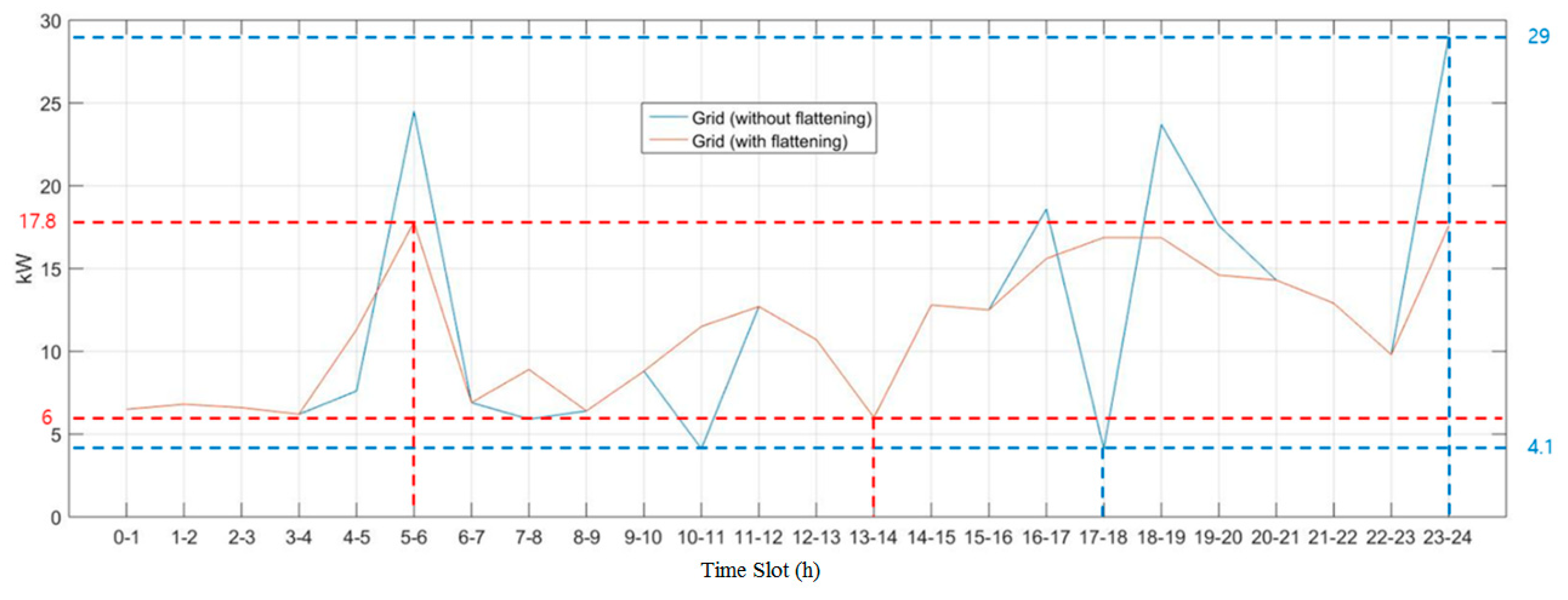
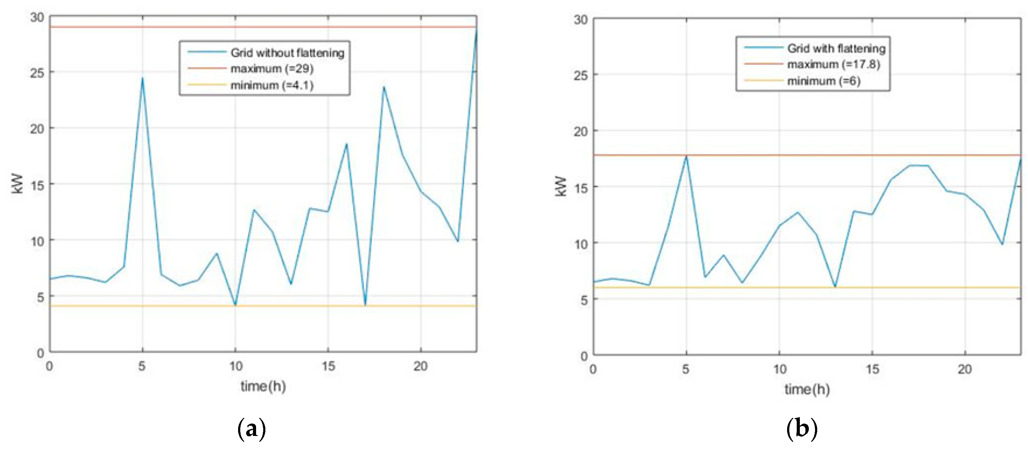
The large difference in the grid’s maximum and minimum values would cause a rapid change so that it is not desirable. In that case, flattening is applied to reduce rapid change in the grid power. After applying the grid-flattening condition, as shown in Figure 11, grid power usage to which flattening was unapplied (applied) is shown in the left (right). It is possible to recognize that the difference between the maximum and minimum values has been reduced from 24.9 (=29 − 4.1) to 11.8 (=17.8 − 6).

5. The Microgrid Test for the Stability of Operations Performed by the Small- and Medium-sized Enterprises in Industry 4.0

The manager sets the control period (Time.T), corresponding to the configurable basic control rules. The control period is entered by the hour for the period in which the optimal operating schedule will be derived, and the basic value is 24 (1 day). Similarly, the manager sets the unit time (Time.dt), corresponding to the configurable basic control rules so that the optimal operating schedule will be derived for every unit time, and the basic unit time is 1. The unit time can be set by minutes, which should be converted into units of hour. For instance, 30 min should be represented as 0.5 h for input. If the control period is 24 and the unit time is 1, the 24 schedules (i.e., from 0–1 h to 23–24 h) will be output.

Next, the manager sets the maximum and minimum charge amount values (ESS.P_ESS_chg_min/max) for the ESS, along with the maximum and minimum discharge amount values for the same ESS in units of hour, following the configurable rules. Then, the software is run, and the ESS operating schedules (ESS.Power) are checked.

5.1. Process for Stability and Results

For the experiment, the values of the control period and the unit time were set at 24 and 1, respectively, whereas a rule that regulates the ESS to be charged as much as 5 kW in the time slot 2–3 was entered. After running the software, it was confirmed that the schedule shown in

Table 4. The Hour-based ESS Operating Schedules.

Time Slot	0–1	1–2	2–3	3–4	4–5	5–6	6–7	7–8	8–9	9–10	10–11	11–12
ESS.Power	−17.5	0	−5	0	0	0	0	0	0	0	17.08	0
Time Slot	12–13	13–14	14–15	15–16	16–17	17–18	18–19	19–20	20–21	21–22	22–23	23–0
ESS.Power	0	0	0	0	0	0	0	0	0	0	9.8	19.5

was output.

From Table 4, it is possible to confirm that the amount of 5 kW was charged in the time slot 2–3, following the schedule under the specified rule.

5.2. Testing Method for Stability

The time-slot-based predicted input is checked for the power demand schedule, and the value(s) are changed if a derived optimal operating schedule is needed under a different schedule. The same procedure is repeated for the power supply schedule and the unit cost of production. The software is run and the cost required to settle with the grid is checked (TotalCost.WithoutESS.Normal), which can be obtained by calculating (total demand of time slot i) × (unit cost of time slot i) first for each time slot and then aggregating all of the resulting values for the case when ESS was not used. However, if the ESS was used under the optimal operating schedule, the cost to be settled with the ESS (TotalCost.WithESS.Normal is determined by calculating (system power usage of time slot i) × (unit cost of time slot i) × (unit time) for each time slot and adding up the resulting values.

5.3. Stability Test Process and Results

In

Table 5. The predicted values of power demand.

Time Slot	0–1	1–2	2–3	3–4	4–5	5–6	6–7	7–8	8–9	9–10	10–11	11–12
Load	6.5	6.8	6.6	6.2	4.6	5	6.9	8.9	12.4	17.8	26.5	27.7
Time Slot	12–13	13–14	14–15	15–16	16–17	17–18	18–19	19–20	20–21	21–22	22–23	23–0
Load	25.7	24	24.8	24.5	24.6	26.6	23.7	17.6	14.3	12.9	9.8	9.5

,

Table 6. The predicted values of power supply schedule.

Time Slot	0–1	1–2	2–3	3–4	4–5	5–6	6–7	7–8	8–9	9–10	10–11	11–12
PV	0	0	0	0	0	0	0	3	6	9	15	15
Time Slot	12–13	13–14	14–15	15–16	16–17	17–18	18–19	19–20	20–21	21–22	22–23	23–0
PV	15	18	12	12	6	3	0	0	0	0	0	0

and

Table 7. The expected power supply unit cost schedule.

Time Slot	0–1	1–2	2–3	3–4	4–5	5–6	6–7	7–8	8–9	9–10	10–11	11–12
UnitBuy	66.1	66.1	66.1	66.1	66.1	66.1	66.1	66.1	66.1	96.5	111.3	111.3
UnitSell	66.1	66.1	66.1	66.1	66.1	66.1	66.1	66.1	66.1	96.5	111.3	111.3
Time Slot	12–13	13–14	14–15	15–16	16–17	17–18	18–19	19–20	20–21	21–22	22–23	23–0
UnitBuy	96.5	96.5	96.5	96.5	96.5	111.3	111.3	111.3	96.5	96.5	111.3	66.1
UnitSell	96.5	96.5	96.5	96.5	96.5	111.3	111.3	111.3	96.5	96.5	111.3	66.1

, the predicted values of the power demand schedule, power supply schedule, and unit cost schedule for all of the time slots have been entered, respectively.

After the software was run and the cost to be settled with the grid when the ESS was not used (TotalCost.WithoutESS.Normal), the same cost when the ESS was used under the optimal operating schedule were checked to calculate the profit (cost saved). As the costs of the former and the latter were 24,586.3 and 24,370.8, respectively, the financial gain (cost saved) was 215.5 when the ESS operated under the optimal operating schedule.

5.4. A Function Deriving an Optimal Operating Schedule under External Operating Conditions

5.4.1. Test Method

To maintain control under external operating conditions, the following method is performed. To specify how to perform peak control in the event of a rapid increase in demand, check whether (PC.Grid_buy.Flag) the individual rule (idx = “i”, 1 ≤ i ≤ n) has been followed for each peak control rule (PC.Grid_Buy, size = “1 × n”), and if at the starting and ending times (PC.Grid_Buy.TimeStart, PC.Grid_Buy.TimeEnd), the peak values (PC.Grid_Buy.PeakPower) are entered in kW, and the safety factors following the application of peak time values (PC.Grid_Buy.SafetyFactor) are entered. To derive another optimal operating schedule under different conditions, change these inputs.

For the external control rule concerning the demand response (DR) signals, check whether (DR.Flag) the individual rule (idx = “i”, 1 ≤ i ≤ n) has been followed for each DR control rule (DR, size = “1 × n”), and if at the starting and ending times (DR.TimeStart, DR.TimeEnd), the energy-saving goal (DR.DRSavingTotal) is entered in kWh, and the safety factors following the application of the energy-saving goals (DR.SafetyFactor) are entered. To derive another optimal operating schedule under different conditions, change these inputs.

5.4.2. Test Process and Results

The external operating rules have been modified as the rules in

Table 8. Peak control operating condition.

	idx	Application (Flag)	Time Slot	Peak Setting
Condition 1	1	Applied (Flag = 1)	16–17, 17–18 h	15 × 0.8 kW
Condition 2	2	Ignored (Flag = 0)	16–17, 17–18, 18–19 h	10 × 1.0 kW
Condition 3	3	Applied (Flag = 1)	17–18, 18–19 h	15 × 1.0 kW

,

Table 9. DR (Demand Response) operating condition.

	idx	Application (Flag)	Time Slot	DR Setting
Condition 1	1	Applied (Flag = 1)	21–22, 22–23, 23–24 h	10 × 1.0 kWh
Condition 2	2	Ignored (Flag = 0)	21–22, 22–23, 23–24 h	30 × 1.0 kWh
Condition 3	3	Applied (Flag = 1)	20–20.5 h	2 × 1.0 kWh

and

Table 10. Net-zero operating condition.

	idx	Application (Flag)	Time Slot
Condition 1	1	Applied (Flag = 1)	0–1, 1–2, 2–3
Condition 2	2	Ignored (Flag = 0)	3–4, 4–5
Condition 3	3	Applied (Flag = 1)	1–2, 2–3, 3–4

.

After the software is run, it is checked whether the application results of peak control (ExtCond.PC.GridBuy), demand response (ExtCond.DR), and net-zero operation (ExtCond.IO.Grid) have been output in the optimal operating schedule XML file (zmoc.optim.result.cfg.xml). The results are shown in Figure 12, Figure 13 and Figure 14.

For peak control, 12 kW (15 × 0.8) and 15 kW were applied to the time slots 16–17 & 17–18 and 17–18 & 18–19, respectively. That is, the system power usages were limited to 12 kW and 15 kW for the time slots 16–17 & 17–18 and 17–18 & 18–19, respectively. However, for the time slot 17–18, in which the conditions overlap, the smaller power usage limitation (12 kW) was applied. The time slots 16–17 and 18–19 contained grid power usages of 12 kW and 15 kW each, satisfying Conditions 1 and 3 of Table 5. On the other hand, the time slot 17–18 (26.6 kW) failed to satisfy Condition 1. The application results of the peak control are shown in Figure 12.

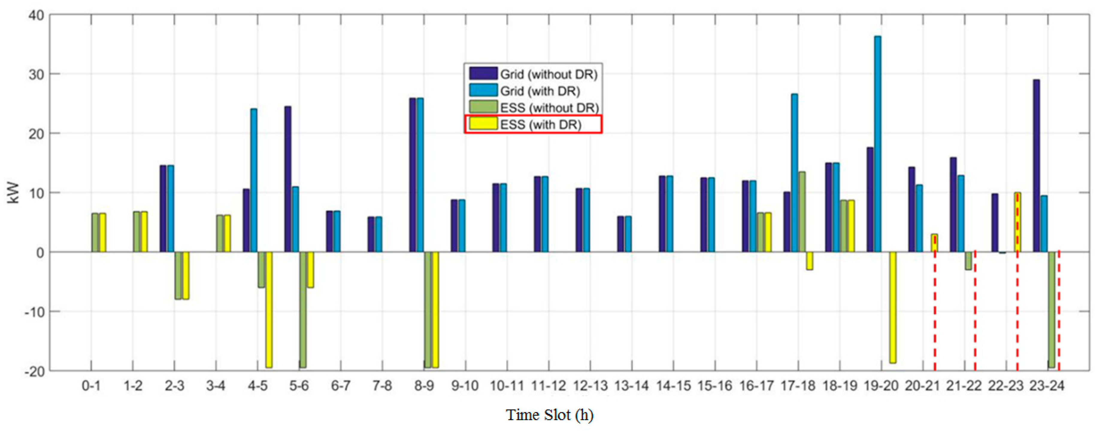
The application results of demand response are shown in Figure 13. When the demand response was set, as much as 10 kW and 3 kW were discharged from the ESS for the time slots 22–23 and 20–21, respectively. Since the ESS supplied a 10 kWh (=10 kW × 1 h) amount of power for the time slot 22–23, it was clear that Condition 1 of Table 6 (i.e., supplying 10 kW power to the ESS) had been satisfied. Also, for a power of 1.5 kW (3 kW × 0.5 h) supplied by the ESS, Condition 3 of Table 9 (supplying 2 kW to the ESS for the time slot 20–20.5) was not satisfied.

The application results of the net-zero energy operating condition, giving the system power usage from hour 0 to hour 4 shown in Figure 14, which shows that the condition was not met as the system power usage was not 0 for the time slot 2–3. However, it is possible to know that the second-best schedule has been derived, even though the external operating condition has not been satisfied.

5.4.3. A Function Deriving an Optimal Operating Schedule under Internal Operating Conditions

Optimal Operating Schedule Test Method

To maintain control under internal operating conditions, the following method is performed. Check the specification of the ESS first and set the values of minimum charge power capacity (kW) (ESS.P_ESS.chg_min_spec), maximum charge power capacity (kW) (ESS.P_ESS.chg_max_spec), minimum discharge power capacity (kW) (ESS.P_ESS.dis_min_spec), maximum discharge power capacity (kW) (ESS.P_ESS.dis_max_spec), energy storage capacity (kWh) (ESS.ECap_spec), charge efficiency (ESS.Eff_chg), and discharge efficiency. In this case, change the basic rules if earlier basic rules (ESS.P_ESS_dis_min, ESS.P_ESS_dis_max, ESS.P_ESS_chg_min, ESS.P_ESS_chg_max) set by the manager violate the specification.

Set the predicted input error (Net_demand.Err_prop) corresponding to the internal operating conditions. The power supply/demand schedule (Power.PV) received by the optimal operating schedule derivation software as an input is the future predicted value, so that there is a difference between the actual value and the predicted value, such that the maximum value that the absolute value of such a difference can have can be calculated by multiplying the predicted value with the predicted input error. For example, if the predicted value was set to 20 at the beginning, but it was expected to have a value between 16 [20 × (1 − 0.2)] and 24 [(20 × (1 + 0.2)] in the future, set the error at 0.2. Next, set the feasibility of flattening (Grid.Flat.Flag). If the flattening corresponding to the internal conditions is to be performed for the grid usage regardless of economic loss, substitute 1, otherwise set to 0.

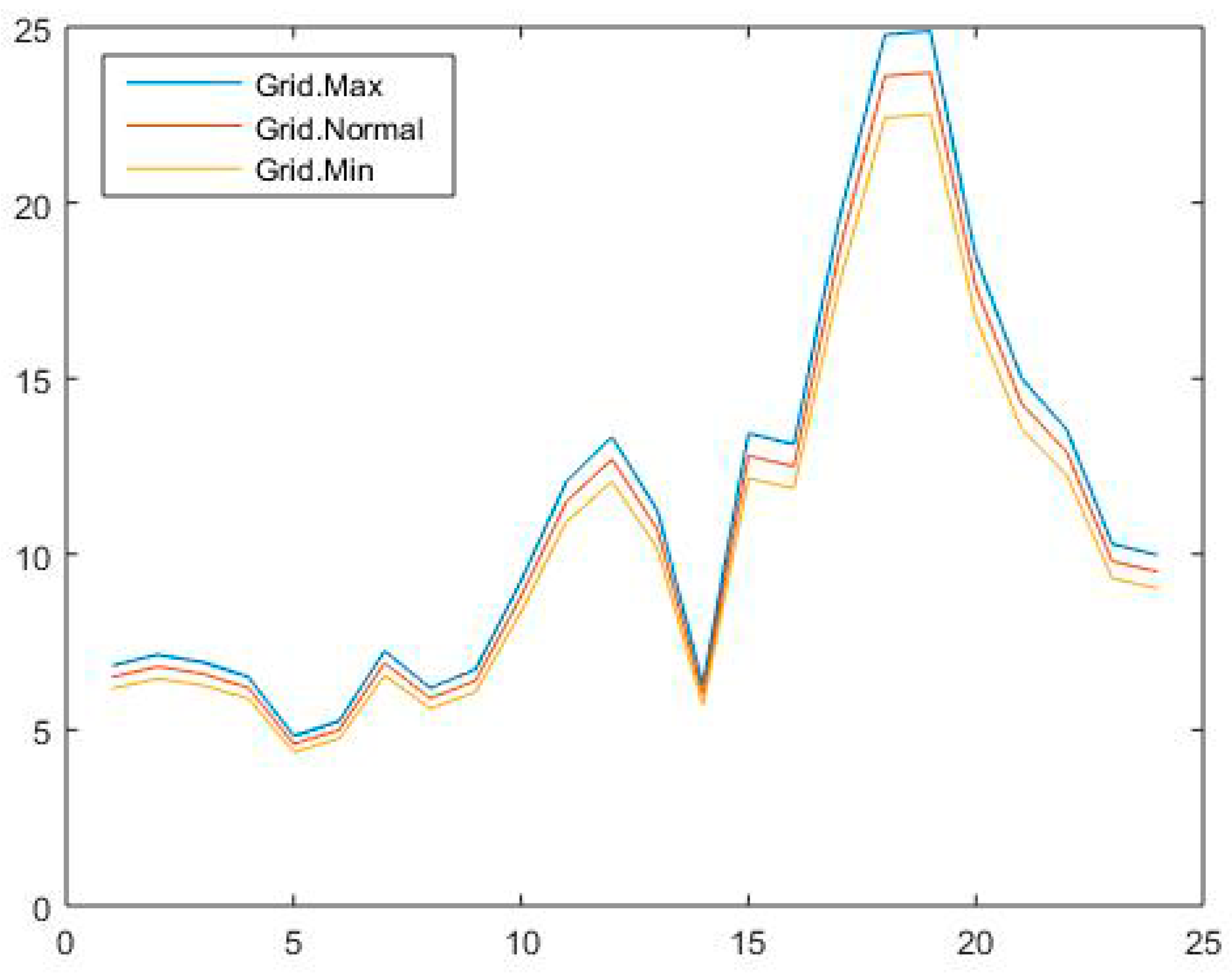
Run the software and check whether each power (kW) schedule (ESS.Power) has been derived in accordance with the ESS specification and confirm that the average value (Grid.Normal), minimum value (Grid.Min), and maximum value (Grid.Max) of each time slot’s predicted grid power usage (kW) have been output correctly based on the predicted input error. Also, confirm that each time slot’s power schedule (ESS.Power) has been flattened following the preset flattening condition (i.e., apply flattening or not).

Optimal Operating Schedule Test Process and Results

The specification of ESS was checked first and modified as needed (Power Capacity Unit: kW, Power Storage Capacity:kWh). Modifications were made to the following: minimum charge power capacity (kW) (ESS.P_ESS.chg_min_spec), maximum charge power capacity (kW) (ESS.P_ESS.chg_max_spec), minimum discharge power capacity (kW) (ESS.P_ESS.dis_min_spec), maximum discharge power capacity (kW) (ESS.P_ESS.dis_max_spec), energy storage capacity (kWh) (ESS.ECap_spec), charge efficiency (ESS.Eff_chg), and discharge efficiency.

Also, adjustments were made for the basic rules set by the manager (i.e., ESS.P_ESS_chg_min, ESS.P_ESS_chg_max, ESS.P_ESS_dis_min, ESS.P_ESS_dis_max, ESS.ECap) when they violated the specification.

Table 11. The basic rules set by the manager.

Min. Charge Power Cap.	Max. Charge Power Cap.	Min. Discharge Power Cap.	Max. Discharge Power Cap.	Energy Storage Cap.	Charge Efficiency	Discharge Efficiency
0 kW	20 kW	3 kW	20 kW	40 kWh	80%	80%

shows the basic rules set by the manager.

The necessary modifications made when checking the internal operating rules were the predicted input error proportion (NetDemand.Err_prop: 0.00 -> 0.05) and the possibility of flattening (Grid.Flat.Flag: 0 -> 1).

Checking whether the optimal operating schedule was derived in accordance with the specification of the ESS after running the software, it was confirmed that the output schedule was fit to the specification as the following conditions (Range of charge power capacity 0–20 kW, Range of discharge power capacity: 3–20 kW) were satisfied.

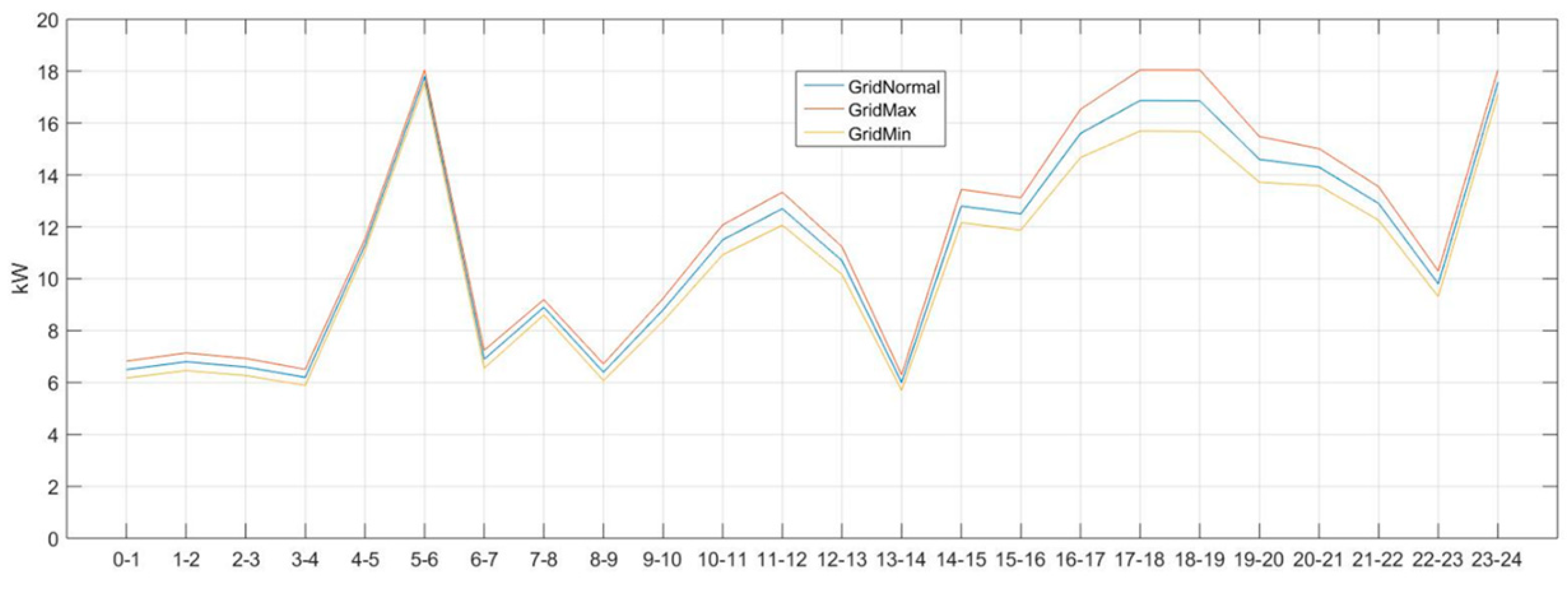
Next, it was checked whether the reference value (Grid.Normal), minimum value (Grid.Min), maximum value (Grid.Max) of manager-set charge range (3–19.5 kW), discharge range (3–19.5 kW), and each time slot’s predicted grid power (kW) use schedule (Grid) had been derived in accordance with the predicted input error (NetDemand.Err_prop). From Figure 15, it was possible to realize that differences occurred depending on the predicted input error proportions, as there were differences in GridNormal, GridMax, and GridMin.

Meanwhile, Figure 16 shows the result after the flattening task, which reduced the difference between the grid’s maximum and minimum values, was applied. The curved red (blue) line is showing the system power usage when the flattening has (not) been applied. The maximum and minimum values of the system power usage is 29 kW and 4.1 kW, respectively, showing a difference of 24.9 kW. On the other hand, when the flattening was applied, the same values were 17.8 kW and 6 kW, respectively, showing a difference of 11.8 kW. This means that the flattening had reduced the difference from 24.9 kW to 11.8 kW.

6. Conclusions

It is essential for consumers of the Industry 4.0 era to utilize an ESS with an optimal design and efficiency, based on predicted future demand by creating an appropriate database aimed at consistently supplying new and renewable energies of good quality. This study focused on the software-based method of deriving an optimal operating schedule for the ESS used in a microgrid, and the method introduced is able to reduce power-related costs by allowing the ESS to perform more efficiently and economically. The software developed solely for this purpose adopts mixed integer linear programming or a genetic algorithm, and is implemented with MATLAB, featuring four major functions with which an optimal operating schedule for the ESS can be derived: when basic operating rules are applied, external operating conditions are applied, internal operating conditions are applied, or another grid is involved in operation.

Optimal operating schedule derivation software is introduced in this study, focusing on data input/output and optimal operating schedule derivation functions. The software was able to derive an optimal ESS operating schedule that maximizes the economics of a microgrid by collecting the basic operating rules, expected supply and demand data of power consumption/production resources, power supply unit cost information, external special events/action information, and internal control setting. The main feature of the software proposed in this study is that the next four functions have been implemented with MATLAB and Python: an optimal operation schedule derivation function when the basic operation rules are applied, when operating with another grid, when the external operating conditions are applied, and finally, when internal operating conditions are applied. It was confirmed through tests that the functions of the operating schedule worked well to find the best schedule or next best schedule (when the given conditions were not satisfied). This study contributes to establishing an optimal microgrid operation schedule in terms of economics by reducing the costs of energy use while maximizing the efficiency of its use on the consumer side, helping to solve our present energy problems. It is expected that future study will focus on more detailed conditions for storage, in addition to introducing a certain type of distributed power source.