A Review of Convex Approaches for Control, Observation and Safety of Linear Parameter Varying and Takagi-Sugeno Systems


Abstract
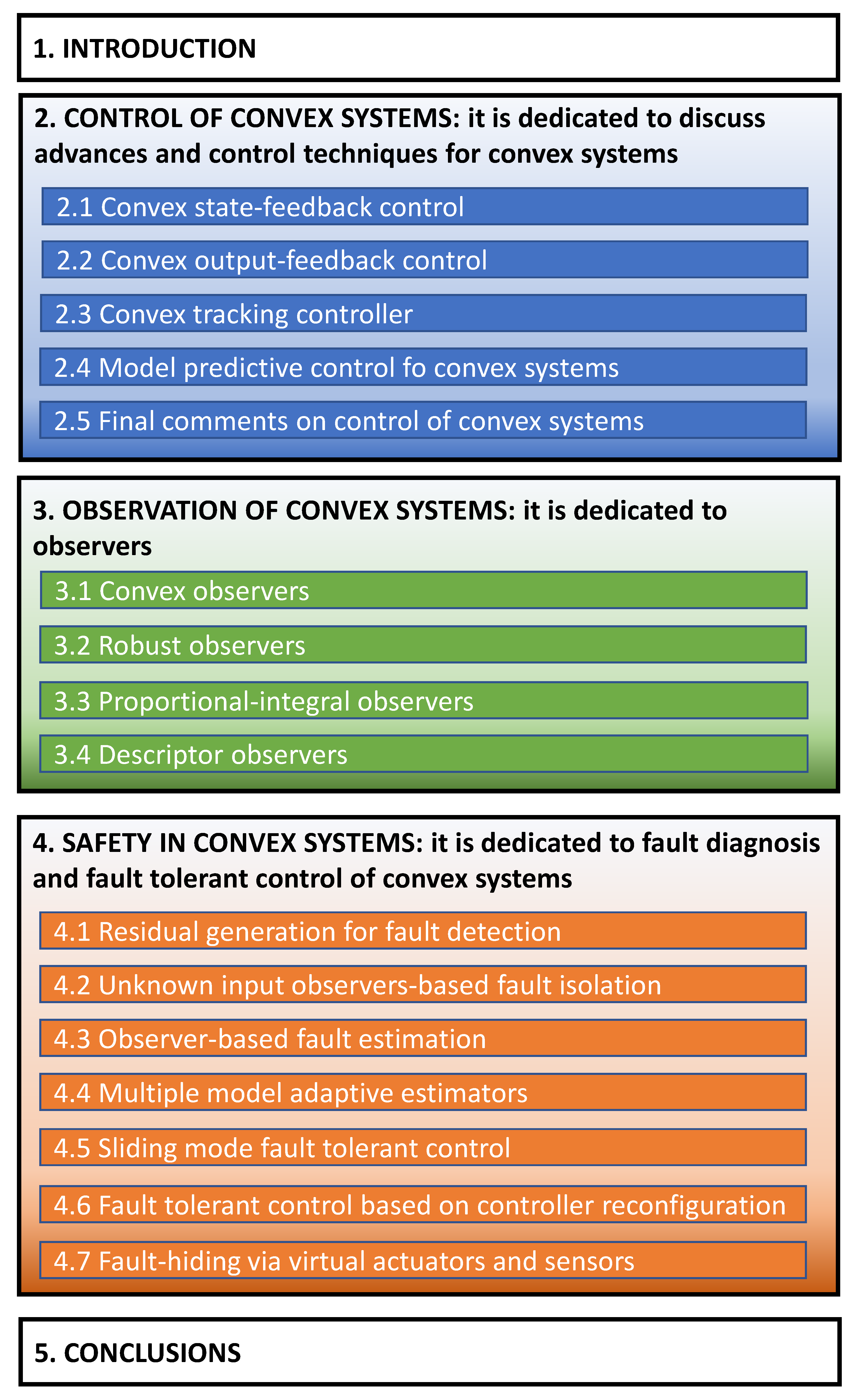
:1. Introduction
2. Control of Convex Systems
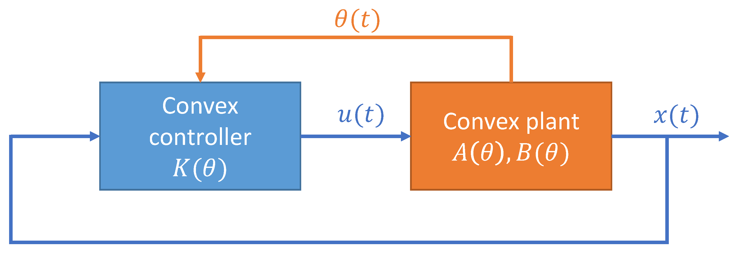
2.1. Convex State-Feedback Control
2.2. Convex Output-Feedback Control
2.3. Convex Tracking Controller
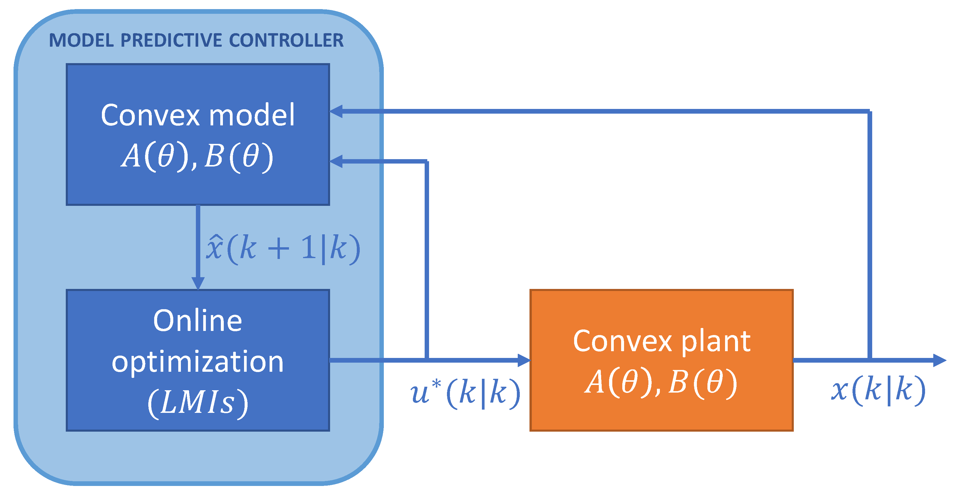
2.4. Model Predictive Control for Convex Systems
2.5. Final Comments on Control of Convex Systems
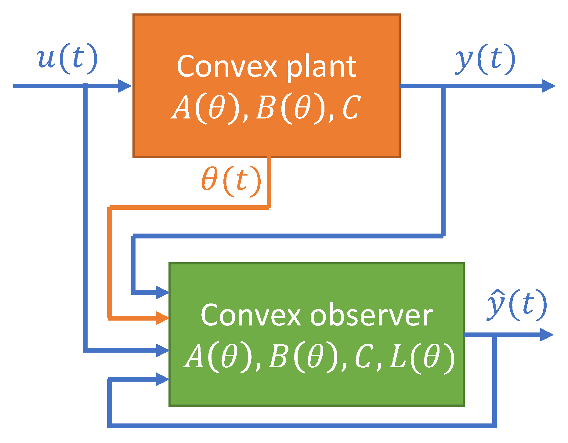
3. Observation of Convex Systems
3.1. Convex Observers
3.2. Robust Observers
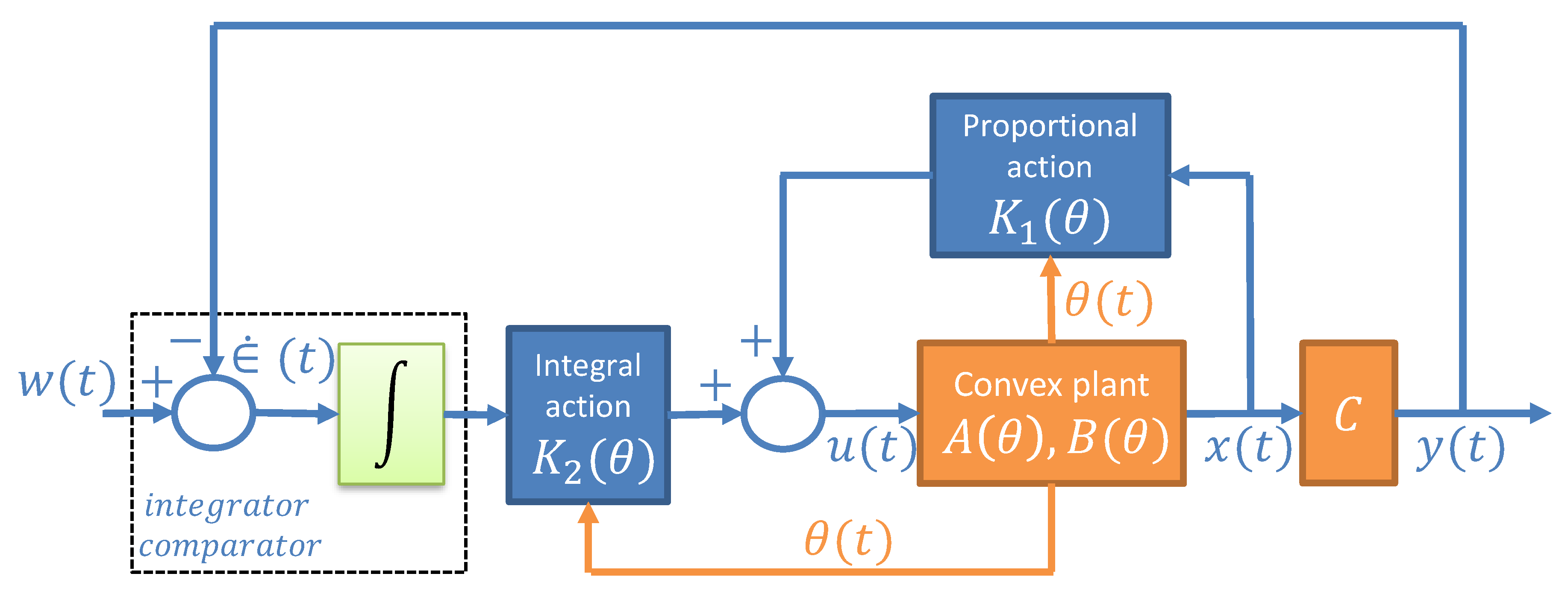
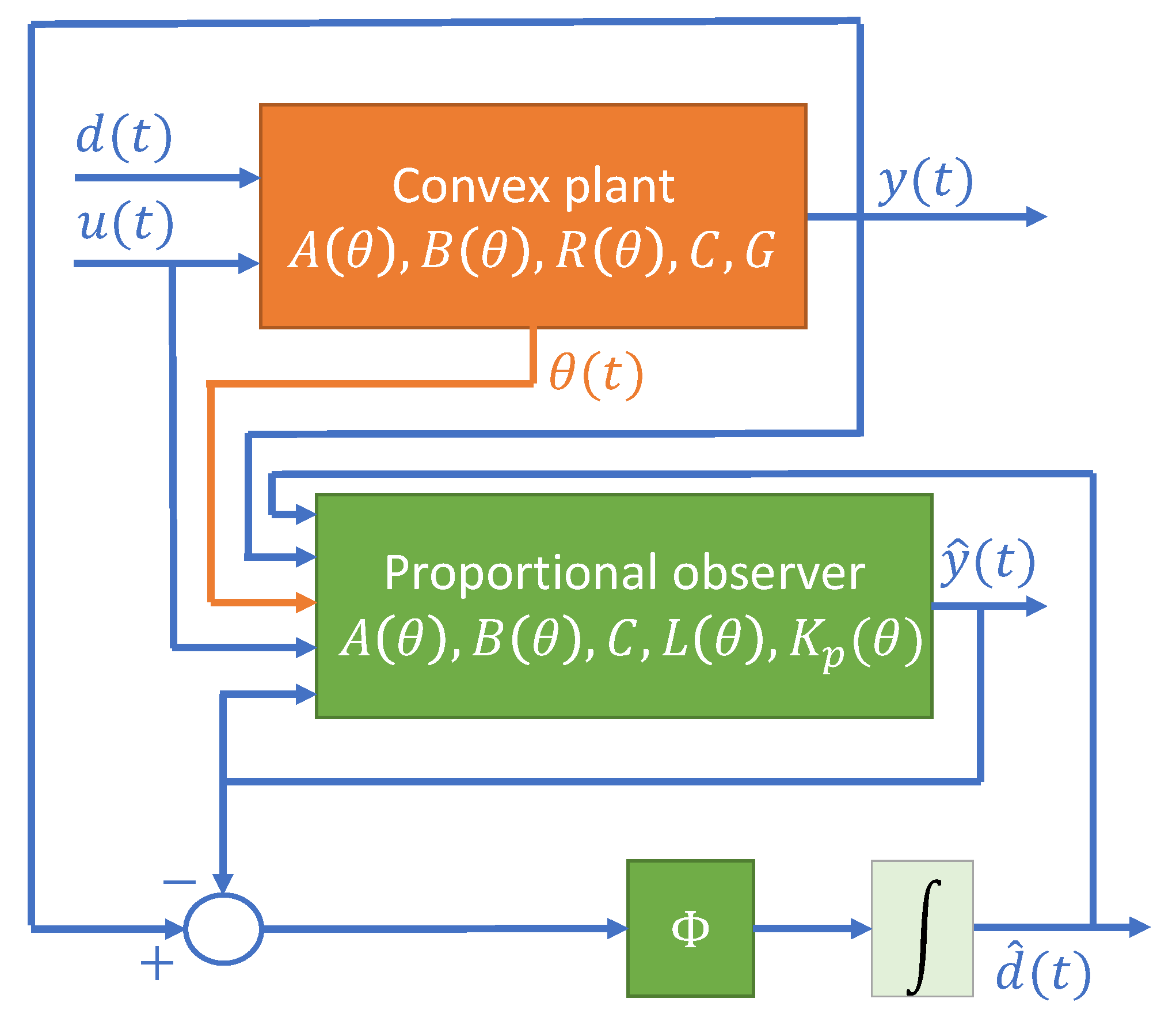
3.3. Proportional-Integral Observers
3.4. Descriptor Observers
4. Safety in Convex Systems
4.1. Residual Generation for Fault Detection
4.2. Unknown Input Observers-Based Fault Isolation
4.3. Observer-Based Fault Estimation
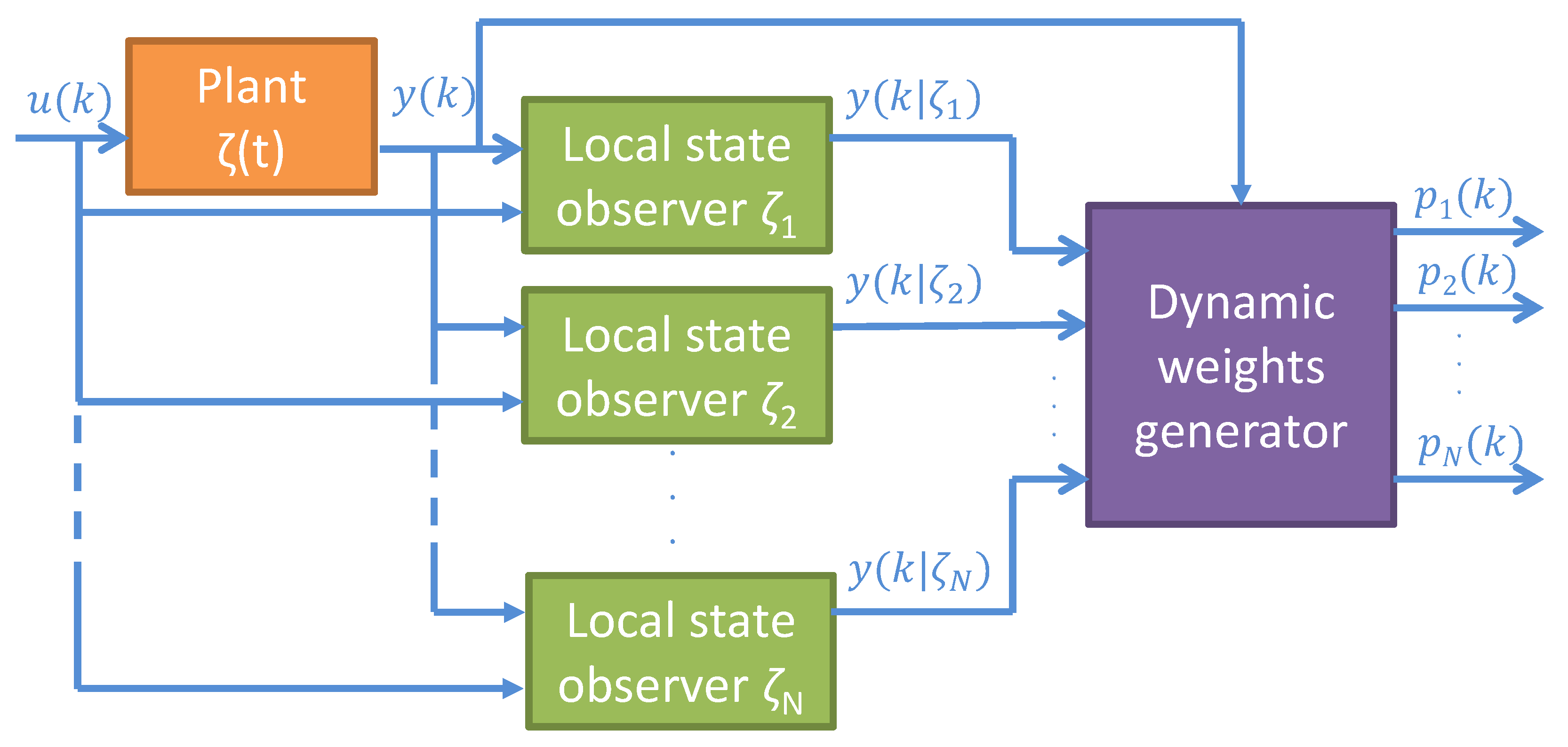
4.4. Multiple Model Adaptive Estimators
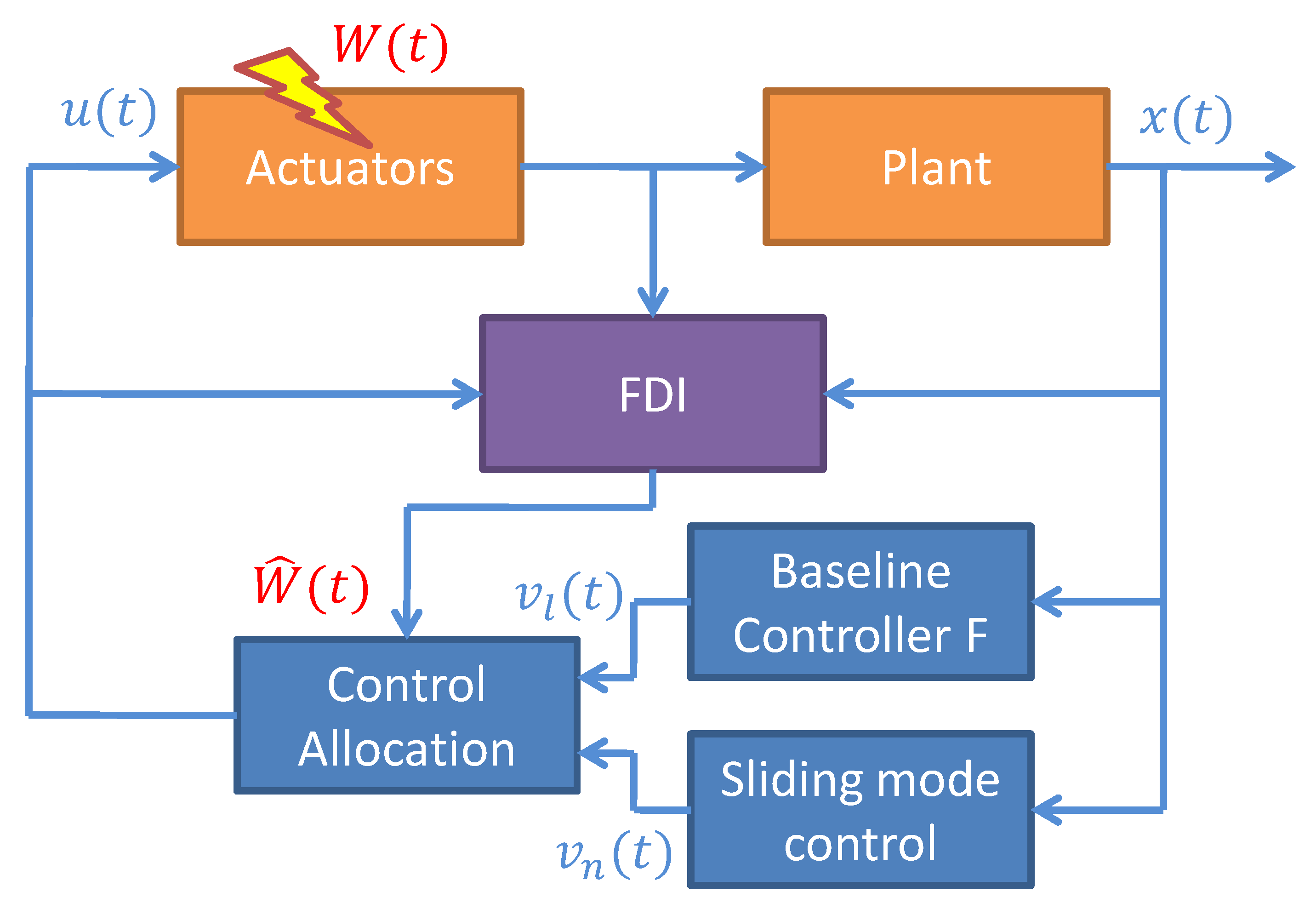
4.5. Sliding Mode Fault Tolerant Control
4.6. Fault Tolerant Control Based on Controller Reconfiguration
4.7. Fault-Hiding via Virtual Actuators and Virtual Sensors
5. Conclusions
Author Contributions
Funding
Conflicts of Interest
References
- Shamma, J.; Athans, M. Guaranteed properties for nonlinear gain scheduled control systems. In Proceedings of the 27th IEEE Conference on Decision and Control, Austin, TX, USA, 7–9 December 1988; Volume 3, pp. 2202–2208. [Google Scholar]
- Shamma, J.; Athans, M. Analysis of gain scheduled control for nonlinear plants. IEEE Trans. Autom. Control 1990, 35, 898–907. [Google Scholar] [CrossRef]
- Shamma, J. An Overview of LPV Systems. In Control of Linear Parameter Varying Systems with Applications; Mohammadpour, J., Scherer, C.W., Eds.; Springer: Boston, MA, USA, 2012; pp. 3–26. [Google Scholar]
- Tanaka, K.; Wang, H.O. Fuzzy Control Systems Design and Analysis: A Linear Matrix Inequality Approach; John Wiley & Sons: Hoboken, NJ, USA, 2004. [Google Scholar] [CrossRef]
- Jadbabaie, A.; Jamshidi, M.; Titli, A. Guaranteed-cost design of continuous-time Takagi-Sugeno fuzzy controllers via linear matrix inequalities. In Proceedings of the IEEE International Conference on Fuzzy Systems Proceedings, IEEE World Congress on Computational Intelligence, Anchorage, AK, USA, 4–9 May 1998; Volume 1, pp. 268–273. [Google Scholar]
- Ohtake, H.; Tanaka, K.; Wang, H.O. Fuzzy modeling via sector nonlinearity concept. Integr. Comput.-Aided Eng. 2003, 10, 333–341. [Google Scholar] [CrossRef]
- Ichalal, D.; Marx, B.; Ragot, J.; Maquin, D. State estimation of Takagi–Sugeno systems with unmeasurable premise variables. IET Control Theory Appl. 2010, 4, 897–908. [Google Scholar] [CrossRef]
- Lendek, Z.; Guerra, T.M.; Babuska, R.; De Schutter, B. Stability Analysis and Nonlinear Observer Design Using Takagi-Sugeno Fuzzy Models; Springer: Berlin/Heidelberg, Germany, 2011. [Google Scholar] [CrossRef]
- López-Estrada, F.R.; Astorga-Zaragoza, C.M.; Theilliol, D.; Ponsart, J.C.; Valencia-Palomo, G.; Torres, L. Observer synthesis for a class of Takagi–Sugeno descriptor system with unmeasurable premise variable. Application to fault diagnosis. Int. J. Syst. Sci. 2017, 48, 3419–3430. [Google Scholar] [CrossRef]
- Wang, Z.; Li, F.; Qin, Y.; Li, D.; Ma, G.; Ma, J. A Novel Dual Nonlinear Observer for Vehicle System Roll Behavior With Lateral and Vertical Coupling; SAE Technical Paper; SAE International: Warrendale, PA, USA, 2019. [Google Scholar] [CrossRef]
- Nagy Kiss, A.M.; Marx, B.; Mourot, G.; Schutz, G.; Ragot, J. State estimation of two-time scale multiple models. Application to wastewater treatment plant. Control Eng. Pract. 2011, 19, 1354–1362. [Google Scholar] [CrossRef]
- López-Estrada, F.R.; Ponsart, J.C.; Astorga-Zaragoza, C.M.; Camas-Anzueto, J.L.; Theilliol, D. Robust sensor fault estimation for descriptor-LPV systems with unmeasurable gain scheduling functions: Application to an anaerobic bioreactor. Int. J. Appl. Math. Comput. Sci. 2015, 25, 233–244. [Google Scholar] [CrossRef] [Green Version]
- Zhao, Z.; Wang, Y.; Liu, F. A multi-way LPV modeling method for batch processes. J. Process Control 2018, 65, 56–67. [Google Scholar] [CrossRef]
- Gómez-Peñate, S.; López-Estrada, F.R.; Valencia-Palomo, G.; Rotondo, D.; Enríquez-Zárate, J. Actuator and sensor fault estimation based on a proportional-integral quasi-LPV observer with inexact scheduling parameters. In Proceedings of the 3rd IFAC Workshop on Linear Parameter-Varying Systems, Eindhoven, The Netherlands, 4–6 November 2019. [Google Scholar]
- Lopez-Estrada, F.R.; Astorga-Zaragoza, C.M.; Valencia-Palomo, G.; Rios-Rojas, C.; Galicia-Gonzalez, C.; Escobar-Gomez, E. Observer-based LPV stabilization system for a riderless bicycle. IEEE Latin Am. Trans. 2018, 16, 1076–1083. [Google Scholar] [CrossRef]
- López-Estrada, F.R.; Theilliol, D.; Astorga-Zaragoza, C.M.; Ponsart, J.C.; Valencia-Palomo, G.; Camas Anzueto, J. Fault diagnosis observer for descriptor Takagi-Sugeno systems. Neurocomputing 2019, 331, 10–17. [Google Scholar] [CrossRef]
- Pfifer, H.; Moreno, C.P.; Theis, J.; Kotikapuldi, A.; Gupta, A.; Takarics, B.; Seiler, P. Linear parameter varying techniques applied to aeroservoelastic aircraft: In memory of Gary Balas. IFAC-PapersOnLine 2015, 48, 103–108. [Google Scholar] [CrossRef]
- Huang, B.; Lu, B.; Li, Q. A proportional–integral-based robust state-feedback control method for linear parameter-varying systems and its application to aircraft. Proc. Inst. Mech. Eng. Part G 2019, 233, 4663–4675. [Google Scholar] [CrossRef]
- Gutjahr, B.; Gröll, L.; Werling, M. Lateral vehicle trajectory optimization using constrained linear time-varying MPC. IEEE Trans. Intell. Transp. Syst. 2016, 18, 1586–1595. [Google Scholar] [CrossRef]
- Gómez-Peñate, S.; López-Estrada, F.R.; Valencia-Palomo, G.; Osornio-Ríos, R.; Zepeda-Hernández, J.; Rios-Rojas, C.; Camas-Anzueto, J. Sensor fault diagnosis observer for an electric vehicle modeled as a Takagi-Sugeno system. J. Sens. 2018, 2018, 3291639. [Google Scholar] [CrossRef]
- Chadli, M.; Borne, P. Multiple Models Approach in Automation: Takagi-Sugeno Fuzzy Systems; Wiley Online Library: London, UK, 2013. [Google Scholar] [CrossRef]
- Rotondo, D. Advances in Gain-Scheduling and Fault Tolerant Control Techniques; Springer: Cham, Switzerland, 2017. [Google Scholar] [CrossRef]
- Bernal, M.; Estrada, V.; Márquez, R. Diseño e Implementación de Sistemas de Control Basados en Estructuras Convexas Y Desigualdades Matriciales Lineales; Pearson: México city, Mexico, 2019. [Google Scholar]
- Rodrigues, M.; Hamdi, H.; BenHadj-Braiek, N.; Theilliol, D. Observer-based fault tolerant control design for a class of LPV descriptor systems. J. Frankl. Inst. 2014, 351, 3104–3125. [Google Scholar] [CrossRef] [Green Version]
- Rotondo, D.; Nejjari, F.; Puig, V. Quasi-LPV modeling, identification and control of a twin rotor MIMO system. Control Eng. Pract. 2013, 21, 829–846. [Google Scholar] [CrossRef]
- Rotondo, D.; Nejjari, F.; Puig, V. Robust quasi–LPV model reference FTC of a quadrotor UAV subject to actuator faults. Int. J. Appl. Math. Comput. Sci. 2015, 25, 7–22. [Google Scholar] [CrossRef]
- He, D.F.; Huang, H.; Chen, Q.X. Quasi-min–max MPC for constrained nonlinear systems with guaranteed input-to-state stability. J. Frankl. Inst. 2014, 351, 3405–3423. [Google Scholar] [CrossRef]
- He, Z.; Zhao, L. Quadrotor trajectory tracking based on quasi-LPV system and internal model control. Math. Probl. Eng. 2015, 2015, 857291. [Google Scholar] [CrossRef]
- Rizzello, G.; Naso, D.; Turchiano, B.; Seelecke, S. Robust position control of dielectric elastomer actuators based on LMI optimization. IEEE Trans. Control Syst. Technol. 2016, 24, 1909–1921. [Google Scholar] [CrossRef]
- Rizzello, G.; Ferrante, F.; Naso, D.; Seelecke, S. Robust interaction control of a dielectric elastomer actuator with variable stiffness. IEEE/ASME Trans. Mech. 2017, 22, 1705–1716. [Google Scholar] [CrossRef]
- Pérez-Estrada, A.J.; Osorio-Gordillo, G.L.; Darouach, M.; Alma, M.; Olivares-Peregrino, V.H. Generalized dynamic observers for quasi-LPV systems with unmeasurable scheduling functions. Int. J. Robust Nonlinear Control 2018, 28, 5262–5278. [Google Scholar] [CrossRef]
- Robles, R.; Sala, A.; Bernal, M. Performance-oriented quasi-LPV modeling of nonlinear systems. Int. J. Robust Nonlinear Control 2019, 29, 1230–1248. [Google Scholar] [CrossRef]
- Baranyi, P. Extracting LPV and qLPV structures from state-space functions: A TP model transformation based framework. IEEE Trans. Fuzzy Syst. 2019. [Google Scholar] [CrossRef]
- Rotondo, D.; Puig, V.; Nejjari, F.; Witczak, M. Automated generation and comparison of Takagi–Sugeno and polytopic quasi-LPV models. Fuzzy Sets Syst. 2015, 277, 44–64. [Google Scholar] [CrossRef]
- López-Estrada, F.R.; Ponsart, J.C.; Theilliol, D.; Zhang, Y.; Astorga-Zaragoza, C.M. LPV model-based tracking control and robust sensor fault diagnosis for a quadrotor UAV. J. Intell. Robot. Syst. 2016, 84, 163–177. [Google Scholar] [CrossRef]
- Ramírez, M.; Villafuerte, R.; González, T.; Bernal, M. Exponential estimates of a class of time–delay nonlinear systems with convex representations. Int. J. Appl. Math. Comput. Sci. 2015, 25, 815–826. [Google Scholar] [CrossRef]
- Arceo, J.C.; Vázquez, D.; Estrada-Manzo, V.; Márquez, R.; Bernal, M. Nonlinear convex control of the Furuta pendulum based on its descriptor model. In Proceedings of the 13th International Conference on Electrical Engineering, Computing Science and Automatic Control (CCE), Mexico City, Mexico, 26–30 September 2016; pp. 1–6. [Google Scholar]
- Quintana, D.; Estrada-Manzo, V.; Bernal, M. A methodology for real-time implementation of nonlinear observers via convex optimization. In Proceedings of the 15th International Conference on Electrical Engineering, Computing Science and Automatic Control (CCE), Mexico City, Mexico, 5–7 September 2018; pp. 1–6. [Google Scholar]
- Arceo, J.C.; Sánchez, M.; Estrada-Manzo, V.; Bernal, M. Convex stability analysis of nonlinear singular systems via linear matrix inequalities. IEEE Trans. Autom. Control 2018, 64, 1740–1745. [Google Scholar] [CrossRef]
- López-Estrada, F.R.; Hernández-de León, H.R.; Estrada-Manzo, V.; Bernal, M. LMI-based fault detection and isolation of nonlinear descriptor systems. In Proceedings of the IEEE International Conference on Fuzzy Systems (FUZZ-IEEE), Naples, Italy, 9–12 July 2017; pp. 1–5. [Google Scholar]
- Hoffmann, C.; Werner, H. A survey of linear parameter-varying control applications validated by experiments or high-fidelity simulations. IEEE Trans. Control Syst. Technol. 2014, 23, 416–433. [Google Scholar] [CrossRef]
- Apkarian, P.; Biannic, J.M.; Gahinet, P. Self-scheduled H∞ control of missile via linear matrix inequalities. J. Guid. Control Dyn. 1995, 18, 532–538. [Google Scholar] [CrossRef]
- Rugh, W.J.; Shamma, J.S. Research on gain scheduling. Automatica 2000, 36, 1401–1425. [Google Scholar] [CrossRef]
- Shamma, J.S.; Athans, M. Gain scheduling: Potential hazards and possible remedies. IEEE Control Syst. Mag. 1992, 12, 101–107. [Google Scholar]
- Rotondo, D.; Nejjari, F.; Puig, V. Robust state-feedback control of uncertain LPV systems: An LMI-based approach. J. Frankl. Inst. 2014, 351, 2781–2803. [Google Scholar] [CrossRef]
- Sato, M. Gain-scheduled output-feedback controllers depending solely on scheduling parameters via parameter-dependent Lyapunov functions. Automatica 2011, 47, 2786–2790. [Google Scholar] [CrossRef]
- Sato, M.; Peaucelle, D. Gain-scheduled output-feedback controllers using inexact scheduling parameters for continuous-time LPV systems. Automatica 2013, 49, 1019–1025. [Google Scholar] [CrossRef]
- Kajiwara, H.; Apkarian, P.; Gahinet, P. LPV Techniques for Control of an Inverted Pendulum. IEEE Control Syst. 1999, 19, 44–54. [Google Scholar]
- Bruzelius, F.; Breitholtz, C.; Pettersson, S. LPV-based gain scheduling technique applied to a turbo fan engine model. In Proceedings of the International Conference on Control Applications, Glasgow, UK, 18–20 September 2002; pp. 713–718. [Google Scholar]
- Scherer, C.W. Robust Mixed Control and LPV Control with Full Block Scaling; Technical Report; Delft University of Technology, Mechanical Engineering Systems and Control Group: Delft, The Netherlands, 2004. [Google Scholar]
- Mohammadpour, J.; Scherer, C. Control of Linear Parameter Varying Systems with Applications; Springer: New York, NY, USA, 2012. [Google Scholar] [CrossRef]
- Xu, H.E.; Jun, Z.; M, D.G.; Chao, C. Switching control for LPV polytopic systems using multiple Lyapunov functions. In Proceedings of the 30th Chinese Control Conference, Yantai, China, 22–24 July 2011; pp. 1771–1776. [Google Scholar]
- Xu, H.E.; Jun, Z.; Dimirovski, G.M. A blending method control of switched LPV systems with slow-varying parameters and its application to an F-16 aircraft model. In Proceedings of the 30th Chinese Control Conference, Yantai, China, 22–24 July 2011; pp. 1765–1770. [Google Scholar]
- Shin, J.; Balas, G.; Kaya, A.M. Blending methodology of linear parameter varying control synthesis of F-16 aircraft system. J. Guid. Control Dyn. 2002, 25, 1040–1048. [Google Scholar] [CrossRef]
- Xie, W.; Kamiya, Y.; Eisaka, T. Robust control system design for polytopic stable LPV systems. IMA J. Math. Control Inf. 2003, 20, 201–216. [Google Scholar] [CrossRef]
- Qiu, J.; Feng, G.; Gao, H. Fuzzy-Model-Based Piecewise H∞ Static-Output-Feedback Controller Design for Networked Nonlinear Systems. IEEE Trans. Fuzzy Syst. 2010, 18, 919–934. [Google Scholar] [CrossRef]
- Yin, X.; Zhang, L.; Zhu, Y.; Wang, C.; Li, Z. Robust control of networked systems with variable communication capabilities and application to a semi-active suspension system. IEEE/ASME Trans. Mech. 2016, 21, 2097–2107. [Google Scholar] [CrossRef]
- Shamma, J.S. Analysis and Design of Gain Scheduled Control Systems. Ph.D. Thesis, Massachusetts Institute of Technology, Cambridge, MA, USA, 1988. [Google Scholar]
- Shamma, J.S.; Athans, M. Guaranteed properties of gain scheduled control for linear parameter-varying plants. Automatica 1991, 27, 559–564. [Google Scholar] [CrossRef]
- Goebel, R.; Hu, T.; Teel, A.R. Dual matrix inequalities in stability and performance analysis of linear differential/difference inclusions. In Current Trends in Nonlinear Systems and Control; Springer: Boston, MA, USA, 2006; pp. 103–122. [Google Scholar] [CrossRef]
- Apkarian, P.; Gahinet, P.; Becker, G. Self-scheduled H∞ control of linear parameter-varying systems: A design example. Automatica 1995, 31, 1251–1261. [Google Scholar] [CrossRef]
- Pandey, A.; Sehr, M.; de Oliveira, M. Pre-filtering in gain-scheduled and robust control. In Proceedings of the American Control Conference (ACC), Boston, MA, USA, 6–8 July 2016; pp. 3698–3703. [Google Scholar]
- Sehr, M.A.; de Oliveira, M.C. Pre-filtering and post-filtering in gain-scheduled output-feedback control. Int. J. Robust Nonlinear Control 2017, 27, 3259–3279. [Google Scholar] [CrossRef]
- Sala, A.; Arino, C. Asymptotically necessary and sufficient conditions for stability and performance in fuzzy control: Applications of Polya’s theorem. Fuzzy Sets Syst. 2007, 158, 2671–2686. [Google Scholar] [CrossRef]
- Kruszewski, A.; Sala, A.; Guerra, T.M.; Ariño, C. A triangulation approach to asymptotically exact conditions for fuzzy summations. IEEE Trans. Fuzzy Syst. 2009, 17, 985–994. [Google Scholar] [CrossRef]
- Sala, A.; Arino, C. Relaxed stability and performance LMI conditions for Takagi–Sugeno fuzzy systems with polynomial constraints on membership function shapes. IEEE Trans. Fuzzy Syst. 2008, 16, 1328–1336. [Google Scholar] [CrossRef]
- Tuan, H.D.; Apkarian, P.; Narikiyo, T.; Yamamoto, Y. Parameterized linear matrix inequality techniques in fuzzy control system design. IEEE Trans. Fuzzy Syst. 2001, 9, 324–332. [Google Scholar] [CrossRef]
- Wang, H.O.; Tanaka, K.; Griffin, M. Parallel distributed compensation of nonlinear systems by Takagi-Sugeno fuzzy model. In Proceedings of the 1995 IEEE International Conference on Fuzzy Systems, Yokohama, Japan, 20–24 March 1995; Volume 2, pp. 531–538. [Google Scholar]
- Wang, L.K.; Zhang, H.G.; Liu, X.D. H∞ Observer Design for Continuous-Time Takagi-Sugeno Fuzzy Model with Unknown Premise Variables via Nonquadratic Lyapunov Function. IEEE Trans. Cybern. 2016, 46, 1986–1996. [Google Scholar] [CrossRef]
- Márquez, R.; Guerra, T.M.; Bernal, M.; Kruszewski, A. A non-quadratic Lyapunov functional for H∞ control of nonlinear systems via Takagi-Sugeno models. J. Frankl. Inst. 2016, 353, 781–796. [Google Scholar] [CrossRef]
- Márquez, R.; Guerra, T.M.; Bernal, M.; Kruszewski, A. Asymptotically necessary and sufficient conditions for Takagi–Sugeno models using generalized non-quadratic parameter-dependent controller design. Fuzzy Sets Syst. 2017, 306, 48–62. [Google Scholar] [CrossRef]
- Pandey, A.; de Oliveira, M.C. Quadratic and poly-quadratic discrete-time stabilizability of linear parameter-varying systems. IFAC-PapersOnLine 2017, 50, 8624–8629. [Google Scholar] [CrossRef]
- Lam, H.K.; Wu, L.; Zhao, Y. Linear matrix inequalities-based membership-function-dependent stability analysis for non-parallel distributed compensation fuzzy-model-based control systems. IET Control Theory Appl. 2014, 8, 614–625. [Google Scholar] [CrossRef]
- Cherifi, A.; Guelton, K.; Arcese, L. Quadratic design of d-stabilizing non-pdc controllers for quasi-lpv/ts models. IFAC-PapersOnLine 2015, 48, 164–169. [Google Scholar] [CrossRef]
- Guerra, T.M.; Bernal, M.; Guelton, K.; Labiod, S. Non-quadratic local stabilization for continuous-time Takagi–Sugeno models. Fuzzy Sets Syst. 2012, 201, 40–54. [Google Scholar] [CrossRef]
- Daafouz, J.; Bernussou, J. Parameter dependent Lyapunov functions for discrete time systems with time varying parametric uncertainties. Syst. Control Lett. 2001, 43, 355–359. [Google Scholar] [CrossRef]
- Chadli, M.; Daafouz, J.; Darouach, M. Stabilisation of singular LPV systems. IFAC Proc. Vol. 2008, 41, 9999–10002. [Google Scholar] [CrossRef]
- Pandey, A.P.; de Oliveira, M.C. On the necessity of LMI-based design conditions for discrete time LPV filters. IEEE Trans. Autom. Control 2018, 63, 3187–3188. [Google Scholar] [CrossRef]
- El Ghaoui, L.; Oustry, F.; AitRami, M. A cone complementarity linearization algorithm for static output-feedback and related problems. IEEE Trans. Autom. Control 1997, 42, 1171–1176. [Google Scholar] [CrossRef]
- Prempain, E.; Postlethwaite, I. Static H∞ loop shaping control of a fly-by-wire helicopter. Automatica 2005, 41, 1517–1528. [Google Scholar] [CrossRef]
- Henrion, D.; Lasserre, J.B. Convergent relaxations of polynomial matrix inequalities and static output feedback. IEEE Trans. Autom. Control 2006, 51, 192–202. [Google Scholar] [CrossRef]
- Apkarian, P.; Noll, D. Nonsmooth H∞ synthesis. IEEE Trans. Autom. Control 2006, 51, 71–86. [Google Scholar] [CrossRef]
- Scherer, C.; Gahinet, P.; Chilali, M. H∞ design with pole placement constraints: An LMI approach. IEEE Trans. Autom. Control 1996, 41, 358–367. [Google Scholar]
- Gahinet, P. Explicit controller formulas for LMI-based H∞ synthesis. Automatica 1996, 32, 1007–1014. [Google Scholar] [CrossRef]
- Amato, F. Robust Control of Linear Systems Subject to Uncertain Time-Varying Parameters; Springer: Berlin/Heidelberg, Germany, 2006; Volume 325. [Google Scholar] [CrossRef]
- Kose, I.E.; Jabbari, F. Control of LPV systems with partly measured parameters. IEEE Trans. Autom. Control 1999, 44, 658–663. [Google Scholar] [CrossRef]
- Abdullah, A.; Zribi, M. Model reference control of LPV systems. J. Frankl. Inst. 2009, 346, 854–871. [Google Scholar] [CrossRef]
- Rotondo, D.; Puig, V.; Nejjari, F.; Romera, J. A fault-hiding approach for the switching quasi-LPV fault-tolerant control of a four-wheeled omnidirectional mobile robot. IEEE Trans. Ind. Electron. 2014, 62, 3932–3944. [Google Scholar] [CrossRef]
- Valencia-Palomo, G.; Rossiter, J.A. Auto-tuned predictive control based on minimal plant information. IFAC Proc. Vol. 2009, 42, 554–559. [Google Scholar] [CrossRef]
- Valencia-Palomo, G.; Rossiter, J.; López-Estrada, F. Improving the feed-forward compensator in predictive control for setpoint tracking. ISA Trans. 2014, 53, 755–766. [Google Scholar] [CrossRef] [PubMed]
- Valencia-Palomo, G.; Hilton, K.; Rossiter, J.A. Predictive control implementation in a PLC using the IEC 1131.3 programming standard. In Proceedings of the 2009 European Control Conference (ECC), Budapest, Hungary, 23–26 August 2009; pp. 1317–1322. [Google Scholar]
- Kothare, M.V.; Balakrishnan, V.; Morari, M. Robust constrained model predictive control using linear matrix inequalities. Automatica 1996, 32, 1361–1379. [Google Scholar] [CrossRef] [Green Version]
- Lu, Y.; Arkun, Y. Quasi-min-max MPC algorithms for LPV systems. Automatica 2000, 36, 527–540. [Google Scholar] [CrossRef]
- Park, P.; Jeong, S.C. Constrained RHC for LPV systems with bounded rates of parameter variations. Automatica 2004, 40, 865–872. [Google Scholar] [CrossRef]
- Lu, Y.; Arkun, Y. Polytope updating in quasi-min-max MPC algorithms. IFAC Proc. Vol. 2000, 33, 407–412. [Google Scholar] [CrossRef]
- Lu, Y.; Arkun, Y. A scheduling quasi–min-max model predictive control algorithm for nonlinear systems. J. Process Control 2002, 12, 589–604. [Google Scholar] [CrossRef]
- Lee, S.; Won, S. Model predictive control for linear parameter varying systems using a new parameter dependent terminal weighting matrix. IEICE Trans. Fund. Electron. Commun. Comput. Sci. 2006, 89, 2166–2172. [Google Scholar] [CrossRef]
- Wada, N.; Saito, K.; Saeki, M. Model predictive control for linear parameter varying systems using parameter dependent Lyapunov function. IEEE Trans. Circuits Syst. II 2006, 12, 1446–1450. [Google Scholar] [CrossRef]
- Pluymers, B.; Rossiter, J.; Suykens, J.; De Moor, B. The efficient computation of polyhedral invariant sets for linear systems with polytopic uncertainty. In Proceedings of the American Control Conference, Portland, OR, USA, 8–10 June 2005; pp. 804–809. [Google Scholar] [CrossRef]
- Garone, E.; Casavola, A. Receding horizon control strategies for constrained LPV systems based on a class of nonlinearly parameterized Lyapunov functions. IEEE Trans. Autom. Control 2012, 57, 2354–2360. [Google Scholar] [CrossRef]
- Yu, S.; Böhm, C.; Chen, H.; Allgöwer, F. Model predictive control of constrained LPV systems. Int. J. Control 2012, 85, 671–683. [Google Scholar] [CrossRef]
- Besselmann, T.; Lofberg, J.; Morari, M. Explicit MPC for LPV systems: Stability and optimality. IEEE Trans. Autom. Control 2012, 57, 2322–2332. [Google Scholar] [CrossRef]
- Zhang, J.; Xiu, X. Kd tree based approach for point location problem in explicit model predictive control. J. Frankl. Inst. 2018, 355, 5431–5451. [Google Scholar] [CrossRef]
- Ariño, C.; Querol, A.; Sala, A. Shape-independent model predictive control for Takagi–Sugeno fuzzy systems. Eng. Appl. Artif. Intell. 2017, 65, 493–505. [Google Scholar] [CrossRef]
- Hanema, J.; Lazar, M.; Tóth, R. Stabilizing tube-based model predictive control: Terminal set and cost construction for LPV systems. Automatica 2017, 85, 137–144. [Google Scholar] [CrossRef]
- Ding, B.; Wang, P.; Hu, J. Dynamic output feedback robust MPC with one free control move for LPV model with bounded disturbance. Asian J. Control 2018, 20, 755–767. [Google Scholar] [CrossRef]
- Morato, M.M.; Nguyen, M.Q.; Sename, O.; Dugard, L. Design of a fast real-time LPV model predictive control system for semi-active suspension control of a full vehicle. J. Frankl. Inst. 2019, 356, 1196–1224. [Google Scholar] [CrossRef]
- Ghersin, A.S.; Pena, R.S.S. Applied LPV control with full block multipliers and regional pole placement. J. Control Sci. Eng. 2010, 2010, 3. [Google Scholar] [CrossRef]
- Ostertag, E. Mono-and Multivariable Control and Estimation: Linear, Quadratic and LMI Methods; Springer: Berlin/Heidelberg, Germany, 2011. [Google Scholar] [CrossRef]
- Rotondo, D.; Puig, V.; Nejjari, F. Linear quadratic control of LPV systems using static and shifting specifications. In Proceedings of the European Control Conference (ECC), Linz, Austria, 15–17 July 2015; pp. 3085–3090. [Google Scholar]
- Briat, C. Stability analysis and control of a class of LPV systems with piecewise constant parameters. Syst. Control Lett. 2015, 82, 10–17. [Google Scholar] [CrossRef]
- Bruzelius, F.; Pettersson, S.; Breitholtz, C. Region of attraction estimates for LPV-gain scheduled control systems. In Proceedings of the European Control Conference (ECC), Cambridge, UK, 1–4 September 2003; pp. 892–897. [Google Scholar] [CrossRef]
- Pitarch, J.L.; Sala, A.; Arino, C.V. Closed-form estimates of the domain of attraction for nonlinear systems via fuzzy-polynomial models. IEEE Trans. Cybern. 2013, 44, 526–538. [Google Scholar] [CrossRef]
- Lendek, Z.; Lauber, J. Local stability of discrete-time TS fuzzy systems. IFAC-PapersOnLine 2016, 49, 7–12. [Google Scholar] [CrossRef]
- Lendek, Z.; Nagy, Z.; Lauber, J. Local stabilization of discrete-time TS descriptor systems. Eng. Appl. Artif. Intell. 2018, 67, 409–418. [Google Scholar] [CrossRef]
- Zhang, X.; Tsiotras, P.; Knospe, C. Stability analysis of LPV time-delayed systems. Int. J. Control 2002, 75, 538–558. [Google Scholar] [CrossRef]
- Wu, F.; Grigoriadis, K.M. LPV systems with parameter-varying time delays: Analysis and control. Automatica 2001, 37, 221–229. [Google Scholar] [CrossRef]
- Briat, C.; Sename, O.; Lafay, J.F. Memory-resilient gain-scheduled state-feedback control of uncertain LTI/LPV systems with time-varying delays. Syst. Control Lett. 2010, 59, 451–459. [Google Scholar] [CrossRef] [Green Version]
- Briat, C. Linear Parameter-Varying and Time-Delay Systems: Analysis, Observation, Filtering Control; Springer: Berlin/Heidelberg, Germany, 2014; Volume 3. [Google Scholar] [CrossRef]
- Guzmán-Rabasa, J.A.; López-Estrada, F.R.; González-Contreras, B.M.; Valencia-Palomo, G.; Chadli, M.; Pérez-Patricio, M. Actuator fault detection and isolation on a quadrotor unmanned aerial vehicle modeled as a linear parameter-varying system. Meas. Control 2019. [Google Scholar] [CrossRef]
- Zhang, H.; Zhang, G.; Wang, J. H∞ Observer Design for LPV Systems With Uncertain Measurements on Scheduling Variables: Application to an Electric Ground Vehicle. IEEE/ASME Trans. Mech. 2016, 21, 1659–1670. [Google Scholar] [CrossRef]
- Li, H.; Wu, C.; Yin, S.; Lam, H.K. Observer-based fuzzy control for nonlinear networked systems under unmeasurable premise variables. IEEE Trans. Fuzzy Syst. 2015, 24, 1233–1245. [Google Scholar] [CrossRef]
- Ibrir, S.; Sabir, A. Robust observer-based stabilization and tracking of uncertain linear systems with L2-gain performance: Application to DC motors. In Proceedings of the 2016 IEEE International Energy Conference (ENERGYCON), Leuven, Belgium, 4–8 April 2016; pp. 1–6. [Google Scholar] [CrossRef]
- Gauterin, E.; Kammerer, P.; Kühn, M.; Schulte, H. Effective wind speed estimation: Comparison between Kalman Filter and Takagi–Sugeno observer techniques. ISA Trans. 2016, 62, 60–72. [Google Scholar] [CrossRef]
- Brizuela-Mendoza, J.A.; Astorga-Zaragoza, C.M.; Zavala-Río, A.; Pattalochi, L.; Canales-Abarca, F. State and actuator fault estimation observer design integrated in a riderless bicycle stabilization system. ISA Trans. 2016, 61, 199–210. [Google Scholar] [CrossRef]
- Bergsten, P.; Palm, R.; Driankov, D. Observers for Takagi-Sugeno fuzzy systems. IEEE Trans. Syst. Man Cybern. Part B 2002, 32, 114–121. [Google Scholar] [CrossRef]
- Zhang, L.; Yin, X.; Ning, Z.; Ye, D. Robust filtering for a class of networked nonlinear systems with switching communication channels. IEEE Trans. Cybern. 2016, 47, 671–682. [Google Scholar] [CrossRef]
- Gómez-Peñate, S.; Valencia-Palomo, G.; López-Estrada, F.R.; Astorga-Zaragoza, C.M.; Osornio-Rios, R.A.; Santos-Ruiz, I. Sensor fault diagnosis based on a sliding mode and unknown input observer for Takagi-Sugeno systems with uncertain premise variables. Asian J. Control 2019, 21, 339–353. [Google Scholar] [CrossRef]
- Busawon, K.K.; Kabore, P. Disturbance attenuation using proportional integral observers. Int. J. Control 2001, 74, 618–627. [Google Scholar] [CrossRef]
- Youssef, T.; Chadli, M.; Karimi, H.R.; Zelmat, M. Design of unknown inputs proportional integral observers for TS fuzzy models. Neurocomputing 2014, 123, 156–165. [Google Scholar] [CrossRef]
- Kang, D. Design of a disturbance observer for discrete-time linear systems. In Proceedings of the 14th International Conference on Control, Automation and Systems (ICCAS), Seoul, South Korea, 22–25 October 2014; pp. 1381–1383. [Google Scholar]
- Xu, J.; Mi, C.C.; Cao, B.; Deng, J.; Chen, Z.; Li, S. The state of charge estimation of lithium-ion batteries based on a proportional-integral observer. IEEE Trans. Veh. Technol. 2013, 63, 1614–1621. [Google Scholar]
- Youssef, T.; Chadli, M.; Karimi, H.R.; Wang, R. Actuator and sensor faults estimation based on proportional integral observer for TS fuzzy model. J. Frankl. Inst. 2017, 354, 2524–2542. [Google Scholar] [CrossRef]
- Rotondo, D.; Cristofaro, A.; Johansen, T.A.; Nejjari, F.; Puig, V. Detection of icing and actuators faults in the longitudinal dynamics of small UAVs using an LPV proportional integral unknown input observer. In Proceedings of the 3rd Conference on Control and Fault-Tolerant Systems (SysTol), Barcelona, Spain, 7–9 Deptember 2016; pp. 690–697. [Google Scholar] [CrossRef]
- Rotondo, D.; López-Estrada, F.R.; Nejjari, F.; Ponsart, J.C.; Theilliol, D.; Puig, V. Actuator multiplicative fault estimation in discrete-time LPV systems using switched observers. J. Frankl. Inst. 2016, 353, 3176–3191. [Google Scholar] [CrossRef] [Green Version]
- Duan, G.R. Analysis and Design of Descriptor Linear Systems; Springer: New York, NY, USA, 2010. [Google Scholar] [CrossRef]
- Masubuchi, I.; Kato, J.; Saeki, M.; Ohara, A. Gain-scheduled controller design based on descriptor representation of LPV systems: Application to flight vehicle control. In Proceedings of the 43rd IEEE Conference on Decision and Control (CDC), Nassau, Bahamas, 14–17 December 2004; Volume 1, pp. 815–820. [Google Scholar]
- Baghaee, H.R.; Mirsalim, M.; Gharehpetian, G.B.; Talebi, H.A. A generalized descriptor-system robust H∞ control of autonomous microgrids to improve small and large signal stability considering communication delays and load nonlinearities. Int. J. Electr. Power Energy Syst. 2017, 92, 63–82. [Google Scholar] [CrossRef]
- González, A.; Estrada-Manzo, V.; Guerra, T.M. Gain-scheduled H∞ admissibilisation of LPV discrete-time systems with LPV singular descriptor. Int. J. Syst. Sci. 2017, 48, 3215–3224. [Google Scholar] [CrossRef]
- Arceo, J.C.; Villafuerte, R.; Estrada-Manzo, V.; Bernal, M. LMI-Based Controller Design for Time-Delay Nonlinear Descriptor Systems with Guaranteed Exponential Estimates. IFAC-PapersOnLine 2018, 51, 585–590. [Google Scholar] [CrossRef]
- González, A.; Guerra, T.M. Enhanced Predictor-Based Control Synthesis for Discrete-Time TS Fuzzy Descriptor Systems With Time-Varying Input Delays. IEEE Trans. Fuzzy Syst. 2018, 27, 402–410. [Google Scholar] [CrossRef]
- Guerra, T.M.; Estrada-Manzo, V.; Lendek, Z. Observer design for Takagi–Sugeno descriptor models: An LMI approach. Automatica 2015, 52, 154–159. [Google Scholar] [CrossRef]
- Estrada-Manzo, V.; Lendek, Z.; Guerra, T.M. Generalized LMI observer design for discrete-time nonlinear descriptor models. Neurocomputing 2016, 182, 210–220. [Google Scholar] [CrossRef]
- Hamdi, H.; Rodrigues, M.; Mechmeche, C.; Theilliol, D. Fault detection and isolation for linear parameter varying descriptor systems via proportional integral observer. Int. J. Adapt. Control Signal Proc. 2012, 26, 224–240. [Google Scholar] [CrossRef]
- Alwi, H.; Edwards, C. Fault tolerant longitudinal aircraft control using non-linear integral sliding mode. IET Control Theory Appl. 2014, 8, 1803–1814. [Google Scholar] [CrossRef]
- Gertler, J. Fault Detection and Diagnosis; John Wiley & Sons, Ltd.: Hoboken, NJ, USA, 2008. [Google Scholar] [CrossRef]
- Wei, X.; Verhaegen, M. LMI solutions to the mixed H∞/H_ fault detection observer design for linear parameter-varying systems. Int. J. Adapt. Control Signal Proc. 2011, 25, 114–136. [Google Scholar] [CrossRef]
- Chadli, M.; Abdo, A.; Ding, S.X. H_/H∞ fault detection filter design for discrete-time Takagi-Sugeno fuzzy system. Automatica 2013, 49, 1996–2005. [Google Scholar] [CrossRef]
- Chibani, A.; Chadli, M.; Shi, P.; Braiek, N.B. Fuzzy fault detection filter design for T–S fuzzy systems in the finite-frequency domain. IEEE Trans. Fuzzy Syst. 2016, 25, 1051–1061. [Google Scholar] [CrossRef]
- Wang, Z.; Shi, P.; Lim, C.C. H_/H∞ fault detection observer in finite frequency domain for linear parameter-varying descriptor systems. Automatica 2017, 86, 38–45. [Google Scholar] [CrossRef]
- Chibani, A.; Chadli, M.; Ding, S.X.; Braiek, N.B. Design of robust fuzzy fault detection filter for polynomial fuzzy systems with new finite frequency specifications. Automatica 2018, 93, 42–54. [Google Scholar] [CrossRef]
- Iwasaki, T.; Hara, S. Generalized KYP lemma: Unified frequency domain inequalities with design applications. IEEE Trans. Autom. Control 2005, 50, 41–59. [Google Scholar] [CrossRef]
- Estrada, F.L.; Ponsart, J.C.; Theilliol, D.; Astorga-Zaragoza, C.M. Robust H_/H∞ fault detection observer design for descriptor-LPV systems with unmeasurable gain scheduling functions. Int. J. Control 2015, 88, 2380–2391. [Google Scholar] [CrossRef]
- Darouach, M.; Zasadzinski, M.; Xu, S.J. Full-order observers for linear systems with unknown inputs. IEEE Trans. Autom. Control 1994, 39, 606–609. [Google Scholar] [CrossRef] [Green Version]
- Rotondo, D.; Witczak, M.; Puig, V.; Nejjari, F.; Pazera, M. Robust unknown input observer for state and fault estimation in discrete-time Takagi–Sugeno systems. Int. J. Syst. Sci. 2016, 47, 3409–3424. [Google Scholar] [CrossRef]
- Rotondo, D.; Cristofaro, A.; Johansen, T.A.; Nejjari, F.; Puig, V. Icing detection in unmanned aerial vehicles with longitudinal motion using an LPV unknown input observer. In Proceedings of the Conference on Control Applications (CCA), Sydney, Australia, 21–23 September 2015; pp. 984–989. [Google Scholar] [CrossRef]
- Chadli, M.; Karimi, H.R. Robust observer design for unknown inputs Takagi–Sugeno models. IEEE Trans. Fuzzy Syst. 2012, 21, 158–164. [Google Scholar] [CrossRef]
- Meyer, L.; Ichalal, D.; Vigneron, V. Interval observer for LPV systems with unknown inputs. IET Control Theory Appl. 2017, 12, 649–660. [Google Scholar] [CrossRef]
- Rotondo, D.; Cristofaro, A.; Johansen, T.A.; Nejjari, F.; Puig, V. State estimation and decoupling of unknown inputs in uncertain LPV systems using interval observers. Int. J. Control 2018, 91, 1944–1961. [Google Scholar] [CrossRef]
- Rotondo, D.; Cristofaro, A.; Johansen, T.A.; Nejjari, F.; Puig, V. Robust fault and icing diagnosis in unmanned aerial vehicles using LPV interval observers. Int. J. Robust Nonlinear Control 2018. [Google Scholar] [CrossRef]
- Hassanabadi, A.H.; Shafiee, M.; Puig, V. Actuator fault diagnosis of singular delayed LPV systems with inexact measured parameters via PI unknown input observer. IET Control Theory Appl. 2017, 11, 1894–1903. [Google Scholar] [CrossRef]
- Xu, F.; Tan, J.; Wang, Y.; Wang, X.; Liang, B.; Yuan, B. Robust fault detection and set-theoretic UIO for discrete-time LPV systems with state and output equations scheduled by inexact scheduling variables. IEEE Trans. Autom. Control 2019. [Google Scholar] [CrossRef]
- Marx, B.; Ichalal, D.; Ragot, J.; Maquin, D.; Mammar, S. Unknown input observer for LPV systems. Automatica 2019, 100, 67–74. [Google Scholar] [CrossRef]
- Rodrigues, M.; Hamdi, H.; Theilliol, D.; Mechmeche, C.; BenHadj Braiek, N. Actuator fault estimation based adaptive polytopic observer for a class of LPV descriptor systems. Int. J. Robust Nonlinear Control 2015, 25, 673–688. [Google Scholar] [CrossRef]
- Chandra, K.P.B.; Alwi, H.; Edwards, C. Fault detection in uncertain LPV systems with imperfect scheduling parameter using sliding mode observers. Eur. J. Control 2017, 34, 1–15. [Google Scholar] [CrossRef] [Green Version]
- Chen, L.; Edwards, C.; Alwi, H. Sensor fault estimation using LPV sliding mode observers with erroneous scheduling parameters. Automatica 2019, 101, 66–77. [Google Scholar] [CrossRef]
- Zhang, K.; Jiang, B.; Shi, P.; Xu, J. Analysis and design of robust H_/H∞ fault estimation observer with finite-frequency specifications for discrete-time fuzzy systems. IEEE Trans. Cybern. 2014, 45, 1225–1235. [Google Scholar] [CrossRef] [PubMed]
- Xie, X.; Yue, D.; Zhang, H.; Xue, Y. Fault estimation observer design for discrete-time Takagi–Sugeno fuzzy systems based on homogenous polynomially parameter-dependent Lyapunov functions. IEEE Trans. Cybern. 2017, 47, 2504–2513. [Google Scholar] [CrossRef] [PubMed]
- Lopez-Estrada, F.R.; Ponsart, J.C.; Theilliol, D.; Astorga-Zaragoza, C.; Flores-Montiel, M. Robust state and fault estimation observer for discrete-time D-LPV systems with unmeasurable gain scheduling functions. Application to a binary distillation column. IFAC-PapersOnLine 2015, 48, 1012–1017. [Google Scholar] [CrossRef]
- Morato, M.M.; Sename, O.; Dugard, L.; Nguyen, M.Q. Fault estimation for automotive Electro-Rheological dampers: LPV-based observer approach. Control Eng. Pract. 2019, 85, 11–22. [Google Scholar] [CrossRef] [Green Version]
- Morato, M.M.; Mendes, P.R.; Normey-Rico, J.E.; Bordons, C. Robustness conditions of LPV fault estimation systems for renewable microgrids. Int. J. Electr. Power Energy Syst. 2019, 111, 325–350. [Google Scholar] [CrossRef]
- Morato, M.M.; Regner, D.J.; Mendes, P.R.; Normey-Rico, J.E.; Bordons, C. Fault analysis, detection and estimation for a microgrid via H2/H∞ LPV observers. Int. J. Electr. Power Energy Syst. 2019, 105, 823–845. [Google Scholar] [CrossRef]
- Li, X.R.; Bar-Shalom, Y. Multiple-model estimation with variable structure. IEEE Trans. Autom. Control 1996, 41, 478–493. [Google Scholar]
- Hassani, V.; Aguiar, A.P.; Athans, M.; Pascoal, A.M. Multiple model adaptive estimation and model identification usign a minimum energy criterion. In Proceedings of the American Control Conference (ACC), St. Louis, MO, USA, 10–12 June 2009; pp. 518–523. [Google Scholar] [CrossRef]
- Xiong, K.; Wei, C.; Liu, L. Robust multiple model adaptive estimation for spacecraft autonomous navigation. Aerosp. Sci. Technol. 2015, 42, 249–258. [Google Scholar] [CrossRef]
- Rotondo, D.; Hassani, V.; Cristofaro, A. A multiple model adaptive architecture for the state estimation in discrete-time uncertain LPV systems. In Proceedings of the American Control Conference (ACC), Seattle, WA, USA, 24–26 May 2017; pp. 2393–2398. [Google Scholar]
- Rotondo, D.; Cristofaro, A.; Hassani, V.; Johansen, T.A. Icing diagnosis in unmanned aerial vehicles using an LPV multiple model estimator. IFAC-PapersOnLine 2017, 50, 5238–5243. [Google Scholar] [CrossRef]
- Yang, G.H.; Wang, H. Fault detection and isolation for a class of uncertain state-feedback fuzzy control systems. IEEE Trans. Fuzzy Syst. 2014, 23, 139–151. [Google Scholar] [CrossRef]
- Alwi, H.; Edwards, C.; Tan, C.P. Fault Detection and Fault-Tolerant Control Using Sliding Modes; Springer: London, UK, 2011. [Google Scholar] [CrossRef]
- Sivrioglu, S.; Nonami, K. Sliding mode control with time-varying hyperplane for AMB systems. IEEE/ASME Trans. Mech. 1998, 3, 51–59. [Google Scholar] [CrossRef]
- Alwi, H.; Edwards, C.; Stroosma, O.; Mulder, J.; Hamayun, M.T. Real-time implementation of an ISM fault-tolerant control scheme for LPV plants. IEEE Trans. Ind. Electron. 2014, 62, 3896–3905. [Google Scholar]
- Hamayun, M.T.; Ijaz, S.; Bajodah, A.H. Output integral sliding mode fault tolerant control scheme for LPV plants by incorporating control allocation. IET Control Theory Appl. 2017, 11, 1959–1967. [Google Scholar] [CrossRef]
- Selvaraj, P.; Kaviarasan, B.; Sakthivel, R.; Karimi, H.R. Fault-tolerant SMC for Takagi–Sugeno fuzzy systems with time-varying delay and actuator saturation. IET Control Theory Appl. 2017, 11, 1112–1123. [Google Scholar] [CrossRef]
- Shin, J.Y.; Wu, N.E.; Belcastro, C. Adaptive linear parameter varying control synthesis for actuator failure. J. Guid. Control Dyn. 2004, 27, 787–794. [Google Scholar] [CrossRef]
- Sloth, C.; Esbensen, T.; Stoustrup, J. Robust and fault-tolerant linear parameter-varying control of wind turbines. Mechatronics 2011, 21, 645–659. [Google Scholar] [CrossRef] [Green Version]
- Jia, Q.; Chen, W.; Zhang, Y.; Li, H. Fault reconstruction and fault-tolerant control via learning observers in Takagi–Sugeno fuzzy descriptor systems with time delays. IEEE Trans. Ind. Electron. 2015, 62, 3885–3895. [Google Scholar] [CrossRef]
- Li, X.; Zhu, F.; Chakrabarty, A.; Żak, S.H. Nonfragile fault-tolerant fuzzy observer-based controller design for nonlinear systems. IEEE Trans. Fuzzy Syst. 2016, 24, 1679–1689. [Google Scholar] [CrossRef]
- Lan, J.; Patton, R.J. Integrated design of fault-tolerant control for nonlinear systems based on fault estimation and T–S fuzzy modeling. IEEE Trans. Fuzzy Syst. 2016, 25, 1141–1154. [Google Scholar] [CrossRef]
- Li, X.; Lu, D.; Zeng, G.; Liu, J.; Zhang, W. Integrated fault estimation and non-fragile fault-tolerant control design for uncertain Takagi–Sugeno fuzzy systems with actuator fault and sensor fault. IET Control Theory Appl. 2017, 11, 1542–1553. [Google Scholar] [CrossRef]
- Rotondo, D.; Nejjari, F.; Puig, V.; Blesa, J. Model reference FTC for LPV systems using virtual actuators and set-membership fault estimation. Int. J. Robust Nonlinear Control 2015, 25, 735–760. [Google Scholar] [CrossRef]
- Nazari, R.; Seron, M.M.; De Doná, J.A. Fault-tolerant control of systems with convex polytopic linear parameter varying model uncertainty using virtual-sensor-based controller reconfiguration. Annu. Rev. Control 2013, 37, 146–153. [Google Scholar] [CrossRef]
- Rotondo, D.; Nejjari, F.; Puig, V. A virtual actuator and sensor approach for fault tolerant control of LPV systems. J. Process Control 2014, 24, 203–222. [Google Scholar] [CrossRef]
- Tabatabaeipour, S.M.; Stoustrup, J.; Bak, T. Fault-tolerant control of discrete-time LPV systems using virtual actuators and sensors. Int. J. Robust Nonlinear Control 2015, 25, 707–734. [Google Scholar] [CrossRef]
- Rotondo, D.; Ponsart, J.C.; Nejjari, F.; Theilliol, D.; Puig, V. Virtual actuator-based FTC for LPV systems with saturating actuators and FDI delays. In Proceedings of the 3rd Conference on Control and Fault-Tolerant Systems (SysTol), Barcelona, Spain, 7–9 September 2016; pp. 831–837. [Google Scholar]
- Witczak, P.; Luzar, M.; Witczak, M.; Korbicz, J. A robust fault-tolerant model predictive control for linear parameter-varying systems. In Proceedings of the 19th International Conference on Methods and Models in Automation and Robotics (MMAR), Miedzyzdroje, Poland, 2–5 September 2014; pp. 462–467. [Google Scholar]
- Acevedo-Valle, J.M.; Puig, V.; Tornil-Sin, S.; Witczak, M.; Rotondo, D. Predictive Fault Tolerant Control for LPV systems using model reference. IFAC-PapersOnLine 2015, 48, 30–35. [Google Scholar] [CrossRef]
- Pour, F.K.; Puig, V.; Cembrano, G. Health-aware LPV-MPC based on system reliability assessment for drinking water networks. In Proceedings of the IEEE Conference on Control Technology and Applications (CCTA), Copenhagen, Denmark, 21–24 August 2018; pp. 187–192. [Google Scholar]
- Pour, F.K.; Puig, V.; Cembrano, G. Health-aware LPV-MPC based on a reliability-based remaining useful life assessment. IFAC-PapersOnLine 2018, 51, 1285–1291. [Google Scholar] [CrossRef]
- Wu, F.; Yang, X.H.; Packard, A.; Becker, G. Induced L2-norm control for LPV systems with bounded parameter variation rates. Int. J. Robust Nonlinear Control 1996, 6, 983–998. [Google Scholar] [CrossRef]
- Packard, A. Gain scheduling via linear fractional transformations. Syst. Control Lett. 1994, 22, 79–92. [Google Scholar] [CrossRef]
- Veenman, J.; Scherer, C.W. Stability analysis with integral quadratic constraints: A dissipativity based proof. In Proceedings of the 52nd IEEE Conference on Decision and Control, Florence, Italy, 10–13 December 2013; pp. 3770–3775. [Google Scholar]
- Brizuela-Mendoza, J.; Sorcia-Vázquez, F.J.; Guzmán-Valdivia, C.H.; Osorio-Sánchez, R.; Martínez-García, M. Observer design for sensor and actuator fault estimation applied to polynomial LPV systems: A riderless bicycle study case. Int. J. Syst. Sci. 2018, 49, 2996–3006. [Google Scholar] [CrossRef]
- Baranyi, P.; Yam, Y.; Várlaki, P. Tensor Product Model Transformation in Polytopic Model-Based Control; CRC Press: Boca Raton, FL, USA, 2013. [Google Scholar]
- Takarics, B.; Baranyi, P. Tensor-product-model-based control of a three degrees-of-freedom aeroelastic model. J. Guid. Control Dyn. 2013, 36, 1527–1533. [Google Scholar] [CrossRef]
© 2019 by the authors. Licensee MDPI, Basel, Switzerland. This article is an open access article distributed under the terms and conditions of the Creative Commons Attribution (CC BY) license (http://creativecommons.org/licenses/by/4.0/).
Share and Cite
López-Estrada, F.-R.; Rotondo, D.; Valencia-Palomo, G. A Review of Convex Approaches for Control, Observation and Safety of Linear Parameter Varying and Takagi-Sugeno Systems. Processes 2019, 7, 814. https://doi.org/10.3390/pr7110814
López-Estrada F-R, Rotondo D, Valencia-Palomo G. A Review of Convex Approaches for Control, Observation and Safety of Linear Parameter Varying and Takagi-Sugeno Systems. Processes. 2019; 7(11):814. https://doi.org/10.3390/pr7110814
Chicago/Turabian StyleLópez-Estrada, Francisco-Ronay, Damiano Rotondo, and Guillermo Valencia-Palomo. 2019. "A Review of Convex Approaches for Control, Observation and Safety of Linear Parameter Varying and Takagi-Sugeno Systems" Processes 7, no. 11: 814. https://doi.org/10.3390/pr7110814
APA StyleLópez-Estrada, F.-R., Rotondo, D., & Valencia-Palomo, G. (2019). A Review of Convex Approaches for Control, Observation and Safety of Linear Parameter Varying and Takagi-Sugeno Systems. Processes, 7(11), 814. https://doi.org/10.3390/pr7110814