Article

Application of CFD to Analyze the Hydrodynamic Behaviour of a Bioreactor with a Double Impeller

by
Mohammadreza Ebrahimi
1,2,
Melih Tamer
2,
Ricardo Martinez Villegas
2,
Andrew Chiappetta
2 and
Farhad Ein-Mozaffari
1,*
1
Department of Chemical Engineering, Ryerson University, 350 Victoria Street, Toronto, ON M5B 2K3, Canada
2
Manufacturing Technology, Sanofi Pasteur Canada, 1755 Steeles Avenue West, North York, ON M2R 3T4, Canada
*
Author to whom correspondence should be addressed.
Processes 2019, 7(10), 694; https://doi.org/10.3390/pr7100694
Submission received: 18 August 2019 / Revised: 26 September 2019 / Accepted: 27 September 2019 / Published: 3 October 2019

Abstract

:
Stirred bioreactors are commonly used unit operations in the pharmaceutical industry. In this study, computational fluid dynamics (CFD) was used in order to analyze the influence of the impeller configuration (Segment–Segment and Segment–Rushton impeller configurations) and the impeller rotational speed (an operational parameter) on the hydrodynamic behaviour and mixing performance of a bioreactor equipped with a double impeller. A relatively close agreement between the power values obtained from the CFD model and those measured experimentally was observed. Various parameters such as velocity profiles, stress generated by impellers due to the turbulence and velocity gradient, flow number, and mixing time were used to compare the CFD simulations. It was observed that the impeller’s RPM could change the intensity of the interaction between the impellers when a Segment–Rushton impeller was used. In general, increasing the RPM led to an increase in total power and the stress acting on the cells and to a shorter mixing time. At a constant RPM, the Segment–Rushton impeller configuration had higher total power and stress acting on cells compared to the Segment–Segment impeller configuration. At lower RPM values (i.e., 50 and 100), the Segment–Segment impeller provided a shorter mixing time. Conversely, at the highest RPM (i.e., 150) the Segment–Rushton impeller had a shorter mixing time compared to the Segment–Segment impeller; this was attributed to the high level of turbulence generated with the former impeller configuration at high RPM.

Graphical Abstract

1. Introduction

Stirred fermenters (stirred bioreactors) are widely applied in the pharmaceutical industry to produce pharmaceutical compounds. The use of these unit operations has become the leading solution for production of microbial cells at an industrial scale [1]. Despite the common use of stirred fermenters, the understanding of mixing and hydrodynamic characteristics of these systems is still limited and the optimization of mixing conditions in this equipment has remained a challenging task. In general, a stirred fermenter needs to be designed and operated in order to achieve the following:
  • To achieve a uniform/homogenous mixing; the uniform mixing guarantees a homogeneous cell suspension and the concentration of nutrients and oxygen (if the process is aerobic) in the culture medium. This consequently increases the fermenter yield [2].
  • To minimize the mechanical and hydrodynamic stress intensity generated by impeller(s) on cells; high intensity of shear and normal stresses in a stirred fermenter is usually undesirable as it could damage the cells and change the cell morphology.
Hydrodynamic and mixing characteristics of stirred fermenters depend greatly on the geometrical parameters (e.g., impeller’s type, size, and position as well as the number of impellers) and operating conditions (e.g., impeller’s rotational speed, the medium composition, and microbial cell properties). Various types of impellers can be used in stirred bioreactors to enhance mixing homogeneity, to reduce mixing time and power consumption [3], and to control the shear conditions and hydrodynamic forces experienced by cells [4,5,6]. The type of impeller is decided upon based on the bioprocess application and mechanical properties of the cells. Conventionally, the Rushton impeller has been widely used in aerated stirred bioreactors due to its high turbulence and gas dispersion capabilities as well as its high gas–liquid mass transfer [4,6]. However, it is known that this impeller has a high power number: it creates a non-homogenous turbulence energy dissipation distribution (high values in the vicinity of the impeller and low values in the other zone of the mixing tank) as well as compartmentalization with axial flow barriers [6]. One type of impeller that has recently drawn attention in stirred bioreactors is referred to as a Segment or Elephant Ear (EE) (because of its blade shape). It typically has three wide blades, and its main characteristics are high solidity and low shear intensity along the impeller blade [7]. This impeller is particularly considered as a suitable candidate for cultivation of shear-sensitive microorganisms [4,8]. Venkat and Chalmers [9] characterized the flow pattern around this impeller using Particle Tracking Velocimetry experimental techniques. Zhu et al. [7] studied the performance of EE upward-pumping (EEU) and EE downward-pumping (EED) under both aerated and unaerated conditions experimentally. In the unaerated experiments, the power number of EED was larger than the power number of EEU, and the maximum values of turbulence kinetic energy (TKE) and flow numbers were similar for both EEU and EED. The authors concluded that upward-pumping mode showed some advantages over downward-pumping for aerated cases. Simmons et al. [10] compared the power and flow characteristics (flow pattern and mixing time) of an EE impeller with two other axial impellers, namely a six-blade pitched blade turbine (PBT) and a B2 hydrofoil operating in an upward-pumping mode and turbulent regime (300–650 RPM) experimentally. They reported that the power number and axial flow numbers for the EE impeller were higher than two other impellers. Particle image velocimetry (PIV) results showed that the global flow fields were similar for all impellers, and the TKE value produced by all impellers reached a similar value. The authors concluded that there was no conclusive proof that the EE impeller generated a lower shear rate than other studied impellers. Of note, their study was limited to single liquid phase flow. Collingnon et al. [8], however, reported that the EED impeller generated the lowest shear rate among all tested axial impellers when compared at the just-suspended speed. The authors also reported a high suspending capacity of the EE impeller (i.e., microcarrier full suspension was achieved at a very low rotational speed) compared to other studied axial impellers. Bustamante et al. [4] conducted a study in order to evaluate the shear rate generated by the Rushton impeller compared to an EE impeller in an aerated mixing tank for both Newtonian and non-Newtonian fluids. They observed that, for both types of fluids, the oxygen mass transfer coefficient (kLa) ranges for the Rushton and the EEU impeller were similar and higher than those gained from the EED impeller. Furthermore, the EE impeller generated lower shear rate values compared to the systems equipped with the Rushton impeller. The authors also concluded that EEU with good oxygen mass transfer and low shear stress could be considered as an appropriate impeller for bioprocesses including shear-sensitive microorganisms.
The application of double or multiple impellers in bioreactors is prevalent in order to eliminate the dead zones, to improve mixing homogeneity, and to shorten mixing time [6,11]. Using double or multiple impellers in bioreactors, however, introduces more geometrical parameters to be optimized such as impeller type combination/configuration (all radial, all axial, or a combination of axial and radial impellers), identical or different impeller size, spacing between impellers, and number of impellers [12]. Depending on the spacing between impellers and the size of the impellers, the intensity of interaction between impellers can vary and different flow hydrodynamics can be generated. Rutherford et al. [11] classified the flow patterns in a stirred tank equipped with double Rushton impellers as parallel, merging, and diverging flows. The influence of spacing between impellers on the flow pattern of a mixing tank equipped with double-axial impellers was also discussed by Hari-Prajitno et al. [13]. It has been pointed out in literature that, when there is no significant interaction between impellers, the fluid flow generated by each impeller in a multiple-impeller system is similar to the fluid flow generated by that impeller in a single-impeller system [12].
Various experimental techniques such as Electrical Resistance Tomography (ERT) [14], Laser Doppler Velocimetry (LDV) [3], and Particle Image Velocimetry (PIV) [7,10,15] have been used in order to investigate the performance of stirred bioreactors. These experimental methods are extremely time consuming to fully characterize the fluid flow in bioreactors. Although these sophisticated experimental methods can provide a general understanding of the mixing characteristics in the stirred bioreactors, capturing critical fluid-flow data such as the local and temporal heterogeneity of turbulence, shear and normal stress distribution, and hydrodynamic forces acting on cells is challenging or even impossible with the current development of experimental systems. Furthermore, the application of experimental techniques to characterize large-scale bioreactors is not usually practical due to the lack of optical accessibility [16]. In addition, trial and error experiments can be costly, especially when the biological material is expensive and can result in producing a large amount of biological waste. Therefore, simulation methods have recently become increasingly popular in the investigation of stirred bioreactors. Simulation techniques can provide spatially and time-resolved information, which cannot be obtained conveniently through experiments. One of the numerical approaches that has been successfully used in simulation of bioreactors is referred to as Computational Fluid Dynamics (CFD). CFD has shown its capability in predicting the fluid flow and underlying phenomena happening in stirred bioreactors in several studies [16,17,18,19]. It should be noted that, despite the popularity of CFD in the simulation of biotechnological apparatus, it needs to be validated by experimental data as there are some assumptions and simplified models in CFD. Depending on the desirable parameters to study, numerical simulations can be performed for a single phase [20], two phases [21], or three phases [22]. Kaiser et al. [20] used single-phase CFD simulations in order to compare the flow pattern of the 2-litre single-use bioreactor and its reusable counterpart cell-culture bioreactors. The bioreactors were equipped with a double impeller (the lower impeller was a Rushton impeller and the upper impeller was a Segment impeller) operating in downward-pumping mode. The impellers had almost identical diameter, and the distance between them was 1.25 times the impeller’s diameter. The CFD simulation results showed that the fluid velocity profiles and turbulence distributions were very similar in both bioreactors. In their simulations for both bioreactors, the Segment impeller showed a downward axial flow pattern and the Rushton impeller discharged the flow in the radial direction.
The objective of this study is to demonstrate the application of CFD in investigating the effect of the impeller configuration (a design parameter) and impeller rotational speed (an operational parameter) on the hydrodynamic behaviour and mixing performance of a stirred fermenter equipped with a double impeller. The hydrodynamic behaviour of a bioreactor equipped with the selected impeller configurations has rarely been investigated in literature. In this study, velocity profiles, stress generated by impellers due to the turbulence and velocity gradient, and mixing time were quantified to compare various CFD simulations.

2. Experimental Setup and Measurements

The stirred fermenter under investigation in this study was a 0.02-m3 Sartorius fermenter available at the Sanofi Pasteur laboratory. This fermenter is used for Tetanus fermentations. Two different double-impeller configurations were used in the current study. One impeller configuration included a Rushton and a Segment impeller (i.e., Ruston was the lower impeller, and Segment was the upper impeller), and another impeller configuration had two Segment impellers. The Segment impellers were manufactured by bbi-biotech GmbH. In all experiments, the total liquid volume was 0.015 m3, resulting in the initial liquid height to be 1.14 times the fermenter diameter (LH = 1.14 T). As in Tetanus fermentations, the density and viscosity of the medium is comparable with water. Therefore, room-temperature water was used in all experiments. The dimensions of the fermenter vessel and impellers are summarized in Table 1 and are shown in Figure 1a,b. In all experimental cases, the direction of impeller rotation was selected to generate an upward-pumping flow in the fermenters (i.e., clockwise as shown in Figure 1c,d). The submergence of the upper impeller in all cases was selected to guarantee that the vortex was not formed, and there was no entrainment of air for all operating conditions tested in this study.
In the current study, six cases were considered to analyze the influence of impeller configuration and RPM on the hydrodynamic behaviour and mixing performance of a laboratory-scale fermenter. The experimental cases are summarized in Table 2.
The torque value for each case was measured experimentally by using a rotary sensor (manufactured by S. Himmelstein) attached to the shaft. The measured experimental torque values were used to calculate power values ( P = 2 π M N , where M is torque and N is impeller speed). The obtained power values were used in order to validate the CFD models. The experimental measurements were repeated three times to assure that measured torque values are reproducible.

3. Simulation Methodology and CFD Model Validation

In the current study, the Reynolds–Average Navier–Stokes (RANS) equations were solved to simulate the fluid flow in the stirred fermenter by ANSYS® FLUENT, Release 16.2 (ANSYS, Inc, Canonsburg, PA 15317, USA). The liquid was assumed to be a Newtonian fluid with properties similar to water.
ρ t + · ( ρ u ) = 0
( ρ u ) t + · ( ρ u u ) =   p +   · τ + ρ g + · σ
where ρ , u , p , g , τ , and σ are the fluid density, fluid average velocity, pressure, gravitational acceleration, viscose stress tensor, and Reynolds–Stress tensor, respectively. To simulate the motion of impellers, the Multiple Reference Frame (MRF) method was employed in CFD simulations.
As seen in Table 3, calculating the Reynolds number ( R e = ( ρ N D i 2 ) / μ ) showed that the liquid flow inside the tank was in the turbulent regime in all simulation cases. Therefore, the k turbulence model was used to describe the Reynolds stress tensor.
Other CFD settings and parameters selected in all simulation cases are summarized in Table 4. Six simulation cases similar to the experimental cases were performed in this study. All simulations were performed on High-Performance Computing Virtual Laboratory (HPCVL) Canada.
Initially, the influence of grid numbers on the CFD results (grid independence) was tested. Two rotating zones around the two impellers were defined with the finer mesh sizes. The grid size around the impellers was 1/3 of the grid size in other regions of the simulation domain. Three different simulation cases with 700,000, 1 million, and 1.3 million mesh elements (i.e., unstructured tetrahedral elements) were simulated to find the optimal mesh size (i.e., number of mesh elements). To obtain the desired mesh element sizes and numbers, the sizing function in the ANSYS meshing tool was used. The velocity magnitude on a line crossing the fermenter at the Segment impeller height (Z = 0.187 m) was used as a parameter to evaluate the mesh quality. The comparison between cases was performed when a steady-state condition was achieved. Tracking the values of torque obtained from simulations demonstrated that the torque value did not change considerably between 10 to 15 s of simulations. This confirmed that the steady-state condition was reached at around 10 s of simulations. As seen in Figure 2, the instantaneous velocity magnitude values obtained from simulations with 1 and 1.3 million mesh elements showed similar trends and were relatively close, with around a 10% difference in their averaged values. This small discrepancy between results might be tolerated for the sake of shorter computational time obtained from the simulation with 1 million mesh elements. The simulation with 700,000 mesh elements showed a different trend in comparison with other simulation cases. Comparing the velocity magnitude values obtained from simulations with 700,000 with those obtained from simulations with 1 and 1.3 million mesh elements showed relatively high differences in their values. Therefore, 1 million mesh elements were used in all simulations in the current study, as it provided a compromise between computational time and simulation accuracy.
As mentioned previously, in this study, the CFD models were validated by comparing the power values ( P = 2 π M N ) measured experimentally with power values obtained from the CFD models for various simulation cases as tabulated in Table 5.
As it can be seen, a relatively close agreement between the simulation results and experimental data is observed. This suggests that the CFD model with the selected input parameters and settings could replicate the phenomena happening in the experiments. The observed error in Table 5 can be mainly attributed to the selected mesh size. As previously mentioned, 1 million mesh elements were chosen as an optimal mesh element number as it provided relatively close results to the fine mesh size (1.3 million mesh elements) at a reasonable computational time. Using the finer mesh size in the CFD simulations may decrease the discrepancy between the simulations and experiments at the cost of higher computational time. In addition, in this study, the k turbulence model (the most widely used turbulence model in literature) was used to simulate stirred bioreactors due to its numerical convenience [16,17,20,23,24]. However, as mentioned by Singh et al. [25] in the simulation of a mixing tank with Rushton impeller, the k turbulence model may adversely affect the model accuracy. Aubin et al. [26] found that using a more sophisticated turbulence model such as Reynolds stress model in a CFD simulation of a stirred tank had a slight effect on turbulent kinetic energy and mean flow compared to the simulation case using the k turbulence model. The authors also mentioned the CFD convergence difficulties when using the Reynolds stress model. Therefore, using more sophisticated turbulence models such as the Reynolds stress model may not help to reduce the error. More accurate modeling approaches such as direct numerical simulation (DNS) or large eddy simulations (LES) at a considerably higher computational time can be considered to reduce the observed error.

4. Results and Discussion

In this section the CFD simulation results are used in order to compare the hydrodynamic behaviour and mixing performance of various simulation cases outlined above.

4.1. Velocity Contours/Vectors and Profiles

The contours and vectors of fluid velocity can be obtained from the simulations. Figure 3 and Figure 4 present the instantaneous liquid velocity contours and vectors on a XZ plane at Y = 0 (i.e., at 15 s of simulations). The following figures help to visualize the flow distribution inside the fermenter tank.
As it can be seen in Figure 3, at low RPM (Case 1), two impellers operated independently. As expected, the Rushton impeller acted as a radial and the Segment impeller acted as an axial impeller (Figure 3a,b). Four liquid circulation loops were observed around the Rushton impeller, and two circulation loops were formed by the Segment impeller. As the RPM was increased to 100 (Case 2), it seemed that the axial flow of the Segment impeller affected the fluid flow around the Rushton impeller and the radial discharge flow of the Rushton flow got distorted. The flow circulation loops around the Rushton impeller were not easily noticeable. As the RPM was further increased to 150 (Case 3), the interaction between the impellers increased considerably, and as seen in Figure 3e,f, the Rushton impeller did not operate as a radial impeller. The high axial velocity created by the Segment impeller impacted the fluid flow around the Rushton impeller and changed its hydrodynamic behaviour. As observed, two impellers interacted and two circulation loops were created in the fermenter tank by the impellers.
Figure 3 shows that not only the spacing between impellers can affect the impellers’ interaction as presented previously in literature for a double impeller with two radial impellers [11] but also the impeller’s RPM can change the intensity of the interaction between the impellers when radial and axial impellers are used in a double-impeller configuration.
Figure 4 demonstrates that, for simulation cases when two Segment impellers were employed (Cases 4–6), two impellers interacted and two circulation loops were created in the fermenter tank in all cases.
To further analyze the abovementioned hydrodynamic flow patterns, the axial velocity values on a line between two impellers at z/LH ~ 0.45 were extracted from all simulation cases. As seen in Figure 5a,b, when RPM increased the axial velocity, values increased for both impeller configurations. From Figure 5a, it is also observed that, for the simulation case, with the lowest RPM (50), the axial velocity had extremely small values, demonstrating a minimum interaction between impellers, and that two different fluid-flow compartments were formed by the impellers in the tank. For the simulation case with 150 RPM, however, the axial velocity increased considerably compared to other simulation cases due to the impact of the Segment impeller on the liquid flow around the Rushton impeller.
Comparing the axial velocity values of the two impeller configurations at a constant RPM (Figure 6) showed that, at lower RPM values (Figure 6a,b), the axial velocity values were considerably higher for the Segment–Segment impeller configuration compared to the Segment–Rushton impeller configuration and the axial velocity trends were also different. However, for the highest RPM value studied (150; Figure 6c), the axial velocity values and their trends obtained for both the Segment–Segment and Segment–Rushton impeller configurations became relatively similar. This again showed that the Segment impeller had a pronounced impact on the hydrodynamic behaviour around the Rushton impeller and consequently had a dominant influence on the hydrodynamic behaviour of the stirred bioreactor at a high RPM.

4.2. Power and the Power Number

The torque value of each impeller was obtained from the CFD simulations. The power and the power number for each simulation case were then calculated based on the following equations:
P = 2 π M N
N p =   P ρ N 3 D i 5
The power and power number values are presented in Table 6. As it is observed, the Rushton impellers had higher P and N p values compared to the Segment impellers (i.e., Cases 1–3). It is also seen that, at a constant RPM (Case 1 versus Case 4, Case 2 versus Case 5, and Case 3 versus Case 6), the cases with the Segment–Segment impeller had considerably smaller P t o t a l and N p , t o t a l compared to the cases with the Segment–Rushton impeller. Moreover, as expected, the higher the RPM, the higher the P t o t a l value for both impeller configurations studied. The N p , t o t a l values obtained for simulation cases with a specific impeller configuration (when comparing Cases 1– 3 and when comparing Cases 4–6) were relatively equal. It is worth mentioning that the P and N p values of the lower-Segment impeller were smaller than the P and N p values of the upper-Segment impeller (i.e., Cases 4–6).

4.3. Stress Analysis

The stress acting on cells in a fermenter can be attributed to two parameters, namely the fluid velocity gradient and turbulence [16]. The influence of the fluid-velocity gradient on cells can be related to the strain rate magnitude [16,20]:
S t r a i n   r a t e   ( D ) =   1 2 [ ( u ) + ( u ) T ]
The Kolmogorov length scale, l e = ( μ 3 ρ 3 ε ) 1 / 4 , is commonly calculated as a critical value when the cell damage due to turbulence is studied. According to Odeleye et al. [15] and Nienow [27], if the cell size is smaller than the Kolmogorov length scale, then the cell would not be damaged due to turbulence. On the other hand, Liu et al. [24], Sorg et al. [28], and Tanzeglock et al. [29] stated that the local hydrodynamics within an eddy can impose stress on cells even if they are smaller than the Kolmogorov length scale. Based on the relation between the size of the cell and the Kolmogorov length scale, the stress acting on cells due to turbulence was formulated as follows [24,28,29]:
τ t = 5 2 μ ε 6 ν μ ε ν   ,   if   d c e l l < l e
τ d = ρ ( ε d c e l l ) 2 / 3 ,   if   d c e l l > l e
where ε and ν represent the turbulence energy dissipation rate and kinematic viscosity, respectively.
In this study, the strain rate magnitudes were calculated for three zones in the fermenter tank: two zones in the vicinity of the impellers and one zone representing the rest of the fermenter tank. As it is seen in Table 7, Case 3 had the highest average strain rate magnitude compared to other cases. Case 4, on the other hand, produced the lowest average strain rate magnitude. At a constant RPM (Case 1 versus Case 4, Case 2 versus Case 5, and Case 3 versus Case 6), the values of average strain rate magnitudes obtained from the CFD simulations with the Segment–Rushton impeller were higher than the average values of strain rate magnitudes obtained from the CFD simulations with the Segment–Segment impeller. It is also observed that the Rushton zone had the highest values of strain rate magnitudes compared to other zones (Cases 1–3). This implies that the probability of a cell being damaged due to the fluid velocity gradient is higher than in the Rushton zone compared to other zones in the tank. Moreover, it can be seen in Table 7 that the higher the RPM selected, the larger the D value produced, regardless of the impeller configuration (when comparing Cases 1–3 and when comparing Cases 4–6). It should also be noted that the lower-Segment impeller generated smaller strain rate values compared to the upper-Segment impeller (Cases 4–6).
Similar to the strain rate calculations, the turbulence energy dissipation rate ( ε ) values, which are required to calculate both the Kolmogorov length scale and stress due to turbulence, were also calculated for three zones in the system. As reported in Table 8, in all cases, the Kolmogorov length scale values were in the range of 10−5 and 10−4 m. As the cell size in the Tetanus fermentation is in the range of 10−6 m, d c e l l < l e , and based on Equation (6), the τ t values were calculated from the CFD results and are presented in Table 8. Generally, the τ t values in the Segment zones were considerably lower than the τ t values in the Rushton zones (Cases 1–3). This shows that the chance of a cell being damaged due to turbulence is higher in the Rushton zone compared to the Segment zone. As seen in Table 8, at a constant RPM (Case 1 versus Case 4, Case 2 versus Case 5, and Case 3 versus Case 6), the Segment–Segment impeller configuration generated lower average τ t values compared to the Segment–Rushton impeller configuration. Based on these results, one can conclude that an increase in RPM led to an increase in the average τ t value in both impeller configurations studied (when comparing Cases 1–3 and when comparing Cases 4–6). It should also be noted that the τ t values generated by the lower-Segment impeller were smaller than the τ t values generated by the upper-Segment impeller (Cases 4–6).
To visualize the distribution of stress acting on cells due to turbulence, the contours of τ t values on an XZ plane at Y = 0 (at 15 s of simulations) are presented in Figure 7. As illustrated, the Rushton impeller generated higher τ t values compared to the Segment impeller. The spatial heterogeneity of stress is clearer for the cases using the Rushton–Segment impeller compared to the cases with the Segment–Segment impeller at a constant RPM (Case 1 versus Case 4, Case 2 versus Case 5, and Case 3 versus Case 6). It is also seen that, as RPM increased, the level of τ t increased in the stirred fermenter regardless of the impeller configuration.
Based on the results presented in this section, it can be concluded that Segment–Segment impeller configuration can be considered as a better candidate for cultivation of stress-sensitive microorganisms compared to the Segment–Rushton impeller.

4.4. Flow Number

The flow numbers have commonly been calculated in research studies to quantify the pumping capacity of impellers [3,12,20]. In this study, to further analyze the CFD simulation results, the radial flow number ( F l r ) and axial flow number ( F l z ) were calculated as follows [20]:
F l r =   2 π N D i 3 z 1 z 2 r U r ( z ) d z
F l z =   2 π N D i 3 r = 0 r = D i / 2 r U z ( r ) d r
The F l r for each impeller was calculated by integrating the radial velocity on a cylinder around the impeller. The cylinder had a radius equivalent to the radius of the impeller. The length of the cylinder was from the lower edge of the impeller to the upper edge of the impeller. The F l z for each impeller was calculated by integrating the axial velocity on a circle located at the upper edge of the impeller. The radius of the circle was equivalent to the radius of the impeller. The flow numbers values are presented in Table 9.
As observed in Table 9, for the simulation cases with the Segment–Rushton impeller and low RPMs (Cases 1 and 2), the Rushton impeller had a higher F l r value compared to its F l z value and the Segment impeller had a higher F l z value compared to its F l r value, as expected. For the simulation case with the Segment–Rushton impeller and high RPM (Case 3), however, the interaction between impellers increased significantly and fluid-flow pattern in the vicinity of impellers changed; the Rushton impeller had a higher F l z value compared to its F l r value and the Segment impeller showed a higher F l r value compared to its F l z value.
The velocity contours and vectors of these simulation cases (Figure 3) show the abovementioned hydrodynamic shift. In Figure 3a–d, it is seen that both impellers operated relatively independently with a slight interaction. However, as the RPM increased to 150 (Figure 3e,f), the high axial velocity created by the Segment impeller drastically affected the fluid flow around the Rushton impeller and a high axial velocity was also seen close to the Rushton impeller. Therefore, in this case, the Rushton impeller did not act as a radial impeller. The F l t o t a l total value of Case 3 was quite different compared to the F l t o t a l total values of Cases 1 and 2. This difference can be attributed to the different hydrodynamic behaviour of Case 3 compared to Cases 1 and 2.
For the simulation cases with the Segment–Segment impeller (Cases 4–6), the lower-Segment impeller had a considerably higher F l z value compared to its F l r value and the upper-Segment impeller had a noticeably higher F l r value than its F l z value. The F l t o t a l values were almost equal for all these simulation cases regardless of the RPM value. It was also observed that, in these cases, the value of F l s obtained for the lower-Segment impeller was higher than the value of F l s obtained for the upper-Segment impeller.
Table 9 also shows that, at a constant RPM (Case 1 versus Case 4, Case 2 versus Case 5, and Case 3 versus Case 6), the simulation cases with the Segment–Segment impeller had higher F l t o t a l compared to the cases with the Segment–Rushton impeller.

4.5. Mixing Time

The capability of a stirred fermenter to efficiently blend the vessel content and to achieve the uniform/homogeneous mixing environment is commonly evaluated by mixing time [16]. In the current study, the mixing time ( θ m ) was calculated by the injection of a tracer at the top of the fermenter vessel when the fully developed flow domain was reached. The distribution of the tracer inside the vessel was estimated by solving the time-dependent species transport equation [14,30]:
t ( ρ Y i ) + · ( ρ U Y i ) = · J i  
where Y i represents the mass fraction of species i, J i is the diffusion flux of species i in turbulent flows, and it is calculated based on the following equation:
J i = ( ρ D i , m + μ t S c t   )   Y i
where D i , m is the mass-diffusion coefficient, μ t is the turbulent viscosity, and S c t is the turbulent Schmidt number. In all simulations, the value of D i , m was taken as 10−9 (m2/s) [14] and S c t equals 0.7 (which is the default value in the CFD software) [20]. Five monitoring points (as shown by “+” in Figure 8) were defined in the vessel in order to track the changes of the tracer mass fraction during mixing. These monitoring points were selected in order to have a point above the upper impeller, a point below the lower impeller, two points at the impellers level, and a point between the impellers. This selection of monitoring points enabled to collect data regarding the tracer mass fraction in the entire tank height.
A typical tracer response curve for all monitoring points is seen in Figure 9. For the closest monitoring points to the injection point (Point 1), the tracer mass fraction increased rapidly at the beginning of the simulation and then decreased toward 1 as the mixing time progressed. The tracer mass fraction at other points increased gradually toward 1. The mixing time was calculated as the time period between the start of the injection of the tracer and the time when the mass fraction of the tracer at all monitoring points reached 100 ± 5% of the steady-state value [14].
The mixing time values are presented in Table 10. As expected, the mixing time decreased as RPM was increased, regardless of the impeller configuration (when comparing Cases 1–3 and when comparing Cases 4–6). It is also seen that, for simulation cases with low RPMs (Case 1 versus Case 4 and Case 2 versus Case 5), the mixing time obtained for the Segment–Segment impeller was considerably smaller than the mixing time obtained for the Segment–Rushton impeller. However, when a high RPM value was set in the simulations (i.e., when comparing Case 3 with Case 6), the simulation case with the Segment–Rushton impeller (Case 3) had a remarkably smaller mixing time than the simulation case with the Segment–Segment impeller (Case 6). Despite a low F l t o t a l obtained from Case 3, this simulation case showed the smallest mixing time, which can be attributed to the extremely high level of turbulence obtained in this case compared to other cases.
Calculating the energy consumption, which is the product of mixing time and total power consumption [12] (Table 11), also showed that, at low RPMs (Case 1 versus Case 4 and Case 2 versus Case 5), the simulation cases with the Segment–Segment impeller were more efficient (lower energy consumption) compared to the cases with the Segment–Rushton impeller. On the other hand, for a high RPM value (150), the simulation case with the Segment–Rushton impeller (Case 3) was slightly more efficient than the simulation case with the Segment–Segment impeller (Case 6).

5. Conclusions

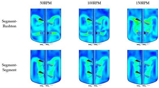
In this study, CFD simulations were applied to comprehensively investigate the influence of impeller configuration and RPM on the mixing performance and hydrodynamic behaviour of a laboratory-scale bioreactor operating in the turbulent regime. Two different impeller configurations (Segment–Segment and Segment–Rushton) and three different RPM values (50, 100, and 150) were used in the CFD simulations. To validate the CFD model, the power values obtained from the CFD models were compared with the experimentally measured power values. The power values were in close agreement. This indicated that the CFD models could represent the experimentations accurately. For simulations with the Segment–Rushton impeller configuration, it was observed that, at the lowest RPM value (50), two impellers operated independently with minimum interaction. The Rushton and Segment impellers discharged the flow in radial and axial directions, respectively. However, as RPM was increased, the intensity of the interaction between the impellers increased. At the highest RPM value, the high axial flow generated by the Segment impeller altered the fluid hydrodynamics around the Rushton impeller considerably and the Rushton impeller did not operate as a radial impeller. For simulations with the Segment–Segment impeller configuration, two impellers interacted and two circulation loops were created in the fermenter tank in all cases. CFD simulations demonstrate that, at a constant RPM, the Segment–Rushton impeller configuration had higher P t o t a l and N p , t o t a l values, average strain rate magnitude, average τ t values, and lower F l t o t a l values compared to the Segment–Segment impeller configuration. It then could be concluded that the Segment–Rushton impeller configuration may not be suitable for cultivation of shear-sensitive microorganisms. Calculating the mixing time and energy consumption showed that, at low RPM values (50 and 100), the Segment–Segment impeller configuration had a better performance. However, at the highest RPM, the Segment–Rushton impeller had a shorter mixing time and energy consumption, which could be attributed to the high turbulent flow generated by this type of impeller configuration. The CFD simulation results also showed that increasing the RPM increased the P t o t a l values, average strain rate magnitude, and average τ t values and shortened the mixing time regardless of the impeller configuration employed.
This study shows that CFD can be used as a valuable tool to obtain detailed information regarding the stirred bioreactors which might otherwise be challenging or impossible to obtain experimentally. With the rapid advancement in computational facilities, more accurate but computationally demanding simulation techniques such as LES and DNS can be used in future studies to simulate stirred bioreactors. These approaches can provide a more comprehensive understanding of the system.

Author Contributions

Conceptualization, M.E., M.T., and F.E.-M.; methodology, M.E., M.T., and F.E.-M.; software, M.E.; validation, M.E., R.M.V., and A.C.; formal analysis, M.E., M.T., R.M.V., A.C., and F.E.-M.; resources, F.E.-M., M.T., R.M.V., and A.C.; writing—original draft preparation, M.E.; writing—review and editing, F.E.-M. and M.T.; supervision, F.E.-M. and M.T.; funding acquisition, F.E.-M. and M.T.

Funding

The financial support provided through the Mitacs accelerate program is gratefully acknowledged.

Conflicts of Interest

The authors declare no conflict of interest.

Nomenclature

C (m)Clearance N p (-)Power number
D (s−1)Strain rate P (W)Power
D i (m)Impeller diameter S c t ( -)Turbulent Schmidt number
D R (m)Rushton impeller diameterT (m)Tank internal diameter
D S (m)Segment impeller diameter U (m/s)Fluid velocity
D i , m (m2/s) Mass-diffusion coefficient U r (m/s)Radial velocity
d c e l l (m)Cell diameter U z (m/s)Axial velocity
F l r (-)Radial flow number Y i (-)Mass fraction of species i
F l z (-)Axial flow number ε (W/kg)Turbulence dissipation rate
H (m)Spacing between impellers ρ (kg/m3)Fluid density
J i   (kg/m2 s)Diffusion flux of species i μ (Pa s)Dynamic viscosity
L H (m)Liquid height μ t (Pa s)Turbulent viscosity
l e (m)Kolmogorov length scale ν (m2/s)Kinematic viscosity
M (N m)Torque τ t ,   τ d (Pa)Stress acting on cell due to turbulence
N (s−1)Impeller speed θ m (s)Mixing time

References

  1. Amanullah, A.; Buckland, B.C.; Nienow, A.W. Mixing in the Fermentation and Cell Culture Industries. In Handbook of Industrial Mixing; John Wiley & Sons: Hoboken, NJ, USA, 2004; pp. 1071–1170. [Google Scholar]
  2. Zhou, T.; Zhou, W.; Hu, W.; Zhong, J. Bioreactors, cell culture, commercial production. Encycl. Ind. Biotechnol. Bioprocess Biosep. Cell Technol. 2009, 1–18. [Google Scholar] [CrossRef]
  3. Patwardhan, A.W.; Joshi, J.B. Relation between Flow Pattern and Blending in Stirred Tanks. Ind. Eng. Chem. Res. 1999, 38, 3131–3143. [Google Scholar] [CrossRef]
  4. Bustamante, M.; Cerri, M.; Badino, A.C. Comparison between average shear rates in conventional bioreactor with Rushton and Elephant ear impellers. Chem. Eng. Sci. 2013, 90, 92–100. [Google Scholar] [CrossRef]
  5. Jüsten, P.; Paul, G.C.; Nienow, A.W.; Thomas, C.R. Dependence of mycelial morphology on impeller type and agitation intensity. Biotechnol. Bioeng. 1996, 52, 672–684. [Google Scholar] [CrossRef]
  6. Vrábel, P.; Van Der Lans, R.G.; Luyben, K.C.; Boon, L.; Nienow, A.W. Mixing in large-scale vessels stirred with multiple radial or radial and axial up-pumping impellers: Modelling and measurements. Chem. Eng. Sci. 2000, 55, 5881–5896. [Google Scholar] [CrossRef]
  7. Zhu, H.; Nienow, A.W.; Bujalski, W.; Simmons, M.J. Mixing studies in a model aerated bioreactor equipped with an up- or a down-pumping ‘Elephant Ear’ agitator: Power, hold-up and aerated flow field measurements. Chem. Eng. Res. Des. 2009, 87, 307–317. [Google Scholar] [CrossRef]
  8. Collignon, M.-L.; Delafosse, A.; Crine, M.; Toye, D. Axial impeller selection for anchorage dependent animal cell culture in stirred bioreactors: Methodology based on the impeller comparison at just-suspended speed of rotation. Chem. Eng. Sci. 2010, 65, 5929–5941. [Google Scholar] [CrossRef] [Green Version]
  9. Venkat, R.V.; Chalmers, J.J. Characterization of agitation environments in 250 mL spinner vessel, 3 L, and 20 L reactor vessels used for animal cell microcarrier culture. Cytotechnology 1996, 22, 95–102. [Google Scholar] [CrossRef]
  10. Simmons, M.; Zhu, H.; Bujalski, W.; Hewitt, C.; Nienow, A. Mixing in a Model Bioreactor Using Agitators with a High Solidity Ratio and Deep Blades. Chem. Eng. Res. Des. 2007, 85, 551–559. [Google Scholar] [CrossRef]
  11. Rutherford, K.; Lee, K.C.; Mahmoudi, S.M.S.; Yianneskis, M. Hydrodynamic characteristics of dual Rushton impeller stirred vessels. AIChE J. 1996, 42, 332–346. [Google Scholar] [CrossRef]
  12. Kazemzadeh, A.; Ein-Mozaffari, F.; Lohi, A.; Pakzad, L. Effect of Impeller Spacing on the Flow Field of Yield-Pseudoplastic Fluids Generated by a Coaxial Mixing System Composed of Two Central Impellers and an Anchor. Chem. Eng. Commun. 2017, 204, 453–466. [Google Scholar] [CrossRef]
  13. Hari-Prajitno, D.; Mishra, V.P.; Takenaka, K.; Bujalski, W.; Nienow, A.W.; Mckemmie, J. Gas-liquid mixing studies with multiple up- and down-pumping hydrofoil impellers: Power characteristics and mixing time. Can. J. Chem. Eng. 1998, 76, 1056–1068. [Google Scholar] [CrossRef]
  14. Kazemzadeh, A.; Ein-Mozaffari, F.; Lohi, A.; Pakzad, L. Investigation of hydrodynamic performances of coaxial mixers in agitation of yield-pseudoplasitc fluids: Single and double central impellers in combination with the anchor. Chem. Eng. J. 2016, 294, 417–430. [Google Scholar] [CrossRef]
  15. Odeleye, A.; Marsh, D.; Osborne, M.; Lye, G.; Micheletti, M. On the fluid dynamics of a laboratory scale single-use stirred bioreactor. Chem. Eng. Sci. 2014, 111, 299–312. [Google Scholar] [CrossRef] [PubMed] [Green Version]
  16. Werner, S.; Kaiser, S.C.; Kraume, M.; Eibl, D. Computational fluid dynamics as a modern tool for engineering characterization of bioreactors. Pharm. Bioprocess. 2014, 2, 85–99. [Google Scholar] [CrossRef]
  17. Kelly, W.J. Using computational fluid dynamics to characterize and improve bioreactor performance. Biotechnol. Appl. Biochem. 2008, 49, 225. [Google Scholar] [CrossRef] [PubMed]
  18. Delafosse, A.; Liné, A.; Morchain, J.; Guiraud, P. LES and URANS simulations of hydrodynamics in mixing tank: Comparison to PIV experiments. Chem. Eng. Res. Des. 2008, 86, 1322–1330. [Google Scholar] [CrossRef]
  19. Haringa, C.; Mudde, R.F.; Noorman, H.J. From industrial fermentor to CFD-guided downscaling: What have we learned? Biochem. Eng. J. 2018, 140, 57–71. [Google Scholar] [CrossRef]
  20. Kaiser, S.C.; Löffelholz, C.; Werner, S.; Eibl, D. CFD for Characterizing Standard and Single-Use Stirred Cell Culture Bioreactors. In Computational Fluid Dynamics Technologies and Applications; IntechOpen: London, UK, 2011. [Google Scholar]
  21. Hashemi, N.; Ein-Mozaffari, F.; Upreti, S.R.; Hwang, D.K. Hydrodynamic characteristics of an aerated coaxial mixing vessel equipped with a pitched blade turbine and an anchor. J. Chem. Technol. Biotechnol. 2018, 93, 392–405. [Google Scholar] [CrossRef]
  22. Azargoshasb, H.; Mousavi, S.M.; Jamialahmadi, O.; Shojaosadati, S.A.; Mousavi, S.B. Experiments and a three-phase computational fluid dynamics (CFD) simulation coupled with population balance equations of a stirred tank bioreactor for high cell density cultivation. Can. J. Chem. Eng. 2016, 94, 20–32. [Google Scholar] [CrossRef]
  23. Panneerselvam, R.; Savithri, S.; Surender, G.D. CFD modeling of gas–liquid–solid mechanically agitated contactor. Chem. Eng. Res. Des. 2008, 86, 1331–1344. [Google Scholar] [CrossRef]
  24. Liu, Y.; Wang, Z.-J.; Xia, J.-Y.; Haringa, C.; Liu, Y.-P.; Chu, J.; Zhuang, Y.-P.; Zhang, S.-L. Application of Euler Lagrange CFD for quantitative evaluating the effect of shear force on Carthamus tinctorius L. cell in a stirred tank bioreactor. Biochem. Eng. J. 2016, 114, 209–217. [Google Scholar] [CrossRef]
  25. Singh, H.; Fletcher, D.F.; Nijdam, J.J. An assessment of different turbulence models for predicting flow in a baffled tank stirred with a Rushton turbine. Chem. Eng. Sci. 2011, 66, 5976–5988. [Google Scholar] [CrossRef]
  26. Aubin, J.; Fletcher, D.F.; Xuereb, C. Modeling turbulent flow in stirred tanks with CFD: The influence of the modeling approach, turbulence model and numerical scheme. Exp. Therm. Fluid Sci. 2004, 28, 431–445. [Google Scholar] [CrossRef]
  27. Nienow, A.W. Reactor Engineering in Large Scale Animal Cell Culture. Cytotechnology 2006, 50, 9–33. [Google Scholar] [CrossRef] [Green Version]
  28. Sorg, R.; Tanzeglock, T.; Périlleux, A.; Solacroup, T.; Broly, H.; Soos, M.; Morbidelli, M. Minimizing hydrodynamic stress in mammalian cell culture through the lobed Taylor-Couette bioreactor. Biotechnol. J. 2011, 6, 1504–1515. [Google Scholar] [CrossRef]
  29. Tanzeglock, T.; Šoóš, M.; Stephanopoulos, G.; Morbidelli, M. Induction of mammalian cell death by simple shear and extensional flows. Biotechnol. Bioeng. 2009, 104, 360–370. [Google Scholar] [CrossRef]
  30. Fluent, 12.0 Theory Guide; Ansys Inc.: Canonsburg, PA, USA, 2009.
Figure 1. The fermenter geometries (front view) (a) with the Segment–Rushton impeller and (b) with the Segment–Segment impeller: the baffles were removed for clarity; (c,d) the fermenter geometries including baffles.
Processes 07 00694 g001
Figure 2. Comparison of instantaneous velocity magnitudes for simulations with different mesh sizes (at 15 s of simulation).
Processes 07 00694 g002
Figure 3. Velocity contour and velocity vector Case 1 (a,b), Case 2 (c,d), and Case 3 (e,f).
Processes 07 00694 g003
Figure 4. Velocity contour and velocity vector Case 4 (a,b), Case 5(c,d), and Case 6 (e,f).
Processes 07 00694 g004
Figure 5. Effect of RPM on axial velocity profiles (a) with Segment–Rushton impeller configuration and (b) with Segment–Segment impeller configuration (SR and SS stand for Segment–Rushton and Segment–Segment impeller configurations, respectively): The following numbers show the applied RPM).
Processes 07 00694 g005
Figure 6. Effect of impeller configuration on axial velocity profiles: (a) 50 RPM, (b) 100 RPM, and (c) 150 RPM (SR and SS stand for Segment–Rushton and Segment–Segment impeller configurations, respectively).
Processes 07 00694 g006
Figure 7. τ t contours: (a) Case 1, (b) Case 2, (c) Case 3, (d) Case 4, (e) Case 5, and (f) Case 6.
Processes 07 00694 g007
Figure 8. Location of monitoring points for the mixing-time calculation.
Processes 07 00694 g008
Figure 9. Tracer response curve for different points (Case 5 simulation).
Processes 07 00694 g009
Table 1. Dimensions of fermenter vessel and impellers.
ParameterValue
T (m)0.263
C (m)0.088 (T/3)
DR (m)0.103 (~T/3)
DS (m)0.132 (T/2)
H (m)¾ DS
LH (m)1.14T
Shaft size (m)0.018
Baffle width (m)0.025 (~T/10)
Segment blade angle relative to the horizontal 30°
Table 2. Experimental cases.
RPMImpeller Configuration
Case 150Segment–Rushton
Case 2100
Case 3150
Case 450 Segment–Segment
Case 5100
Case 6150
Table 3. R e values for different simulation cases.
Case 1Case 2Case 3Case 4Case 5Case 6
R e ( ) × 10 4 1.172.343.501.452.904.3
Table 4. Computational fluid dynamics (CFD) simulation settings.
CFD Parameters
Fluid density (kg/m3)1000
Fluid viscosity (Pa s)0.001
Spatial discretization schemeQUICK
Pressure–velocity couplingSIMPLEC
Transient formulation Second Order Implicit
Time step (s)0.001
Table 5. Comparison between the experimental and CFD results.
Power   ( W )
ExperimentCFDError (%)
Case 10.04360.0380 13.1
Case 20.279 0.306 9.46
Case 31.311.1413.3
Case 40.02620.023410.5
Case 50.1570.1665.54
Table 6. Power and power numbers obtained from CFD results for different cases.
P   ( W ) N p P t o t a l   ( W ) N p , t o t a l
Case 1Segment0.01580.6800.03803.98
Rushton0.02223.30
Case 2Segment0.1320.7120.3063.94
Rushton0.1743.23
Case 3Segment0.5270.8411.144.20
Rushton0.6093.36
Case 4Upper-Segment0.01610.6960.02341.01
Lower-Segment0.007290.315
Case 5Upper-Segment0.1200.6480.1660.894
Lower-Segment0.04560.246
Case 6Upper-Segment0.4090.6530.5470.873
Lower-Segment0.1380.220
Table 7. Values of strain rate magnitude for different simulation cases.
D   ( 1 / s )
Case 1Rushton zone18.1
Segment zone10.9
Rest of the tank 6.10
Average values11.7
Case 2Rushton zone39.8
Segment zone21.0
Rest of the tank13.0
Average values24.6
Case 3Rushton zone70.0
Segment zone36.2
Rest of the tank18.2
Average values41.5
Case 4Upper-Segment zone10.5
Lower-Segment zone9.00
Rest of the tank 5.10
Average values8.20
Case 5Upper-Segment zone19.8
Lower-Segment zone15.8
Rest of the tank 9.50
Average values15.03
Case 6Upper-Segment zone29.2
Lower-Segment zone23.1
Rest of the tank 14.6
Average values22.3
Table 8. Values of ε a v g , l e , and τ t for different simulation cases.
ε a v g   ( W / k g ) × 10 4 l e   ( m ) × 10 5 τ t   ( P a ) × 10 2
Case 1Rushton zone46.612.16.83
Segment zone19.715.04.44
Rest of the tank 9.7017.93.11
Average values25.315.04.79
Case 2Rushton zone3377.3818.3
Segment zone1249.4811.1
Rest of the tank73.710.88.58
Average values1789.2212.7
Case 3Rushton zone14605.1138.2
Segment zone6066.3724.6
Rest of the tank1958.4714.0
Average values7546.6525.6
Case 4Upper-Segment zone17.915.44.23
Lower-Segment zone13.116.63.62
Rest of the tank 5.3820.82.32
Average values12.117.63.39
Case 5Upper-Segment zone1039.9210.2
Lower-Segment zone72.410.88.51
Rest of the tank 34.513.05.87
Average values70.011.38.18
Case 6Upper-Segment zone2947.6417.1
Lower-Segment zone2128.2814.6
Rest of the tank 1109.7710.5
Average values2058.5614.1
Table 9. Flow numbers for different simulation cases.
F l r F l z F l s = F l r + F l z
(for Each Impeller)
F l t o t a l
Case 1Rushton 0.4080.2910.699 1.05
Segment 0.08090.2730.354
Case 2Rushton 0.4250.264 0.689 0.964
Segment 0.02990.2450.275
Case 3Rushton 0.00668 0.4080.4150.835
Segment 0.3670.05160.419
Case 4Upper-Segment 0.3670.1330.5011.32
Lower-Segment 0.2310.5860.817
Case 5Upper-Segment 0.3390.1660.5061.33
Lower-Segment 0.2360.5480.820
Case 6Upper-Segment 0.353 0.1500.5031.32
Lower-Segment 0.2250.5890.813
Table 10. Mixing time values for different simulation cases.
Case 1Case 2Case 3Case 4Case 5Case 6
θ m ( s ) 61.437.27.8134.321.517.2
Table 11. Energy consumption values for different simulation cases.
Case 1Case 2Case 3Case 4Case 5Case 6
P t o t a l × θ m   ( J ) 2.3311.48.870.7883.569.39

