Numerical Analysis of the Diaphragm Valve Throttling Characteristics

Abstract

The throttling characteristics of the diaphragm valve are numerically studied in this paper. Firstly, the diaphragm deformation performance is analyzed by a finite element method, while the upper boundary morphology of the internal flow field under different valve openings was obtained. Then the two-dimensional simulation of the weir diaphragm valve flow field is carried out in order to explore the optimal design of flow path profile. The study shows that the throttling characteristics can be improved by flatting the ridge side wall, widening the top of the ridge and gently flatting the internal protruding of the flow path. In addition, using the local grid encryption techniques based on velocity gradient adaptive and y⁺ adaptive can improve the accuracy of simulation results. Finally, a cavitation two-phase flow simulation is carried out. The results show that cavitation may occur below 50% opening of diaphragm valve in ultra-pure water system, which becomes more intense with the increase of inlet pressure and even leading to flow saturation on the micro-orifice state.

1. Introduction

The diaphragm valves are extensively used in various industrial applications, including breweries, pharmaceutical chemical, dairy, food, petroleum and mining etc. [1]. This is due to several unique advantages: the ability to handle solids, the low resistance coefficient, no dead areas where particles may collect, easy maintenance, and automation [1,2,3]. Traditionally, the diaphragm valves are commonly used as shut-off valves for non-Newtonian fluids with variable viscosities [4], such as suspensions, mixed solutions, and the like, because diaphragm valves in such applications do not need and are not easy to achieve accurate flow control. With the rapid development of information technology, diaphragm valves have been widely used in the precise control of Newtonian fluids with downsizing technology trend [5,6]. In order to obtain higher integration and smaller feature sizes of the chip, immersion lithography is the cutting-edge technology and key step in the semiconductor industry [7,8]. The fluid control requirements for ultra-pure water treatment and liquid injection systems are becoming more stringent, which mainly reflects the water purity of ultra-pure water and the stability of immersion flow field [9,10]. Diaphragm valves are the key components of ultra-pure water systems due to their excellent cleanliness and low resistance loss, ensuring a stable flow balance of the infusion flow and the immersion flow field [11].

The diaphragm valve structure and diaphragm material affect the throttling characteristics and sealing performance [12]. From the structural point of view, the most widely used diaphragm valves are straight-through type and weir type [1,13]. Although the flowing resistance in straight-through type valve body is lower and the flow performance is better than that in weir type valve body, the diaphragm travels longer in straight-through type, which means that under the condition of frequent opening and closing control, the life of the straight-through type valve body diaphragm will be much lower than that of the weir type valve body diaphragm. In addition, during the closing process in weir type valve body, the diaphragm forms a vertical coincident seal with the sealing table without any mechanical friction, thereby meeting the sanitary level cleaning requirements. Based on the special advantages of the weir type, the diaphragm valves used in the semiconductor industry are mostly weir type valve bodies. From the material point of view, the properties of rubber diaphragm such as high temperature resistance and oil resistance in the field of chemical industry are not the key points to be considered in ultra-pure water system. The surface quality, tensile strength, fatigue strength and shape retention of rubber are more suitable for evaluating diaphragm valve diaphragm in ultra-pure water system. Currently NBR, HNBR, ACM, FKM, etc. are the most widely used rubber material [14]. Nickel or silicon or bimorph materials are also used as diaphragm materials [15,16]. In addition, The diaphragm made of fluoroplastics (PTFE as an example) or rubber and fluoroplastics composite materials has better elasticity and strength, and its surface is smoother [17].

The throttling characteristics and flow control performance of the diaphragm valve are expressed in the form of valve flow coefficient C_v (or K_v) value, local resistance coefficient and valve flow characteristic curve [18,19]. The valve flow coefficient K_v value is the unit of measurement in metric units (the valve flow coefficient in English units is called the C_v value) and is defined as: under the standard pressure drop of 1 bar, the volume flow rate of water (the fluid severity at 1 N/m³) through the valve per hour, as expressed in Equation (1).

$$K_v=Q\sqrt{\frac{{\rho }_0}{\Delta p}}$$

(1)

where, K_v—valve flow coefficient; Q—volume flow rate (m³/h); Δp—pressure drop (1 bar); ρ₀—density of water (kg/m³).

The resistance coefficient is the index to measure the pressure loss of the valve. It is a dimensionless coefficient representing the pressure loss of the valve. It depends on the type, diameter, structure and cavity shape of the valve, and is calculated by the experimental data of the valve. According to the Bernoulli equation, the formula for calculating the drag coefficient can be deduced as Equation (2) [20],

$$\zeta =\frac{2\Delta p}{\rho v^2}$$

(2)

where, ρ—density of medium (kg/m³); v—average velocity of inlet (outlet) (m/s); Δp—pressure drop (Pa).

The flow characteristic curve of the valve shows the flow through the valve at different openings in the process of opening and closing [21]. It is an index to describe the flow control performance of the valve. The higher the linearity of the curve, the larger the linearity range, the better the flow control performance of the valve. The curve was obtained experimentally.

At present, there are many experimental studies and valve body structure improvement studies on diaphragm valves, mainly focusing on sealing performance and operability. There are also studies on throttling characteristics of diaphragm valves and simulation studies on flow field [6,22,23] and pressure characteristics [24,25], but not in the ultra-pure water system of the semiconductor industry. Various studies based on other types of valves have confirmed that the change of flow path shape and the use of pilot valves can improve flow control characteristics, reduce vibration and cavitation [26,27,28,29]. The weir type diaphragm valve has become the mainstream for the sake of better cleanliness, longer diaphragm life, and better flow control characteristics. However, due to its large flow resistance and lack of design criteria for internal flow channel surface structure, it is difficult to obtain optimization methods to further improve valve control performance. In addition, the outlet of diaphragm valves in ultra-pure water treatment system is generally atmospheric back pressure environment, but the pressure in the pipeline of ultra-pure water treatment system is generally about 5 times atmospheric pressure, so it is easy to produce cavitation and jet under the condition of diaphragm valve micro-orifice, leading to flow saturation and further increase pressure loss.

In order to solve the above problems, based on the structure of the weir type diaphragm valve body, the numerical simulation analysis of two-dimensional flow field is carried out. By comparing the flow coefficient, resistance coefficient and flow characteristic curve, the flow control performance of valves with different profiles is evaluated, and the structural optimization scheme is proposed and verified. Using the local grid encryption techniques based on velocity gradient adaptive and y⁺ adaptive the accuracy of simulation results are improved [30]. The flow field of diaphragm valve was simulated and analyzed, and the cavitation phenomenon of small valve opening of diaphragm valve was explored under the condition of ultra-pure water system.

2. Finite Element Analysis of Diaphragm Deformation

The flow path surface structure of weir type diaphragm valve is determined not only by the shape of the bottom ridge and the tube wall itself, but also by the deformation of the diaphragm bottom surface and the angle of the installation joint at different openings. A number of shape elements determine the upper and lower wall boundary of the two-dimensional flow field of weir type diaphragm valve.

However, the rubber diaphragm is hyper elastic and irregular in shape. It is difficult to calculate the deformation by theoretical calculation [31,32]. At present, there are few experimental or simulation results for the diaphragm deformation when the diaphragm valve works. Therefore, in order to obtain the inner surface shape of the diaphragm at different openings and determine the changing two-dimensional flow field boundary, firstly, finite element method analysis on the diaphragm of diaphragm valve is carried out.

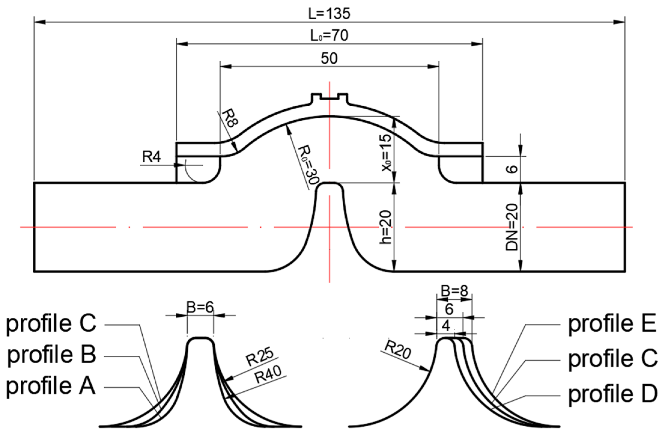
2.1. Structure and Grid

According to the design method of diaphragm size of diaphragm valve, based on the nominal size DN20 series of diaphragm valve, the shape and size of diaphragm are preliminarily determined (Figure 1). The effects of the diaphragm thickness (B₀ = 4 mm, B₀ = 5 mm, B₀ = 6 mm) and the stem loading surface diameter on the diaphragm deformation were investigated.

The three-dimensional model of rubber diaphragm is imported into ANSYS static structure and meshed into model interface. Based on the mesh automatic meshing basic set value, the size function is selected adapted, and the relevance center selects course, and the mesh size is 1 mm. The hyper elastic material was selected as the model material. The neoprene rubber was extracted from ANSYS engineering data, and the density (ρ₁ = 1.25 g/cm³) and tensile strength (σ > 10 MPa) of the material were manually added. Figure 2a shows the model mesh with a diaphragm thickness of B₀ = 6 mm. The results show that the maximum skewness is 0.81, 0.81 and 0.82 under the three thicknesses, and the average is less than 0.5. The grid quality is good.

Load setting (

Table A1. Simulation settings and parameters.

The FEM Simulation of the Diaphragm
Grid size	1 mm	Engineering data sources	Neoprene rubber
Density	1.25 g/cm3	Tensile ultimate strength	100 MPa
Design modeller	Add extrude	Mesh	Size function:adaptive
Relative center	Coarse	Static structure	Structural
Analysis settings	Program controlled	Large deflection	On
Standard earth gravity	All bodies	Fixed support	Upper and lower ring extruded surfaces
Fixed displacement	1.5–15 mm	Frictionless support	Loading stage inner wall
Solution	Total deformation	Solution	Equivalent stress
The Two-Dimension Simulation of the Weir-Type Diaphragm Valve Flow Filed
Basic grid size	1 mm	General: type	Pressure-based
General: time	Steady	Velocity formulation	Absolute
Viscous model	Standard k-epsilon	Near-wall treatment	Standard wall functions
Model constants	Default	Materials	Fluid:water-liquid
Velocity inlet	0.5–0.8 m/s	Initial gauge pressure	400 kPa
Turbulence parameters	Based on calculation	Pressure outlet	Total pressure
Wall roughness constant	0.02	Solution methods	Simple
Pressure	Standard	Momentum	Second order upwind
Turbulent kinetic energy	Second order upwind	Solution controls	Default
Iterations	50,000	Monitor check absolute criteria	0.001
The cavitation simulation of small valve orifice state
Grid size	1 mm	General: type	Pressure-based
General: time	Steady	Velocity formulation	Absolute
Multiphase model	Mixture	Phase interaction	Mass: mechanism
Cavitation model	Zwart-Gerber-Belamri	Cavitation properties	Constant 3540
Model constants	Default	Phase 1	Water-liquid
Phase 2	Water-vapor	Viscous model	Realizable k-epsilon
Near wall treatment	Standard wall functions	Pressure inlet	500–1600 kPa
Turbulent intensity	5%	Hydraulic diameter	0.02
Pressure outlet	100 kPa	Outlet backflow pressure	Total pressure
Inlet volume fraction	Phase 2: 0 (constant)	Solution methods	Scheme: simple
Spatial discretization	Pressure: PRESTO!	Other settings	Second order upwind
Solution controls	All (0.1–0.2)	Number of interactions	50,000

): Select large deformation in analysis setting, apply fixed load (flange of diaphragm upper and lower surface, simulate assembly fixing), standard gravity, uniform pressure (arc under diaphragm, simulate medium back pressure), fixed displacement (stem action plane, direction downward, x₀ = 15 mm, solve maximum deformation), and add no friction load (loading the side wall, limiting the deformation of the cylindrical surface). The resolver outputs the total displacement map, the longitudinal section displacement map and the longitudinal section stress map. Figure 2b shows the total deformation of the diaphragm with a thickness of B₀ = 4 mm.

2.2. Analysis and Conclusion

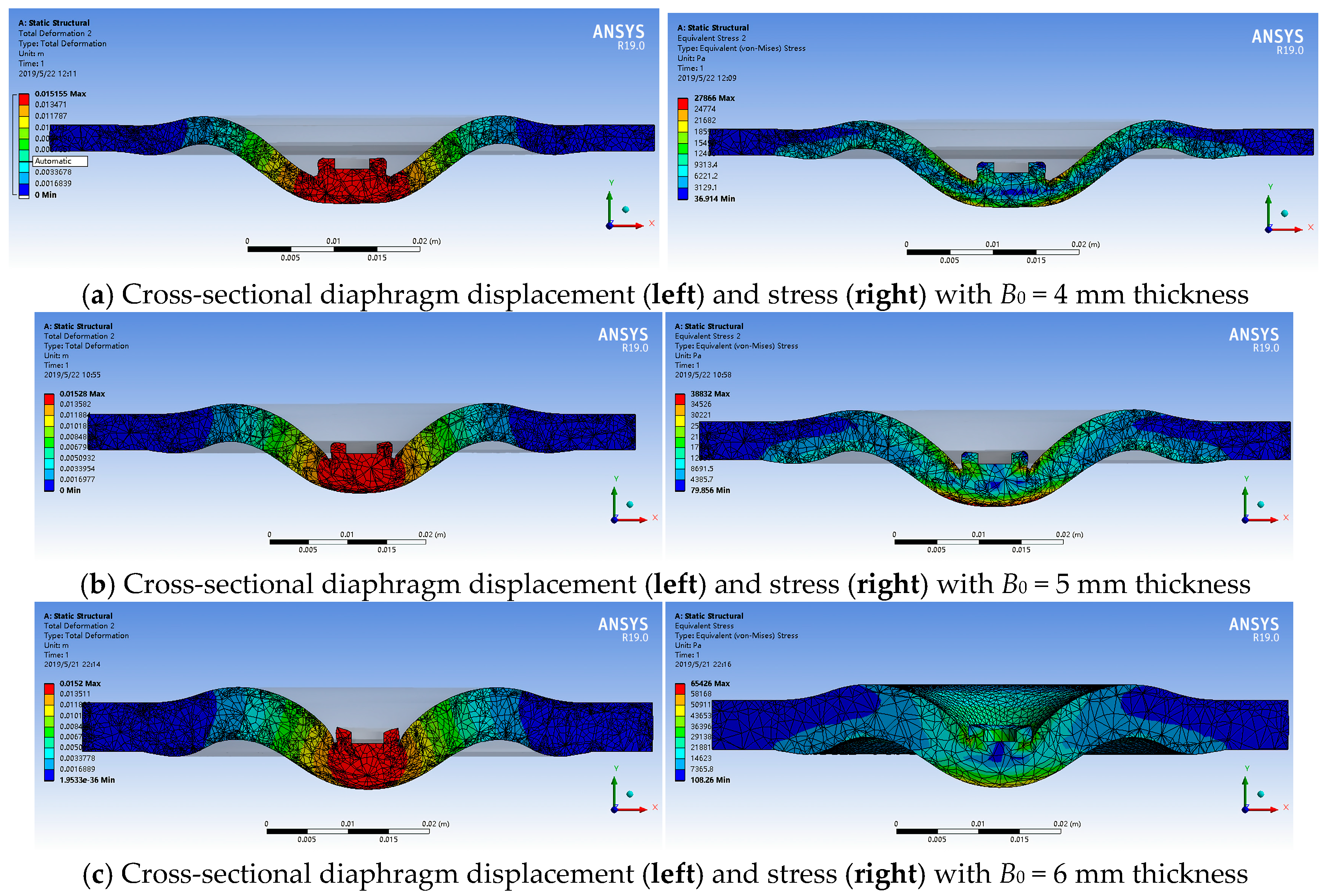
2.2.1. The Influence of Diaphragm Thickness

Contrastive displacement diagram (Figure 3) shows that with the decrease of diaphragm thickness, the maximum strain region increases gradually, the strain distribution is more uniform and the strain transmission is better. That is, the displacement input of valve stem can be well maintained to the surface of diaphragm, so that the diaphragm can produce a certain amount of deformation with the input requirements, and the runner can produce the corresponding opening. From this point of view, the thinner diaphragm is more conducive to the diaphragm valve flow accurate control. In addition, the thinner the diaphragm, the smoother the deformation at the bottom, the approximate planes at the maximum displacement, the larger the contact area with the top of the ridge, and the better the sealing performance.

However, this does not mean that the thinner the diaphragm, the better. Contrast stress diagram (Figure 3) shows that the thinner the diaphragm valve is, the greater the maximum stress is, and the greater the maximum stress area is, especially the upper and lower surface of the diaphragm. The thicker the diaphragm, the lower the stress is in most areas. The maximum stress is only concentrated in the sealing contact area of the diaphragm bottom surface, and sticks to the ridge top. After tightening, part of the stress is offset, which means that the possibility of diaphragm damage is reduced and the life of the diaphragm is longer.

2.2.2. Effect of Stem Loading Area

By analyzing the deformation of diaphragm (Figure 4) under different loading areas, it can be seen that when the valve stem is loaded in a large area, there is almost no stress at the center of the diaphragm and the maximum displacement is not reached. On the contrary, the maximum displacement occurs directly below the edge of the convex platform. When the maximum displacement of the valve stem is input, the center of the diaphragm bottom surface is depressed. It shows that the displacement input cannot be transmitted well. Moreover, due to the concave surface under the diaphragm, the diameters above the ridge have undergone two shrinkage and expansion processes. The continuous change of the diameters will also lead to increased pressure loss and increase the resistance coefficient of the valve. In addition, this kind of depression will also lead to incomplete sealing and easy to leak.

When the diaphragm is loaded in a moderate area, the central area of the lower surface is close to the plane, the boundary of the runner is more uniform, and the sealing performance is better. The diaphragm deflection cannot meet the working requirement when the minimum area load or approximately concentrated load occurs. Even some element grids have been seriously damaged during the simulation iteration process, which leads to the termination of the simulation, indicating that the loading area of the valve stem should not be too small.

By exploring the deformation of diaphragm at different opening, using FEM module in ANSYS WORKBENCH, the geometric model of the deformed diaphragm is obtained, and the shape and size of the diaphragm under different opening are obtained. The flow field boundary at different opening can be obtained by matching the shape of the runner.

3. CFD Flow Structure and Grid Independence Analysis

3.1. Two-Dimensional Flow Field Model of Weir Diaphragm Valve

The diaphragm of Weir-Type diaphragm valve is deformed and displaced by the stem loading, and the diameter of flow passage is compressed to achieve throttling effect until it is fitted with the sealing table at the top of the ridge to realize the complete closure of the valve (Figure 5).

In this paper, the LiquidlensTMLLG4 ultra-pure water treatment system of ENTEGRIS Company is taken as the reference of working condition of diaphragm valve. The relevant size parameters of DS12-2M-12F-3 manual diaphragm valve are taken as the reference for modeling. The flow field structure size can be obtained by simplification (Figure 6). The shape of the ridge has a major influence on the flow state and loss of the medium in the weir diaphragm valve. Five different sizes of the ridge structures (Figure 6) are designed to explore their effects on the flow characteristics of the diaphragm valve.

Determine the relevant flow parameters according to the reference operating conditions (

Table 1. Liquidlens^TMLLG4 System Flow Parameter Index.

	Parameters	Units	Index
System inlet index	Flow rate range	L/min	>8
	Pressure range	kPa	350~550
	Temperature rage	°C	17~26
System outlet index	Flow rate range	L/min	1~8
	Pressure range	kPa	100~500
	Temperature rage	°C	17~24

).

The diaphragm valve is used at the inlet and outlet of the system, so the back pressure at the outlet of the simulated diaphragm valve is generally set to p_out = 400 kPa. When the nominal diameter of diaphragm valve is DN = 20 mm and the system flow rate Q is set to 8 L/min, the average velocity of flow can be calculated from Equation (3),

$$v=\frac{Q}{A}=\frac{4Q}{\pi {(DN)}^2}$$

(3)

The average velocity of flow can be calculated to be about v = 0.42 m/s. According to the table above, the flow rate varies in the vicinity of 8 L/min. Therefore, a set of different flow velocities is set up in simulation to explore the characteristics of diaphragm valves under different Reynolds numbers.

In addition, according to the deformation results of diaphragm at different openings, the two-dimensional flow field model of valve at different openings can be obtained (profile E as an example in Figure 7).

3.2. Boundary Conditions and Simulation Settings

After the flow field model is established, the mesh module is used to mesh the flow field and discrete flow fields. Select the adaptation in the size function, select the course in the relevant center, and set the grid size to 1 mm, 0.5 mm, and 2 mm respectively to generate the mesh. The meshing results are as shown in Figure 8 for the profile E. The simulation parameters in detail are shown in Table A1.

The skewness is checked in the grid quality column, and the maximum skewness of the three meshes is 0.593 (1 mm), 0.539 (0.5 mm) and 0.504 (2 mm), respectively. All of these can meet the requirements of this simulation. In order to reduce the computational complexity of the simulation iteration and ensure a certain degree of accuracy, this simulation is other. The grid size of each basin shape is set to 1 mm.

The grid file is imported into FLUENT software, and the environment is two-dimensional flow field simulation. The acceleration of gravity is added in general. Model models select standard k-ε model, and model parameters follow the default values of the system. Water-liquid is added to the liquid medium material, and the default parameters are obtained. The wall material is made of steel as the prototype. Some parameters are modified, such as the absolute roughness value is changed to Δ = 0.02. The other parameters can be maintained by default because heat exchange is not involved in this time.

Boundary conditions: The inlet is the velocity inlet. When the relationship between Reynolds number and valve flow coefficient is simulated, the velocity input range is from v = 0.3 m/s to v = 0.8 m/s, and the interval is 0.05 m/s. When investigating the influence of ridge shape, the input is v = 0.5 m/s; the outlet is a pressure outlet, and the back pressure is p_out = 400 kPa; the characteristic parameters such as turbulent intensity, hydraulic diameter (DN = 0.02 m), turbulent energy k, turbulent dissipation rate ε, turbulent viscosity ratio in the setting of inlet and outlet can be calculated according to the following formulas.

$$i=0.16{\mathrm{Re}}^{(-1/8)}$$

(4)

$$k=1.5{(vi)}^2$$

(5)

$$\epsilon =0.75C_{\mu }{k}^{1.5}/l=0.75C_{\mu }{k}^{1.5}/(0.07d)$$

(6)

$${\mu }_t={\rho }_0{C}_{\mu }\frac{k^2}{\epsilon }$$

(7)

Among them, C_μ = 0.09, v is the velocity of flow, ρ₀ is the density of water, μ_t/μ is the turbulent viscosity ratio, and μ is the dynamic viscosity of water.

Solver method sets pressure as standard, calculates second-order upwind, and sets reference cross-section at the center of the valve orifice, so as to output characteristic parameters at the valve orifice in the calculation results. The simulation step size is set to 5000 steps, and other parameters such as relaxation factor and convergence residual range are all defaulted by the system.

The surface integrals are selected from the simulation results to output the results. By calculating the total pressure at the inlet, outlet and the middle section of the valve, the pressure loss between the outlet and the inlet can be obtained, and the flow coefficient C_v (K_v) and local resistance coefficient ζ can be calculated according to Equations (1) and (2).

3.3. Mesh Refinement and Grid Independence Verification Based on Velocity Gradient and y⁺ Adaptive

When simulating the flow of medium fluid in the valve at different opening, the velocity field cloud atlas shows that the velocity gradient at the valve opening is very large when the valve is half-open. The smaller the opening, the more concentrated the maximum velocity at the valve opening center, the more obvious the increase of the velocity gradient (Figure 9). In addition, when the opening is less than 40%, the height of the valve mouth is less than 6 mm, which can only accommodate 0 to 6 grids. It is necessary to take into account the insufficient development of turbulence in the boundary layer of the river basin. Especially when the opening is 1.5 mm at 10%, the scale of the turbulent viscous bottom layer is generally less than 1 mm. At this time, the influence of the flow boundary layer on the flow state cannot be ignored. However, it is not unnecessary to increase the overall grid density. Therefore, the velocity gradient adaptive method and y⁺ adaptive method are adopted to solve the local mesh refinement based on the initial operation results (Figure 10).

It can be seen that with the alternating adaptive process, the mesh is continuously optimized, and the simulation results converge gradually. Therefore, the hybrid adaptive method of velocity gradient and y⁺ adaptive has good applicability for reducing the error of simulation results of small opening state of valve body, and has guiding significance for grid optimization.

3.4. Cavitation Model

The geometric model is based on watershed model with different valve opening under profile E. The two-phase flow material is set as water-liquid and water-vapor in the material library of the system (The simulation parameters are listed in Table A1). For the space discretization of the governing equations, simple algorithm is used to couple the velocity and pressure. The pressure term discretization format is PRISTO! In other terms, the second-order upwind model is used to simulate the river basin grid model with different openings in fluent. In LiquidlensTMLLG4 ultra-pure water treatment system, the inlet pressure is more than 500 kPa, and the outlet pressure ranges from p_out = 100 kPa to p_out = 500 kPa. That is to say, the maximum pressure difference between the two ends of the diaphragm valve in the system is about 400 kPa. Therefore, the simulated inlet is set as p_in = 500 kPa pressure inlet, and the outlet is set as p_out = 100 kPa pressure outlet.

4. Results and Discussion

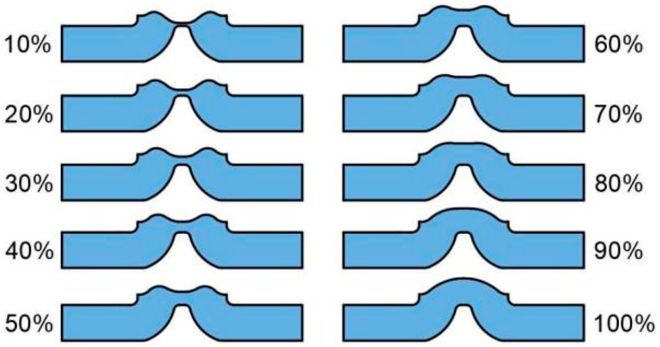
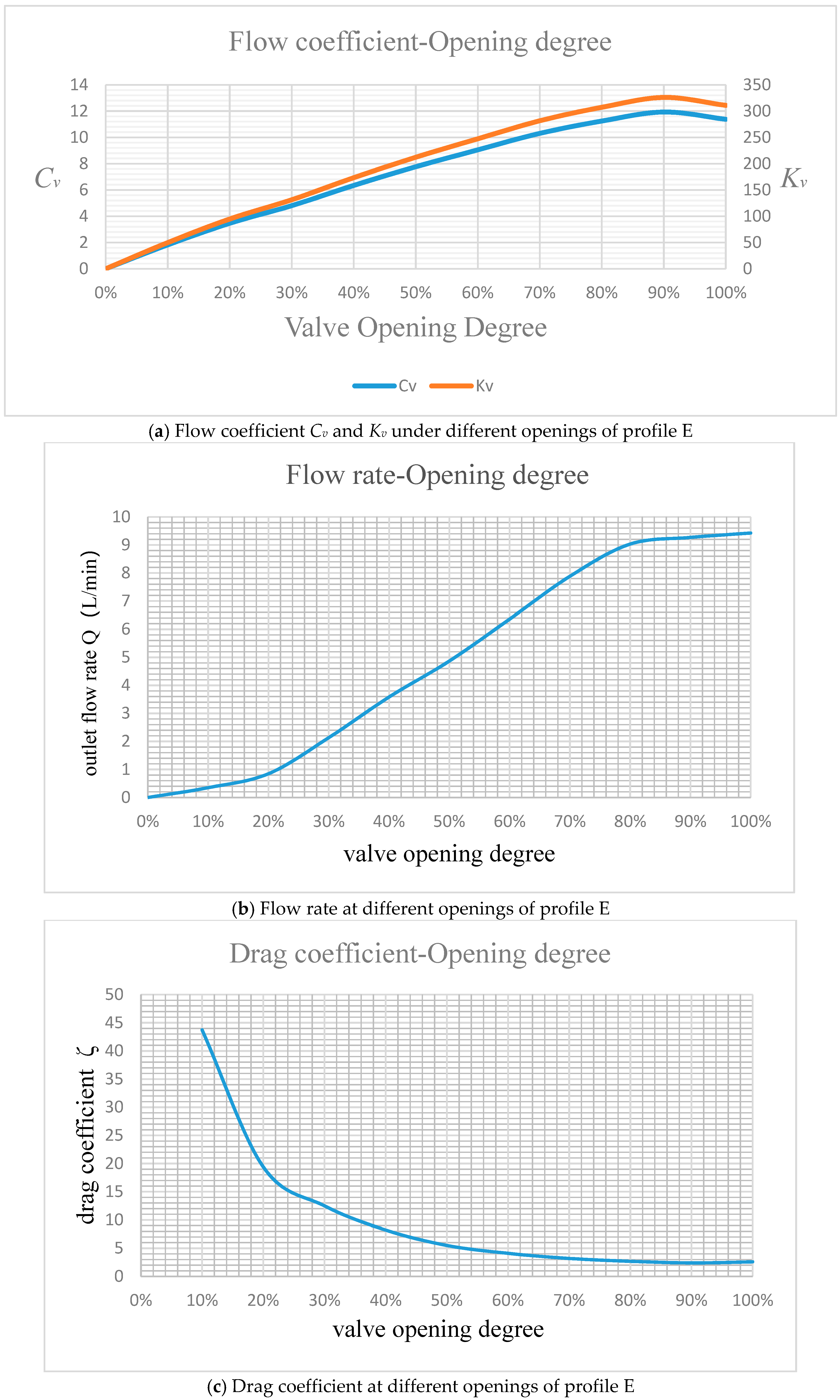
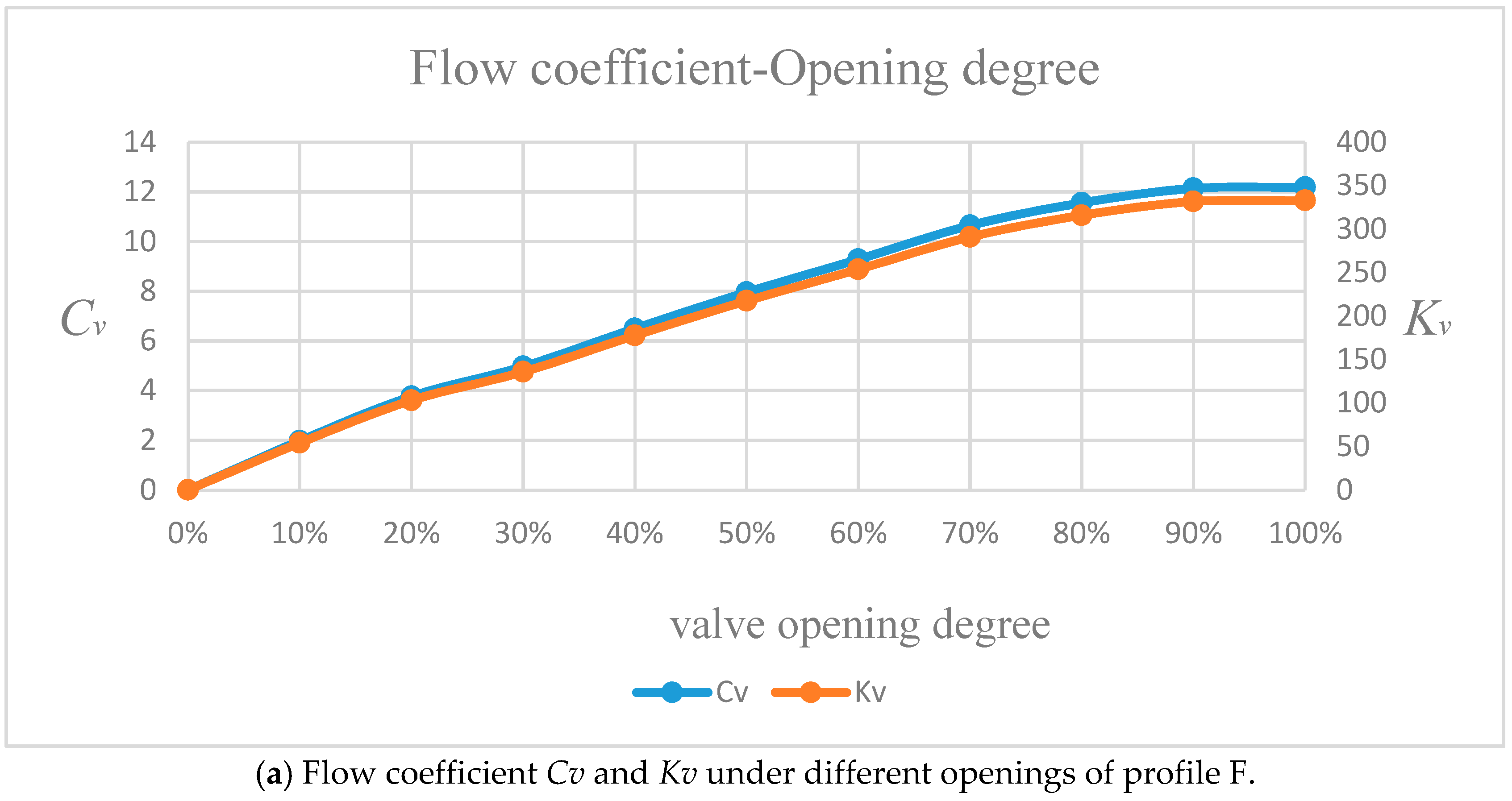
4.1. Throttling Characteristics

In general, the flow coefficients of profile B, C, and E decrease with the increase of flow velocity, which indicates that the greater the flow velocity, the greater the turbulent fluctuation, the more pressure loss is formed, which is in accordance with the general law (Figure 11). The flow coefficients of profile A increase obviously with the increase of Reynolds number, because the ridge of profile A is too steep and the flow velocity is lower. As a result of the blocking effect, it is not easy for the fluid to flow through the ridge. On the contrary, when the flow velocity is high, the fluid momentum is large and easy to pass, so the pressure drop decreases and the flow coefficient increases. The flow coefficient of profile d does not change obviously with the increase of Reynolds number. The possible reason is that the side of the ridge of profile d is gentle and easy for the fluid to pass through, but the width of the ridge top is wide. The narrow passage leads to an approximate sharp angle, which leads to an excessive bending angle of the flow passage, approaching 180 degrees. The fluid is not easy to turn, resulting in pressure loss. The two factors restrict each other, resulting in the flow coefficient almost unchanged.

By comparing the curves of profile A, B and C, it can be known that with the gradual increase of the flatness of the side wall of the ridge, the flow coefficient becomes larger and the flow performance is better at the same flow velocity; by comparing the curves of profile C, D and E, we can know that the appropriate increase of the width of the top of the ridge is beneficial to the fluid steering, flow passage and flow coefficient. The circulation performance is better. Therefore, the top of the ridge should be too narrow, and the side walls of the ridge should be too steep.

Comparing the streamline diagrams of four types of surfaces (Figure 12), it can be seen that there are large vortices near the right side of the ridge and the upper wall of the exit, which is the direct cause of pressure loss. The former is determined by the shape of the ridge, and the latter is caused by the protrusion of the pipe wall on the right side of the upper wall hindering the flow. In addition, there are small eddies on the edge of the diaphragm and valve body installation. In addition, although there are two large eddy zones, the shape and size of the eddy zones are also different. When the ridge is too steep or the ridge top is too narrow, leading to too large bending, the scale of the right-side eddy on the ridge is very large, and the shape of the eddy is nearly circular, resulting in a great pressure loss. In contrast, the right-side eddy zones of the ridge of B and E are relatively flat. It can be inferred that increasing the flatness of the side of the ridge can reduce the vortices to a certain extent; for the vortices near the upper wall at the exit, the roundness of the protrusion of the inner wall of the upper wall can be appropriately increased or a more suitable shape can be designed to weaken the vortices.

4.2. Opening and Closing Characteristics

According to the flow coefficient diagram (Figure 13a), with the increase of opening, the flow performance increases, pressure loss decreases, and flow coefficient increases. However, in the range of 80–100% opening, the flow coefficient has experienced a process of first rising and then falling, and the flow performance is the best around 90% opening (Figure 13b). By comparing the inner surface shapes of 80%, 90% and 100% open diaphragms, it can be seen that the central area of the inner surface of 90% open diaphragms is close to the plane, while the central area is concave when the valve orifice is fully open. It can be inferred that the flow performance is better when the central area of the inner surface of diaphragms is horizontal than that when the valve orifice is concave. It can be guessed that the central area will be approximately planar when the diaphragm is manufactured, or a 10% pre-clearance will be given when the diaphragm is installed to ensure the best flow performance when the diaphragm is fully open.

By analyzing the local resistance coefficient diagram (Figure 13c), we can know that the resistance effect of the valve is obvious when the valve is small. The relationship between outlet flow rate and valve opening shows that the linearity of the middle section of flow control is better but the linearity area is not large. In the two opening areas of 0–20% and 80–100%, the flow characteristics of the valve are not good. The reason is that the small opening can easily cause jet flow or even cavitation, and blocking flow is easy to occur, which results in a small flow variation range and a large flow rate. When opening, the throttling effect caused by the change of valve opening is not obvious and the flow control characteristics are not good because the diameter of valve opening is similar to the diameter of pipeline at the entrance of river basin. In the middle opening range, we can know that the flow characteristics are approximately linear, and the flow control performance is good.

4.3. Cavitation Characteristics

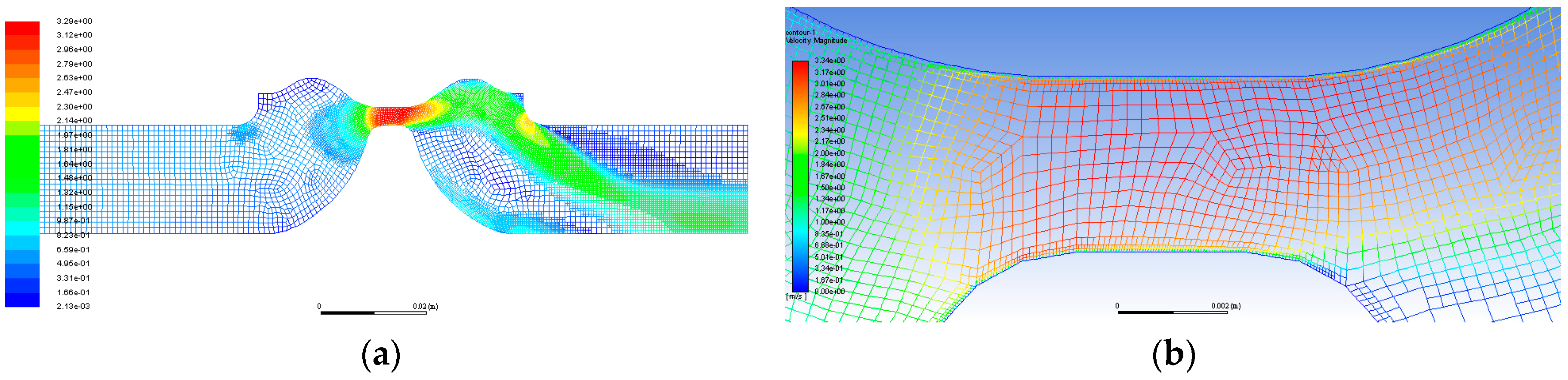
4.3.1. The Influence of Opening Degree

Under the given boundary conditions, cavitation begins to appear near the lower boundary of the valve orifice and the corner of the outlet bending when the opening of the diaphragm valve drops to 50%. With the opening decreasing, the cavitation area gradually expands and develops to the upper boundary of the valve orifice (Figure 14). When the opening is below 20%, the cavitation area shrinks to the valve orifice and cavitates near the corner of the outlet bending. When the opening is less than 10%, the cavitation area continues to shrink near the center of the valve opening.

4.3.2. Effect of Entrance Boundary Conditions (at 10% Opening)

The inlet is still set as pressure inlet, the setting value increases from p_in = 500 kPa to p_in = 100 kPa intervals, and the outlet is set as pressure outlet with p_out = 100 kPa back pressure. Two-phase volume fraction nephogram of observed time-averaged cavitation results can be obtained by processing and calculating the data of outlet flow rate, pressure difference at both ends and inlet flow rate, and the change of mass flow rate at both ends of inlet and outlet can be obtained with the increase of pressure boundary conditions (Figure 15).

The reason is that when the pressure difference between the two ends Δp is greater than 800 kPa, the cavitation phenomenon becomes serious and more cavitation bubbles are blocked at the valve mouth, which leads to flow saturation and deviates from the theoretical flow input. And Figure 16 shows a volume fraction nephogram at different inlet pressures.

4.4. Shape Optimization and Verification

According to the conclusion analysis of the influence of the structure of the runner profile on the throttling characteristics and the flow control characteristics, the following optimization ideas can be obtained: Increasing the lateral flatness of the ridge, appropriately increasing the width of the ridge top and reducing the protrusion of the inner wall of the valve at the diaphragm installation can increase the flow coefficient and reduce the local resistance coefficient of the valve, and appropriately reduce the diaphragm stroke, the central area of the inner surface of the diaphragm approximates the plane at the maximum opening, and give the diaphragm a pre-stroke during installation. The flow control characteristics of the diaphragm valve can be improved appropriately and the linear range of the flow control zone can be enlarged. The improvement of various surface structures should be carried out on the premise of ensuring the overall size ratio of diaphragm valves.

The optimized prototype is based on the well-behaved surface e, and further flattens the ridge ridge, reduces the obstacles at the protrusions, and modifies the shape of the inner surface of the diaphragm so that the central area of the inner surface of the diaphragm is planar in the fully open state, thus reducing the diaphragm travel. The comparison between the optimized profile F and profile E is shown in Figure 17.

The flow coefficient and local resistance coefficient (Figure 18) of the optimized profile are improved to a certain extent compared with the prototype profile E before optimization; with the increase of the opening of the profile F valve, the flow coefficient shows an increasing trend, and no longer decreases with the increase of the opening when approaching full opening (Figure 19a). In addition, some improvements have been made in the flow control characteristics of the valve under profile F. In addition to the good linearity, the linearity range has also been enlarged at large valve ports (Figure 19b).

As can be seen from the streamline diagram (Figure 20), the vortices on the right side of the ridge are compressed to a great extent, which hardly hinders the main flow. The vortices near the upper wall of the valve outlet are almost non-existent, indicating that the reduction of the flow path hindrance has a great effect on the reduction of the vortices.

5. Conclusions

The deformation mechanism of diaphragm valve diaphragm is analyzed and simulated by the finite element method. The influence of diaphragm thickness and the loading mode of stem loading on diaphragm deformation are explored. The conclusion is drawn that the diaphragm with thin and moderate loading area had better sealing and control characteristics. The effect of velocity gradient adaptive and y⁺ adaptive methods on mesh optimization in some regions and the effect of refined mesh on simulation accuracy are verified by means of mesh adaptive technology.

In the way of design comparison, the influence of the sill-shaped diaphragm structure on the flow coefficient and the drag coefficient of the valve is discussed. Combined with the simulation of the cloud map and the simulation of the flow field under different opening degrees of the valve, the optimized diaphragm flow is obtained. The theoretical idea of the pavement surface structure: smoothing the side wall of the ridge, increasing the width of the ridge, reducing the obstruction of the pipeline and smoothing the lower surface of the diaphragm. Optimize the design in this direction and further simulate to analyze the correctness of the verification optimization.

Through the analysis of gas-liquid two-phase flow nephogram, it is concluded that with the valve closing cavitation gradually occurs and expands, and with the increase of inlet boundary conditions, the small valve opening cavitation becomes more and more serious.

In this paper, the factors influencing the flow characteristics of diaphragm valves and the method of optimizing the flow profile are systematically studied. The main technical indexes of diaphragm valves, such as controllability, flow performance, diaphragm life, cleanliness, and sealing, are comprehensively studied. The improvement of Throttling Characteristics and control characteristics is beneficial to ultra-pure water system and submerged photolithography. The improvement of technology is of great benefit and constructive and forward-looking to the development of semiconductor industry.

References

1. Mbiya, B.M.; Fester, V.G.; Slatter, P.T. Evaluating resistance coefficients of straight through diaphragm control valves. Can. J. Chem. Eng. 2009, 10, 704–714. [Google Scholar] [CrossRef]
2. Cheng, Y.; Liu, M. Selection of common valves in chemical engineering design. Guangdong Chem. Ind. 2009, 8, 244–245. [Google Scholar]
3. Wu, H. Requirements for selection and installation of diaphragm valve in clean fluid conveying system. Chem. Pharm. Eng. 2016, 37, 50–54. [Google Scholar]
4. Nguyen, T.; van der Meer, D.; van den Berg, A.; Eijkel, J.C.T. Investigation of the effects of time periodic pressure and potential gradients on viscoelastic fluid flow in circular narrow confinements. Microfluid Nanofluid 2017, 21, 37. [Google Scholar] [CrossRef] [Green Version]
5. Jerman, J.H. Electrically-Activated, Micromachined Diaphragm Valves. Micro System Technologies 90; Springer: Berlin/Heidelberg, Germany, 1990; pp. 806–811. [Google Scholar]
6. Yang, F.; Imin, K. Analysis of fluid flow and deflection for pressure-balanced MEMS diaphragm valves. Sens. Actuators A Phys. 2000, 79, 13–21. [Google Scholar] [CrossRef]
7. Lin, B.J. Immersion lithography and its impact on semiconductor manufacturing. J. Micro/Nanolithogr. MEMS MOEMS 2004, 3, 377–501. [Google Scholar] [CrossRef]
8. Owa, S.; Nagasaka, H. Immersion lithography: its potential performance and issues. In Optical Microlithography XVI; International Society for Optics and Photonics: Bellingham, WA, USA, 2003; pp. 724–733. [Google Scholar]
9. Cao, F. Design and Implementation of the State Control of Immersion System of Immersion Lithography Machine based on DSL. Master’s Thesis, Zhejiang University, Hangzhou, Zhejiang, China, 15 January 2017. [Google Scholar]
10. Chen, W. Study on Liquid Supply and Sealing of Immersion Control Unit in Immersion Lithography. Master’s Thesis, Zhejiang University, Hangzhou, Zhejiang, China, 30 June 2010. [Google Scholar]
11. Kim, T.H.; Sunkara, V.; Park, J.; Kim, C.J.; Woo, H.K.; Cho, Y.K. A lab-on-a-disc with reversible and thermally stable diaphragm valves. Lab Chip 2016, 16, 3741–3749. [Google Scholar] [CrossRef]
12. Ohlsson, P.A. Diaphragm valve development–challenging traditional thinking. Pharm. Eng. 2013, 33, 1–4. [Google Scholar]
13. Tanikawa, T.; Yamaji, M.; Yakushijin, T.; Fukuchi, O. Direct Touch Type Metal Diaphragm Valve. U.S. Patent 8,256,744, 4 September 2012. [Google Scholar]
14. Lv, B. Practical Rubber Handbook; Chemical Industry Press: Beijing, China, 2009. [Google Scholar]
15. Jerman, H. Electrically-activated, normally-closed diaphragm valves. In Proceedings of the International Conference on Solid-State Sensors and Actuators, San Francisco, CA, USA, 24–27 June 1991; pp. 1045–1048. [Google Scholar]
16. Sun, X.; Gu, X.; Carr, W.N. Lateral in-plane displacement microactuators with combined thermal and electrostatic drive. In Proceedings of the 8th International Conference on Solid-State Sensors and Actuators and Eurosensors IX, Stockholm, Sweden, 25–29 June 1995. [Google Scholar]
17. Li, Y.; Sun, L. Manufacture and Application of Rubber Compound—FIuoroplastics Composite Diaphragm for Pumps and Valves. Spec. Purp. Rubber Prod. 2010, 31, 35–38. [Google Scholar]
18. Lu, P. Practical Valve Design Manual; Machinery Industry Press: Beijing, China, 2012. [Google Scholar]
19. Cui, B.; Ma, G.; Wang, H.; Lin, Z. Influence of valve core structure on flow resistance characteristics and internal flow field of throttling stop valve. J. Mech. Eng. 2005, 51, 178–184. [Google Scholar] [CrossRef]
20. Zhang, Y. Hydromechanics; Higher Education Press: Beijing, China, 2016. [Google Scholar]
21. Cai, S. Diaphragm flow regulating valve. China Pet. Mach. 2006, 2, 31–32. [Google Scholar]
22. Fester, V.G.; Kazadi, D.M.; Mbiya, B.M.; Slatter, P.T. Loss coefficients for flow of Newtonian and non-Newtonian fluids through diaphragm valves. Chem. Eng. Res. Des. 2007, 85, 1314–1324. [Google Scholar] [CrossRef]
23. Wang, Z. Research on Flow Field Simulation and Optimum Design Method for Process Valve. Master’s Thesis, University of Electronic Science and Technology of China, Chengdu, Sichuan, China, 19 June 2017. [Google Scholar]
24. Wu, D.; Li, S.; Wu, P. CFD simulation of flow-pressure characteristics of a pressure control valve for automotive fuel supply system. Energy Convers. Manag. 2015, 101, 658–665. [Google Scholar] [CrossRef]
25. Liu, X.; Liu, Y.; Guo, X.; Zhang, K. Research on the simulation of inflow control valve based on FLUENT. Mech. Eng. 2018, 10, 3–6. [Google Scholar]
26. Zhang, J.; Wang, D.; Xu, B.; Gan, M.Y.; Pan, M.; Yang, H.Y. Experimental and numerical investigation of flow forces in a seat valve using a damping sleeve with orifices. J. Zhejiang Univ. Sci. A 2018, 19, 417–430. [Google Scholar] [CrossRef]
27. Qian, J.; Gao, Z.; Liu, B.; Jin, Z.J. Parametric study on fluid dynamics of pilot-control angle globe valve. J. Fluids Eng. 2018, 140, 111103. [Google Scholar] [CrossRef]
28. Ye, S.; Zhang, J.; Xu, B.; Zhu, S.; Xiang, J.; Tang, H. Theoretical investigation of the contributions of the excitation forces to the vibration of an axial piston pump. Mech. Syst. Signal Process. 2019, 129, 201–217. [Google Scholar] [CrossRef]
29. Qian, J.; Chen, M.; Liu, X.; Jin, Z.J. A numerical investigation of the flow of nanofluids through a micro Tesla valve. J. Zhejiang Univ. Sci. A 2019, 20, 50–60. [Google Scholar] [CrossRef]
30. Zhou, X.; Wang, Z.; Zhang, Y. Flow Coefficient calculation method based on CFD and mesh adaptive method. J. Univ. Electron. Sci. Technol. 2017, 2, 475–480. [Google Scholar]
31. Javorik, J.; Stanek, M. The numerical simulation of the rubber diaphragm behavior. Situations 2011, 3, 4. [Google Scholar]
32. He-xiang, W.; Yong-ming, W.; Jia-zhen, P. Optimizing the configuration of the diaphragm valve film by ANSYS. Mech. Res. Appl. 2009, 3, 63–64. [Google Scholar]
Figure 1. Shape and size of the diaphragm with three kinds of the stem loading surface parameter.
Processes 07 00671 g001
Figure 2. Numerical model of the diaphragm (a) the model mesh with a diaphragm thickness of B0 = 6 mm and (b) the total deformation of the diaphragm with a thickness of B0 = 4 mm.
Processes 07 00671 g002
Figure 3. Displacement Diagram and Stress Diagram of Diaphragms with Different Thicknesses.
Processes 07 00671 g003
Figure 4. Diaphragm Deformation under Different Loading Area.
Processes 07 00671 g004
Figure 5. Working Principle of Weir Diaphragm Valve.
Processes 07 00671 g005
Figure 6. Flow Path Structure Dimensions and Five Ridge Profiles.
Processes 07 00671 g006
Figure 7. The two-dimensional flow field model of valve at different openings (profile E).
Processes 07 00671 g007
Figure 8. Mesh of different sizes under profile E. (a) for 0.5 mm; (b) for 1 mm; (c) for 2 mm.
Processes 07 00671 g008
Figure 9. Cloud Map Display of Velocity Field at Different Openings shows that as the valve opening decreases, the velocity gradient increases. (a) for 40% opening; (b) for 30% opening; (c) for 20% opening; (d) for 10% opening.
Processes 07 00671 g009
Figure 10. The meshes of three-time velocity adaptation (a) velocity gradient and y+ hybrid adaptation; (b) and their results of calculation (Table 2 and Table 3), respectively.
Processes 07 00671 g010
Figure 11. The results of the Comparison of Throttling Characteristics of Five Profiles. (a) Cv-Re of five different ridge profiles; (b) ζ-v of five different ridge profiles.
Processes 07 00671 g011
Figure 12. The streamline diagrams of four types of surfaces.
Processes 07 00671 g012
Figure 13. The results of the flow characteristics at different openings of profile E.
Processes 07 00671 g013
Figure 14. Volume fraction α of two phases and void fraction distribution of cavitation phase in valve flow field.
Processes 07 00671 g014aProcesses 07 00671 g014b
Figure 15. With the increase of inlet pressure, the inlet flow rate and outlet flow rate increase almost linearly, but when the inlet pressure pin increases to more than 900 kPa, the increase of outlet flow rate slows down, resulting in a larger flow loss.
Processes 07 00671 g015
Figure 16. Volume fraction nephogram at different inlet pressures.
Processes 07 00671 g016aProcesses 07 00671 g016b
Figure 17. The optimized surface F and the optimized surface E.
Processes 07 00671 g017
Figure 18. Comparison on flow characteristics (a) and drag characteristics (b) between profile E and the optimized profile F.
Processes 07 00671 g018
Figure 19. The results of the flow characteristics at different openings of profile F.
Processes 07 00671 g019aProcesses 07 00671 g019b
Figure 20. Streamline diagram of profile F at full opening.
Processes 07 00671 g020