Intelligent Energy Management for Plug-in Hybrid Electric Bus with Limited State Space

Abstract

Tabular Q-learning (QL) can be easily implemented into a controller to realize self-learning energy management control of a plug-in hybrid electric bus (PHEB). However, the “curse of dimensionality” problem is difficult to avoid, as the design space is huge. This paper proposes a QL-PMP algorithm (QL and Pontryagin minimum principle (PMP)) to address the problem. The main novelty is that the difference between the feedback SOC (state of charge) and the reference SOC is exclusively designed as state, and then a limited state space with 50 rows and 25 columns is proposed. The off-line training process shows that the limited state space is reasonable and adequate for the self-learning; the Hardware-in-Loop (HIL) simulation results show that the QL-PMP strategy can be implemented into a controller to realize real-time control, and can on average improve the fuel economy by 20.42%, compared to the charge depleting–charge sustaining (CDCS) strategy.

1. Introduction

Plug-in hybrid electric vehicle (PHEV) is a promising approach for energy-saving and lowering emissions, which would help the problems of energy shortage, global warming, and environment pollution [1]. Moreover, the advantage of the PHEV can be maximized by a well-designed energy management strategy (EMS) [2].

Rule-based control strategy is one of the most widely used methods in real-world situation, due to its easy implementation and real-time control performances [3]. Moreover, many investigations have demonstrated that the blended charge depletion (BCD) mode is the most efficient strategy, namely, the SOC can continuously decline to the expected value (such as 0.3) at the destination of route [4,5]. However, known driving conditions are usually indispensable for the BCD strategy, which brings great challenge to practical application.

Since the EMS can be taken as a nonlinearly constrained optimization control problem, the BCD mode can be well realized by optimal control methods [6]. It can be further classified into two categories: The optimization-based and the adaptive strategies [7]. The optimization-based strategies, such as dynamic programming (DP), Pontryagin’s Minimum Principle (PMP), and Equivalent Consumption Minimization Strategy (ECMS), can obtain global optimization solutions [8,9,10]. However, driving conditions need to be known prior to use, which is the reason that they cannot be directly used in real-world situations and are usually only taken as the benchmark for other strategies. In contrast, the adaptive strategy has great potential in practical application [7]. For example, a model predictive control (MPC)-based EMS was proposed by combining Markov chain, DP, and a reference SOC plan method, based on the principle of receding horizon control [11]. An Adaptive PMP (A-PMP)-based-EMS was proposed by combining PI, PMP, and reference SOC plan method, based on the principle of feedback control [12]. An Adaptive ECMS (A-ECMS)-based-EMS was proposed by combining ECMS and particle swarm optimization (PSO) algorithms, where the equivalent factors (EFs) were firstly optimized, and then the actual EF was recognized based on a look-up table constituted by the optimized EFs [13]. A driving pattern recognition-based EMS was proposed based on PSO algorithm, where a series of typical reference cycles were firstly optimized off-line, then the corresponding optimal results were taken as the sampling sets for real-time control [14].

Reinforcement learning (RL) is an intelligent method that can be used in EMS, where Q-learning (QL) is the most popular method. It can be further classified into tabular and deep learning methods. The former can easily solve the self-learning problem, by employing a simplified Q-table. However, the state and the action should be discretized and the “curse of dimensionality” problem may be introduced once the state space is huge. In contrast, the Q-table will be substituted by neural network (NN) in the deep learning-based-EMS, and the control problem with continuous variable can also be solved. For the former, Ref. [15] proposed a Tabular QL-based EMS, where the required power, the velocity, and the SOC were taken as the states, meanwhile, the current of the battery and the shifting instruction of the automated mechanical transmission (AMT) were taken as the actions. Ref. [16] proposed a similar method by employing a Markov chain and a Kullback–Leibler (KL) divergence rate, where the power, the SOC and the state of voltage (SOC) were taken as the states, meanwhile, the current of the battery was taken as the action. Ref. [17] proposed a different Tabular QL-based EMS, where the SOC and the speed of the engine were taken as the states, and the throttle of the engine was taken as the action. For the latter, Ref. [18] proposed a deep QL (DQL)-based EMS based on NN, where the SOC, the engine power, the velocity and the acceleration were taken as the states, and the increment of the engine power was taken as the action. Ref. [19] proposed a similar DQL method, where the required torque and the SOC were taken as the states, and the engine torque was taken as the action. Ref. [20] proposed a different DQL-based EMS with AC (action–critic) framework, where the speed together with the torque of the wheel, the SOC together with the voltage of the battery, and the gear position of the AMT were taken as the states, meanwhile, the power of the motor was taken as the action. Ref. [21] proposed an interesting DQL-based EMS using a neural network, where the required power at the wheels, the SOC together with the distance to destination were taken as the states, and the power of the engine was taken as the action. Nevertheless, the existing tabular QL based-methods usually have huge state space, which is easy to result in the “curse of dimensionality” problem. On the other hand, the control performance of the DQL method may be greatly deteriorated once the fitting precision of NN is low. Moreover, the high computation burden of the deep learning may also restrict its application in currently used controllers.

This paper aims at solving the practical application problem of self-learning energy management for a single-parallel plug-in hybrid electric bus (PHEB). Since the shift instruction (discrete variable) and the throttle of the engine (continuous variable) can simultaneously influence the fuel economy of the vehicle, a mixed control variable with compact format is deployed into the control strategy. The main innovation of this paper is that a QL-PMP-based EMS is proposed, by combining the QL and the PMP algorithms, where the mixed control variables can be indirectly solved by the PMP using a self-learned co-state from the QL. More importantly, since the co-state is mainly dependent on the difference between the feedback SOC and the reference SOC, a limited state space with 50 rows and 23 columns is designed. Because the state space is greatly reduced, the QL-PMP algorithm can be directly implemented into controller.

The remainder of this paper is structured as follows. The configuration, parameters and models of the PHEB are described in Section 2. The QL-PMP algorithm is formulated in Section 3. The training process is discussed in Section 4. The Hardware-in-Loop (HIL) simulation results are detailed in Section 5, and the conclusions are drawn in Section 6.

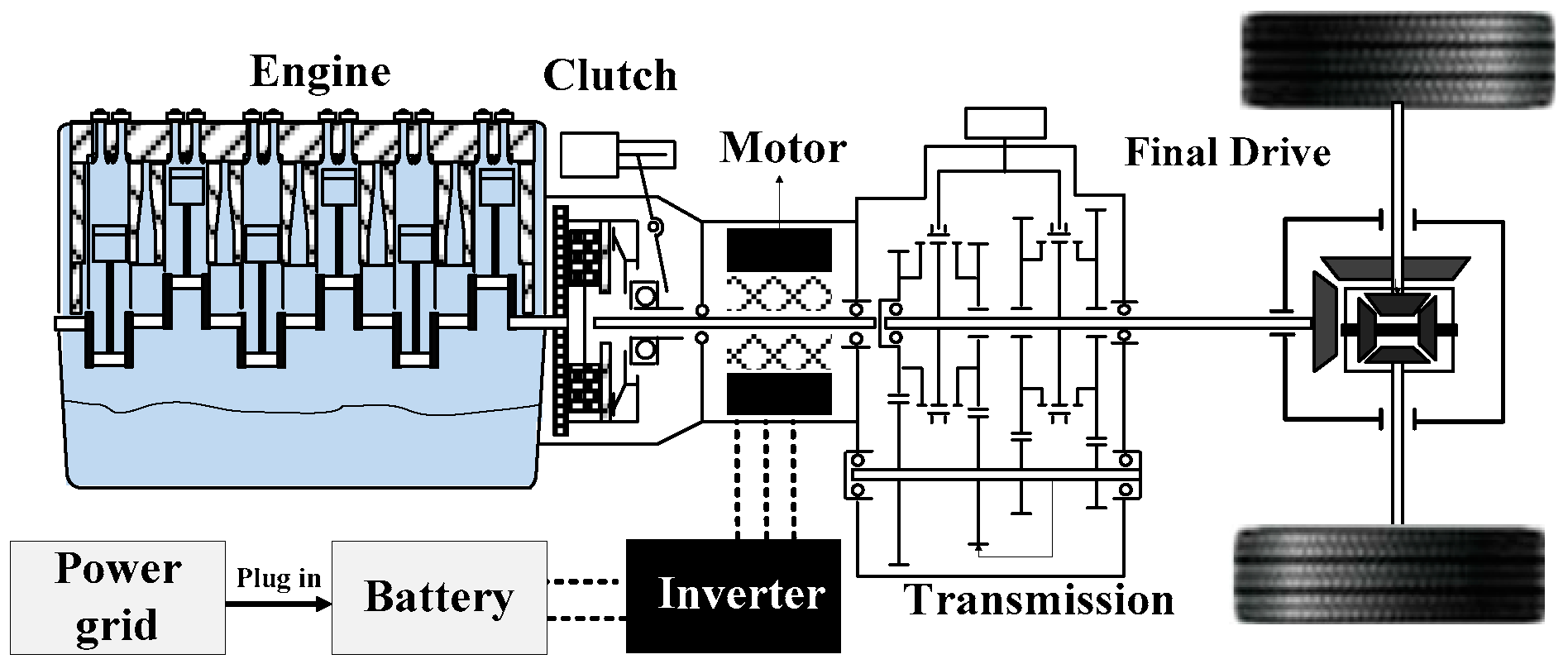
2. The Configuration, Parameters, and Models of the PHEB

The single-parallel PHEB is shown in Figure 1, which includes an engine, a motor, an AMT, a clutch, and a battery pack.

The engine and the motor will work coordinately to provide the required power of the PHEB, and the battery pack is the energy source for the motor. The clutch can change the driving modes during the vehicle runs. In specific, the regenerative braking and the pure electric driving modes can be realized when the clutch is disengaged, otherwise, the hybrid driving with or without charging mode can be realized. In addition, the detailed parameters of the PHEB are shown in

Table 1. The parameters of the PHEB. AMT: automated mechanical transmission.

Item	Description
Vehicle	Curb mass (kg): 8500
Passengers	Maximum number: 60; Passenger’s mass (kg): 70
AMT	Speed ratios: 4.09:2.45:1.5:0.81
Final drive	Speed ratio: 5.571
Engine	Max torque (Nm): 639
	Max power (kW): 120
Motor	Max torque (Nm): 604
	Max power (kW): 94
Battery	Capacity (Ah): 35

.

2.1. Modeling the Engine

The modeling of the engine can be classified into theoretical and empirical methods. The former is formulated by combustion, fluid mechanics, and dynamic theories. As shown in Figure 2, the instantaneous fuel consumption of the engine can be interpolated by the brake specific fuel consumption (BSFC) map, based on Equation (1).

$${\dot{m}}_e=\frac{T_e\cdot {\omega }_e\cdot b_e\cdot \Delta t}{\mathrm{3,600,000}}$$

(1)

where ${\dot{m}}_e$ denotes the instantaneous fuel consumption of the engine; $T_e$ denotes the torque of the engine; ${\omega }_e$ denotes the rotational speed of the engine; $b_e$ denotes the fuel consumption rate of the engine, which can be obtained by the speed and torque of the engine; $\Delta t$ denotes the sampling time.

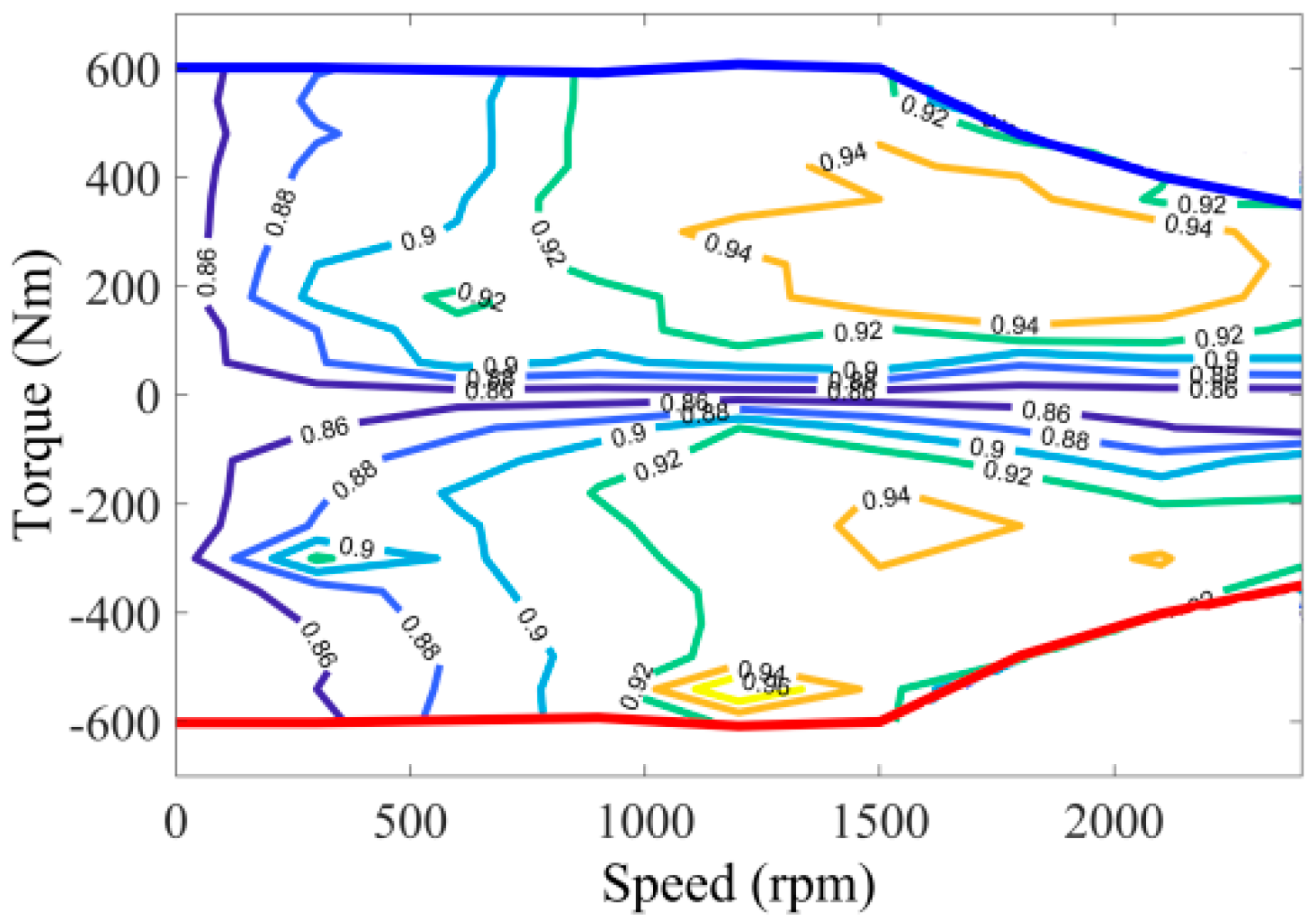
2.2. Modeling the Motor

Since only the working efficiency of the motor is need for the EMS, the empirical modeling method is adequate for the motor. In addition, because the motor can work in driving or regenerative mode, the motor model can be described as

$$P_m=\{\begin{array}{ll}{T}_m\cdot {\omega }_m/{\eta }_m& T_m>0\\ T_m\cdot {\omega }_m\cdot {\eta }_g& T_m\le 0\end{array}$$

(2)

where $P_m$ denotes the power of the motor, $T_m$ denotes the torque of the motor, ${\omega }_m$ denotes the rotational speed of the motor, and ${\eta }_m$ and ${\eta }_g$ denote the efficiency of the motor in driving mode and braking mode. When $T_m>0$, motor works in driving mode, and when $T_m\le 0$, motor works in braking mode. As shown in Figure 3, the power of the motor can be interpolated by the efficiency map of the motor, based on Equation (2).

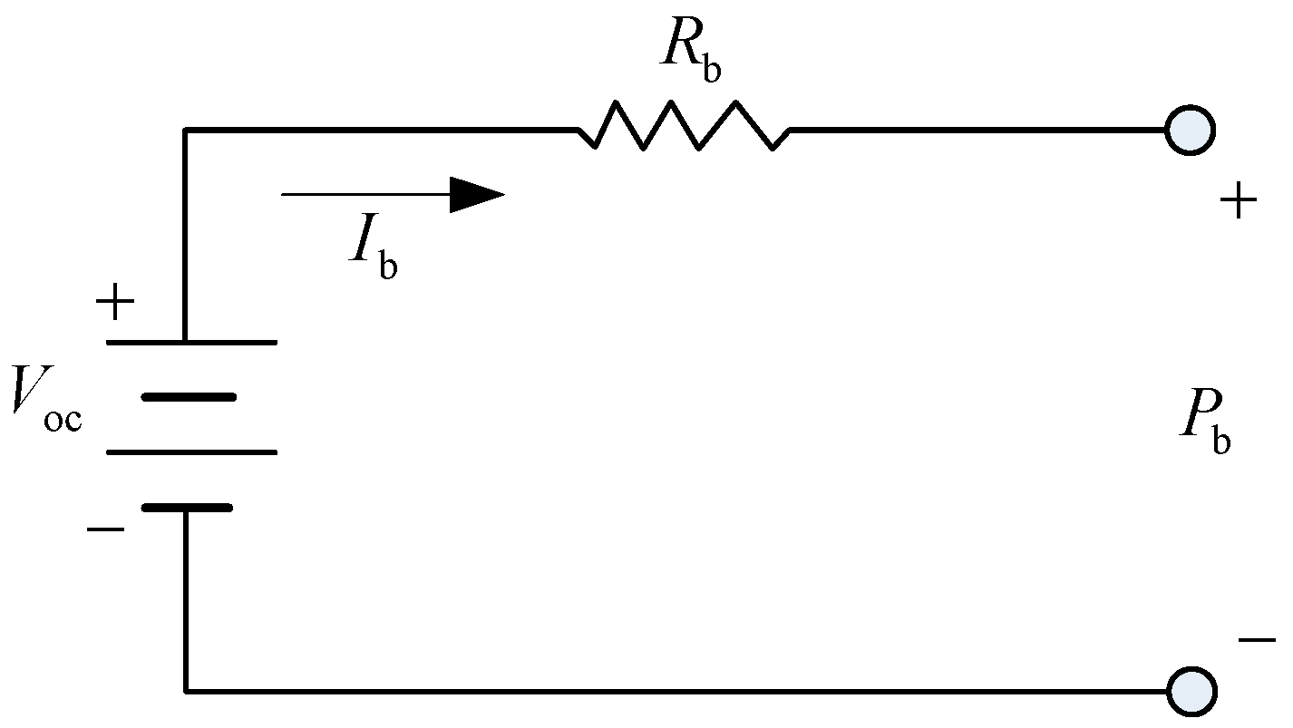
2.3. Modeling the Battery

For the energy management, the key issue of the battery is the estimation of the SOC, based on the voltage, the internal resistance and the current of the battery. Accordingly, a simplified battery model is deployed in Figure 4, and the power of the battery can be described as:

$$P_b=V_{oc}{I}_b-I_b^2{R}_b$$

(3)

where $P_b$ denotes the power of the battery, $V_{oc}$ denotes the open-circuit voltage of the battery, $I_b$ denotes the current of the battery and $R_b$ denotes the internal resistance of the battery.

2.4. The Dynamic Model of the Vehicle

Since only the required power is needed for the EMS, the model can be simplified to a lumped mass model, and only the longitudinal dynamic characteristic can be considered. Here, the driving and resistance forces can be described as:

$$F_t-F_R=\delta m\frac{\mathrm{d}v}{\mathrm{d}t}$$

(4)

where $F_t$ denotes the driving force, $\delta$ denotes the rotating mass conversion factor, and $m$ denotes the vehicle mass, which is constituted by the curb mass of the vehicle and the stochastic mass of the passengers, $F_R$ denotes the resistance force, which is constituted by:

$$F_R=fmg\cos {\alpha }_s+mg\sin {\alpha }_s+\frac{1}{2}{C}_D{A}_a{\rho }_a{v}^2$$

(5)

where $f$ denotes the coefficient of the rolling resistance, $g$ denotes the gravity acceleration, ${\alpha }_s$ denotes the road slope, $C_D$ and $A_a$ denote the coefficient of the air resistance and frontal area, respectively, ${\rho }_a$ denotes the air density, and $v$ denotes the velocity. The required power can be obtained by:

$$P_r=\frac{F_t\cdot v}{3600{\eta }_t}$$

(6)

where $P_r$ denotes the required power and ${\eta }_t$ denotes the efficiency of the transmission system.

3. The Formulation of the QL-PMP Algorithm

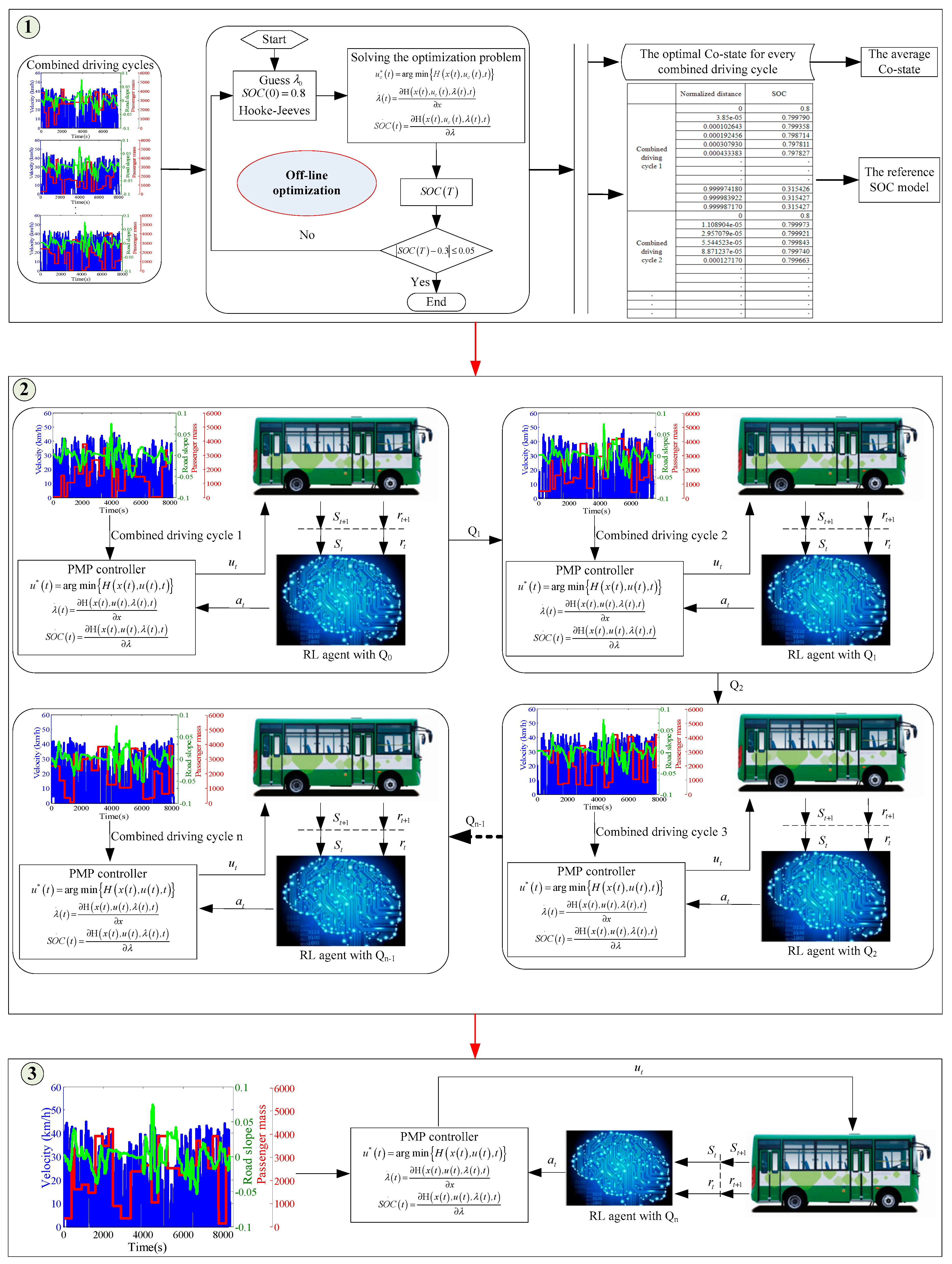
Different from the general traffic environment, the route of the PHEB is fixed and repeatable. Therefore, a series of historical driving cycles can be downloaded from remote monitoring system (RMS). In addition, many investigations have demonstrated that the factors of the velocity and the road slope have great effect on the EMS, which essentially points at the importance of the required power of the vehicle [2,7]. In this case, the factor of the stochastic vehicle mass is also a significant factor for EMS based on the Equations (4)–(6). Accordingly, a series of combined driving cycles constituted by the historical driving cycles, the road slope and the stochastic distributions of the vehicle mass are firstly designed. As shown in Figure 5, the training of the QL-PMP requires three steps.

Step 1

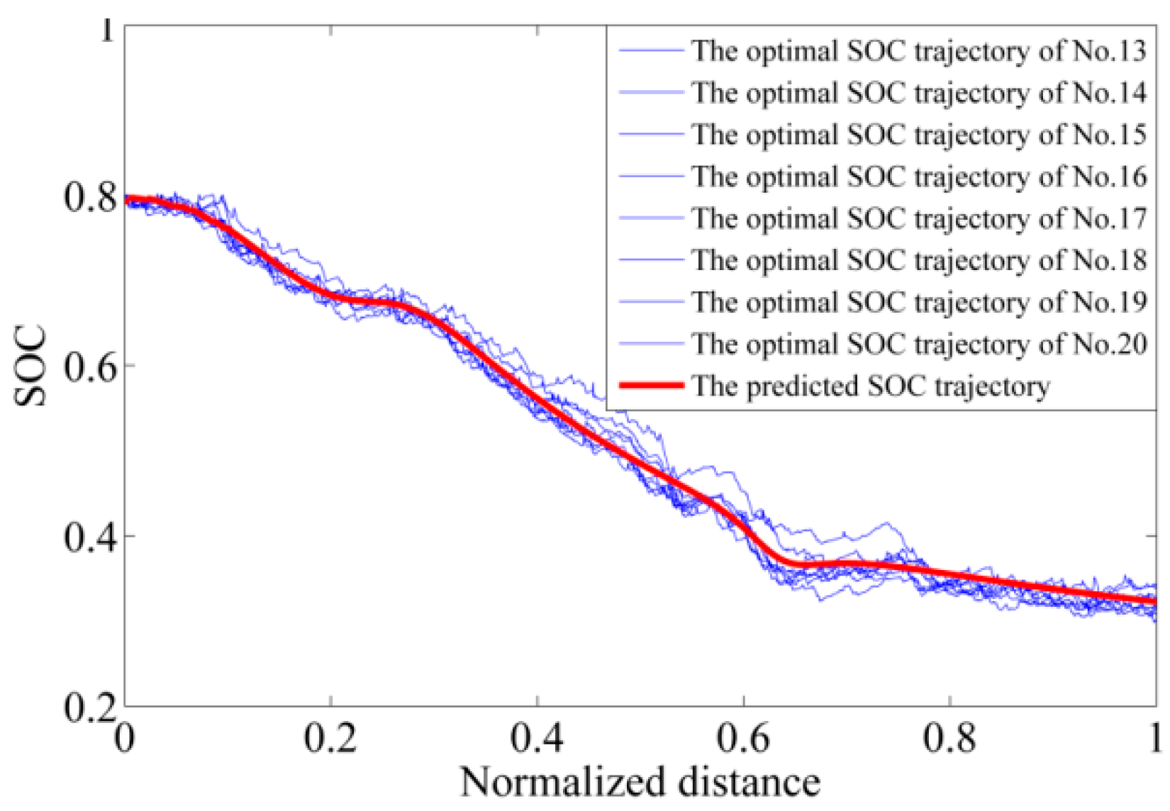
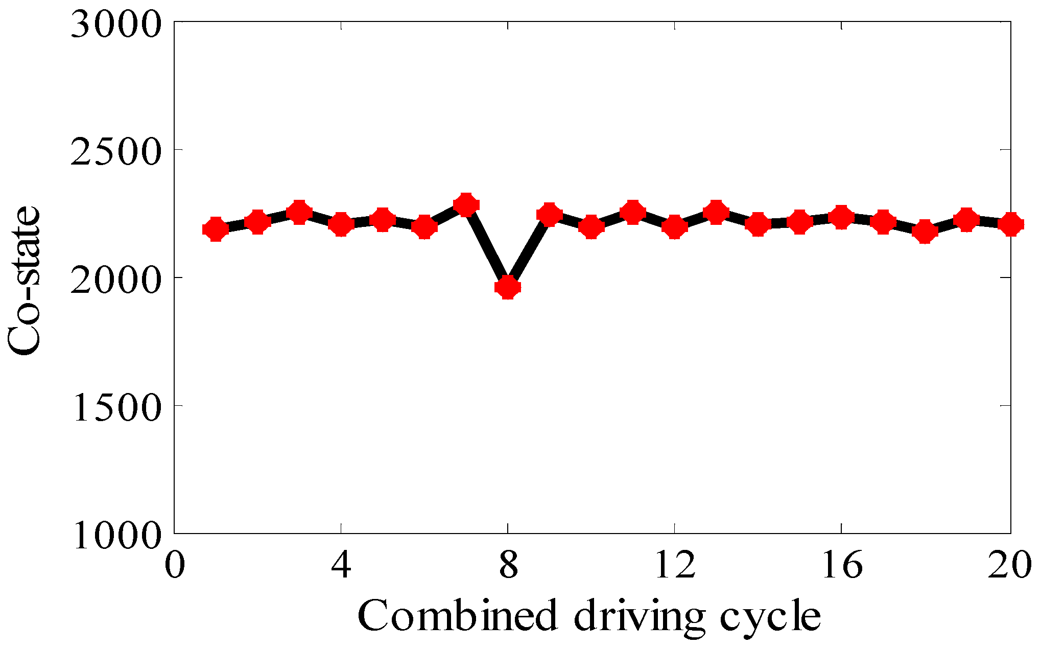
A series of co-states with respect to the combined driving cycles are firstly optimized, by an off-line PMP with Hooke–Jeeves algorithm [22]. Then, the average co-state is obtained and the corresponding optimal SOCs are extracted. Finally, a reference SOC model is established by taking the normalized distance as input and the optimal SOCs as output.

Step 2

Based on the known average co-state and the reference SOC model, the training of the QL-PMP is carried out as follows: firstly, the Q-table (denoted by Q₀), that is defined as zeros matrix, will be trained with the combined driving cycle 1; secondly, the trained Q-table (denoted by Q₁) will be taken as the initial Q-table for the second training with the combined driving cycle 2; and then this process will be continued until the Q-table is adequately trained.

Step 3

Verifying the adequately trained QL-PMP algorithm with HIL platform, using different combined driving cycles.

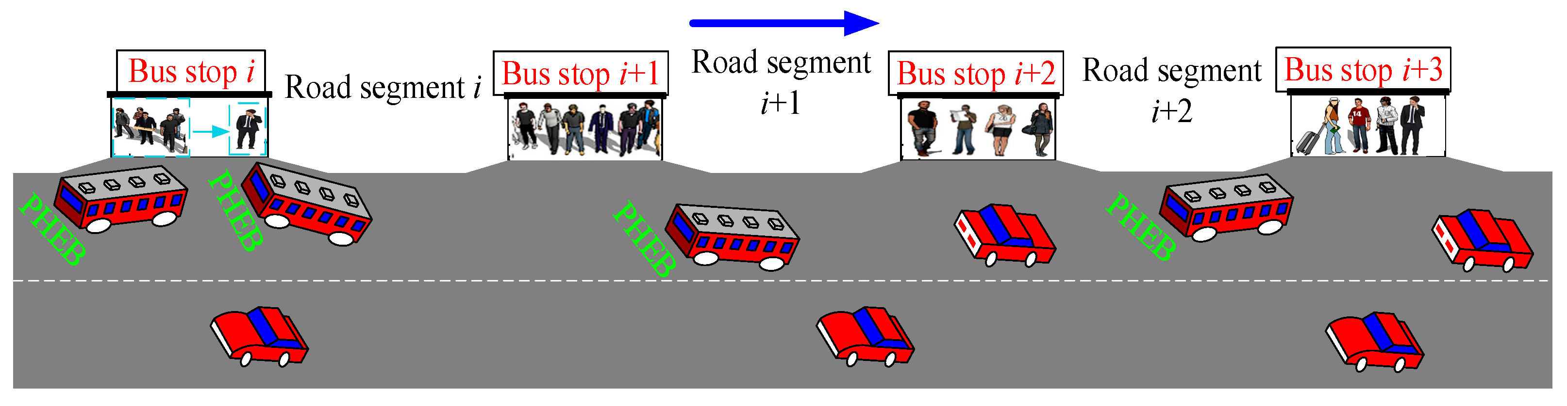
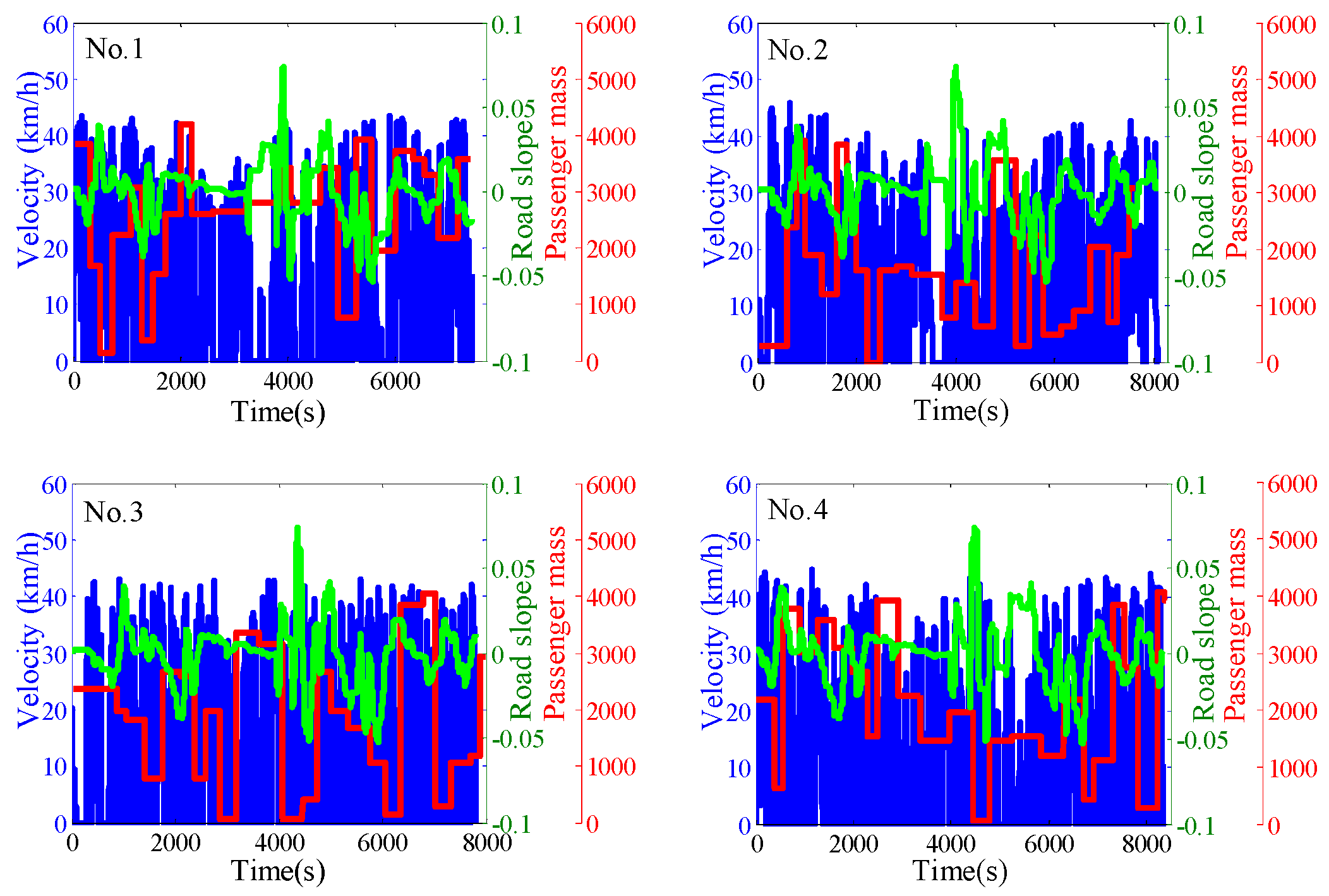
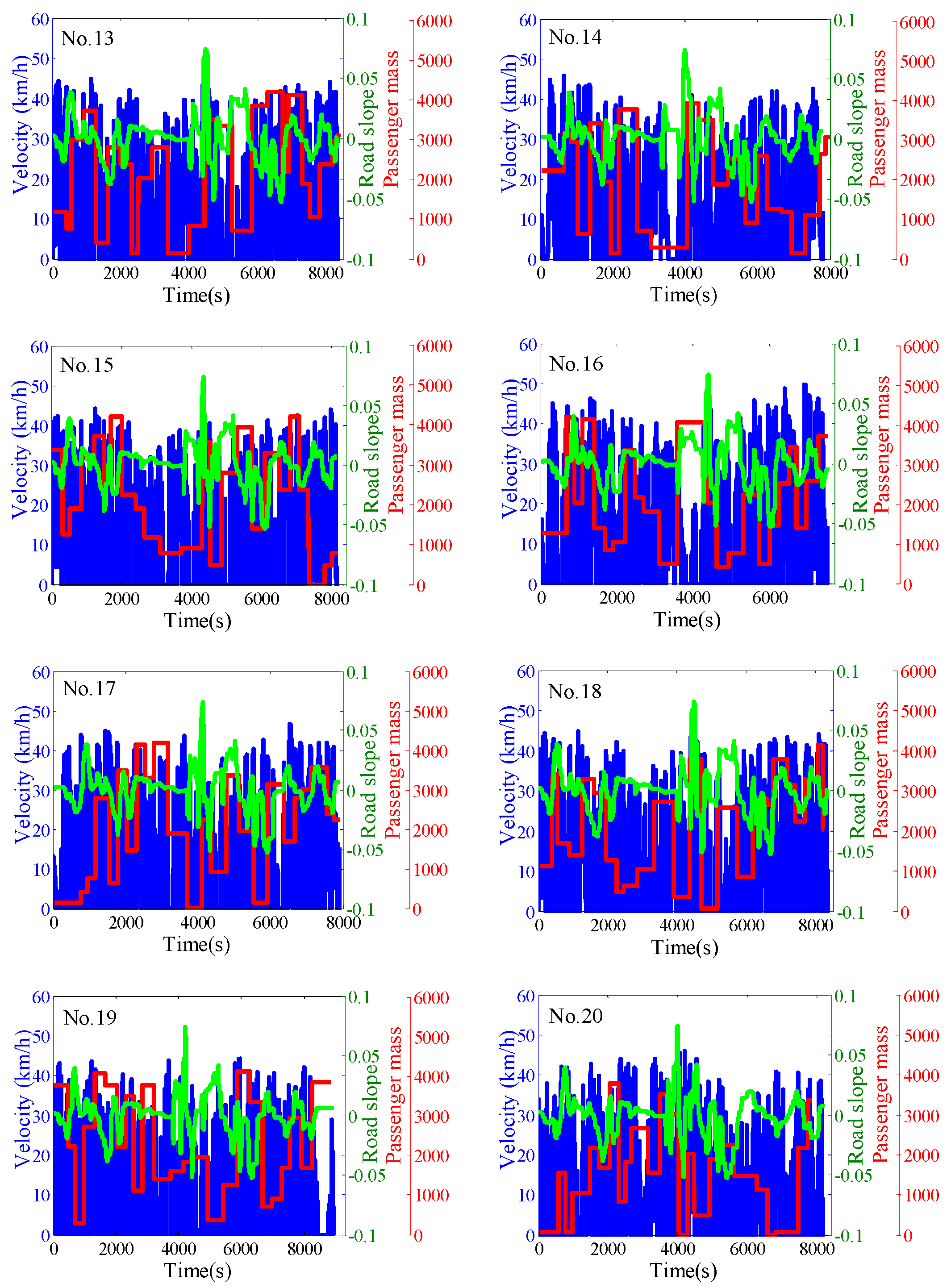
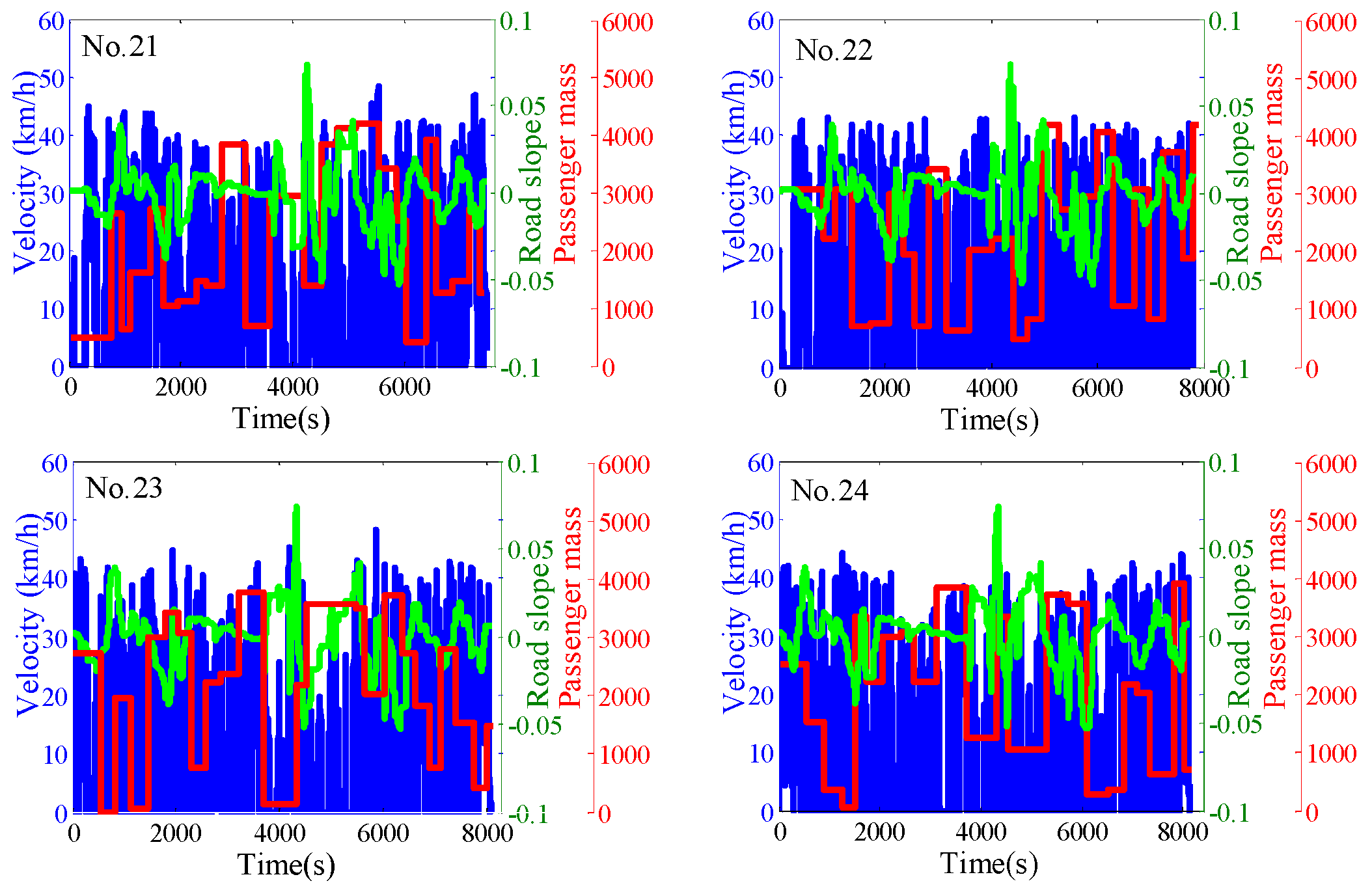
3.1. The Combined Driving Cycle

In terms of the combined driving cycle, the historical driving cycle can be downloaded from the RMS, and the road slope can be obtained off-line based on the attitude of the road and the corresponding travelled distance. To simplify the EMS problem, the road slope is implemented into the controller in a prior process by designing a look-up table, through taking the travelled distance as input and the road slop as output. Similar to Ref. [23], the stochastic distributions of the vehicle mass were designed as follows:

Firstly, as shown in Figure 6, 25 road segments are defined based on the number of the neighbored bus stops. Because the distributions of the passenger in different road segments are stochastic, 25 factors with respect to the road segments were defined to describe the stochastic distribution of the vehicle mass over the bus route.

Secondly, assuming the stochastic distribution of the vehicle mass is reflected by the passenger mass, 60 levels are defined for each factor, based on the maximum passenger number. Moreover, to exhaustively probe the design space constituted by the 25 factors, the Optimal Latin hypercube design (Opt. LHD) is deployed, due to its good spatial filling and equalization performances. Finally, the combined driving cycles are constructed by stochastic matching of the historical driving cycles, the road slope and the stochastic distributions of passenger mass (kg) are generated. As shown in Figure 7, the blue line represents the velocity of the PHEB, the red line represents the total mass of passengers, and the green line represents the slope of the road. Besides, the stochastic vehicle mass is added by the curb vehicle mass and the stochastic distribution of passenger mass.

3.2. The Off-Line PMP Algorithm

Theoretically, EMS can be taken as an optimal control problem, which can make the vehicle reach the optimal state within a time domain through a series of discrete controls. Furthermore, since the bus route is fixed, and the BCD mode can be realized by the optimal control, and the terminal SOC can be easily controlled within the expected zone. This implies that the terminal SOC may be similar, despite of any combined driving cycle. Therefore, the electricity consumptions of the battery are similar for all of the combined driving cycles, and the minimum fuel consumption of the PHEB can be taken as one of the objectives. Moreover, the shift number should also be restricted to improve the control performance. In addition, only the state of the SOC is selected to simplify the control problem, and the control vector is reduced to a one-dimensional format constituted by the shift instruction of the AMT and the throttle of the engine, then the optimal control problem of the energy management can be described as:

$$\begin{array}{l}\min J={\displaystyle {\int }_{t_0}^{t_f}{\dot{m}}_e}\left(u(t)\right)+\beta \left|s(t)\right|\mathrm{d}t\\ \mathrm{S}.\mathrm{t}.\{\begin{array}{l}S\dot{O}C(t)=-\frac{V_{oc}-\sqrt{V_{oc}^2-4R_{bat}{P}_{bat}}}{2R_{bat}{Q}_{nom}}\\ {\omega }_{e\_min}\le {\omega }_e(t)\le {\omega }_{e\_max}\\ {\omega }_{m\_min}\le {\omega }_m(t)\le {\omega }_{m\_max}\\ p_{e\_min}\le p_e(t)\le p_{e\_max}\\ p_{m\_min}\le p_m(t)\le p_{m\_max}\end{array}\end{array}$$

(7)

where $J$ denotes the performance index function; $u\left(t\right)$ (Equation (8)) denotes the control vector, which is defined as a compacted format and is sampled by Opt. LHD. Here, the shift instruction is denoted by $s\left(t\right)$, and the throttle of the engine is denoted by $th\left(t\right)$. Moreover, $s\left(t\right)$ is defined as −1, 0 and 1, denoting the downshift, hold on and upshift, respectively; $th\left(t\right)$ is ranged from 0 to 1.

$$u\left(t\right)=\left[\begin{array}{l}s\left(t\right)\\ th\left(t\right)\end{array}\right]$$

(8)

where the required power of the vehicle can be defined as $P_r$, $s\left(t\right)$ and $th\left(t\right)$ are changed with the state of $P_r$. If $P_r>0$, it means that the vehicle runs in the driving state, the AMT can carry out the controls of the downshift, hold on and upshift, and the throttle of the engine can be ranged from 0 to 1; if $P_r=0$, it means that the vehicle runs in the stopping state, the AMT will be downshifted to the lowest gear and the throttle of the engine is 0; if $P_r<0$, the vehicle runs in the braking state, the gear of the AMT will be maintained and the throttle of the engine is 0.

In addition, $S\dot{O}C\left(t\right)$ denotes the state function, $Q_{nom}$ denotes the battery capacity, ${\omega }_e\left(t\right)$ and ${\omega }_m\left(t\right)$ denote the rotate speeds of the engine and the motor, respectively, meanwhile, ${\omega }_{e\_min}$, ${\omega }_{e\_max}$ and ${\omega }_{m\_min}$, ${\omega }_{m\_max}$ denote the corresponding rotate speed boundaries of the ${\omega }_e\left(t\right)$ and ${\omega }_m\left(t\right)$, $p_e\left(t\right)$ and $p_m\left(t\right)$ denote the powers of the engine and the motor, meanwhile, $p_{m\_min}$, $p_{e\_max}$ and $p_{m\_min}$, $p_{m\_max}$ denote the corresponding power boundaries.

Finally, the Hamilton function can be descried as:

$$\{\begin{array}{l}{u}^{*}\left(t\right)=\arg \min \left\{H\left(x\left(t\right),u\left(t\right),t\right)\right\}\\ H\left(x\left(t\right),u\left(t\right),\lambda \left(t\right),t\right)=\stackrel{\cdot }{m}\left(u\left(t\right)\right)+\beta \left|s\left(t\right)\right|+\lambda \left(t\right)\cdot \stackrel{\cdot }{SOC}\end{array}$$

(9)

where $u^{*}\left(t\right)$ denotes the optimal control vector, $H\left(x\left(t\right),u\left(t\right),t\right)$ denotes the Hamiltonian function and $\lambda \left(t\right)$ denotes the co-state.

As shown in Figure 5, the off-line optimization of the PMP can be formulated by

$$\begin{array}{ll}\min & F_{PMP}=f\left(\lambda \right)\frac{1}{2}\\ \mathrm{S}.\mathrm{t}& 2000\le \lambda \le 3000\\ & 0.27\le SO{C}_f\le 0.33\end{array}$$

(10)

where $F_{PMP}$ denotes the objective function of the Hooke–Jeeves, and $SO{C}_f$ denotes the terminal SOC, and is defined as a soft constraint to accelerate the convenience of the optimization. Moreover, the offline optimization of the PMP can be categorized into three steps.

Step 1

Taking the co-state as independent value of the Hooke–Jeeves and guessing an initial value of the co-state with a defined initial SOC value (0.8).

Step 2

Solving the dynamic optimal control problem by Equations (7)–(9), based on the given independent value from the Hooke–Jeeves.

Step 3

If the terminal SOC value satisfies the optimization objective, the co-state will be taken as the optimal co-state, otherwise, the iteration will be repeated from Step 1 to Step 3, till the objective is satisfied.

3.3. The Reference SOC Model

The most important innovation of this paper is the employment of a small state space for the Q-table, which is dependent on the difference between the feedback SOC and the reference SOC. Therefore, a reference SOC model should be designed. Since a series of optimal SOCs with respect to different combined driving cycles can be calculated off-line and the city bus route is fixed, the reference SOC model can be constructed by taking the normalized distance as input and the optimal SOC as output, based on partial least squares (PLS) method [23]. Here, the normalized distance can be described as

$$x\left(t\right)=\frac{d_{real}\left(t\right)}{d_{whole}\left(t\right)}$$

(11)

where $x\left(t\right)$ denotes the normalized distance, $d_{whole}\left(t\right)$ denotes the total distance and $d_{real}\left(t\right)$ denotes the travelled distance, which can be described as:

$$d_{real}\left(t\right)={\displaystyle \sum _{t=1}^k\left(v\left(t\right)\cdot \Delta t+\frac{1}{2}\cdot a\left(t\right)\cdot \Delta t^2\right)}$$

(12)

The general form of the reference SOC model is described as:

$$SO{C}_r\left(t\right)=\frac{p_1+p_{3}x\left(t\right)+p_{5}x{\left(t\right)}^2+p_{7}x{\left(t\right)}^3+p_{9}x{\left(t\right)}^4+p_{11}x{\left(t\right)}^5+p_{13}x{\left(t\right)}^6+p_{15}x{\left(t\right)}^7+p_{17}x{\left(t\right)}^8+p_{19}x{\left(t\right)}^9}{1+p_{2}x\left(t\right)+p_{4}x{\left(t\right)}^2+p_{6}x{\left(t\right)}^3+p_{8}x{\left(t\right)}^4+p_{10}x{\left(t\right)}^5+p_{12}x{\left(t\right)}^6+p_{14}x{\left(t\right)}^7+p_{16}x{\left(t\right)}^8+p_{18}x{\left(t\right)}^9}$$

(13)

where $SO{C}_r\left(t\right)$ denotes the reference SOC; $p_i\left(i=1,2,3\cdot \cdot 19\right)$ denotes the fitting coefficient. Based on the method in Ref. [23], the parameters of the reference SOC model can be obtained, and are shown in

Table 2. The parameters of the reference state of charge (SOC) model.

${\mathit{p}}_1$	${\mathit{p}}_2$	${\mathit{p}}_3$	${\mathit{p}}_4$	${\mathit{p}}_5$	${\mathit{p}}_6$	${\mathit{p}}_7$	${\mathit{p}}_8$	${\mathit{p}}_9$	${\mathit{p}}_{10}$
0.7910	−8.0413	−6.3492	24.939	13.587	−53.294	15.148	143.58	−72.790	−162.76
$p_{11}$	$p_{12}$	$p_{{}_{13}}$	$p_{14}$	$p_{15}$	$p_{16}$	$p_{17}$	$p_{18}$	$p_{19}$
77.584	−73.520	−46.524	74.766	−23.603	90.256	73.1139	36.364	−8.6263

:

As shown in Figure 8, a series of combined driving cycles from No.13 to No.20 are also designed to further verify the predictive precision of the reference SOC model.

As shown in Figure 9, the optimal SOC trajectories extracted from the off-line optimization fluctuate around the predicted SOC trajectory. As shown in Figure 10, the relative errors between the predicted SOC and the optimal SOCs are ranged from −0.089 to 0.0257, which implies that the reference SOC trajectory cannot be well predicted. Therefore, it is no requirement for the feedback SOC trajectory to strictly track the reference SOC trajectory. On the contrary, better fuel economy may be realized if it makes the feedback SOC fluctuate around the reference SOC, compared to the strictly tracking control.

3.4. The QL-PMP Algorithm

QL is a value-based algorithm, which is also one of the most important temporal difference (TD) algorithms. It is defined by 4-tuple ($S,A,R,\gamma$), where $S$ denotes the state space; $A$ denotes the action space; $R$ denotes the reward function; $\gamma$ denotes the discount factor, which is defined as 0.8. Tabular QL is one of the most widely used methods, where the state-action function ($Q\left(s,a\right)$) is indispensable. The Q-table is the concrete manifestation of the $Q\left(s,a\right)$, which is designed to realize the mapping from the state to the action, and can be updated by:

$$Q\left(s_k,a_k\right)\leftarrow Q\left(s_k,a_k\right)+{\alpha }_l\left[r_{k+1}+\gamma Q\left(s_{k+1},a_{k+1}\right)-Q\left(s_k,a_k\right)\right]$$

(14)

where $Q\left(s_k,a_k\right)$ denotes the old reward; ${\alpha }_l$ denotes the learning rate, which is defined as 1; $Q\left(s_{k+1},a_{k+1}\right)$ denote the maximum reward in future.

In the existing RL-based energy managements, the factors such as the current SOC, the required power, and the velocity are usually designed as the states, and should be discretized intensively to probe good action. This may lead to the “curse of dimensionality” problem, owing to the employment of a large state space in the Q-Table. In this paper, the difference between the reference SOC and the feedback SOC is exclusively designed as the state for the QL-PMP, and there are three reasons for this:

Firstly, since the reference SOC model can provide the corresponding reference SOC at any time step and the purpose of the QL-PMP is to make the feedback SOC track the reference SOC, the state of the difference between the reference SOC and the feedback SOC is a reasonable choice.

Secondly, the adaptive energy management control can be realized by making the feedback SOC fluctuate around the reference SOC, through adjusting the co-state. This implies that the difference of the SOC between the feedback SOC and the reference SOC can be taken as the sole state for the QL-PMP algorithm.

Thirdly, the range of the difference of the SOC is small, which means that the algorithm can find the optimal action with limited state space.

Based on the above discussion, the state of the difference of the SOC is ranged from −0.1 to 0.1, and are uniformly discretized to 50 points. The action is designed as the co-state, and is non-uniformly discretized by 23 points, namely, [−1000, −512, −256, −128, −64, −32, −16, −8, −4, −2, −1, 0, 1, 2, 4, 8, 16, 32, 64, 128, 256, 512, 1000]. The reward function is designed as:

$$r_{s{s}^{\prime }}^a=\{\begin{array}{ll}-\mathrm{abs}\left(0.8-SOC\left(k+1\right)\right)& \mathrm{if}SOC\left(k+1\right)>0.8\\ \frac{1}{\mathrm{abs}\left(SOC\left(k+1\right)-SO{C}_r\left(k+1\right)\right)}& \mathrm{if}SOC\left(k+1\right)<=0.8\&SOC\left(k+1\right)>=0.3\\ -\mathrm{abs}\left(0.3-SOC\left(k+1\right)\right)& \mathrm{if}SOC\left(k+1\right)<0.3\end{array}$$

(15)

where $r_{s{s}^{\prime }}^a$ denotes the reward function. It means that if the $SOC\left(k+1\right)$ is bigger than 0.8, the punishment will be applied, and the farther from 0.8, the bigger punishment will be; if the $SOC\left(k+1\right)<=0.8\&SOC\left(k+1\right)>=0.3$, the smaller of the difference of the SOC, the bigger reward will be, otherwise, if the $SOC\left(k+1\right)<0.3$, the punishment will be applied, and the farther from 0.3, the bigger punishment will be.

As shown in Figure 5, at every time step, the RL agent will firstly receive the state (denoted by $△SOC\left(k\right)$). Then, an action (denoted by $a\left(k\right)$) will be carried out, based on the current state and the greedy algorithm. In specific, if the random number is larger than the threshold value, the action will be selected by the random number, otherwise, it will be selected by the $Q\left(s_k,a_k\right)$, by finding the maximum value of the action-state value. Finally, the next state and the $Q\left(s_k,a_k\right)$ will be undated based on the selected action. It is worth mentioning that the co-state applied to the PMP algorithm is formulated by

$${\lambda }_k={\lambda }_{ave}+a_k$$

(16)

where ${\lambda }_{ave}$ denotes the average co-state. The Algorithm 1 can be described as

Algorithm 1. The QL-PMP Algorithm

1: Initialize $Q\left(s,a\right)\leftarrow 0$ for all s

2: Initialize $R\left(s,a\right)\leftarrow 0$ for all s

3: Initialize $SOC\left(1\right)\leftarrow 0.8$

4: Initialize $\lambda \leftarrow {\lambda }_{ave}+a_1$

5: Repeat

6: Observe $s_k=\left\{△SOC\left(k\right)\right\}$

7: Generate a random number $x\in \left[0,1\right]$

8: if $x>\epsilon$

select an action randomly $a_k=\left\{{\lambda }_k\right\}$

else

choose the optimal action by $a_k=\max \left(Q\left(s_k,a_k\right)\right)$

end

9: Calculate $△SOC\left(k+1\right)$

10: Update the state-value function

$Q\left(s_k,a_k\right)\leftarrow Q\left(s_k,a_k\right)+\alpha \left[r_{k+1}+\gamma Q\left(s_{k+1},a_{k+1}\right)-Q\left(s_k,a_k\right)\right]$

11: $k\leftarrow k+1$

12: Until simulation stop

4. The Training Process

4.1. The Average Co-State

As shown in Figure 11, the co-states obtained from off-line optimizations are distributed evenly, and the values range from 1960 to 2280. The average co-state is 2202, which is calculated by the sum of the co-sates divided by the number of the combined driving cycles.

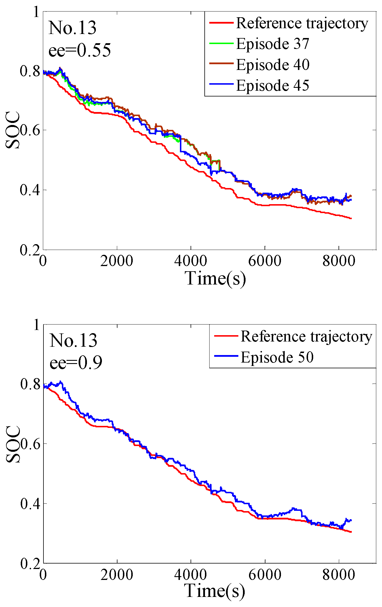
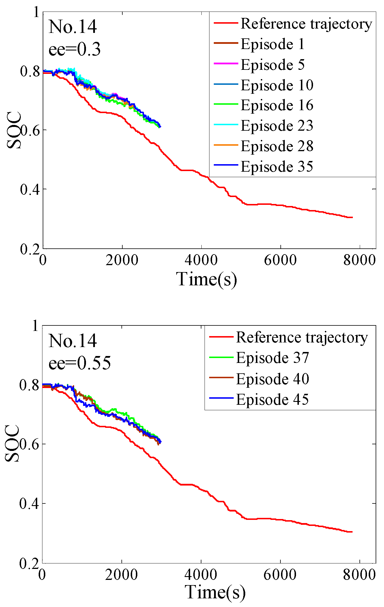
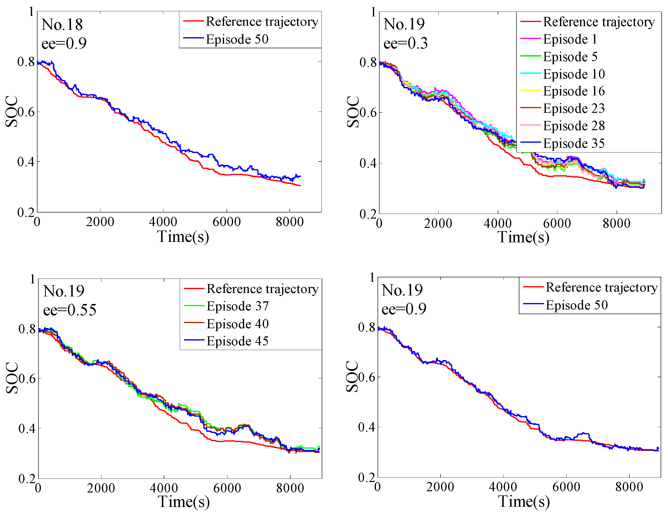
4.2. The Off-Line Training

To train the Q-table of the QL-PMP, the combined driving cycles from No.13 to No.19 in Figure 8 are deployed. The complete training process is shown in Figure 12, Figure 13, Figure 14, Figure 15, Figure 16 and Figure 17. The left figures denote the training results of the training episodes from 1 to 35, with the greedy factor of 0.3, the middle figures denote the training results of the training episodes from 36 to 45, with the greedy factor of 0.55, and the right figures denote the training results of the training episodes from 46 to 50, with the greedy factor of 0.9. The greedy factor 0.3 means that the QL-PMP tends to explore a new action to maximize the reward. The greedy factor 0.55 means that the QL-PMP tends to balance the chance between the exploration and the best action. The greedy factor 0.9 means that the QL-PMP tends to use the best action to realize the optimal control whilst providing a chance to find a better action.

As shown in Figure 12, for the training results of the combined driving cycle 13, the difference between the feedback SOC and the reference SOC is large when the greedy factor is 0.3, and the training fails all the time till the training reaches to episode 35. Moreover, although the feedback SOC trajectory is reasonable at the episode 35, the feedback SOC trajectory severely deviates from the reference trajectory. The QL-PMP becomes better and better with the continuous training, but is far from reliable When the greedy factor is 0.55, most of the feedback SOC trajectories can meet the requirements, but they are also far away from the reference SOC trajectory. When the greedy factor is 0.9, the feedback SOC trajectory of the episode 50 is reasonable and is close to the reference SOC trajectory. This implies that the trained Q-table is reasonable for the combined driving cycle 13.

As shown in Figure 13, for the training results of the combined driving cycle 14, the trainings are always fail when the episode is lower than 45 with the Q₁ (the trained Q-table with the combined driving cycle 13), which means that the Q₁ is not suitable for the combined driving cycle of 14, and the Q-table should be continually trained. Fortunately, the Q-table can be trained well enough through 45 trainings. It is worth noting that the failings of the feedback SOC trajectories do not mean that the Q₁ is not trained well, the failings are also attributed by the smaller greedy factor.

As shown in Figure 14, for the training results of the combined driving cycle 15, the feedback SOC trajectories are always reasonable for any greedy factor and any episode. This implies that the Q₂ (the trained Q-table with the combined driving cycle 14) is suitable for this combined driving cycle. Moreover, the feedback SOC trajectory of the episode 50 with the greedy factor of 0.9 is closer to the reference SOC trajectory than others, which shows that the Q-table becomes more and more reliability through the trainings from episode of 1 to 45.

As shown in Figure 15, for the training results of the combined driving cycle 16, the feedback SOC trajectories always fail when the greedy factor is 0.3. However, the control performance is continuously improved with the increasing of training number. Similarly, the trainings still fail despite the greedy factor being 0.55. This implies that the driving conditions are different from the above combined driving cycles. Therefore, the Q-table should be continuously trained based on Q₃ (the trained Q-Table with the combined driving cycle 15). However, when the episode reaches to 50, the feedback SOC trajectory is reasonable and close to the reference SOC trajectory, which implies that the Q-table has been trained well.

As shown in Figure 16, for the training results of the combined driving cycle 17, although the Q₄ (the, trained Q-Table with the combined driving cycle 16) has been well trained, the training fails before episode 44. This implies that the Q₄ still not be suitable for all of the driving conditions. However, the Q₅ (the trained Q-Table with the combined driving cycle 17) can be suitable for the combined driving cycle 17 through a series of training.

As shown in Figure 17, the training results of the combined driving cycle 18 and 19 have demonstrated that Q₅ is well trained. The QL-PMP can be directly applied to the on-line control.

5. The Hardware-In-Loop Simulation

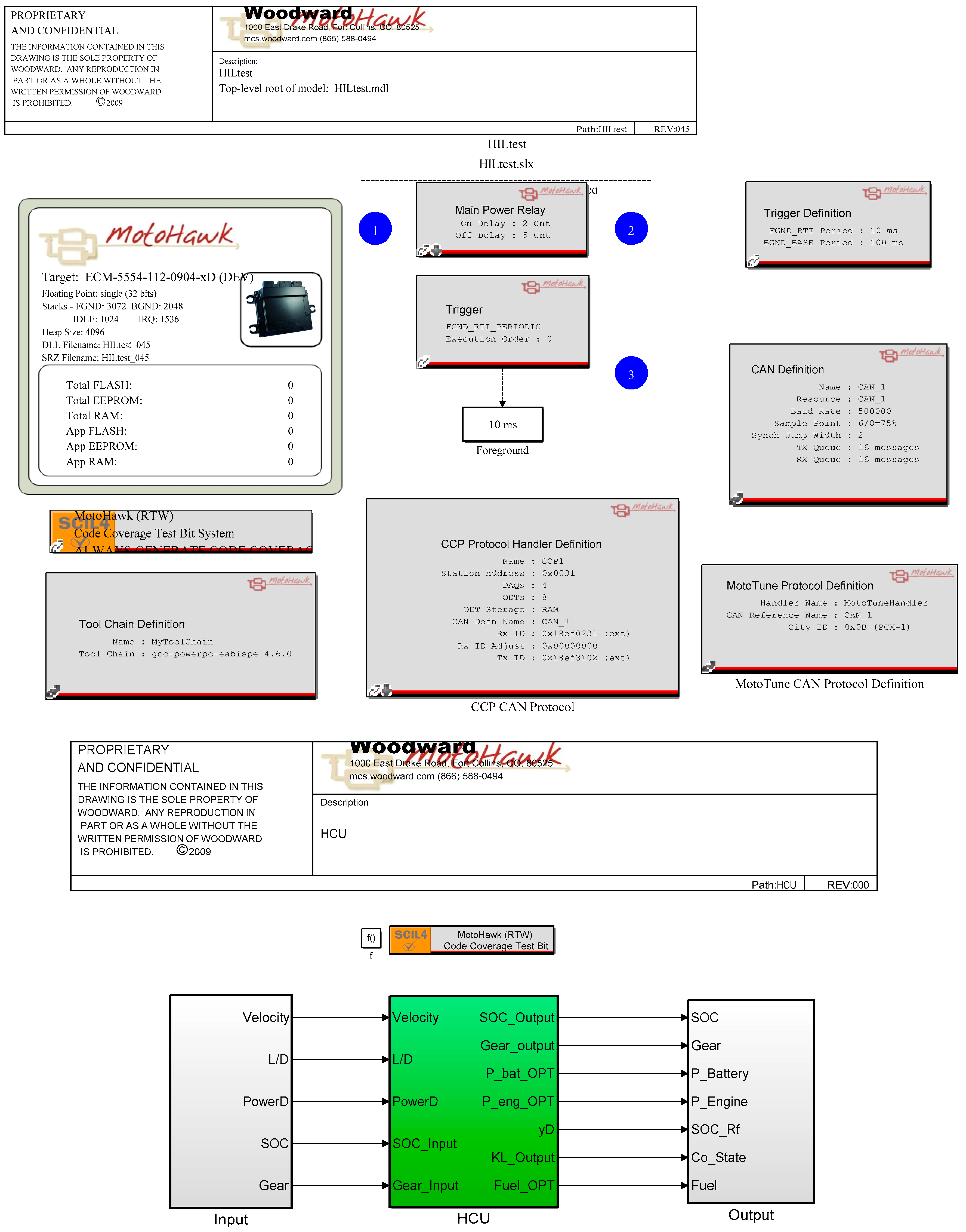
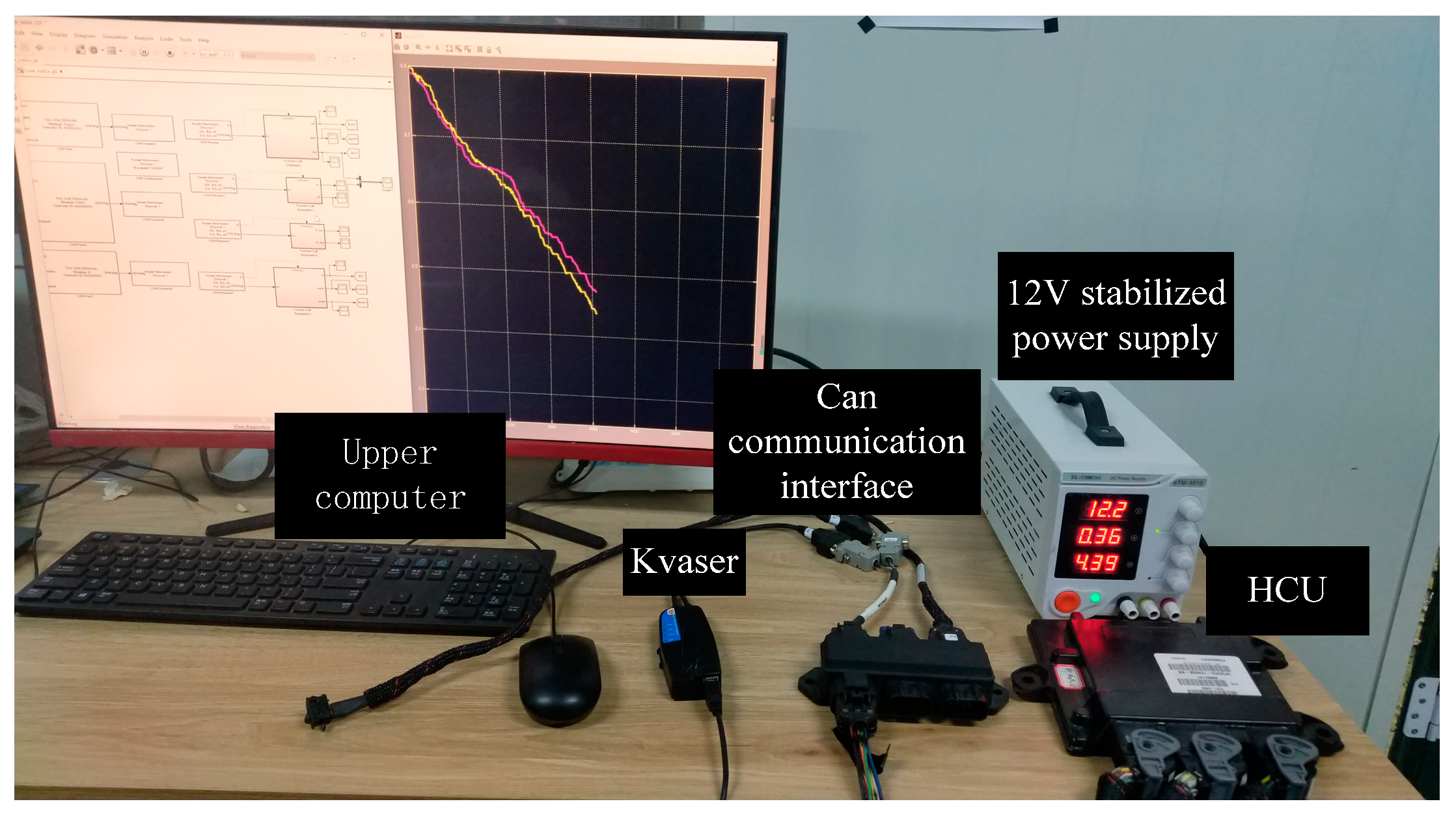
5.1. The Introduction of the HIL

To further verify the real-time and robust control performances of the EMS, a hardware-in-loop simulation (HIL) platform was also developed, based on the D2P rapid prototype control system. The D2P development platform mainly includes the MotoHawk development software and the MotoTune debugging software, where the former can bridge the gap between the control code and the MATLAB code; the latter is the debugging software for downloading and viewing the programs.

As shown in Figure 18, The Target Definition is the model selection and configuration module; the Main Power Relay is the main relay control module; the Trigger is the trigger module. In this paper, the controller type is ECM-5554-112-0904-Xd (DEV), the microprocessor is the MPC5554 of Freescale with 32-bit, and the frequency is 80 MHz. In terms of the EMS, the controlled models such as the engine, the motor and the battery are modeled as Simulink models, the algorithm of the QL-PMP will be implemented into the Hybrid Control Unit (HCU). Specifically, the QL-PMP algorithm will be firstly compiled and generated into the product-level code. Then, the code will be implemented into the HCU and the real-time communication between the Simulink models and the HCU will be built through the CAN bus.

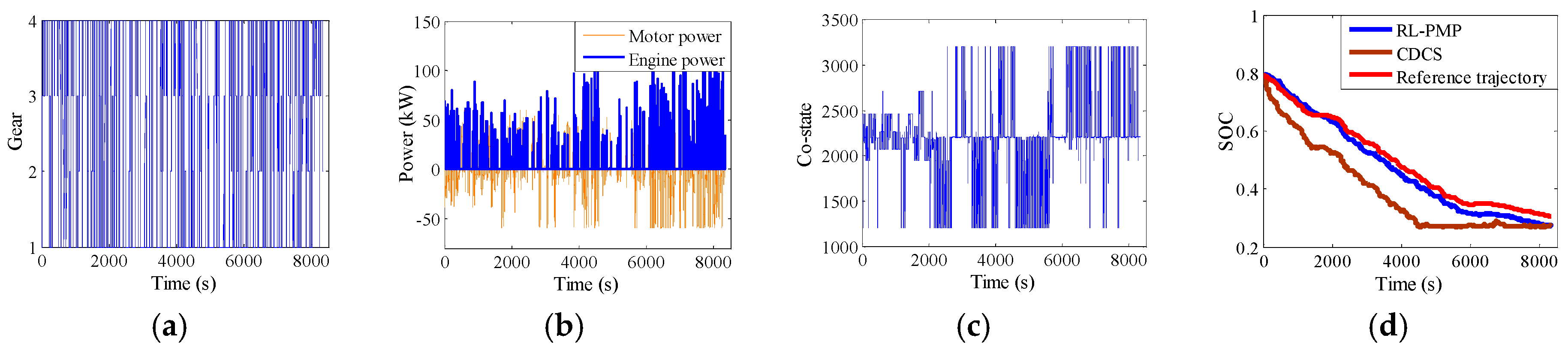
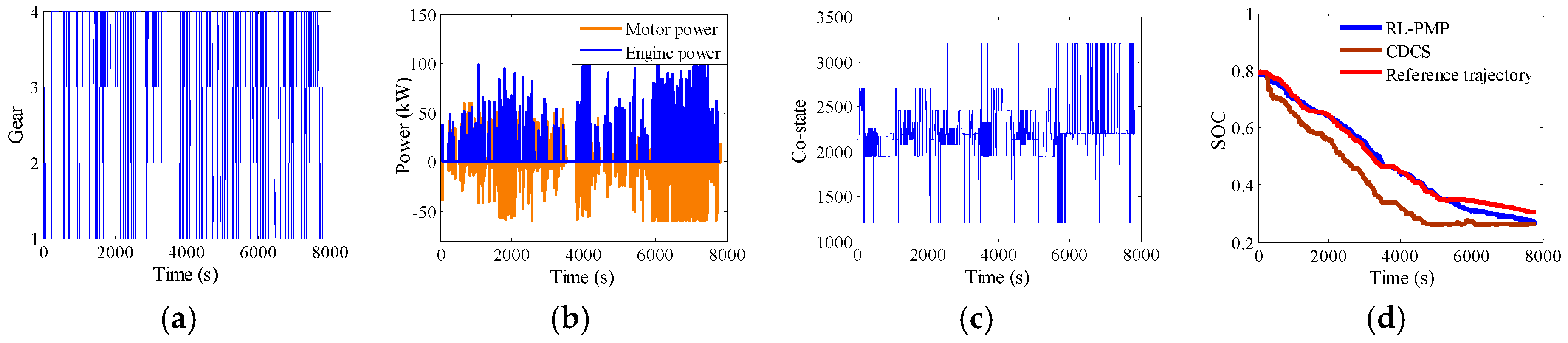
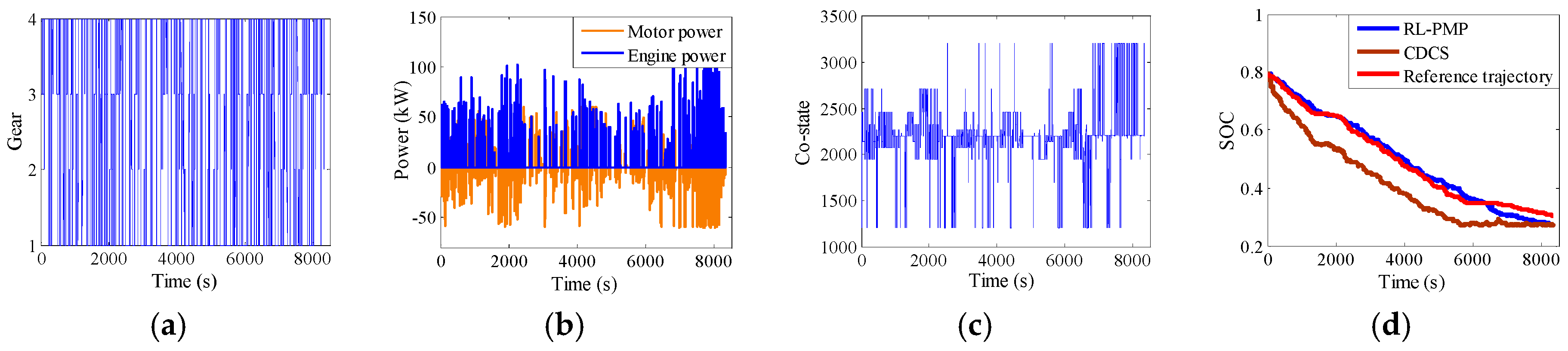
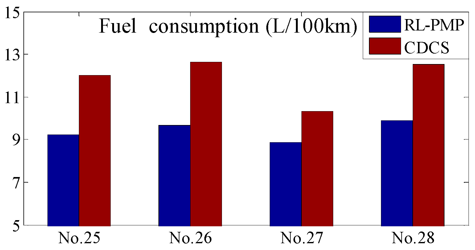
5.2. The Verification of the HIL

As shown in Figure 19, the computer is the upper computer, which sends the signals of the Simulink models and monitors the signals transmitted from the HCU, through Kvaser. As shown in Figure 20, a series of combined driving cycles from No.21 to No.24 were designed to further verify the reliability of the Q-table and evaluate the fuel economy of the QL-PMP. In addition, a rule-based energy management (named by CDCS control strategy) which is characterized by CD followed by CS control strategy was also deployed to evaluate the fuel economy of the QL-PMP.

As shown in Figure 21, Figure 22, Figure 23 and Figure 24, (a) denotes the gears, (b) denotes the powers of the motor and the engine, (c) denotes the co-state, and (d) denotes the SOC trajectories. From (a), it can be seen that the gears of the AMT tended to maintain high gear to improve the fuel economy of the PHEB. From (b), it can be seen that the engine and the motor work coordinately to provide the required power of the vehicle, meanwhile, the motor works in driving or regenerative braking modes based on the driving conditions. From (c), it can be seen that the co-states are adjusted all the time to make the feedback SOC track the reference SOC trajectory. From (d), it can be seen that the feedback SOC can track the reference SOC trajectory well, despite of any combined driving cycle. Moreover, the SOC trajectory of the CDCS control strategy is far away from the reference SOC trajectory. At the same time, the CDCS control strategy firstly works in the CD mode, and then works in the CS mode.

As shown in Figure 25, the fuel consumption of QL-PMP is significantly lower than the CDCS control strategy for any combined driving cycle, which further demonstrates the good economic performance of the QL-PMP algorithm. In specific, compared to the CDCS control strategy, the fuel economy can be improved by 23.01%, 23.57%, 14.13%, and 20.96% respectively. In a word, it can be improved by an average of 20.42%.

6. Conclusions

This paper proposes a QL-PMP based- energy management with a small state space, which can realize real-time control in dynamically stochastic traffic circumstance. The conclusions are summarized as follows:

• A self-learning energy management constituted by the QL and the PMP algorithms are proposed. The actual control variables of the throttle of the engine and the shift instruction of the AMT are exclusively solved by the PMP and the co-state in the PMP is designed as the action in the QL, which can effectively reduce the dependence of the action on the state and give a chance for the reduced state space design.
• A limited state space constituted by the difference between the feedback SOC and the reference SOC is proposed. Since the co-state is designed as the action of the QL-PMP and has weak dependence on the state, only a Q-matrix with 50 rows and 25 columns are adequate for the Q-Table. This also gives a chance for the real-time energy management control in real-world.
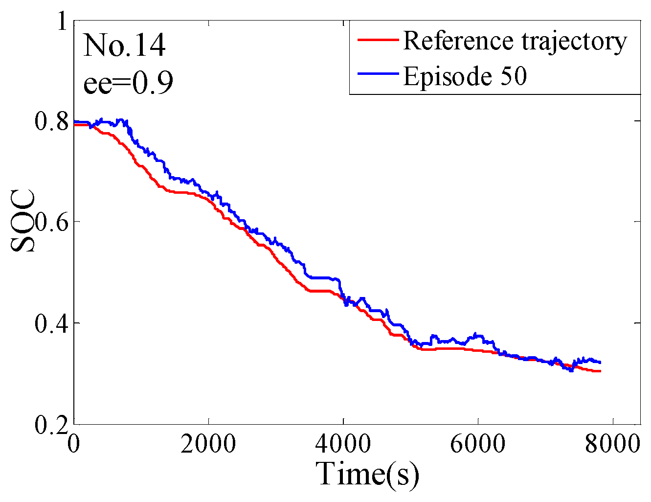
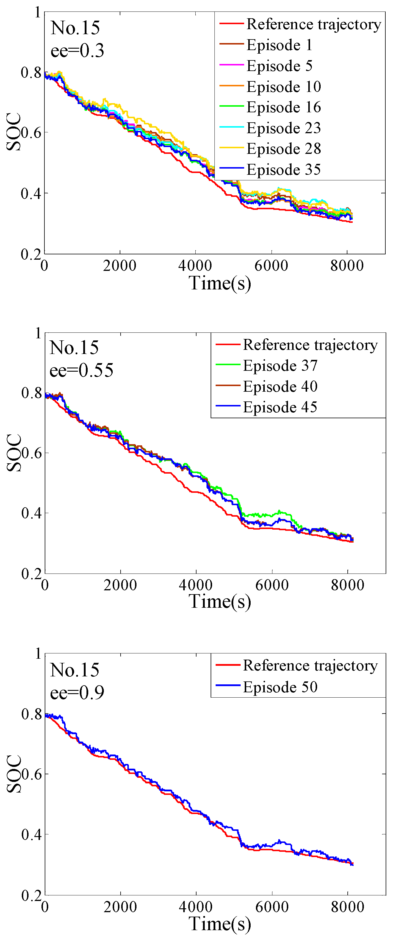
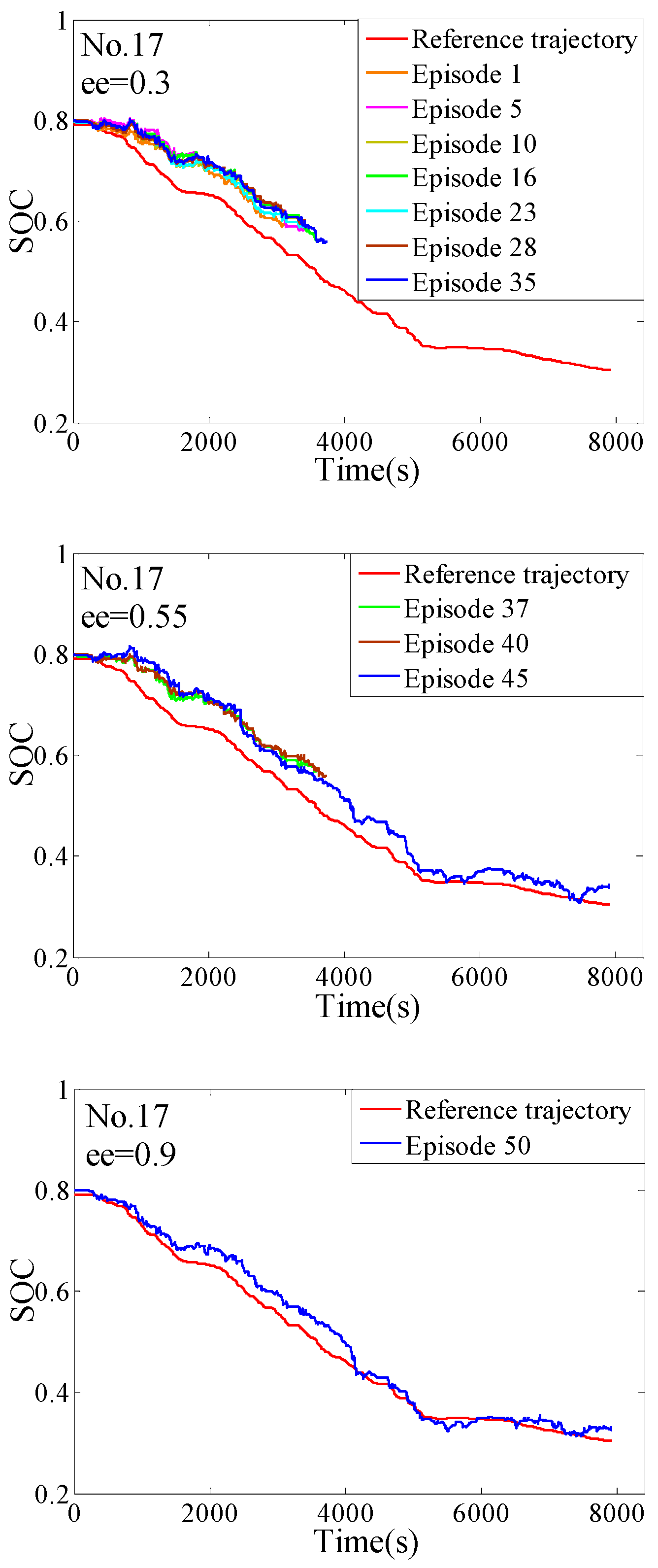
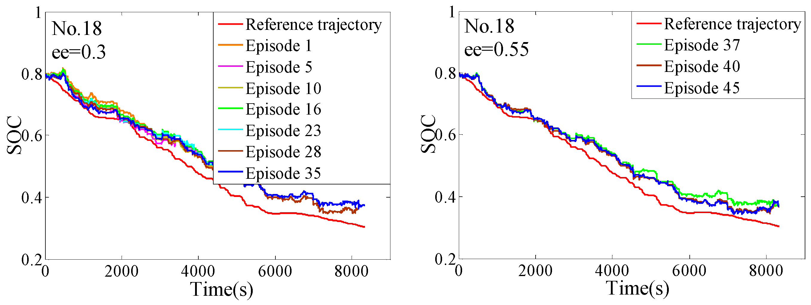
• The complete training process of the QL-PMP algorithm and the HIL verification are presented. The training process show that the QL-PMP can realize the self-learning energy management control for any combined driving cycle, where the control performance can be continuously strengthened. The verification of HIL demonstrates that the completely trained QL-PMP has high reliability, and can realize the real-time control, despite of any combined driving cycle. Moreover, the fuel economy can be improved by 20.42%, compared to CDCS control strategy.

References

1. Xie, S.; Hu, X.; Xin, Z.; Brighton, J. Pontryagin’s Minimum Principle based model predictive control of energy management for a plug-in hybrid electric bus. Appl. Energy 2019, 236, 893–905. [Google Scholar] [CrossRef]
2. Huang, Y.; Wang, H.; Khajepour, A.; Li, B.; Ji, J.; Zhao, K.; Hu, C. A review of power management strategies and component sizing methods for hybrid vehicles. Renew. Sustain. Energy Rev. 2018, 96, 132–144. [Google Scholar] [CrossRef]
3. Yan, M.; Li, M.; He, H.; Peng, J.; Sun, C. Rule-based energy management for dual-source electric buses extracted by wavelet transform. J. Clean. Prod. 2018, 189, 116–127. [Google Scholar] [CrossRef]
4. Padmarajan, B.V.; McGordon, A.; Jennings, P.A. Blended rule-based energy management for PHEV: System structure and strategy. IEEE Trans. Veh. Technol. 2016, 65, 8757–8762. [Google Scholar] [CrossRef]
5. Pi, J.M.; Bak, Y.S.; You, Y.K.; Park, D.H.; Kim, H.S. Development of route information based driving control algorithm for a range-extended electric vehicle. Int. J. Automot. Technol. 2016, 17, 1101–1111. [Google Scholar] [CrossRef]
6. Sabri, M.F.M.; Danapalasingam, K.A.; Rahmat, M.F. A review on hybrid electric vehicles architecture and energy management strategies. Renew. Sustain. Energy Rev. 2016, 53, 1433–1442. [Google Scholar] [CrossRef]
7. Zhou, Y.; Ravey, A.; Péra, M.C. A survey on driving prediction techniques for predictive energy management of plug-in hybrid electric vehicles. J. Power Source 2019, 412, 480–495. [Google Scholar] [CrossRef]
8. Tie, S.F.; Tan, C.W. A review of energy sources and energy management system in electric vehicles. Renew. Sustain. Energy Rev. 2013, 20, 82–102. [Google Scholar] [CrossRef]
9. Hou, C.; Ouyang, M.; Xu, L.; Wang, H. Approximate Pontryagin’s minimum principle applied to the energy management of plug-in hybrid electric vehicles. Appl. Energy 2014, 115, 174–189. [Google Scholar] [CrossRef]
10. Tulpule, P.; Marano, V.; Rizzoni, G. Energy management for plug-in hybrid electric vehicles using equivalent consumption minimization strategy. Int. J. Electr. Hybrid Veh. 2010, 2, 329–350. [Google Scholar] [CrossRef]
11. Li, G.; Zhang, J.; He, H. Battery SOC constraint comparison for predictive energy management of plug-in hybrid electric bus. Appl. Energy 2017, 194, 578–587. [Google Scholar] [CrossRef]
12. Onori, S.; Tribioli, L. Adaptive Pontryagin’s Minimum Principle supervisory controller design for the plug-in hybrid GM Chevrolet Volt. Appl. Energy 2015, 147, 224–234. [Google Scholar] [CrossRef]
13. Yang, C.; Du, S.; Li, L.; You, S.; Yang, Y.; Zhao, Y. Adaptive real-time optimal energy management strategy based on equivalent factors optimization for plug-in hybrid electric vehicle. Appl. Energy 2017, 203, 883–896. [Google Scholar] [CrossRef]
14. Lei, Z.; Qin, D.; Liu, Y.; Peng, Z.; Lu, L. Dynamic energy management for a novel hybrid electric system based on driving pattern recognition. Appl. Math. Model. 2017, 45, 940–954. [Google Scholar] [CrossRef]
15. Lin, X.; Wang, Y.; Bogdan, P.; Chang, N.; Pedram, M. Reinforcement learning based power management for hybrid electric vehicles. In Proceedings of the 2014 IEEE/ACM International Conference on Computer-Aided Design, San Jose, CA, USA, 3–6 November 2014; IEEE Press: Piscataway, NJ, USA, 2014; pp. 32–38. [Google Scholar]
16. Xiong, R.; Cao, J.; Yu, Q. Reinforcement learning-based real-time power management for hybrid energy storage system in the plug-in hybrid electric vehicle. Appl. Energy 2018, 211, 538–548. [Google Scholar] [CrossRef]
17. Liu, T.; Wang, B.; Yang, C. Online Markov Chain-based energy management for a hybrid tracked vehicle with speedy Q-learning. Energy 2018, 160, 544–555. [Google Scholar] [CrossRef]
18. Wu, J.; He, H.; Peng, J.; Li, Y.; Li, Z. Continuous reinforcement learning of energy management with deep Q network for a power split hybrid electric bus. Appl. Energy 2018, 222, 799–811. [Google Scholar] [CrossRef]
19. Hu, Y.; Li, W.; Xu, K.; Zahid, T.; Qin, F.; Li, C. Energy management strategy for a hybrid electric vehicle based on deep reinforcement learning. Appl. Sci. 2018, 8, 187. [Google Scholar] [CrossRef]
20. Liessner, R.; Schroer, C.; Dietermann, A.M.; Bäker, B. Deep Reinforcement Learning for Advanced Energy Management of Hybrid Electric Vehicles. ICAART 2018, 2, 61–72. [Google Scholar]
21. Qi, X.; Luo, Y.; Wu, G.; Boriboonsomsin, K.; Barth, M. Deep reinforcement learning enabled self-learning control for energy efficient driving. Transp. Res. Part C Emerg. Technol. 2019, 99, 67–81. [Google Scholar] [CrossRef]
22. Moser, I.; Chiong, R. A hooke-jeeves based memetic algorithm for solving dynamic optimisation problems. Hybrid Artif. Intell. Syst. 2009, 5572, 301–309. [Google Scholar]
23. Guo, H.; Lu, S.; Hui, H.; Bao, C.; Shangguan, J. Receding horizon control-based energy management for plug-in hybrid electric buses using a predictive model of terminal SOC constraint in consideration of stochastic vehicle mass. Energy 2019, 176, 292–308. [Google Scholar] [CrossRef]
Figure 1. The configuration of the plug-in hybrid electric bus (PHEB).
Processes 07 00672 g001
Figure 2. The BSFC map of the engine.
Processes 07 00672 g002
Figure 3. The efficiency map of the motor.
Processes 07 00672 g003
Figure 4. The simplified battery model.
Processes 07 00672 g004
Figure 5. The QL-PMP algorithm (Q-learning and Pontryagin minimum principle (PMP)) algorithm.
Processes 07 00672 g005
Figure 6. The route of the PHEB.
Processes 07 00672 g006
Figure 7. The combined driving cycles.
Processes 07 00672 g007
Figure 8. The combined driving cycles from No. 13 to No. 20.
Processes 07 00672 g008
Figure 9. The comparison between the reference SOC and the optimal SOC trajectories.
Processes 07 00672 g009
Figure 10. The relative errors between the reference and the optimal SOCs.
Processes 07 00672 g010
Figure 11. The co-state with different combined driving cycles.
Processes 07 00672 g011
Figure 12. The training process of combined driving cycle 13.
Processes 07 00672 g012aProcesses 07 00672 g012b
Figure 13. The training process of combined driving cycle 14.
Processes 07 00672 g013aProcesses 07 00672 g013b
Figure 14. The training process of combined driving cycle 15.
Processes 07 00672 g014
Figure 15. The training process of combined driving cycle 16.
Processes 07 00672 g015
Figure 16. The training process of combined driving cycle 17.
Processes 07 00672 g016
Figure 17. The training process of combined driving cycle 18 and 19.
Processes 07 00672 g017aProcesses 07 00672 g017b
Figure 18. The MotoHawk-project interface.
Processes 07 00672 g018
Figure 19. The Hardware-in-Loop (HIL) platform.
Processes 07 00672 g019
Figure 20. The combined driving cycles from No.21 to No.24.
Processes 07 00672 g020
Figure 21. The HIL results of No.21. (a) denotes the gears, (b) denotes the powers of the motor and the engine, (c) denotes the co-state, and (d) denotes the SOC trajectories.
Processes 07 00672 g021
Figure 22. The HIL results of No.22. (a) denotes the gears, (b) denotes the powers of the motor and the engine, (c) denotes the co-state, and (d) denotes the SOC trajectories.
Processes 07 00672 g022
Figure 23. The HIL results of No.23. (a) denotes the gears, (b) denotes the powers of the motor and the engine, (c) denotes the co-state, and (d) denotes the SOC trajectories.
Processes 07 00672 g023
Figure 24. The HIL results of No.24. (a) denotes the gears, (b) denotes the powers of the motor and the engine, (c) denotes the co-state, and (d) denotes the SOC trajectories.
Processes 07 00672 g024
Figure 25. The fuel consumptions of the HIL verification.
Processes 07 00672 g025