Numerical Simulation of Hydraulic Fracture Propagation in Coal Seams with Discontinuous Natural Fracture Networks

Abstract

To investigate the mechanism of hydraulic fracture propagation in coal seams with discontinuous natural fractures, an innovative finite element meshing scheme for modeling hydraulic fracturing was proposed. Hydraulic fracture propagation and interaction with discontinuous natural fracture networks in coal seams were modeled based on the cohesive element method. The hydraulic fracture network characteristics, the growth process of the secondary hydraulic fractures, the pore pressure distribution and the variation of bottomhole pressure were analyzed. The improved cohesive element method, which considers the leak-off and seepage behaviors of fracturing liquid, is capable of modeling hydraulic fracturing in naturally fractured formations. The results indicate that under high stress difference conditions, the hydraulic fracture network is spindle-shaped, and shows a multi-level branch structure. The ratio of secondary fracture total length to main fracture total length was 2.11~3.62, suggesting that the secondary fractures are an important part of the hydraulic fracture network in coal seams. In deep coal seams, the break pressure of discontinuous natural fractures mainly depends on the in-situ stress field and the direction of natural fractures. The mechanism of hydraulic fracture propagation in deep coal seams is significantly different from that in hard and tight rock layers.

1. Introduction

Coal seam gas that mainly contains methane is an economical and promising solution for the world’s energy crisis [1]. Global coalbed methane (CBM) resources are estimated to range from 84.38 Tm³ to 262.21 Tm³, of which approximately 14.44 Tm³ are recoverable [2]. China has the world’s third largest CBM reserve, totaling approximately 37 Tm³ [3,4]; however, as they are influenced by coalification, geological structure and depth, most Chinese CBM reservoirs have low permeability [5,6,7], which makes gas extraction difficult, and even leads to coal and gas outbursts [8].

Hydraulic fracturing is an efficient stimulation method that is widely used to enhance CBM production [9,10,11,12,13] by creating a new fracture network to improve the reservoirs’ permeability and by disturbing the gas in its absorbed state to promote gas desorption from coal [9,14]. Moreover, hydraulic fracturing has also been applied to destress coal seams to prevent coal and gas outbursts. Other significant applications of hydraulic fracturing include the measurement of geo-stress [15,16], stimulation in geothermal energy reservoirs [17,18], hard rock stratum breaking for ground control and mining [19,20], and underground radioactive waste disposal [21]. The application of hydraulic fracturing can be traced back to the 1860s, when liquid nitroglycerine was injected into boreholes to break rocks in the US [22]. In 1968, high-volume hydraulic fracturing was first used to extract crude oil [23]. To date, approximately 2.5 million fracturing treatments have been carried out [24]. Hydraulic fracturing for CBM extraction projects started in the US in the 1970s and in Australia in the 1990s [25].

Due to coalification and geological movement, coal seams in general include porous coal matrix, cleat systems and joint networks [26]. The cleat systems develop in each coalification stage, and are usually well-developed in low volatile bituminous coal, but poorly-developed in the lowest ranking coal or anthracite coal [27,28]. In most coal seams, discontinuous cleat systems cut across the coalbed at about 90° [28,29]. The cleat systems usually occur in two sets of roughly mutually-perpendicular cleats: face cleats and butt cleats [30,31]. Both cleats and joints constitute the main fracture network of coal seams. Natural fractures in coal seams are usually discontinuous and strength-heterogeneous due to differences in the roughness, opening, mineral fillings and extension length of fractures.

High-pressure fluid penetrates the porous coal matrix and natural fractures, resulting in a potential effect on pore pressure distribution and natural fracture propagation [32,33]. The hydraulic fracture may change its propagation direction in contact with natural fractures [34]. Therefore, hydraulic fracture propagation can be significantly affected by the pores and the discontinuous natural fracture network in coal seams [11,35,36]. Investigation of hydraulic fracture propagation and its interaction with discontinuous natural fracture (i.e., pre-existing fracture) networks is crucial to deepening the knowledge of hydraulic fracture propagation mechanisms in naturally fractured coal seams, leading to the better application of hydraulic fracturing in coal seams.

In the past decades, significant research has been focused on the mechanism of hydraulic fracture initiation and propagation [10,13,33,36,37,38,39,40,41,42,43,44,45]. Theoretically, in intact rocks or rocks with few natural macro-fractures, it is well accepted that the initial hydraulic fractures are roughly perpendicular to the direction of minimum principal stress. In this respect, geo-stress conditions have a significant effect on hydraulic fractures. The fracture initiation pressure depends on the geo-stress conditions, tensile strength, pore pressure, and porosity of coal or rock layers [26]. Several theoretical models have been put forward to predict the hydraulic fracture initiation pressure for different rock properties and pore pressure conditions [46,47,48,49].

To describe hydraulic fracture propagation in natural fracture networks, several theoretical models have been proposed based on laboratory experiments and field investigations, and can be classified into four main models [50]: pure opening mode (POM), pure shear stimulation (PSS), primary fracturing with shear stimulation leak-off (PFSSL), and mixed-mechanism stimulation (MMS). POM is a classic concept for the prediction of new and propagating hydraulic fractures that has been widely used in oil and gas extraction [10,51,52,53]. In the POM model, it is assumed that the rock crack is induced by pure tensile failure. POM is suitable for predicting hydraulic fracture propagation in reservoirs that contain only few natural fractures. PFSSL considers the leak-off behavior of fracturing liquid when the main continuous fractures propagate and meet with natural fractures [50]. Warpinski et al. [54], Palmer et al. [55], Rogers et al. [56] and Nagel et al. [57] used PFSSL to predict hydraulic stimulation in shale. MMS is based on the idea that continuous flow paths include both new and natural fractures, and that the propagating new fractures terminate in contact with natural fractures [35,58,59]. Therefore, in the MMS model, due to the natural fracture network, it is difficult to form large-scale continuous fractures, and the fracturing liquid is forced to flow through a more complex fracture network that involves both new and natural fractures. Affected by the local stress concentrations induced by the opening and slipping of surrounding fractures, hydraulic fractures not perpendicular to the minimum principal stress are forced to open at least partially [50]. Hydraulic fracture propagation and termination in MMS have been analyzed in laboratoy experiments [32,39,60,61], field investigations [62,63,64], and numerical simulations [61]. PSS is widely used in enhanced geothermal systems (EGS), and it is commonly assumed that the hydraulic liquid flow pathways mainly involve natural fractures, and that new fracture growth is usually not considered [50]. In PSS, the artificial hydraulic fracture network is formed by natural fractures connecting to each other.

Beginning with Khristianovic et al.’s work [65] in 1955, significant efforts have been applied to the development of numerical modeling techniques for hydraulic fracturing. The early studies, such as the axisymmetric penny-shaped model [66], the 2D plane strain PKN [51] and KGD [52] models, focused on the fluid–solid coupling analytical methods based on the assumption of a fracture profile. Those models solved the hydraulic fracture question by simplifying the fracture profile and the hydraulic pressure distribution. A well-known pseudo-3D model was proposed in the 1980s [67], which can model hydraulic fracture propagation for more realistic fracture profiles. After that, other analytical approaches for 2D and 3D hydraulic fractures have been proposed [10,68,69,70,71,72,73].

Furthermore, many numerical simulations using the finite element method (FEM), the boundary element method (BEM), the extended finite element method (XFEM), the cohesive element method and the discrete element method (DEM), have been performed to study hydraulic fracturing. To model hydraulic fracture propagation, the numerical governing equations should include: (1) the non-linear partial differential equations that describe the relationship between the fluid flow rate in fractures, the fracture opening width and the fluid pressure gradient; (2) the fracture initiation and propagation criteria; (3) the leak-off equations that define the diffusion process of the fracturing liquid from fractures in the coal or rock matrix [74]; and (4) seepage equations that describe the fluid seepage process in the coal or rock matrix and the variations of porosity and pore pressure. Wang et al. [75] proposed a numerical method combining FEM and a meshfree method to investigate crack propagation driven by hydraulic pressure. Yoon et al. [34,76,77,78,79] implemented and developed the fluid flow and seismicity algorithms using particle flow code 2D (PFC2D) software to model the hydraulic fracturing process in a natural pre-existing fracture network. Those algorithms allow higher permeability parameters to natural fractures that are represented by a smooth joint contact set in the PFC2D software. In addition, the PFC2D software was also adopted to simulate hydraulic fracturing by Al-Busaidi et al. [80], Shimizu [81] and Wang et al. [36,82]. Zhao et al. [83] investigated the effects of different types of natural fractures on hydraulic fractures in rock using the UDEC software. Based on the maximum tensile strain criterion, Huang [84] studied hydraulic fracture propagation and coalescence in coal seams using the RFPA software. Chen [74] modeled a single 2D hydraulic fracture using the cohesive element method and compared the numerical simulation results with analytical results, demonstrating that the cohesive element method is highly accurate when modeling hydraulic fracturing. Dahi Taleghani et al. [33] improved a traction–separation law for cohesive zone model to simulate hydraulic fracture propagation in naturally fractured formations. Zhao et al. [85] analyzed 3D hydraulic fracture propagation in coal, also using the cohesive element method.

Compared to other analytical methods and numerical simulation methods for modeling hydraulic fracturing, the cohesive element method has several advantages. (1) The cohesive element method adopts a non-linear damage zone to represent the local stress field around the crack tip, and avoids stress singularity in the crack tip, therefore providing good convergence for the fracture process numerical simulation; (2) The hydraulic fracture propagation process can be regarded as a dynamic moving process for fracture surfaces driven by fracture liquid as the propagation path is unknown in advance. Using the cohesive element method, the previously-unknown hydraulic fracture path can be dynamically calculated as a natural solution [74]; (3) The cohesive element method models microstructural damage mechanisms well (hydraulic fracture initiation, propagation, branching and coalescence with other fractures); (4) The cohesive element method can consider the leak-off behavior of fracturing liquid.

These above studies developed the simulation methods and algorithms of hydraulic fracture propagation. However, they mainly focused on hydraulic fracturing in intact rock or in continuous pre-existing joint networks. To date, hydraulic fracture propagation and interaction with the discontinuous fracture network in coal seams is still unclear.

This study proposes a hydraulic fracture propagation simulation method using the ABAQUS Software for discontinuous natural fracture networks and a preliminary analysis of hydraulic fracture morphology in coal seams. An innovative finite element meshing scheme was used to model hydraulic fracturing based on the cohesive element method, featuring global cohesive element embedding and global pore pressure node sharing techniques. A simulation methodology including leak-off and seepage effects was developed. The hydraulic fracture network characteristics, the growth mechanism of secondary hydraulic fractures, the pore pressure distribution in coal seams, and the variation of fracturing liquid pressure were investigated. Overall, this study aims to deepen the understanding of the mechanism of hydraulic fracture propagation in coal seams.

2. Simulation Methodology for Hydraulic Fracturing in Discontinuous Natural Fracture Networks

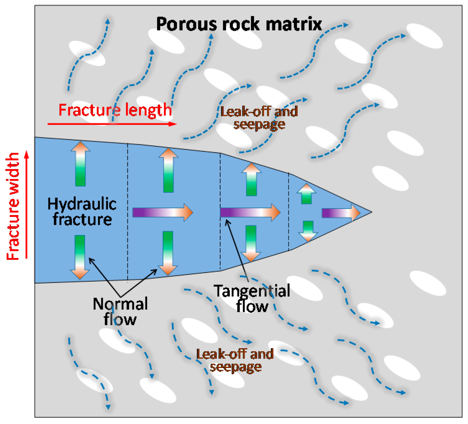
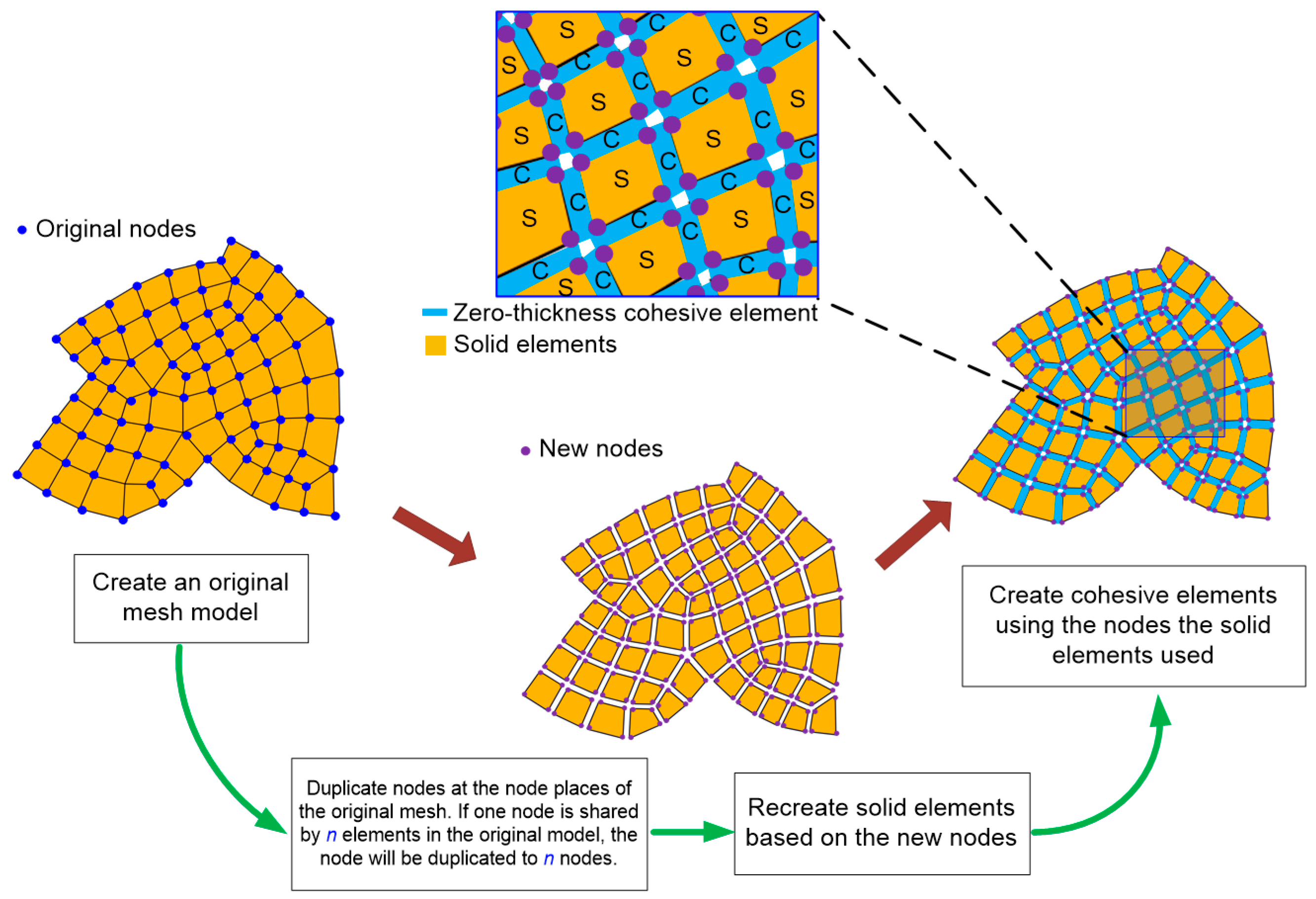
2.1. Concept and Methodology of the Hydraulic Fracturing Simulation Using the Cohesive Element Method

The cohesive element method is based on damage mechanics and the cohesive zone model (CZM). By embedding zero-thickness cohesive elements into a mesh, dynamic and unrestricted fracture propagation (especially crack branching, coalescence and swerve) can be modeled. Figure 1 illustrates the process of generating zero-thickness cohesive elements into a solid element mesh. This algorithm was coded with the Python programing language and implemented as an ABAQUS plugin to generate cohesive elements. By executing the plugin, cohesive elements are generated at every solid element interface. Therefore, the final model consists of solid elements and cohesive elements. The solid element and its neighboring cohesive element are connected by their sharing two common nodes, and the two adjacent cohesive elements connect to each other by sharing one node, as shown in Figure 1. Under internal/external traction loads, cohesive elements experience loading, damage, stiffness degradation and cracking. Crack initiation and propagation are represented by the damage and failure of cohesive elements. The coal/rock micro-elastic–plastic deformation and seepage behaviors are dominated by solid elements.

In this study, the cohesive pore pressure element (CPPE), a special type of cohesive element, was used to simulate hydraulic fracture propagation and leak-off behavior from hydraulic fractures to the porous coal matrix. As illustrated in Figure 2a, a 2D zero-thickness CPPE has six nodes and two integration points. The connection of nodes 1 and 2 forms the bottom face of a cohesive element, and nodes 3 and 4 form the top face. The relative displacements between the top and bottom faces (both in 1-direction and 2-direction) represent crack opening and slipping. Therefore, Nodes 1 to 4 are used to calculate the relationship between tractions and separations.

Nodes 5 and 6 are the pore pressure nodes, to calculate the fracturing liquid flow from one CPPE to the next CPPE (tangential flow) and leak-off from cohesive elements to solid elements (normal flow). The CPPEs are zero-thick, so the pore pressure nodes of the discrete adjacent CPPEs occupy the same coordinates after generating the discrete CPPEs in a mesh, as shown in Figure 2a (pore pressure nodes p1, p2, p3, p4 have the same coordinates P (x, y)). The fracturing liquid flow and transmission need to go through the pore pressure nodes. All the adjacent CPPEs need to share one common pore pressure node to connect to each other and to allow the fracturing liquid to flow in the fracture from one CPPE to the next. Therefore, after creating the discrete CPPEs, the pore pressure nodes at the same coordinates were merged, as shown in Figure 2b.

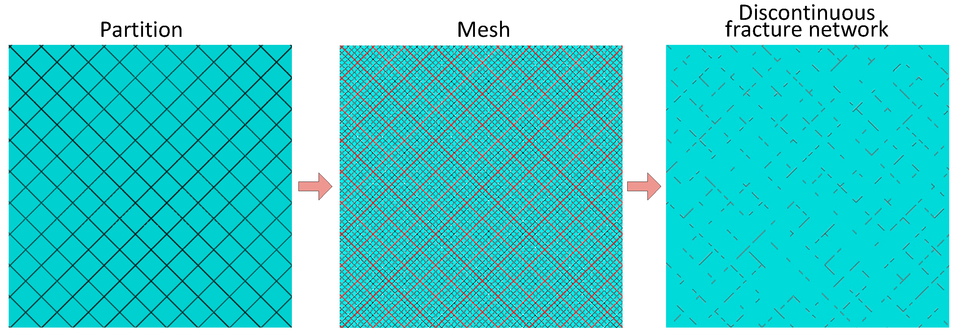
2.2. Discontinuous Natural Fracture Networks

As discussed in the introduction, natural fractures in coal seams usually have obvious directionality, thus coal seams are divided into regular hexahedral masses by the discontinuous natural fracture network. In fact, the fracture direction varies widely. This study assumed that the angle between the two sets of natural fractures was 90°, and its angle bisector was parallel to the maximum principal stress, as shown in Figure 3. The discontinuous fracture network was created as follows:

(1)

A 2D plane model was created, then this plane was partitioned by two sets of lines that are orthogonal to each other.

(2)

This plane was meshed to generate solid elements.

(3)

CPPEs were embedded in this mesh model and numbered. The serial numbers of the CPPEs that were on the two sets of partition lines into set A were picked.

(4)

A certain proportion of elements from set A was randomly selected. By assigning very low mechanical properties, these selected elements were used to represent the discontinuous fractures. The above process for the creation of a discontinuous fracture network was executed using a Python script program in ABAQUS.

3. Seepage and Hydraulic Fracture Equations

3.1. Seepage–Stress Coupling Equation for the Coal Matrix

Coal matrix is a typical porous medium that contains solid coal materials, gas-filled pores, and fracturing leak-off liquid that permeates the coal matrix during fracturing. In the seepage–stress coupling analysis, the effective stress principle was used, given by [86]:

$$\overline{\sigma }=\sigma -\chi u_{w}I$$

(1)

where $\overline{\sigma }$ is the effective stress matrix at a point, Pa; $\sigma$ is the total stress matrix, Pa; $\chi$ is the Biot coefficient; $u_w$ is the pore pressure, Pa; I is a unit matrix.

The porosity of the coal matrix, n, is defined as:

$$n=\frac{d{V}_v}{dV}$$

(2)

where $d{V}_v$ is the void volume, m³; and $dV$ is the total volume in the current configuration, m³.

The void ratio e is defined as:

$$e=\frac{d{V}_v}{dV-d{V}_v}=\frac{n}{1-n}$$

(3)

Saturation, s, is the ratio of the total free seepage volume of liquid and gas, $d{V}_w$, to the void volume, and is defined as:

$$s=\frac{d{V}_w}{d{V}_v}$$

(4)

3.1.1. Discretized Equilibrium Equation

Based on the virtual work principle, the stress equilibrium equation [87] in the current configuration can be expressed as:

$${\displaystyle {\int }_V\overline{\sigma }}:\delta \epsilon dV={\displaystyle {\int }_{S}t}\cdot \delta vdS+{\displaystyle {\int }_{V}f}\cdot \delta vdV+{\displaystyle {\int }_{V}sn{\rho }_{w}g}\cdot \delta vdV$$

(5)

where $\delta v$ is the virtual velocity field, m/s; $\delta \epsilon$ is the virtual rate of deformation tensor, s⁻¹; t is the surface traction tensor, Pa; f is the body force except the seepage liquid weight, N/m³; ${\rho }_w$ is the density of the seepage liquid, kg/m³; g is the gravity acceleration, m/s²; V is the integration domains of volume, m³; S is the integration domains of area, m². Note that the last term in Equation (5) is the weight of the seepage liquid.

In finite element analysis, the equilibrium equation is discretized into a set of equations with interpolation functions. The virtual velocity field and the virtual rate of deformation are interpolated as:

$$\{\begin{array}{l}\delta v=N^N\delta v^N\\ \delta \epsilon =\mathrm{sym}\left(\frac{\partial \delta N^N}{\partial x}\right)\delta v^N\end{array}$$

(6)

where $N^N$ is the matrix of interpolation functions defined with respect to the material coordinates; and x is the unit coordinate vector, m.

By substituting Equation (6) into Equation (5), the virtual work equation is discretized as

$$\delta v^N{\displaystyle {\int }_V{\beta }^N:\overline{\sigma }}dV=\delta v^N({\displaystyle {\int }_S{N}^N\cdot t}dS+{\displaystyle {\int }_V{N}^N\cdot f}dV+{\displaystyle {\int }_{V}sn{\rho }_w{N}^N\cdot g}dV)$$

(7)

Note that the term ${\displaystyle {\int }_V{\beta }^N:\overline{\sigma }}dV$ is the internal force array, $I^N$, and ${\displaystyle {\int }_S{N}^N\cdot t}dS+{\displaystyle {\int }_V{N}^N\cdot f}dV+{\displaystyle {\int }_{V}sn{\rho }_w{N}^N\cdot g}dV$ is the external force array, $P^N$. Therefore, the equilibrium Equation (7) can be expressed as:

$$I^N-P^N=0$$

(8)

3.1.2. Continuity Equation of Seepage

The porous coal matrix can be modeled approximately by attaching the solid element mesh to the solid materials. Thus, the liquid flows through the mesh. The time rate of the change of liquid mass in a control volume is:

$$R=\frac{d}{dt}({\displaystyle {\int }_V{\rho }_{w}sndV})={\displaystyle {\int }_V\frac{1}{J}\frac{d}{dt}(J{\rho }_{w}sn)dV}$$

(9)

where R is the time rate of change of liquid mass in a control volume, kg/s; t is time, s; J is the rate of volume change of the porous coal matrix, defined as the ratio of volume in the current configuration, $dV$, to the volume in the reference configuration, $d{V}_0$:

$$J=\left|\frac{dV}{d{V}_0}\right|$$

(10)

The liquid mass which crosses a surface, S, and flows into the control volume per unit time is:

$$F=-{\displaystyle {\int }_S{\rho }_{w}sn(n\cdot v_w)dS}$$

(11)

where $v_w$ is the liquid seepage velocity, m/s; n is the outward normal vector to S.

Obviously, the liquid mass change per unit time, R, is equal to the liquid mass flowing into the control volume per unit time, F, that is [85,88]:

$${\displaystyle {\int }_V\frac{1}{J}\frac{d}{dt}(J{\rho }_{w}sn)dV}=-{\displaystyle {\int }_S{\rho }_{w}sn(n\cdot v_w)dS}$$

(12)

According to the divergence theorem, Equation (12) can be transformed to an equivalent weak form:

$${\displaystyle {\int }_V\delta u_w\frac{1}{J}\frac{d}{dt}(J{\rho }_{w}sn)dV}+{\displaystyle {\int }_V\delta u_w\frac{\partial }{\partial x}({\rho }_{w}sn{v}_w)dV}=0$$

(13)

Equation (13) is the continuity equation of the seepage. In this study, the seepage in the porous coal matrix obeys Darcy’s law, which is given by [89]:

$$sn{v}_w=-\frac{1}{{\rho }_{w}g}k(\frac{\partial u_{w}I}{\partial x}-{\rho }_{w}g)$$

(14)

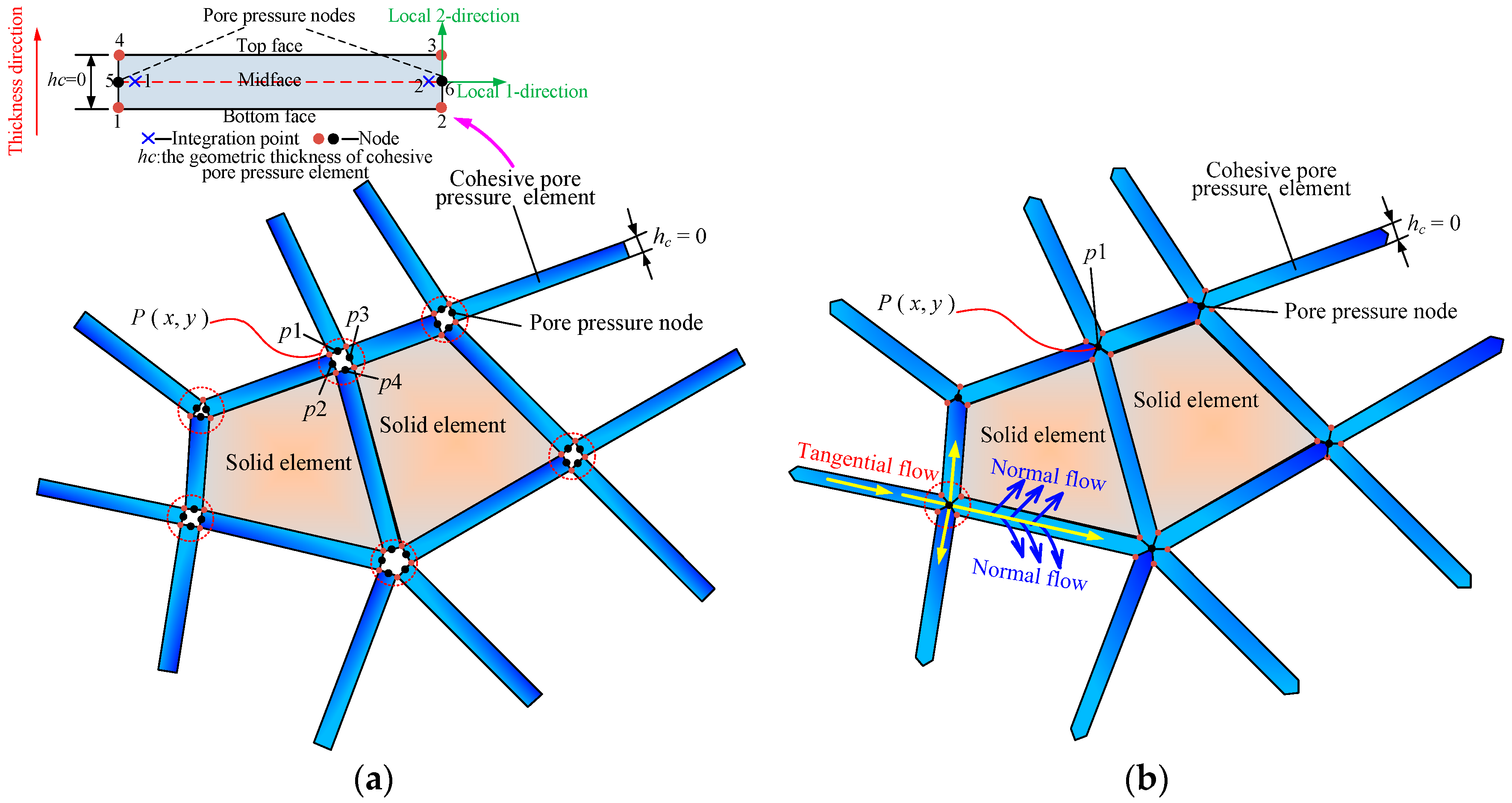
3.2. Flow Equation of the Fracturing Liquid Flow in CPPE

The constitutive response of the fracturing liquid flow in the CPPE combines tangential flow within the fracture and normal flow across the fracture, as illustrated in Figure 4. The fracturing liquid is assumed to be incompressible Newtonian. The tangential flow within the fracture is governed by [74,90]:

$$qw=-\frac{w^3}{12\mu }\nabla p_w$$

(15)

where q is the fracturing liquid flow rate per unit area, m/s; w is the opening width of the hydraulic fracture, m; μ is the viscosity of the fracturing liquid, Pa·s; $\nabla p_w$ is the pressure gradient along the CPPE, Pa/m. The term $\frac{w^3}{12\mu }$ is equivalent to the permeability or the resistance to fluid flow in the fracture.

Normal flow, representing the leak-off behavior from fractures into porous coal matrix, is defined as [74,85]:

$$\{\begin{array}{l}{q}_t=c_t(p_m-p_t)\\ q_b=c_b(p_m-p_b)\end{array}$$

(16)

where $q_t$ and $q_b$ are the leak-off flow rates in the normal direction from the mid-face into the top face and bottom face of CPPE respectively, m/s; $c_t$ and $c_b$ are the corresponding leak-off coefficients, m/Pa·s; $p_m$ is the mid-face pressure, Pa; $p_t$ and $p_b$ are the pore pressures on the top and bottom faces respectively, Pa. The leak-off coefficient can be interpreted as the permeability of the hydraulic fracture surfaces (i.e., the top and bottom faces of CPPE). According to Equation (16), the normal flow rate depends on the leak-off coefficient, and the pressure difference between the fracture (CPPE) and the porous coal matrix (solid element).

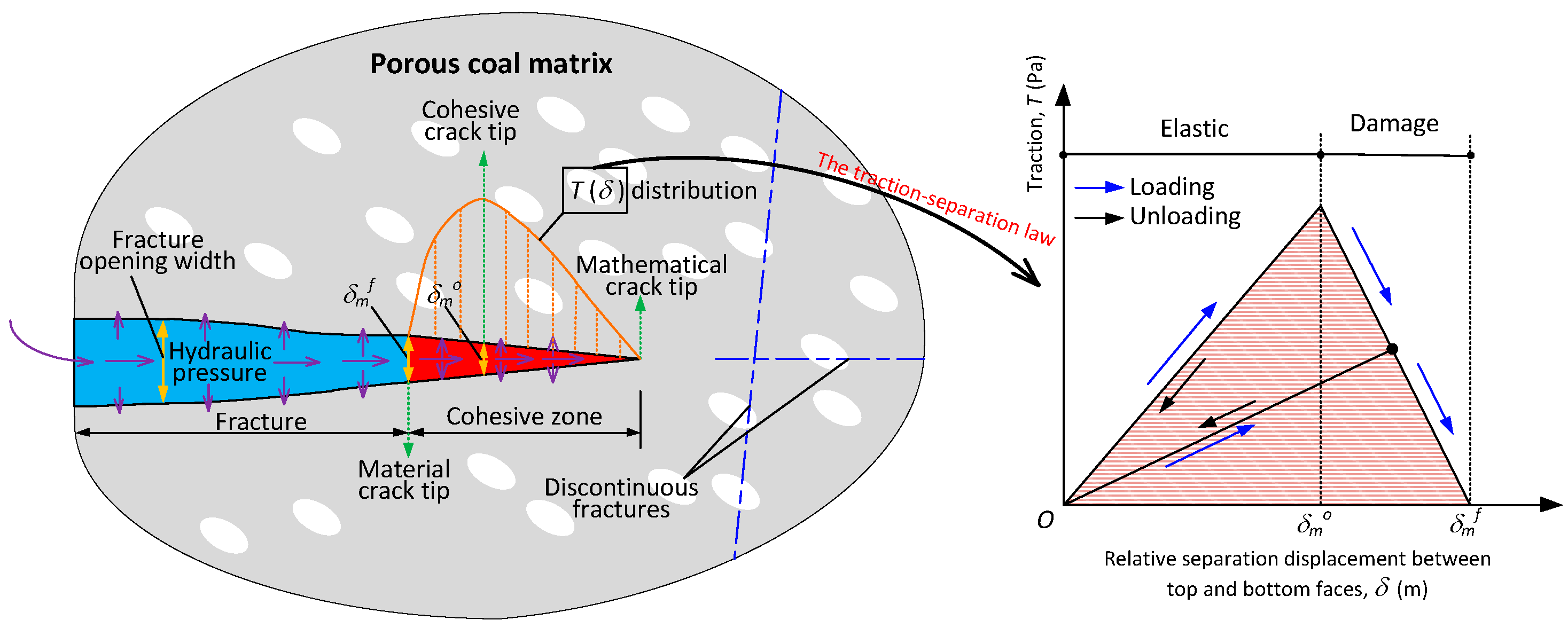
3.3. Damage Initiation and Evolution Law of Hydraulic Fractures

Crack initiation and propagation are governed by the traction–separation law. Figure 5 illustrates the fracture propagation driven by the fracturing liquid based on the cohesive element method. The traction–separation law defines the relationship between traction force, T, and the relative separation displacement between the top and bottom faces, δ. In the red cohesive zone in Figure 5, the cohesive elements are in an elastic state or in an incomplete damage state. ${\delta }_m^o$ is the critical separation displacement at the initial damage point, and ${\delta }_m^f$ is the critical displacement at the complete failure point. When $\delta \ge {\delta }_m^o$, the cohesive element starts to damage, and its stiffness decreases as T increases. When $\delta \ge {\delta }_m^f$, the stiffness of the cohesive element reduces to zero, which indicates that the fracture propagates forward. The cohesive elements in the blue fracture zone are in the complete damage state. Even if those CPPEs in the complete damage state close again from an open state, their tensile stiffness cannot recover. The concept of the crack tip was referenced from the literature [91]. The point of $\delta ={\delta }_m^f$ is the material crack tip, while the point of $\delta ={\delta }_m^o$ is the cohesive crack tip. The cohesive elements between the two crack tips are in the damaged state. The traction force, T, is the resultant force of hydraulic pressure in the cohesive element, pore pressure in the adjacent solid element, and geo-stress. Therefore, the hydraulic fracture is affected by fracturing pressure, the discontinuous natural fracture network, the seepage process in the coal matrix and geo-stress.

To model crack initiation and propagation in different materials using cohesive elements, various traction–separation models were developed. In this work, the irreversible bilinear model was used to simulate hydraulic fracture opening and closing behaviors. This model was also used by Chen [74] and Zhao et al. [85] to model hydraulic fracturing in rock. The model assumes that the mechanical response of cohesive elements satisfies a reversible linear elastic behavior prior to the initial damage point. The bearing capacity of cohesive elements decreases linearly in the damage evolution stage, and their stiffness cannot recover during unloading. The irreversible bilinear model was introduced as follows.

3.3.1. Damage Initiation

The tension component of traction force is mainly induced by hydraulic pressure, while the shear component of traction force may be caused by geo-stress differences and the local shear stress concentration around the natural fracture. Therefore, it is significant and necessary to consider the combined effects of the tension force and the shear force when modeling hydraulic fracture initiation and propagation in coal seams. Thus, a quadratic stress criterion that incorporates the tension and shear mixed modes was used to predict damage initiation occurrence. The 2D crack damage initiates when the stress state of the cohesive elements satisfies [33,85]:

$${\left(\frac{t_n}{{\sigma }_t}\right)}^2+{\left(\frac{t_s}{{\sigma }_s}\right)}^2=1$$

(17)

where ${\sigma }_t$ and ${\sigma }_s$ are tensile and shear strength, respectively, Pa; $t_n$ and $t_s$ represents normal traction (along the local 2-direction in Figure 2a) and shear traction (along the local 1-direction in Figure 2a), respectively, Pa.

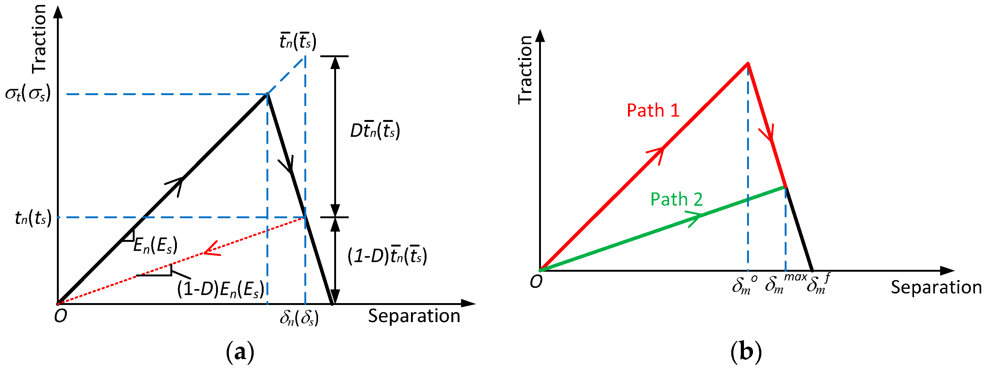
3.3.2. Damage Evolution

A scalar damage variable, D, is defined to represent the overall damage degree in one cohesive element. D evolves from 0 to 1 monotonically upon further loading after damage initiation. Stress components are affected by the damage according to [92]:

$$\{\begin{array}{l}{t}_n=(1-D){\overline{t}}_n,\mathrm{tensile}\mathrm{state}\\ t_n={\overline{t}}_n,\mathrm{compressive}\mathrm{state}\\ t_s=(1-D){\overline{t}}_s\end{array}$$

(18)

where ${\overline{t}}_n$ and ${\overline{t}}_s$ are stress components predicted by the linear elastic law at the current separation displacement, Pa, as shown in Figure 6a. Note that in Equation (18), the tensile stiffness of cohesive elements is degraded at the damage stage, whereas the compressive stiffness is unchanged.

For the linear damage softening evolution, D is expressed as [33,85,93]:

$$D=\frac{{\delta }_m^f({\delta }_m^{\max }-{\delta }_m^o)}{{\delta }_m^{\max }({\delta }_m^f-{\delta }_m^o)}$$

(19)

where ${\delta }_m^{\max }$ is the maximum value of the relative separation displacement recorded during the loading history, m. As illustrated in Figure 6b, the loading history is the loading along the red path (path 1) or reloading via the green path (path 2). Both ${\delta }_m^o$ and ${\delta }_m^f$ consist of tensile and shear separation displacement components.

The power law criterion of fracture energy is widely used to predict the complete damage state, given by [94]:

$${\left(\frac{G_I}{G_{IC}}\right)}^{\alpha }+{\left(\frac{G_{II}}{G_{IIC}}\right)}^{\alpha }=1$$

(20)

where $G_I$ and $G_{II}$ are energy components of tension and shear respectively, Pa·m; $G_{IC}$ and $G_{IIC}$ are I-mode and II-mode fracture energies respectively, Pa·m. When $G_I$ and $G_{II}$ satisfy Equation (20), the damage variable D reaches 1.

Note that the stress state and the corresponding displacement at the initial damage point is determined by Equation (17) and the relationship between T and δ; therefore, the separation displacement components at the initial damage point of each cohesive element can be different. ${\delta }_m^{\max }$ is a function of $G_I$ and $G_{II}$. ${\delta }_m^f$ is calculated using the fracture energies $G_{IC}$ and $G_{IIC}$. If ${\sigma }_t$, ${\sigma }_s$, $G_{IC}$ and $G_{IIC}$ are given, for a displacement state ${\delta }_m^{\max }$, its corresponding damage variable D can be calculated using Equation (19), and then the stress components are updated by substituting D into Equation (18). Hydraulic fracture propagation is simulated using this damage law.

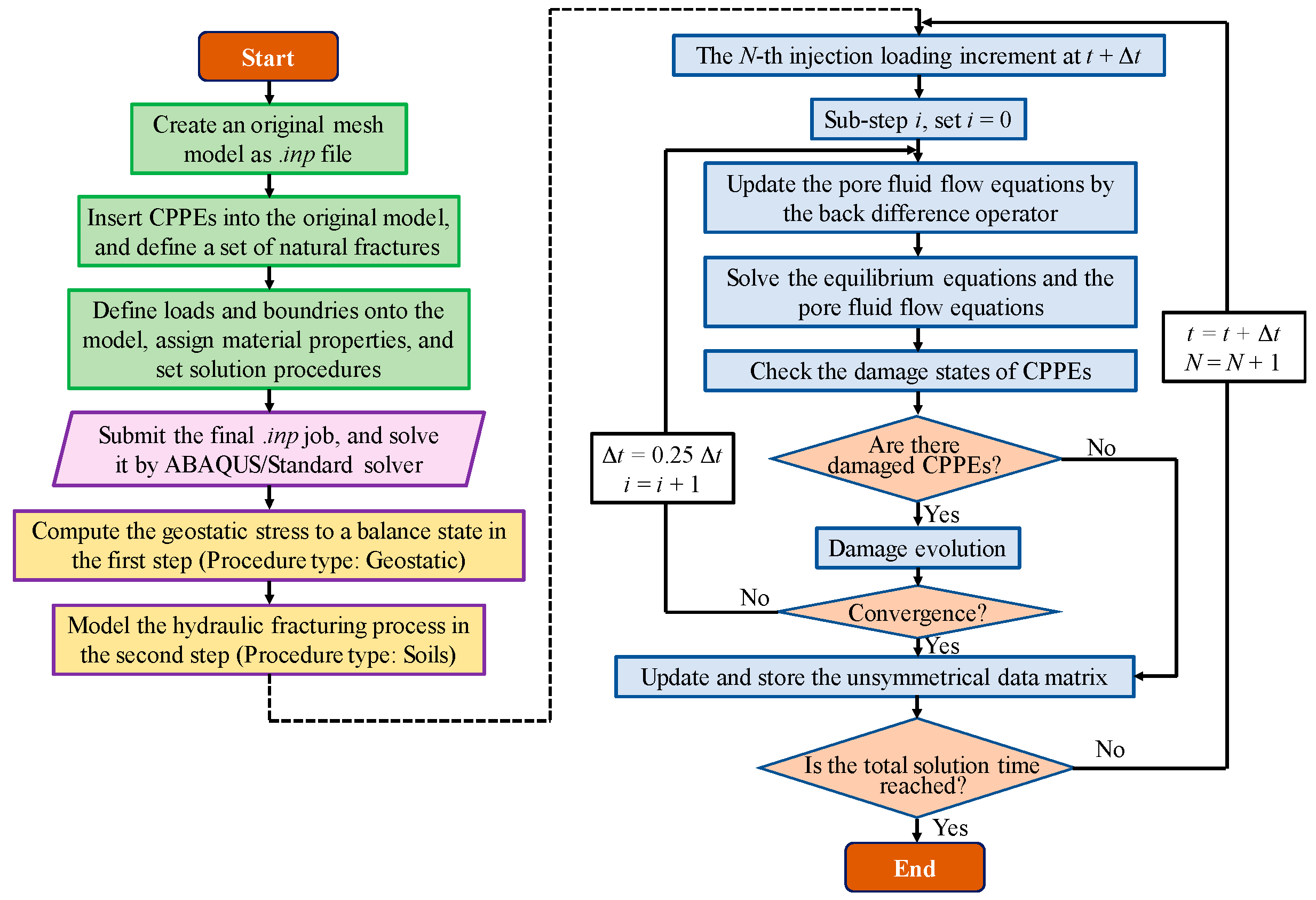
4. Numerical Simulation Procedure

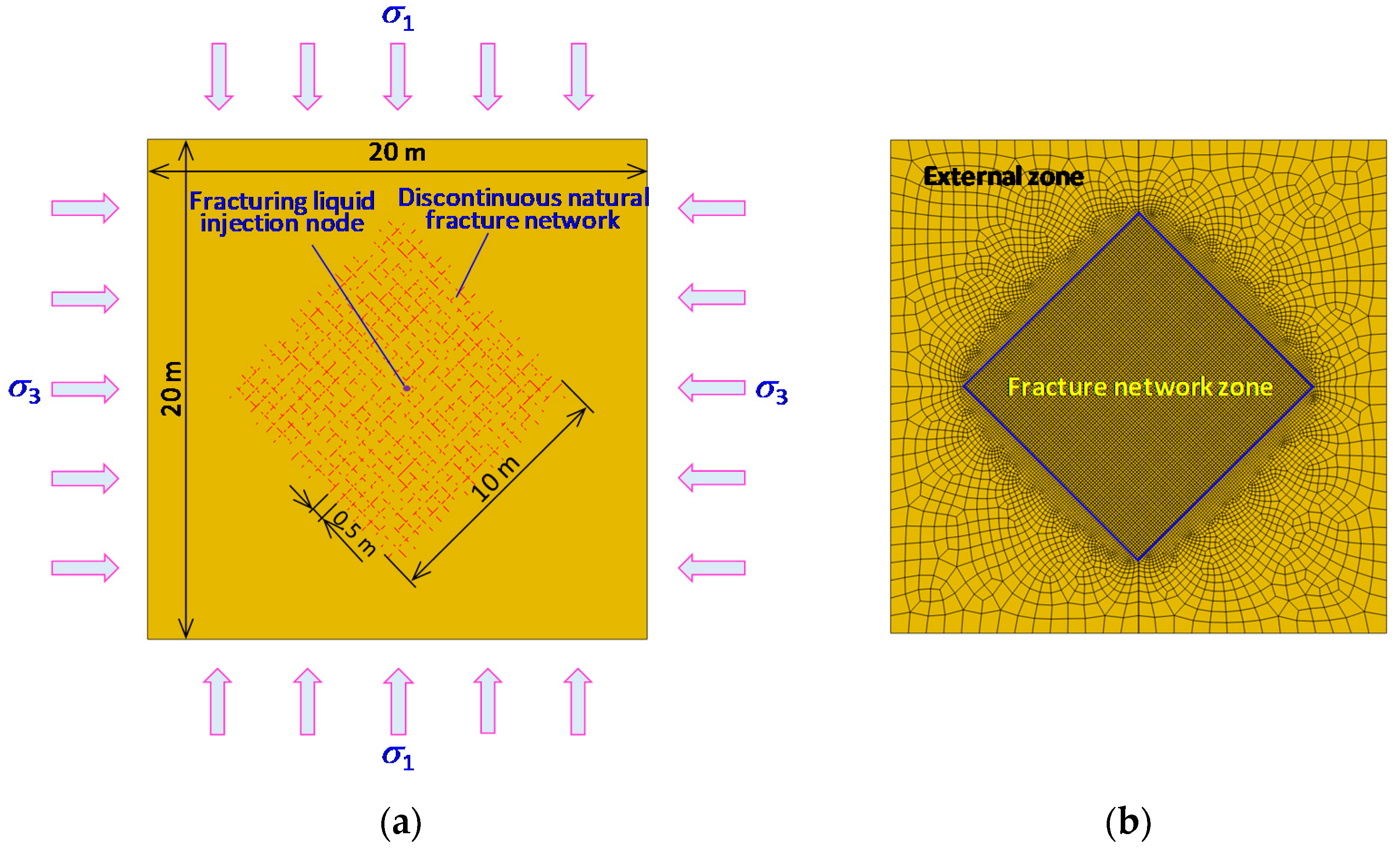
4.1. The Mesh Model of Coal Seams with Discontinuous Natural Fracture Networks

By setting the out-of-plane dimension as 3 m, the 2D numerical coal seam model was equivalent to a 3D model with a thickness of 3 m. As shown in Figure 7, the model is a square with the dimensions 400 m². To avoid the boundary effect, the discontinuous natural fracture network zone is at the center of the model, with a size of 10 m × 10 m. The two fracture sets are orthotropic with each other, and their bisector is parallel to the direction of the principle stress. The fracture spacing was set to 0.5 m. The fracture network zone’s mesh consists of 10,000 pore fluid/stress elements (the solid elements) of size 0.1 m and 20,200 CPPEs. The external zone’s mesh consists of 5612 pore fluid/stress elements of size 0.1 m to 0.6 m. The pore fluid/stress elements used were four-node plane strain quadrilateral, bilinear displacement, bilinear pore pressure elements (called CPE4P in ABAQUS).

4.2. Mechanical Properties of the Coal Matrix, Discontinuous Natural Fracture and Fracturing Liquid

Many studies show that hydraulic fracturing has significant effects on the permeability, leak-off coefficient, and porosity of coal seams [85,95,96,97]. According to Xu et al. [38], the dynamic permeability k, the dynamic porosity n and the dynamic leak-off coefficient c can be calculated as follows:

$$k=k_0\exp (3C_f\Delta p)$$

(21)

$$n=n_0(1+C_f\Delta p)$$

(22)

$$c=c_0\sqrt{1+C_f\Delta p}\exp (\frac{3}{2}{C}_f\Delta p)$$

(23)

Here, $k_0$ is the initial permeability, m/s; $\Delta p$ is the pressure difference between the fracture (CPPE) and the porous coal matrix (solid element), Pa; $n_0$ is the initial porosity; $c_0$ is the initial leak-off coefficient, m/Pa·s; $C_f$ is the pore compressive coefficient; and $C_f=(n-n_0)/(n\cdot \Delta p)$, Pa⁻¹.

The user subroutine was used to model the dynamic variation of the coal seepage properties. In one numerical increment step, if $\Delta p$ is determined, n can be calculated using Equation (22), and then $C_f$ can be obtained. k and c are then calculated using Equations (21) and (23). Until this point, k, n and c were updated dynamically. In the next incremental step, these parameters were set as the updated initial values and substituted into the governing equations for the seepage to model the dynamic fracturing process.

The mechanical properties used in this numerical model are listed in

Table 1. The mechanical properties of the discontinuous fractures, coal matrix and fracturing liquid.

Object	Mechanical Parameter	Value
Coal matrix	Elastic modulus (GPa)	5
	Poisson’s ratio	0.28
	Tensile strength (MPa)	0.77
	Shear strength (cohesion) (MPa)	6.42
	Initial permeability (m/s)	5 × 10−8
	Initial porosity	0.15
	I-mode fracture energy (N/m)	29.25
	II-mode fracture energy (N/m)	35.97
	Initial leak-off coefficient (m/Pa·s)	5 × 10−14
Discontinuous natural fractures	Tensile strength (MPa)	0.005
	Shear strength (MPa)	0.04
	I-mode fracture energy (N/m)	0.19
	II-mode fracture energy (N/m)	0.23
	Initial leak-off coefficient (m/Pa·s)	5 × 10−14
Fracturing liquid	Viscosity (Pa·s)	0.005
	Density (kg/m3)	1000

. Note that the mechanical strengths of the discontinuous natural fractures are significantly weaker than those of the coal matrix.

4.3. Initial Conditions

In this study, the injection rate of the fracturing liquid via the injection node was 0.003 m³/s; the initial gas pore pressure in the coal seams was 5 MPa. To analyze the hydraulic fracture propagation and its interaction with natural fractures under different ground stress conditions, four different stress conditions were applied, as shown in

Table 2. Stress conditions.

Group	Minimum Principal Stress, σ3 (MPa)	Maximum Principal Stress, σ1 (MPa)	Stress Difference (MPa)
A	10	12.5	2.5
B	10	15	5
C	10	17.5	7.5
D	10	20	10

.

4.4. Solving Procedures, Convergence Criterion and Error Control

Figure 8 illustrates the pre-processing and the solving procedures of the ABAQUS/Standard solver. The model first calibrates geostatic stress to a balance state and then computes hydraulic fracturing. For the two steps above, the procedure types were ‘geostatic’ and ‘soils’, respectively. The module ‘soils’ in ABAQUS allows users to model hydraulic fracturing and fluid flow through porous media. In the ‘soils’ module, the transient analysis method and the direct backward difference operator were used to optimize the accuracy of the continuity equation.

The solution technique used was the full Newton method for nonlinear equilibrium equations. In pore liquid flow analysis, pore pressure, $u_w$, was selected as a field index to evaluate the accuracy of the Jacobian matrix solution. According to the ABAQUS documentation [98], most nonlinear calculations are sufficiently accurate if the error of the largest field index residual is less than 0.005. In this study, the convergence criterion was also used:

$$r_{\max }^{u_w}\le 0.005{\tilde{q}}^{u_w}$$

(24)

where $r_{\max }^{u_w}$ is the largest residual in the pore pressure balance equation, m³/s; ${\tilde{q}}^{u_w}$ is the overall time-averaged value of a typical flux for $u_w$ until this point during this step, including the current increment, m³/s.

To guarantee the accuracy of the fracture propagation when using CPPE, the cohesive element size should be smaller than the cohesive zone length $d_c$, which is determined by the material mechanical properties, and is calculated as [74]:

$$d_c=\frac{9\pi }{32}\frac{E}{(1-v^2)}\frac{G_{IC}}{{\sigma }_t^2}$$

(25)

where E is the Young’s modulus, Pa; v is the Poisson’s ratio. By substituting the parameter values from Table 1 into Equation (25), $d_c$ = 0.182 m. The cohesive element size used in this study was 0.1 m, which is significantly less than d_c. This suggests good error control for modeling hydraulic fracture propagation.

5. Results and Discussion

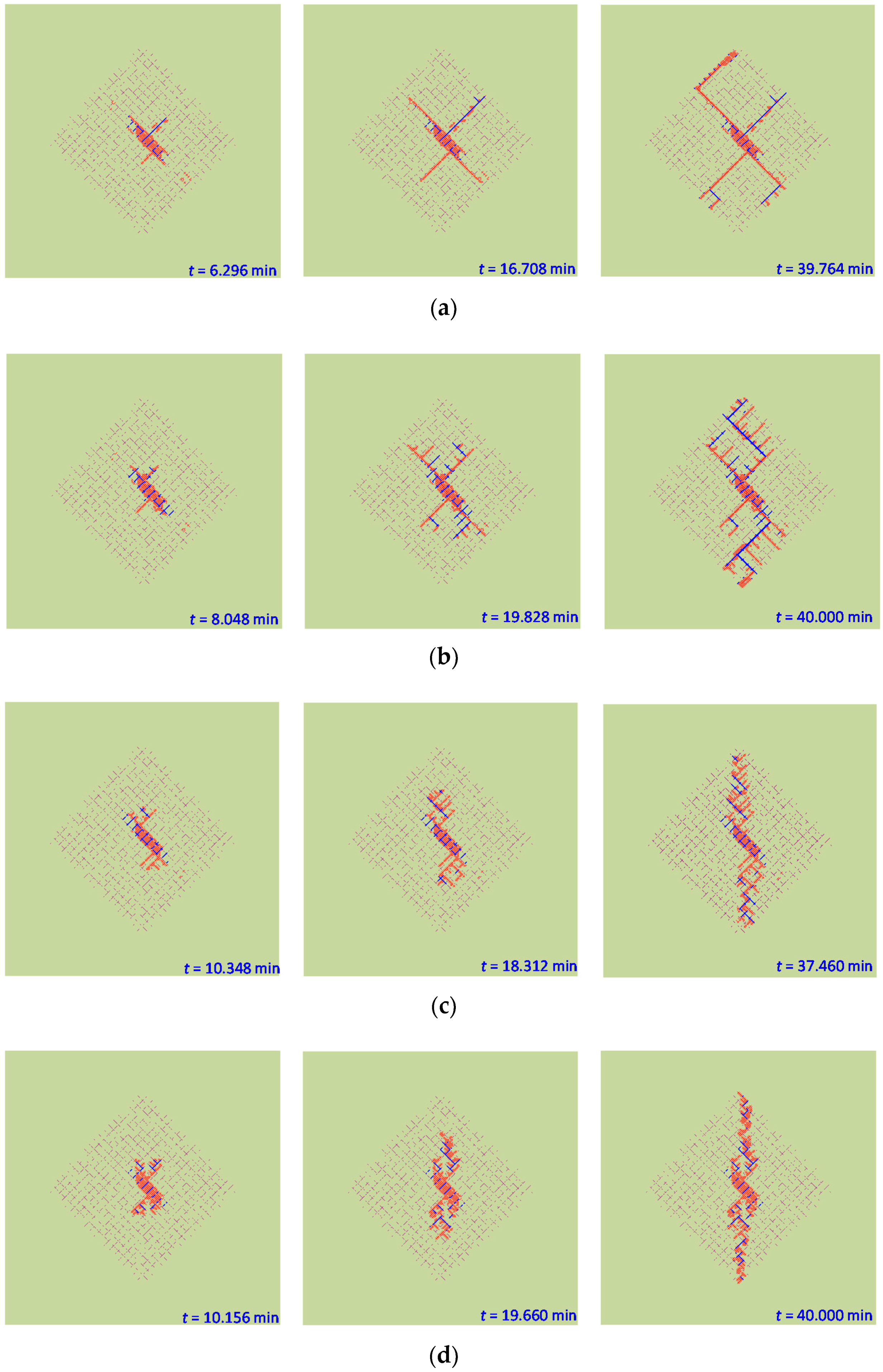
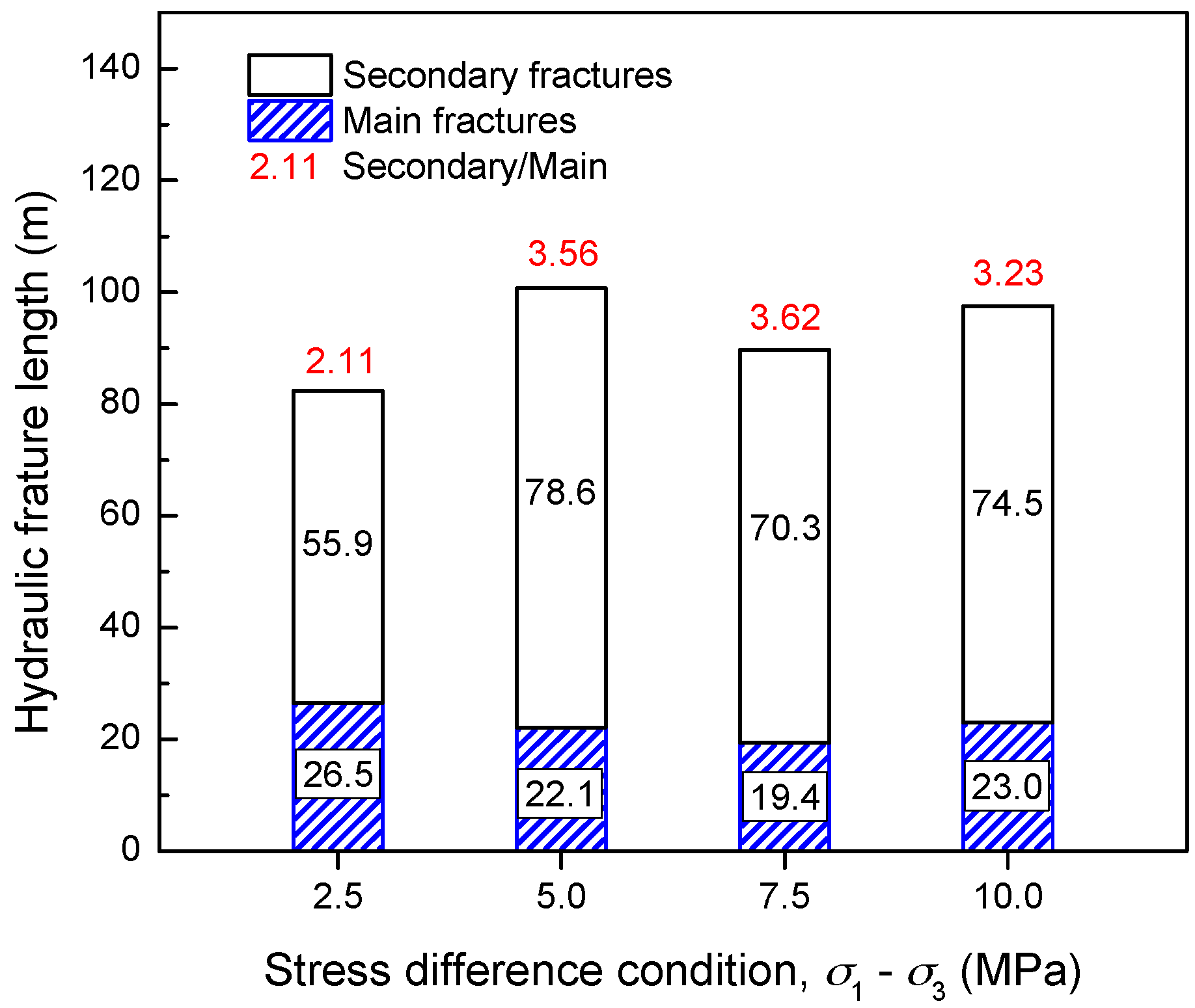
5.1. Hydraulic Fracture Network Characteristics

The CPPEs with fracturing liquid flowing were selected and marked as hydraulic fractures during the fracturing process. Figure 9 shows the hydraulic fracture network characteristics under different stress conditions. According to this figure, hydraulic fractures in coal seams are not just a single crack, but a complex fracture network. Micro-seismic monitoring in the field also confirms that hydraulic fractures in coal seams usually form a network of fracture branches using the horizontal well technique [99].

Figure 9 shows that the hydraulic fracture network has a main fracture trunk with many fracture branches. However, the main fractures are not strictly defined. Generally, this usually refers to the more prominent fractures with a relatively large opening. In hydraulic fracturing, the main fractures are the main liquid flow fracture channels. The fracture opening degree and the stiffness of the CPPEs are indicators of main hydraulic fractures. The main hydraulic fractures were identified by magnifying the hydraulic fracture opening 20 times, as shown in Figure 10.

During the initial hydraulic fracturing stage, the total fracture volume is small, thus a reticulated secondary fracture structure is created around the injection node (i.e., the injection borehole) when subject to the impact of high-pressure fracturing liquid, as shown in Figure 9. Then the total volume of fractures increases gradually, which in turn increases the fracturing liquid leak-off and weakens fluid impact. During the later stage, the secondary fractures grow from the main fracture trunk like branches.

In Figure 9, the maximum width of the hydraulic fracture network gradually narrows as the stress difference increases, indicating that the general direction of the fracture network follows ${\sigma }_1$ under high stress difference conditions. However, when ${\sigma }_1-{\sigma }_3$ = 2.5 MPa, the main hydraulic fractures propagate straight along the natural fractures. These results suggest that the general direction of hydraulic fracture networks in coal seams is jointly influenced by geo-stress differences and pre-existing natural fracture networks. When the ground stress difference is insignificant, the natural fracture network dominates the direction of the main hydraulic fractures. On the contrary, the maximum principal stress shows strong control over the general direction of the hydraulic fracture network, but the hydraulic fracture network still has many secondary fractures.

When the stress difference is 7.5 MPa or 10 MPa, the hydraulic fracture network is spindle-shaped. As the fractures propagate, the general direction of the hydraulic fracture network gradually converges to the direction of ${\sigma }_1$, and the number of secondary fractures gradually decreases. To better understand how the stress field and natural fractures affect the hydraulic fracture morphology, tests that consider the direction and discontinuous degree of the natural fractures must be carried out in the future. The improved cohesive element method used in this study is leading to continuing research on these topics.

The total lengths of hydraulic fractures under different stress conditions were counted, as illustrated in Figure 11. According to the figure, the total lengths of the hydraulic fractures were between 82.4 m (when ${\sigma }_1-{\sigma }_3$ = 2.5 MPa) and 100.7 m (when ${\sigma }_1-{\sigma }_3$ = 5 MPa). There was no obvious correlation between the total length and stress difference. In each stress condition, the total length of the secondary fractures was significantly bigger than that of the main fracture. The ratio of secondary fracture total length to that of the main fracture was between 2.11 and 3.62, which shows no obvious correlation with stress difference. The results indicate that: (1) hydraulic fracturing can create a large number of secondary fractures in coal seams; (2) stress difference has no significant effect on the total length of the hydraulic fracture and the ratio of the secondary fracture length to the main fracture length.

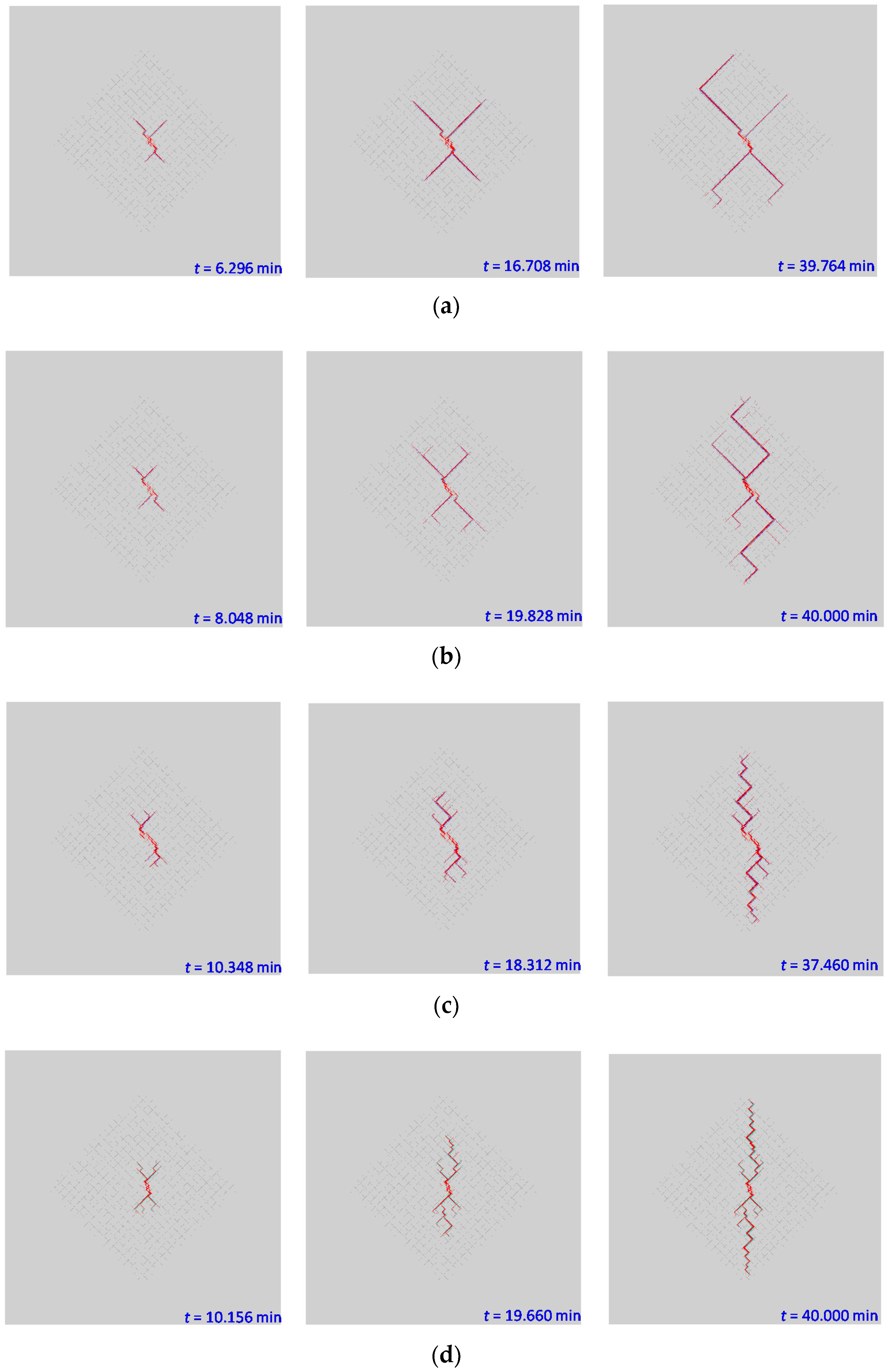
5.2. Growth Process of the Secondary Hydraulic Fractures

According to Figure 9 and Figure 10, the secondary fractures contain new fractures and natural fractures. There are two causes of secondary cracks: change to local stress fields caused by hydraulic fracture propagation and seepage in the porous coal matrix, and pre-existing low-intensity natural fractures. Figure 12 shows the growth process of secondary fractures during hydraulic fracturing when ${\sigma }_1-{\sigma }_3$ = 7.5 MPa. As the main fracture propagates, the secondary fractures gradually branch out of the main fracture trunk. At t = 8.380 min, fracture branch 1 appears. At t = 13.244 min, fracture branches 2 to 6 appear, and branch 1 grows longer due to the fracturing liquid. At t = 21.696 min, new fractures 7 to 13 appear as the main fracture propagates. Note that fractures 7, 9 and 10 grow on the secondary fractures and are considered micro-secondary fractures. The hydraulic fracture network shows a multi-level branch structure.

The main fracture in Figure 12 propagates from natural fractures to the coal matrix, and then swerve back along the natural fracture. Affected by the stress field and discontinuous natural fracture network, some secondary fractures, such as fracture branches 5, 6, 8, 12, propagate along the discontinuous natural fractures, whereas the other secondary fractures start in the coal matrix. Although the tensile strength of the coal matrix is higher than that of the natural fracture, the difficulty of secondary fracture initiation in the coal matrix is almost equal to that in natural fractures due to the high geo-stress conditions. This result suggests that differences in geo-stress play an important role in inducing secondary fractures.

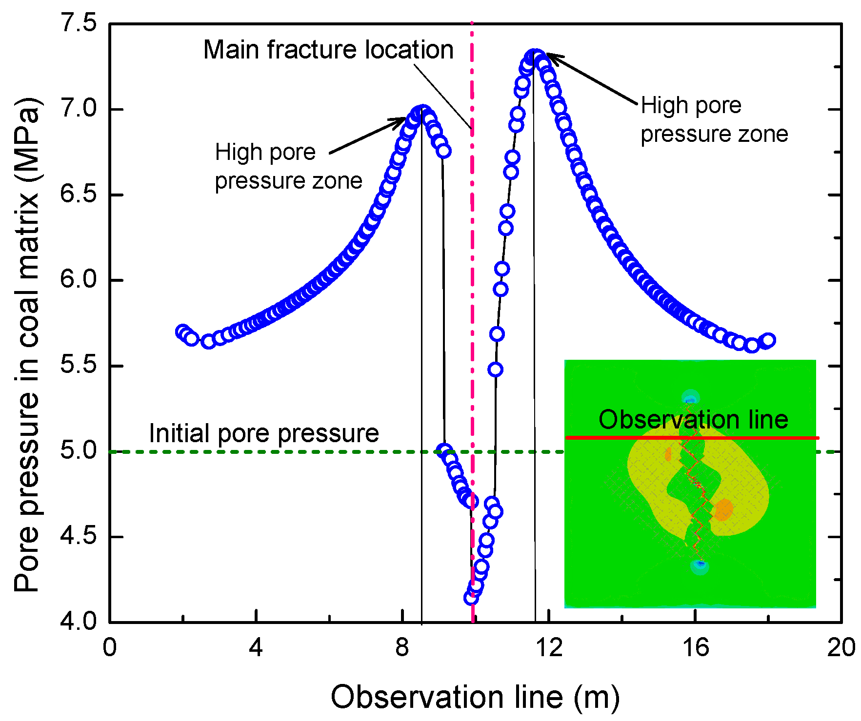
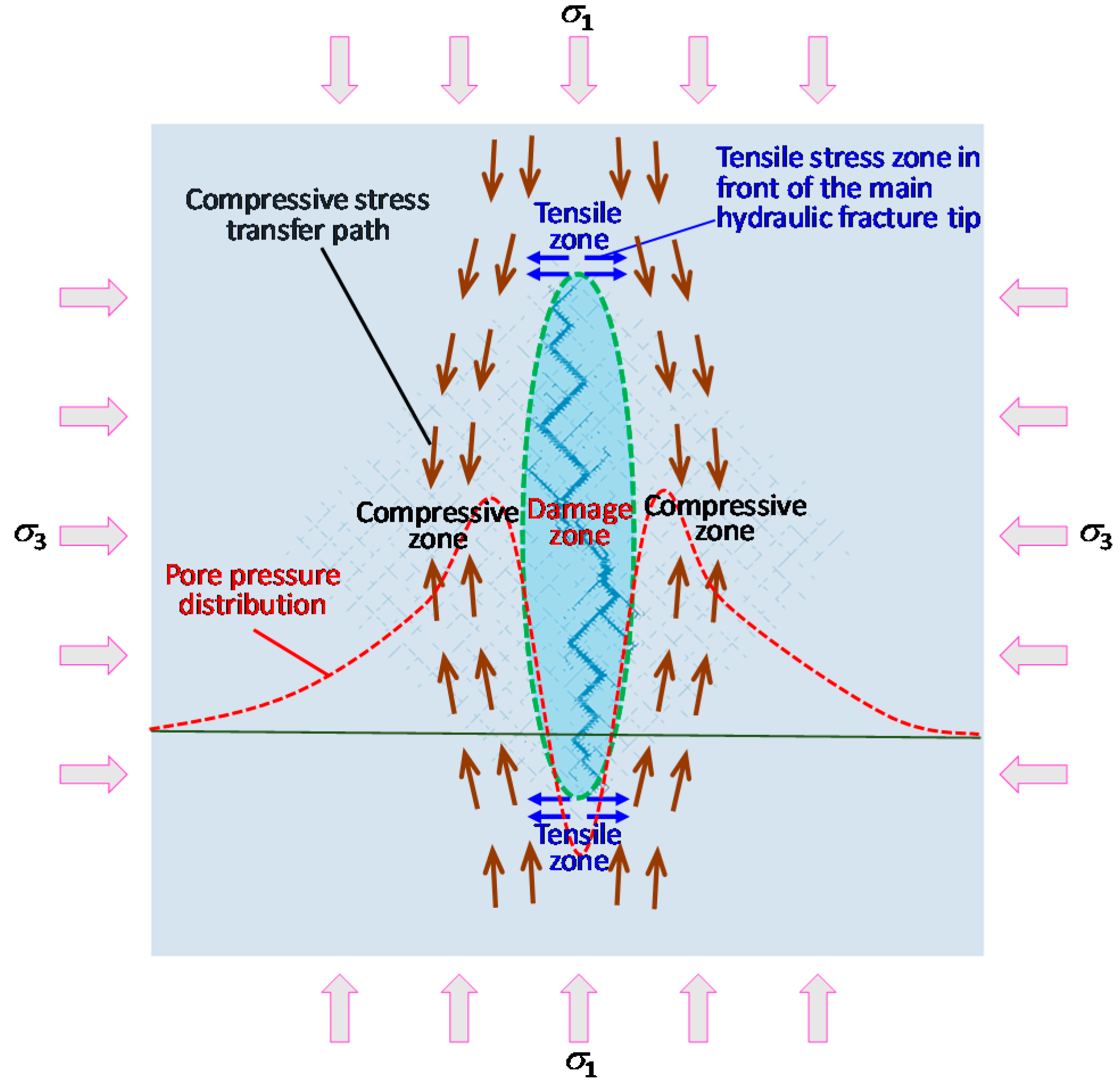
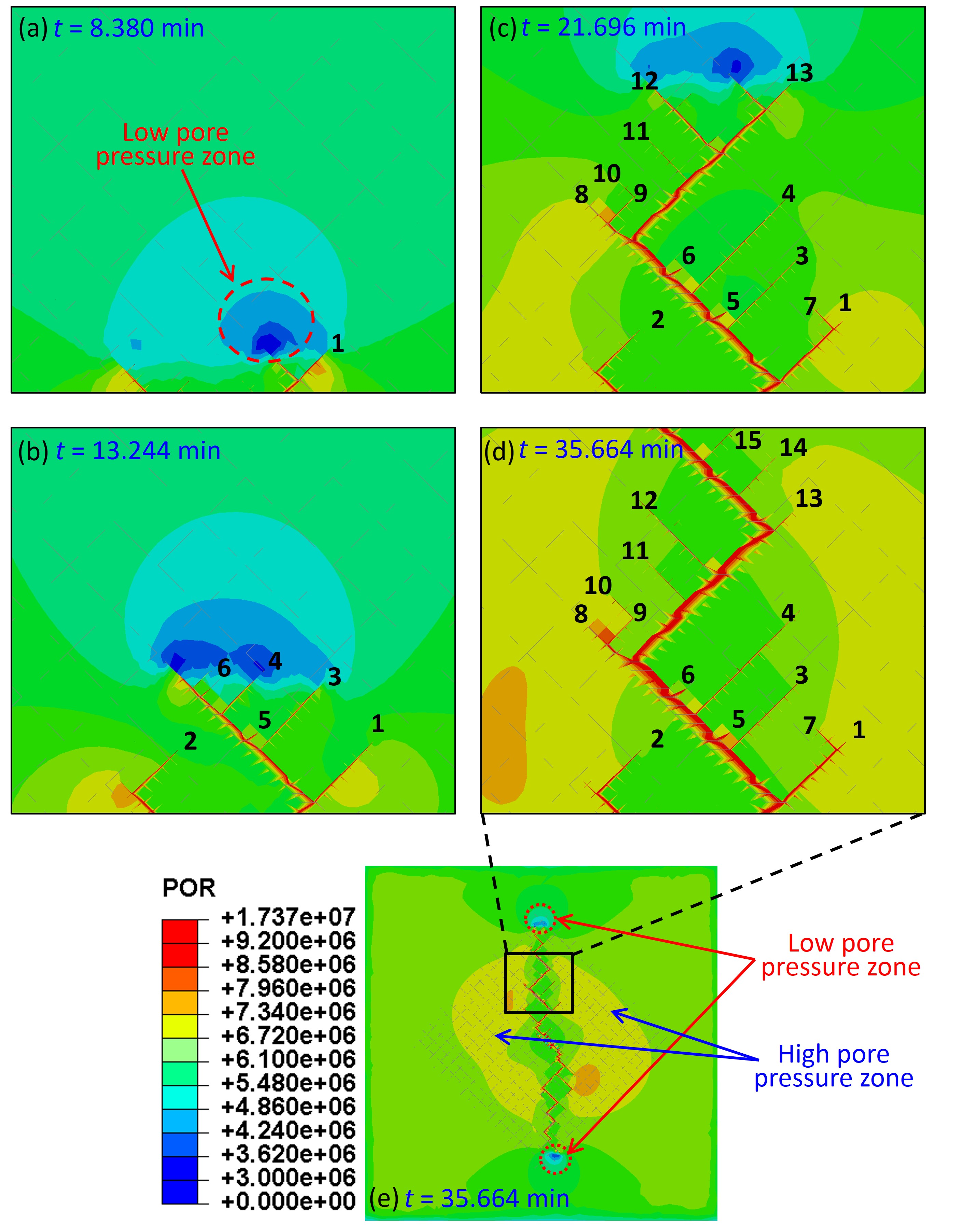
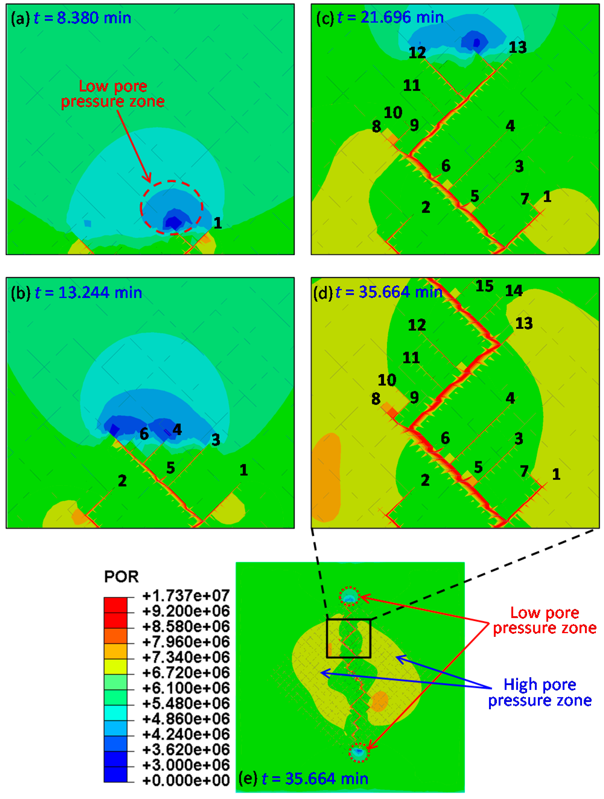
5.3. Pore Pressure Distribution Characteristics

Figure 12 also shows pore pressure distribution in the coal matrix and in hydraulic fractures. Note that there are two low pore pressure zones (the blue zones) in front of the two main fracture tips and two high pore pressure zones (the yellow zones) at both sides of the main fractures. Figure 13 shows pore pressure variation in the coal matrix on both sides of the hydraulic fractures. In Figure 13, the distance between the pore pressure peak and main fractures is approximately 1.7 m. The spindle-shaped zone, where the hydraulic fracture network is located, can be regarded as a coal damage zone that changes the transfer path of σ₁ from the far field to near field, as shown in Figure 14. The compressive stress transfer path bypasses the damage zone, resulting in a compressive stress concentration on both sides of the damage zone, which increases pore pressure. In front of the main hydraulic fractures, the coal matrix is subjected to tensile stress by hydraulic fracturing, therefore its volume tends to expand, lowering the pore pressure.

5.4. Injection Fluid Pressure

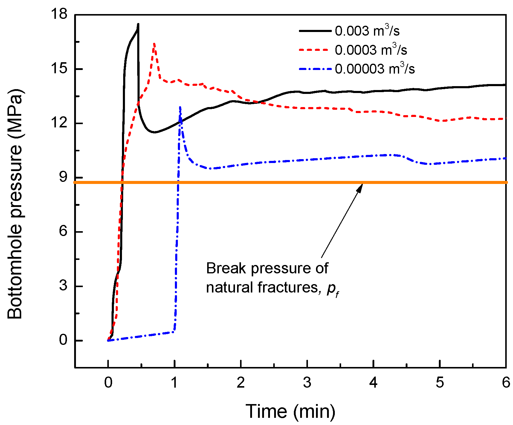
5.4.1. Effect of the Injection Rate on Bottomhole Pressure

Due to the large scale of the model (400 m²), it is difficult to consider the injection borehole profile, which is usually less than 0.04 m² in the field; thus an injection node was used instead. The bottomhole pressure variation during hydraulic fracturing was captured by the injection node. Figure 15 illustrates the bottomhole pressure variations at different injection rates under the stress condition of ${\sigma }_1$ = 17.5 MPa and ${\sigma }_3$ = 10 MPa. According to Figure 15, within the first two minutes of hydraulic fracturing, the bottomhole pressure increased rapidly due to the injection fluid impact effect, and then decreased rapidly due to hydraulic fracture initiation. The peak pressure is called the break-down pressure. After three minutes, the bottomhole pressure stabilized. The stable bottomhole pressure and the break-down pressure increased as the injection rate increased, indicating that hydraulic fracture propagation is a dynamic process. Under high injection rates, the fracture volume rate increase is slower than the injection liquid volume rate increase. This explains why the bottomhole pressure increased as the injection rate increased.

5.4.2. Break Pressure of the Discontinuous Natural Fracture

As shown in Figure 16, when the hydraulic fracture propagates along discontinuous natural fractures, the break pressure of the fracture initiation $p_f$ should overcome the sum of the normal compressive stress on discontinuous natural fractures $p_n$ and tensile strength $T_f$. That is:

$$p_f=p_n+T_f$$

(26)

Based on the stress balance principle, $p_n$ can be calculated as:

$$p_n=\frac{{\overline{\sigma }}_1+{\overline{\sigma }}_3}{2}+\frac{{\overline{\sigma }}_1-{\overline{\sigma }}_3}{2}\cos 2\theta$$

(27)

where θ is the angle between the normal direction of discontinuous natural fractures and the ${\sigma }_1$ direction. ${\overline{\sigma }}_1$ and ${\overline{\sigma }}_3$ are the effective stresses corresponding to ${\sigma }_1$ and ${\sigma }_3$, respectively. The effective stresses can be calculated using Equation (1).

By substituting Equation (27) into Equation (26), $p_f$ can be calculated as:

$$p_f=\frac{{\overline{\sigma }}_1+{\overline{\sigma }}_3}{2}+\frac{{\overline{\sigma }}_1-{\overline{\sigma }}_3}{2}\cos 2\theta +T_f$$

(28)

Equation (28) clearly states that the break pressure, $p_f$, depends on the ground stress conditions, tensile strength and direction of discontinuous natural fractures.

When ${\overline{\sigma }}_1$ = 10 MPa, ${\overline{\sigma }}_3$ = 17.5 MPa, $u_w$ (pore pressure) = 5 MPa, and θ = 45°, $p_f$ was approximately 8.755 MPa for the natural fractures, and 9.52 MPa for other parts of the discontinuous natural fractures that have the same tensile strength as the coal matrix. Compared to the ground stress, the coal seam tensile strength was very low. According to Equation (28), in deep coal seams, ${\sigma }_1$ and ${\sigma }_3$ are much greater than $T_f$, so the break pressure of discontinuous natural fractures is mainly determined by the ground stress conditions and the direction of the discontinuous natural fractures.

Hard and tight rock layers, such as geothermal energy reservoirs, have an intact rock tensile strength significantly higher than that of the joints, so hydraulic fractures tend to propagate along natural fractures. When the fracturing liquid is full of natural fractures, the fracture shear strength is drastically reduced and eventually fails. This is why the PSS model is widely used in EGS to predict fracture propagation, but is not suitable for the prediction of hydraulic fractures in deep coal seams.

Note that the above analytical process is based on the assumption of static fracturing, which is different from true dynamic fracturing. Comparing the above analytical results with the numerical simulation results in Figure 15, it can be seen that the simulated bottomhole pressure was higher than the static analytical break pressure result.

6. Conclusions

In this study, an innovative finite element meshing scheme using cohesive elements (including global cohesive element embedding and global pore pressure node sharing techniques) was used to model hydraulic fracturing. Fracture propagation and interaction with discontinuous natural fracture networks in coal seams were simulated using the cohesive element method. The hydraulic fracture network characteristics under different stress conditions, the growth process of secondary hydraulic fractures, the pore pressure distribution in coal seams, and the variation of fracturing liquid pressure were investigated in detail. The numerical simulation results show that the improved cohesive element method in this study is capable of modeling hydraulic fracturing in naturally fractured formations.

In coal seams, hydraulic fracturing generally creates a complex hydraulic fracture network that is composed of a main fracture trunk and many secondary fracture branches. The morphology of the fracture network is determined by the geo-stress field and the discontinuous natural fracture network. Under high stress difference conditions, the hydraulic fracture network is spindle-shaped, and shows a multi-level branch structure. The higher the geo-stress difference, the narrower the width of the spindle-shaped hydraulic fracture network.

The ratio of secondary fracture total length to main fracture total length was 2.11~3.62, indicating that the secondary fractures are an important part of the hydraulic fracture network. The geo-stress difference had no significant effect on the ratio of secondary fracture length to main fracture length.

The stable bottomhole pressure and the break-down pressure increased with the injection rate, indicating that fracture propagation is a dynamic process in coal seams. In deep coal seams, the break pressure of discontinuous natural fractures mainly depends on the in-situ stress field and the direction of natural fractures. The mechanism of hydraulic fracture propagation in deep coal seams is significantly different from that in hard and tight rock layers. The PSS model, which is more frequently used in EGS to predict hydraulic fracture propagation, is not suitable for deep coal seams.

References

1. Moore, T.A. Coalbed methane: A review. Int. J. Coal Geol. 2012, 101, 36–81. [Google Scholar] [CrossRef]
2. White, C.M.; Smith, D.H.; Jones, K.L.; Goodman, A.L.; Jikich, S.A.; LaCount, R.B.; DuBose, S.B.; Ozdemir, E.; Morsi, B.I.; Schroeder, K.T. Sequestration of carbon dioxide in coal with enhanced coalbed methane recovery a review. Energy Fuels 2005, 19, 659–724. [Google Scholar] [CrossRef]
3. Cai, Y.D.; Liu, D.M.; Pan, Z.J.; Yao, Y.B.; Li, J.Q.; Qiu, Y.K. Pore structure and its impact on ch4 adsorption capacity and flow capability of bituminous and subbituminous coals from northeast china. Fuel 2013, 103, 258–268. [Google Scholar] [CrossRef]
4. Cheng, W.M.; Liu, Z.; Yang, H.; Wang, W.Y. Non-linear seepage characteristics and influential factors of water injection in gassy seams. Exp. Therm. Fluid Sci. 2018, 91, 41–53. [Google Scholar] [CrossRef]
5. Zou, Q.L.; Lin, B.Q.; Liu, T.; Zhou, Y.; Zhang, Z.; Yan, F.Z. Variation of methane adsorption property of coal after the treatment of hydraulic slotting and methane pre-drainage: A case study. J. Nat. Gas Sci. Eng. 2014, 20, 396–406. [Google Scholar] [CrossRef]
6. Cheng, W.M.; Hu, X.M.; Xie, J.; Zhao, Y.Y. An intelligent gel designed to control the spontaneous combustion of coal: Fire prevention and extinguishing properties. Fuel 2017, 210, 826–835. [Google Scholar] [CrossRef]
7. Zhou, G.; Fan, T.; Ma, Y.L. Preparation and chemical characterization of an environmentally-friendly coal dust cementing agent. J. Chem. Technol. Biotechnol. 2017, 92, 2699–2708. [Google Scholar] [CrossRef]
8. Ni, G.H.; Cheng, W.M.; Lin, B.Q.; Zhai, C. Experimental study on removing water blocking effect (wbe) from two aspects of the pore negative pressure and surfactants. J. Nat. Gas Sci. Eng. 2016, 31, 596–602. [Google Scholar] [CrossRef]
9. Wright, C.A.; Tanigawa, J.J.; Mei, S.; Li, Z. Enhanced hydraulic fracture technology for a coal seam reservoir in Central China. In Proceedings of the International Meeting on Petroleum Engineering, Beijing, China, 14–17 November 1995; Society of Petroleum Engineers: Beijing, China, 1995. [Google Scholar] [CrossRef]
10. Adachi, A.; Siebrits, E.; Peirce, A.; Desroches, J. Computer simulation of hydraulic fractures. Int. J. Rock Mech. Min. Sci. 2007, 44, 739–757. [Google Scholar] [CrossRef]
11. Yuan, Z.G.; Wang, H.T.; Liu, N.P.; Liu, J.C. Simulation study of characteristics of hydraulic fracturing propagation of low permeability coal seam. Disaster Adv. 2012, 5, 717–720. [Google Scholar]
12. Hou, B.; Chen, M.; Wang, Z.; Yuan, J.B.; Liu, M. Hydraulic fracture initiation theory for a horizontal well in a coal seam. Pet. Sci. 2013, 10, 219–225. [Google Scholar] [CrossRef]
13. Li, D.Q.; Zhang, S.; Zhang, S.A. Experimental and numerical simulation study on fracturing through interlayer to coal seam. J. Nat. Gas Sci. Eng. 2014, 21, 386–396. [Google Scholar] [CrossRef]
14. Eshiet, K.I.I.; Sheng, Y. Carbon dioxide injection and associated hydraulic fracturing of reservoir formations. Environ. Earth Sci. 2014, 72, 1011–1024. [Google Scholar] [CrossRef]
15. Bredehoeft, J.; Wolff, R.; Keys, W.; Shuter, E. Hydraulic fracturing to determine the regional in situ stress field, piceance basin, colorado. Geol. Soc. Am. Bull. 1976, 87, 250–258. [Google Scholar] [CrossRef]
16. Abou-Sayed, A.; Brechtel, C.; Clifton, R. In situ stress determination by hydrofracturing: A fracture mechanics approach. J. Geophys. Res. Solid Earth 1978, 83, 2851–2862. [Google Scholar] [CrossRef]
17. Tenma, N.; Yamaguchi, T.; Zyvoloski, G. The hijiori hot dry rock test site, japan evaluation and optimization of heat extraction from a two-layered reservoir. Geothermics 2008, 37, 19–52. [Google Scholar] [CrossRef]
18. Parker, R. The rosemanowes hdr project 1983–1991. Geothermics 1999, 28, 603–615. [Google Scholar] [CrossRef]
19. Jeffrey, R.; Zhang, X.; Settari, A.; Mills, K.; Detournay, E. Hydraulic fracturing to induce caving: Fracture model development and comparison to field data. In DC Rocks 2001, The 38th US Symposium on Rock Mechanics (USRMS); American Rock Mechanics Association: Alexandria, VA, USA, 2001. [Google Scholar]
20. Van As, A.; Jeffrey, R.G. Hydraulic fracturing as a cave inducement technique at northparkes mines. In Proceedings of the Massmin 2000, Brisbane, Austrilia, 29 October–2 November 2000; Australasian Institute of Mining and Metallurgy: Parkville Victoria, Australia, 2000; Volume 2000, pp. 165–172. [Google Scholar]
21. Sun, R.J. Theoretical size of hydraulically induced horizontal fractures and corresponding surface uplift in an idealized medium. J. Geophys. Res. 1969, 74, 5995–6011. [Google Scholar] [CrossRef]
22. Harper, J.A. The marcellus shale: An old “new” gas reservoir in Pennsylvania. Pa. Geol. 2008, 38, 2–13. [Google Scholar]
23. Gandossi, L. An overview of hydraulic fracturing and other formation stimulation technologies for shale gas production. Eur. Comm. Jt. Res. Cent. Tech. Rep. 2013, 26347, 4–29. [Google Scholar]
24. Montgomery, C.T.; Smith, M.B. Hydraulic fracturing: History of an enduring technology. J. Petrol. Technol. 2015, 62, 26–40. [Google Scholar] [CrossRef]
25. McDaniel, B.W. Hydraulic fracturing techniques used for stimulation of coalbed methane wells. In Proceedings of the SPE Eastern Regional Meeting, Columbus, OH, USA, 31 October–2 November 1990; Society of Petroleum Engineers: Columbus, OH, USA, 1990. [Google Scholar] [CrossRef]
26. Sampath, K.H.S.M.; Perera, M.S.A.; Ranjith, P.G.; Matthai, S.K.; Rathnaweera, T.; Zhang, G.; Tao, X. Ch4-CO2 gas exchange and supercritical CO2 based hydraulic fracturing as cbm production-accelerating techniques: A review. J. CO2 Util. 2017, 22, 212–230. [Google Scholar] [CrossRef]
27. Ting, F.T.C. Origin and spacing of cleats in coal beds. J. Press. Vessel Technol. 1977, 99, 624–626. [Google Scholar] [CrossRef]
28. Su, X.B.; Feng, Y.L.; Chen, J.F.; Pan, J.N. The characteristics and origins of cleat in coal from western north china. Int. J. Coal Geol. 2001, 47, 51–62. [Google Scholar] [CrossRef]
29. Busse, J.; de Dreuzy, J.R.; Torres, S.G.; Bringemeier, D.; Scheuermann, A. Image processing based characterisation of coal cleat networks. Int. J. Coal Geol. 2017, 169, 1–21. [Google Scholar] [CrossRef] [Green Version]
30. Golab, A.; Ward, C.R.; Permana, A.; Lennox, P.; Botha, P. High-resolution three-dimensional imaging of coal using microfocus X-ray computed tomography, with special reference to modes of mineral occurrence. Int. J. Coal Geol. 2013, 113, 97–108. [Google Scholar] [CrossRef]
31. Rodrigues, C.F.; Laiginhas, C.; Fernandes, M.; de Sousa, M.J.L.; Dinis, M.A.P. The coal cleat system: A new approach to its study. J. Rock Mech. Geotech. Eng. 2014, 6, 208–218. [Google Scholar] [CrossRef]
32. Blanton, T.L. An experimental study of interaction between hydraulically induced and pre-existing fractures. In Proceedings of the SPE Unconventional Gas Recovery Symposium, Pittsburgh, PA, USA, 16–18 May 1982; Society of Petroleum Engineers: Pittsburgh, PA, USA, 1982. [Google Scholar] [CrossRef]
33. Dahi Taleghani, A.; Gonzalez-Chavez, M.; Yu, H.; Asala, H. Numerical simulation of hydraulic fracture propagation in naturally fractured formations using the cohesive zone model. J. Petrol. Sci. Eng. 2018, 165, 42–57. [Google Scholar] [CrossRef]
34. Yoon, J.S.; Zang, A.; Stephansson, O.; Hofmann, H.; Zimmermann, G. Discrete element modelling of hydraulic fracture propagation and dynamic interaction with natural fractures in hard rock. Procedia Eng. 2017, 191, 1023–1031. [Google Scholar] [CrossRef]
35. Damjanac, B.; Gil, I.; Pierce, M.; Sanchez, M.; Van As, A.; McLennan, J. A new approach to hydraulic fracturing modeling in naturally fractured reservoirs. In Proceedings of the 44th U.S. Rock Mechanics Symposium and 5th U.S.-Canada Rock Mechanics Symposium, Salt Lake City, UT, USA, 27–30 June 2010; American Rock Mechanics Association: Salt Lake City, UT, USA, 2010. [Google Scholar]
36. Wang, T.; Hu, W.R.; Elsworth, D.; Zhou, W.; Zhou, W.B.; Zhao, X.Y.; Zhao, L.Z. The effect of natural fractures on hydraulic fracturing propagation in coal seams. J. Petrol. Sci. Eng. 2017, 150, 180–190. [Google Scholar] [CrossRef]
37. Deng, J.Q.; Yang, Q.; Liu, Y.R.; Liu, Y.; Zhang, G.X. 3d finite element modeling of directional hydraulic fracturing based on deformation reinforcement theory. Comput. Geotech. 2018, 94, 118–133. [Google Scholar] [CrossRef]
38. Xu, L.L.; Cui, J.B.; Huang, S.P.; Tang, J.D.; Cai, L.; Yu, P. Analysis and application of fracture propagated model by hydraulic fracturing in coal-bed methane reservoir. J. China Coal Soc. 2014, 39, 2068–2074. [Google Scholar] [CrossRef]
39. Zhou, J.; Chen, M.; Jin, Y.; Zhang, G.Q. Analysis of fracture propagation behavior and fracture geometry using a tri-axial fracturing system in naturally fractured reservoirs. Int. J. Rock Mech. Min. Sci. 2008, 45, 1143–1152. [Google Scholar] [CrossRef]
40. Shilova, T.; Patutin, A.; Rybalkin, L.; Serdyukov, S.; Hutornoy, V. Development of the impermeable membranes using directional hydraulic fracturing. Procedia Eng. 2017, 191, 520–524. [Google Scholar] [CrossRef]
41. He, Q.; Suorineni, F.T.; Ma, T.; Oh, J. Effect of discontinuity stress shadows on hydraulic fracture re-orientation. Int. J. Rock Mech. Min. Sci. 2017, 91, 179–194. [Google Scholar] [CrossRef]
42. Liu, K.; Gao, D.L.; Wang, Y.B.; Yang, Y.C. Effect of local loads on shale gas well integrity during hydraulic fracturing process. J. Nat. Gas Sci. Eng. 2017, 37, 291–302. [Google Scholar] [CrossRef]
43. Yao, Y.; Wang, W.H.; Keer, L.M. An energy based analytical method to predict the influence of natural fractures on hydraulic fracture propagation. Eng. Fract. Mech. 2018, 189, 232–245. [Google Scholar] [CrossRef]
44. Tan, P.; Jin, Y.; Hou, B.; Han, K.; Zhou, Y.C.; Meng, S.Z. Experimental investigation on fracture initiation and non-planar propagation of hydraulic fractures in coal seams. Pet. Explor. Dev. 2017, 44, 470–476. [Google Scholar] [CrossRef]
45. Guo, T.K.; Rui, Z.H.; Qu, Z.Q.; Qi, N. Experimental study of directional propagation of hydraulic fracture guided by multi-radial slim holes. J. Petrol. Sci. Eng. 2018, 166, 592–601. [Google Scholar] [CrossRef]
46. Haimson, B.; Fairhurst, C. Initiation and extension of hydraulic fractures in rocks. SPE J. 1967, 7, 310–318. [Google Scholar] [CrossRef]
47. Schmitt, D.; Zoback, M. Poroelastic effects in the determination of the maximum horizontal principal stress in hydraulic fracturing tests—A proposed breakdown equation employing a modified effective stress relation for tensile failure. Int. J. Rock Mech. Min. Sci. Geomech. Abstr. 1989, 26, 499–506. [Google Scholar] [CrossRef]
48. Schmitt, D.R.; Currie, C.A.; Zhang, L. Crustal stress determination from boreholes and rock cores: Fundamental principles. Tectonophysics 2012, 580, 1–26. [Google Scholar] [CrossRef]
49. Atkinson, B.K. Fracture Mechanics of Rock; Academic Press Inc.: London, UK, 1987; Volume 2, pp. 33–45. [Google Scholar]
50. McClure, M.W.; Horne, R.N. An investigation of stimulation mechanisms in enhanced geothermal systems. Int. J. Rock Mech. Min. Sci. 2014, 72, 242–260. [Google Scholar] [CrossRef]
51. Perkins, T.; Kern, L. Widths of hydraulic fractures. J. Petrol. Technol. 1961, 13, 937–949. [Google Scholar] [CrossRef]
52. Geertsma, J.; Klerk, F.D. A rapid method of predicting width and extent of hydraulically induced fractures. J. Petrol. Technol. 1969, 21, 1571–1582. [Google Scholar] [CrossRef]
53. Nordgren, R.P. Propagation of a vertical hydraulic fracture. SPE J. 1972, 12, 306–314. [Google Scholar] [CrossRef]
54. Warpinski, N.; Wolhart, S.; Wright, C. Analysis and prediction of microseismicity induced by hydraulic fracturing. In Proceedings of the SPE Annual Technical Conference and Exhibition, San Antonio, TX, USA, 5–8 October 1997; Society of Petroleum Engineers: Richardson, TX, USA, 2001. [Google Scholar] [CrossRef]
55. Palmer, I.D.; Moschovidis, Z.A.; Cameron, J.R. Modeling shear failure and stimulation of the barnett shale after hydraulic fracturing. In Proceedings of the SPE Hydraulic Fracturing Technology Conference, The Woodlands, TX, USA, 23–25 January 2018; Society of Petroleum Engineers: College Station, TX, USA, 2007. [Google Scholar] [CrossRef]
56. Rogers, S.; Elmo, D.; Dunphy, R.; Bearinger, D. Understanding hydraulic fracture geometry and interactions in the horn river basin through dfn and numerical modeling. In Proceedings of the Canadian Unconventional Resources and International Petroleum Conference, Calgary, AB, Canada, 19–21 October 2010; Society of Petroleum Engineers: Richardson, TX, USA, 2010. [Google Scholar] [CrossRef]
57. Nagel, N.B.; Gil, I.; Sanchez-Nagel, M.; Damjanac, B. Simulating hydraulic fracturing in real fractured rocks-overcjavascript: Iterm()oming the limits of pseudo3D models. In Proceedings of the SPE Hydraulic Fracturing Technology Conference, The Woodlands, TX, USA, 23–25 January 2018; Society of Petroleum Engineers: Richardson, TX, USA, 2011. [Google Scholar] [CrossRef]
58. Weng, X.; Kresse, O.; Cohen, C.E.; Wu, R.; Gu, H. Modeling of hydraulic fracture network propagation in a naturally fractured formation. In Proceedings of the SPE Hydraulic Fracturing Technology Conference, The Woodlands, TX, USA, 23–25 January 2018; Society of Petroleum Engineers: Richardson, TX, USA, 2011. [Google Scholar] [CrossRef]
59. Wu, R.; Kresse, O.; Weng, X.; Cohen, C.E.; Gu, H. Modeling of interaction of hydraulic fractures in complex fracture networks. In Proceedings of the SPE Hydraulic Fracturing Technology Conference, The Woodlands, TX, USA, 23–25 January 2018; Society of Petroleum Engineers: The Woodlands, TX, USA, 2012. [Google Scholar] [CrossRef]
60. Renshaw, C.E.; Pollard, D.D. An experimentally verified criterion for propagation across unbounded frictional interfaces in brittle, linear elastic-materials. Int. J. Rock Mech. Min. Sci. Geomech. Abstr. 1995, 32, 237–249. [Google Scholar] [CrossRef]
61. Gu, H.; Weng, X. Criterion for fractures crossing frictional interfaces at non-orthogonal angles. In Proceedings of the 44th US Rock Mechanics Symposium and 5th US-Canada Rock Mechanics Symposium, Salt Lake City, UT, USA, 27–30 June 2010; American Rock Mechanics Association: Alexandria, VA, USA, 2010. [Google Scholar]
62. Warpinski, N.; Lorenz, J.; Branagan, P.; Myal, F.; Gall, B. Examination of a cored hydraulic fracture in a deep gas well. SPE Prod. Facil. 1993, 8, 150–158. [Google Scholar] [CrossRef]
63. Mahrer, K.D. A review and perspective on far-field hydraulic fracture geometry studies. J. Petrol. Sci. Eng. 1999, 24, 13–28. [Google Scholar] [CrossRef]
64. Jeffrey, R.G.; Zhang, X.; Thiercelin, M.J. Hydraulic fracture offsetting in naturally fractures reservoirs: Quantifying a long-recognized process. In Proceedings of the SPE Hydraulic Fracturing Technology Conference, The Woodlands, TX, USA, 5–7 February 2019; Society of Petroleum Engineers: Richardson, TX, USA, 2009. [Google Scholar] [CrossRef]
65. Khristianovic, S.; Zheltov, Y. Formation of vertical fractures by means of highly viscous fluids. In Proceedings of the 4th World Petroleum Congress, Rome, Italy, 6–15 June 1955; Volume 2, pp. 579–586. [Google Scholar]
66. Abé, H.; Mura, T.; Keer, L.M. Growth rate of a penny-shaped crack in hydraulic fracturing of rocks. J. Geophys. Res. 1976, 81, 5335–5340. [Google Scholar] [CrossRef]
67. Settari, A.; Cleary, M.P. Three-dimensional simulation of hydraulic fracturing. J. Petrol. Technol. 1984, 36, 1177–1190. [Google Scholar] [CrossRef]
68. Zhang, X.; Detournay, E.; Jeffrey, R. Propagation of a penny-shaped hydraulic fracture parallel to the free-surface of an elastic half-space. Int. J. Fract. 2002, 115, 125–158. [Google Scholar] [CrossRef]
69. Zhang, X.; Jeffrey, R.G. The role of friction and secondary flaws on deflection and re-initiation of hydraulic fractures at orthogonal pre-existing fractures. Geophys. J. Int. 2006, 166, 1454–1465. [Google Scholar] [CrossRef] [Green Version]
70. Lecampion, B.; Detournay, E. An implicit algorithm for the propagation of a hydraulic fracture with a fluid lag. Comput. Methods Appl. Mech. Eng. 2007, 196, 4863–4880. [Google Scholar] [CrossRef]
71. Dean, R.H.; Schmidt, J.H. Hydraulic-fracture predictions with a fully coupled geomechanical reservoir simulator. SPE J. 2009, 14, 707–714. [Google Scholar] [CrossRef]
72. Ji, L.J.; Settari, A.; Sullivan, R.B. A novel hydraulic fracturing model fully coupled with geomechanics and reservoir simulation. SPE J. 2009, 14, 423–430. [Google Scholar] [CrossRef]
73. Zhang, Z.; Ghassemi, A. Simulation of hydraulic fracture propagation near a natural fracture using virtual multidimensional internal bonds. Int. J. Numer. Anal. Methods Geomech. 2011, 35, 480–495. [Google Scholar] [CrossRef]
74. Chen, Z.R. Finite element modelling of viscosity-dominated hydraulic fractures. J. Petrol. Sci. Eng. 2012, 88–89, 136–144. [Google Scholar] [CrossRef]
75. Wang, J.G.; Zhang, Y.; Liu, J.S.; Zhang, B.Y. Numerical simulation of geofluid focusing and penetration due to hydraulic fracture. J. Geochem. Explor. 2010, 106, 211–218. [Google Scholar] [CrossRef]
76. Yoon, J.S.; Zimmermann, G.; Zang, A. Numerical investigation on stress shadowing in fluid injection-induced fracture propagation in naturally fractured geothermal reservoirs. Rock Mech. Rock Eng. 2015, 48, 1439–1454. [Google Scholar] [CrossRef]
77. Yoon, J.S.; Zimmermann, G.; Zang, A. Discrete element modeling of cyclic rate fluid injection at multiple locations in naturally fractured reservoirs. Int. J. Rock Mech. Min. Sci. 2015, 74, 15–23. [Google Scholar] [CrossRef]
78. Yoon, J.S.; Zimmermann, G.; Zang, A.; Stephansson, O. Discrete element modeling of fluid injection–induced seismicity and activation of nearby fault. Can. Geotech. J. 2015, 52, 1457–1465. [Google Scholar] [CrossRef] [Green Version]
79. Yoon, J.S.; Zang, A.N.; Stephansson, O. Numerical investigation on optimized stimulation of intact and naturally fractured deep geothermal reservoirs using hydro-mechanical coupled discrete particles joints model. Geothermics 2014, 52, 165–184. [Google Scholar] [CrossRef] [Green Version]
80. Al-Busaidi, A.; Hazzard, J.F.; Young, R.P. Distinct element modeling of hydraulically fractured lac du bonnet granite. J. Geophys. Res. Solid Earth 2005, 110. [Google Scholar] [CrossRef]
81. Shimizu, H. Distinct Element Modeling for Fundamental Rock Fracturing and Application to Hydraulic Fracturing. Ph.D. Thesis, Kyoto University, Kyoto, Japan, 2010. [Google Scholar]
82. Wang, T.; Zhou, W.B.; Chen, J.H.; Xiao, X.; Li, Y.; Zhao, X.Y. Simulation of hydraulic fracturing using particle flow method and application in a coal mine. Int. J. Coal Geol. 2014, 121, 1–13. [Google Scholar] [CrossRef]
83. Zhao, X.Y.; Wang, T.; Elsworth, D.; He, Y.L.; Zhou, W.; Zhuang, L.; Zeng, J.; Wang, S.F. Controls of natural fractures on the texture of hydraulic fractures in rock. J. Petrol. Sci. Eng. 2018, 165, 616–626. [Google Scholar] [CrossRef]
84. Huang, B. Research on Theory and Application of Hydraulic Fracture Weakening for Coal-Rock Mass. Ph.D. Thesis, China University of Mining Technology, Xuzhou, China, 2009. [Google Scholar]
85. Zhao, H.F.; Wang, X.H.; Liu, Z.Y.; Yan, Y.J.; Yang, H.X. Investigation on the hydraulic fracture propagation of multilayers-commingled fracturing in coal measures. J. Petrol. Sci. Eng. 2018, 167, 774–784. [Google Scholar] [CrossRef]
86. Nur, A.; Byerlee, J.D. An exact effective stress law for elastic deformation of rock with fluids. J. Geophys. Res. 1971, 76, 6414–6419. [Google Scholar] [CrossRef]
87. Zhang, G.M.; Liu, H.; Zhang, J.; Wu, H.A.; Wang, X.X. Three-dimensional finite element numerical simulation of horizontal well hydraulic fracturing. Eng. Mech. 2011, 28, 101–106. [Google Scholar]
88. Zhang, G.; Liu, H.; Zhang, J.; Biao, F.; Wu, H.; Wang, X. Simulation of hydraulic fracturing of oil well based on fluid-solid coupling equation and non-linear finite element. Acta Pet. Sin. 2009, 30, 113–116. [Google Scholar]
89. Zhang, G.M.; Liu, H.; Zhang, J.; Wu, H.A.; Wang, X.X. Mathematical model and nonlinear finite element equation for reservoir fluid-solid coupling. Rock Soil Mech. 2010, 31, 1657–1662. [Google Scholar]
90. Batchelor, G.K. An Introduction to Fluid Dynamics; Cambridge University Press: Cambridge, UK, 2000. [Google Scholar] [CrossRef]
91. Shet, C.; Chandra, N. Analysis of energy balance when using cohesive zone models to simulate fracture processes. J. Eng. Mater. Technol. 2002, 124, 440–450. [Google Scholar] [CrossRef]
92. Guo, T.K.; Qu, Z.Q.; Gong, D.Q.; Lei, X.; Liu, M. Numerical simulation of directional propagation of hydraulic fracture guided by vertical multi-radial boreholes. J. Nat. Gas Sci. Eng. 2016, 35, 175–188. [Google Scholar] [CrossRef]
93. Turon, A.; Camanho, P.P.; Costa, J.; Davila, C.G. A damage model for the simulation of delamination in advanced composites under variable-mode loading. Mech. Mater. 2006, 38, 1072–1089. [Google Scholar] [CrossRef]
94. Camanho, P.P. Failure Criteria for Fibre-Reinforced Polymer Composites. 2002. Available online: https://paginas.fe.up.pt/~stpinho/teaching/feup/y0506/fcriteria.pdf (accessed on 27 June 2018).
95. Geng, Y.G.; Tang, D.Z.; Xu, H.; Tao, S.; Tang, S.L.; Ma, L.; Zhu, X.G. Experimental study on permeability stress sensitivity of reconstituted granular coal with different lithotypes. Fuel 2017, 202, 12–22. [Google Scholar] [CrossRef]
96. Liu, R.; Li, B.; Jiang, Y.; Yu, L. A numerical approach for assessing effects of shear on equivalent permeability and nonlinear flow characteristics of 2-d fracture networks. Adv. Water Resour. 2018, 111, 289–300. [Google Scholar] [CrossRef]
97. Liu, R.; Li, B.; Jiang, Y. A fractal model based on a new governing equation of fluid flow in fractures for characterizing hydraulic properties of rock fracture networks. Comput. Geotech. 2016, 75, 57–68. [Google Scholar] [CrossRef]
98. Abaqus 2017 Documentation. Available online: https://www.3ds.com/products-services/simulia/support/documentation/ (accessed on 27 June 2018).
99. Liu, X. Mechanisms and Technical Features of Hydraulic Disturbance Method for Improvement of Coal and Rock Seams Permeability. Ph.D. Thesis, Henan Polytechnic University, Jiaozuo, China, 2015. [Google Scholar]
Figure 1. The process of generating zero-thickness cohesive elements at every solid element interface. Note that a solid element and its neighboring cohesive element are connected by sharing two common nodes, and two adjacent cohesive elements connect to each other by sharing one node.
Processes 06 00113 g001
Figure 2. (a) Schematic of the CPPE and the mesh structure by embedding discrete CPPEs; (b) the mesh structure after merging the pore pressure nodes at the same coordinates and the concept of fracturing liquid flow in fractures. Note that the CPPEs are zero-thick, and the pore pressure nodes p1, p2, p3, p4 have the same coordinates P (x, y). The fracturing liquid flow has two components: the tangential flow from one cohesive element to the next cohesive element, and the normal flow from cohesive elements to solid elements.
Processes 06 00113 g002
Figure 3. The process of creating the discontinuous fracture network.
Processes 06 00113 g003
Figure 4. Schematic of fluid flow patterns, including tangential flow and normal flow.
Processes 06 00113 g004
Figure 5. Hydraulic fracture propagation driven by fracturing liquid, and the traction–separation law for cohesive elements. In the blue zone, the cohesive elements are in a complete damage state, whereas those in red zone are in an elastic state or in an incomplete damage state.
Processes 06 00113 g005
Figure 6. The relationship between traction and separation. (a) Tensile and shear components; (b) resultant traction. In (a), E n and E s are the initial tensile stiffness and shear stiffness of CPPE, Pa/m; δ n and δ s are tensile and shear separation components, respectively. (a) interprets the concept of D, and (b) illustrates the concept of loading history (path 1 or path 2).
Processes 06 00113 g006
Figure 7. The mesh model of coal seams with discontinuous natural fracture networks. (a) shows the model size and the locations of the discontinuous natural fracture network and the injection node; (b) shows the mesh density. The fracture network zone is at the center of this model, with a size of 10 m × 10 m. The two fracture sets are orthotropic with each other, and their bisector is parallel to the principle stress direction. The fracture spacing is set to 0.5 m. The fracture network zone’s mesh consists of 10,000 pore fluid/stress elements of size 0.1 m and 20,200 CPPEs. The external zone’s mesh consists of 5612 pore fluid/stress elements of size 0.1 m to 0.6 m.
Processes 06 00113 g007
Figure 8. The preprocessing and the solving procedures of the ABAQUS/Standard solver. The module ‘soils’ was used to model hydraulic fracturing. The direct backward difference operator was used to optimize the accuracy of the continuity equation.
Processes 06 00113 g008
Figure 9. The hydraulic fracture propagation process in a discontinuous natural fracture network under different stress conditions. (a) σ 1 σ 3 = 2.5 MPa; (b) σ 1 σ 3 = 5 MPa; (c) σ 1 σ 3 = 7.5 MPa; (d) σ 1 σ 3 = 10 MPa. The red lines represent the new fractures induced by hydraulic fracturing, the blue lines represent the natural fractures with hydraulic liquid flowing, and the purple lines represent the discontinuous natural fracture network.
Processes 06 00113 g009
Figure 10. The propagation process of the main hydraulic fractures under different stress conditions. (a) σ 1 σ 3 = 2.5 MPa; (b) σ 1 σ 3 = 5 MPa; (c) σ 1 σ 3 = 7.5 MPa; (d) σ 1 σ 3 = 10 MPa.
Processes 06 00113 g010
Figure 11. The hydraulic fracture lengths under different stress conditions.
Processes 06 00113 g011
Figure 12. The numerical simulation results for the secondary hydraulic fracture growth process and pore pressure distribution. The serial numbers represent the order of secondary fracture initiation.
Processes 06 00113 g012
Figure 13. The pore pressure distribution along the observation line.
Processes 06 00113 g013
Figure 14. The schematic of pore pressure distribution around the hydraulic fractures.
Processes 06 00113 g014
Figure 15. The bottomhole pressure variations at different injection rates. The figure shows that the stable bottomhole pressure and the break-down pressure increased as the injection rate increased.
Processes 06 00113 g015
Figure 16. Schematic of the analytical model for calculating the break pressure of discontinuous natural fractures. p f is the break pressure; p n and p s are the normal compressive stress and the tangential shear stress of discontinuous natural fractures.
Processes 06 00113 g016