Membrane-Based Processes: Optimization of Hydrogen Separation by Minimization of Power, Membrane Area, and Cost

Abstract

This work deals with the optimization of two-stage membrane systems for H₂ separation from off-gases in hydrocarbons processing plants to simultaneously attain high values of both H₂ recovery and H₂ product purity. First, for a given H₂ recovery level of 90%, optimizations of the total annual cost (TAC) are performed for desired H₂ product purity values ranging between 0.90 and 0.95 mole fraction. One of the results showed that the contribution of the operating expenditures is more significant than the contribution of the annualized capital expenditures (approximately 62% and 38%, respectively). In addition, it was found that the optimal trade-offs existing between process variables (such as total membrane area and total electric power) depend on the specified H₂ product purity level. Second, the minimization of the total power demand and the minimization of the total membrane area were performed for H₂ recovery of 90% and H₂ product purity of 0.90. The TAC values obtained in the first and second cases increased by 19.9% and 4.9%, respectively, with respect to that obtained by cost minimization. Finally, by analyzing and comparing the three optimal solutions, a strategy to systematically and rationally provide ‘good’ lower and upper bounds for model variables and initial guess values to solve the cost minimization problem by means of global optimization algorithms is proposed, which can be straightforward applied to other processes.

1. Introduction

Currently, the majority of hydrogen (H₂) of industrial-grade is produced purposefully. However, H₂ can also be recovered from H₂-rich off-gas streams from petrochemical facilities or refineries, which is mostly burned as a residual gas [1]. Since industry tendencies will increase the need for more profitable sources of H₂ for a variety of applications, H₂ recovery from these off-gas streams becomes an interesting alternative to make more effective use of these existing facilities concomitantly. Some hydrogen uses or applications require ultra-high purity supply (e.g., semiconductor industry) but other applications require less pure feed stocks (e.g., hydrodesulphurization and hydrocracking). The achievable H₂ purity levels depend on the used gas separation/purification technologies.

Membrane-based gas separation for H₂ separation/purification has attracted considerable attention owing to the inherent advantages over other traditional separation technologies such as pressure swing adsorption and cryogenic adsorption processes. Membrane gas separation does not require moving parts; it has small footprint and it is a compact system; it provides operating flexibility to feed fluctuations; it demands comparatively lower energy requirement leading to lower operating costs; it does not involves chemicals, make-up, and solvents; it is easy start-up and shut-down; it requires minimal maintenance and operator attention; it allows a modular design; it requires minimal utilities; and it is easy to control. Among the main drawbacks, it can be mentioned no economy of scale due to the modular design; pretreatment of streams with particulates, organic compounds, or moisture can be difficult and/or expensive; sensitivity to chemicals can be problematic in some cases; requirement of electrical power for compression (high-quality energy) [2].

For H₂ separation, recovery and/or purification, four different membrane types have been commercialized or are being considered for development and commercialization. They are polymeric membranes, porous (ceramic, carbon, metallic) membranes, dense metal membranes, and ion-conductive membranes [3]. The polymeric membranes have achieved a comparatively high degree of industrial application and commercialization [3]. Indeed, Permea (currently a division of Air Products) was the first company to successfully use membranes for gas separation at a large industrial scale, using a polysulfone hollow-fiber (HF) membrane (commercially known as Prism) for the separation of H₂ from NH₃ reactor purge gas, in 1980 [4]. Now, there are several hundred polymeric membrane systems for H₂ separation and recovery installed by Medal/Air Liquide (Paris, France, polyimide HF), Separex/UOP (Des Plaines, IL, USA, cellulose acetate, spiral wound SW), UBE Industries (Tokyo, Japan, polyimide HF), GENERON/MG (Houston, TX, USA, tetrabromopolycarbonate HF), Permea/Air Products (Allentown, PA, USA, polysulfone HF), IMS/Praxair (Danbury, CT, USA, polyimide HF), among other companies [5]. Dense metal membranes, such as palladium and palladium-based alloys, have been commercially applied to special markets since they offer inherently a very high selectivity of H₂. Currently, a lot of research and development efforts are dedicated to porous membranes, such as ceramic and carbon compositions. Among the mentioned membrane types, ion-conducting membranes are the least studied for H₂ separating, despite many fuel cells use a proton-conducting membrane as electrolyte [3].

A lot of research was devoted to enhancing gas permeability and selectivity of membrane materials [6]. However, the separation performance has not progressed very much lately [7]. This is concluded based on the slight changes in the Robeson’s upper bound relationship for gas pairs [8], what can be considered as an indication that this separation technology has matured to a large extent. Together with the development of novel membrane materials with improved separation performances, process design becomes a key issue in the economics of membrane-based separation processes [9]. In this context, the mathematical modeling and algorithmic optimization of both the membrane module and the whole membrane-based process are of main concern for improving the performance of this separation technology. Certainly, they can be easily used for testing and providing valuable information about the sizes of the process units as well as the operating conditions of the entire process flow sheet in a short time ([10,11]).

In literature, several authors have addressed the simulation or model-based optimization of membrane-based processes for gas separation in several applications, such as gas natural treatment ([7,10,12]), CO₂ capture ([6,13,14,15]), and H₂ separation ([9,16,17]). For instance, Xu et al. [17] studied the potential applications of membrane-based processes for H₂ purification and pre-combustion CO₂ capture. They investigated single-stage and two-stage configurations, and two membrane types: CO₂ selective membranes and H₂ selective membranes (HSMs). Among other results, the authors found that a minimum cost selectivity can be obtained by fixing the membrane permeability along with the H₂ product purity level. Another important result indicated that it is difficult to reach a stable operation mode of the two-stage system with HSM because it is strongly influenced by the variation of the operating conditions. The authors highlighted the need for further investigation in this matter. By using a nonlinear mathematical programming (NLP) model implemented in GAMS (General Algebraic Modeling System) software, Zarca et al. [9] evaluated a two-stage membrane process for H₂ recovery from the tail gas generated in carbon black manufacturing process, considering two types of membranes: polymeric membranes and ionic liquid-based membranes. The authors assumed that the retentate streams are at atmospheric pressure and proposed the net present value as the objective function to be minimized. Results show that ionic liquid-based membranes are promising to achieve a H₂-rich syngas stream at a minimal cost and also to mitigate CO₂ emissions.

This work focuses on the model-based optimization of membrane-based processes to separate H₂ from a CO₂/CO/H₂/N₂ gas mixture generated in hydrocarbons processing plants to attain desired H₂ product purity levels ranging between 0.90 and 0.95 mole fraction and a H₂ recovery of 90% by minimization of the total annual cost (TAC). To this end, a NLP problem is solved using the algebraic equation-oriented optimization tool GAMS, considering simultaneously all the trade-offs existing between the model variables. Compared to the study of Zarca et al. [9], the model considers the possibility of combining vacuum pumps and compressors to create the driving forces in the membrane stages, which may lead to a reduction of the required total membrane area for a given fixed electric power level, or a reduction of the demanded electric power for a fixed value of total membrane area.

From the process systems engineering perspective, this paper contributes with an optimization model that constitutes a valuable decision-support tool to design, simulate, and optimize two-stage membrane processes for H₂ separation, as well as to elucidate the exiting techno-economic trade-offs that are difficult to distinguish at first glance.

The paper is organized as follows. Section 2 describes the studied two-stage membrane process configuration for H₂ separation. Section 3 summarizes the main model assumptions and considerations and presents the mathematical model employed in this research. Section 4 states the optimization problems to be solved. Section 5 discusses the optimization results obtained by cost minimization (Section 5.1) and total power minimization and total membrane area minimization (Section 5.2). Also, in Section 5.2, a strategy to systematically and rationally provide ‘good’ lower and upper bounds for model variables and initial guess values to solve the cost minimization problem by means of global optimization algorithms is proposed. Finally, Section 6 draws the conclusions of this work.

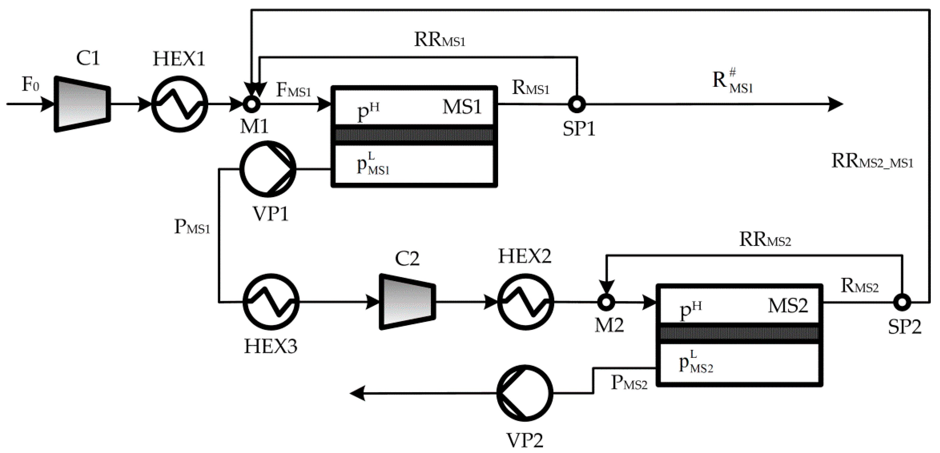
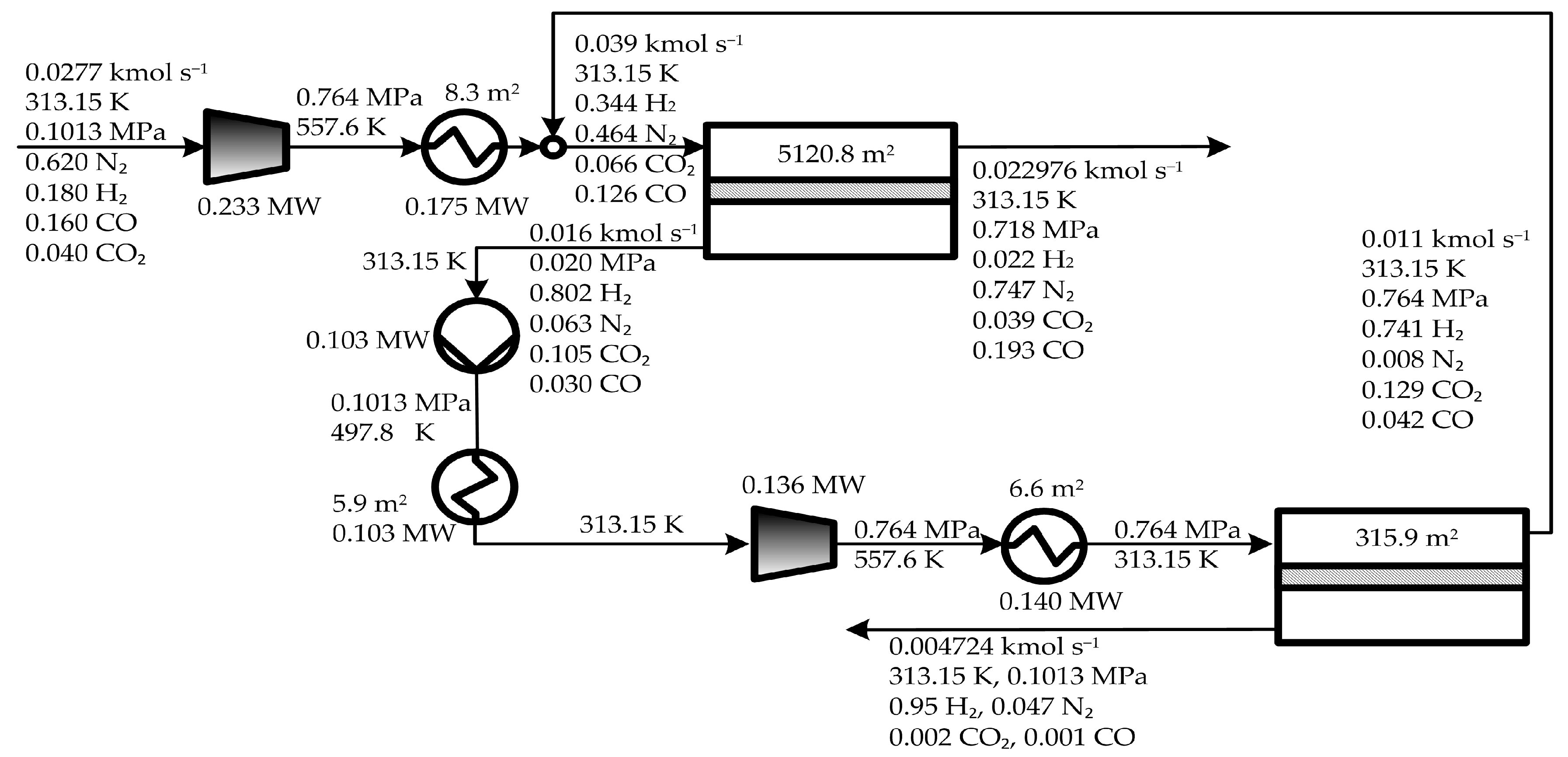
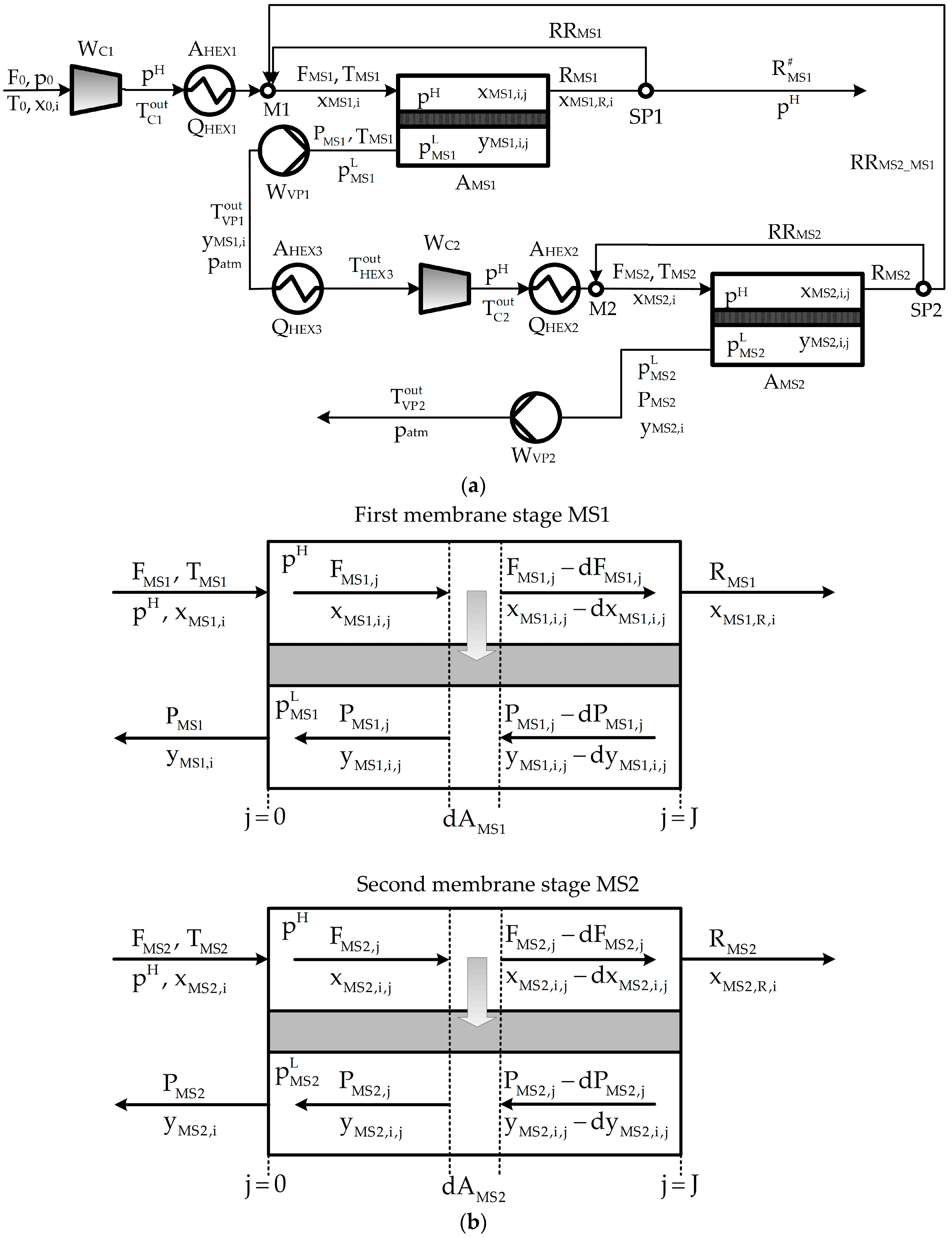
2. Process Description

As illustrated in Figure 1, the separation process proposed in this study involves two membrane units MS1 and MS2; two compressors C1 and C2; three heat exchangers HEX1, HEX2, and HEX3; and two vacuum pumps VP1 and VP2; two stream mixers M1 and M2, and two stream splitters SP1 and SP2. The incoming feed F₀ reaches the operating pressure (p^H) and temperature (T_MS) in C1 and HEX1, respectively. Then, F₀ can be optionally mixed in M1 with a fraction of the retentate obtained in MS1 (RR_MS1) and/or with a fraction of the retentate obtained in MS2 (RR_{MS2_MS1}). Afterwards, the resulting stream is fed to MS1, where it is separated into two streams: permeate stream (rich in H₂) and retentate stream. The permeate membrane side can operate under vacuum to create the driving force for component separation through the vacuum pump VP1. The permeate stream P_MS1 leaving the VP1 decreases its temperature in HEX3 and increases its pressure in C2. Afterwards, it reaches the operating temperature T_MS2 in HEX2, and it can be optionally mixed in M2 with a fraction of the retentate obtained in MS2 (RR_MS2). Finally, the resulting stream is fed to MS2, where it is separated into the corresponding retentate and permeate streams.

The best way to create the driving force for component permeation in MS i.e., the pressure difference between the retentate and permeate sides of the membrane (p^H − p^L_MS) depends on many factors such as membrane material, membrane areas, costs, and design specifications. For instance, the higher the operating pressure ratio (p^H/p^L_MS), the higher the electric power requirement but the lower the membrane area. The optimal operating pressure values p^H, p^L_MS1, and p^L_MS2 depend on the relationships between investment and operating costs not only of the compressors and vacuum pumps but also of the remaining process units. Thus, it is clear the importance of optimizing simultaneously all the techno-economic trade-offs that exist between the process variables. The proposed model includes the following three alternative ways to create the pressure difference as driving force for permeation: (i) by compressing the feed F₀ and the permeate P_MS1 by means of C1 in the first stage and C2 in the second stage (i.e., no vacuum is applied at the permeate side of the membranes); (ii) by applying vacuum at the permeate side of the membranes (i.e., no compression of the feed and permeate streams is applied); and (iii) by combining both compression and vacuum. Then, the selection i.e., presence or absence of compressors C1 and C2 and vacuum pumps VP1 and VP2 in the process configuration results from solving optimization model.

3. Process Modeling

3.1. Assumptions and Process Mathematical Model

Briefly, some main assumptions considered for modeling the membrane unit are the following: the permeability values correspond to the pure species and are not influenced by the operating pressure; steady state behavior; plug-flow pattern; constant total pressure at each membrane side. Regarding the mathematical modeling, the component mass balance in the membrane module is described by a set of algebraic equations obtained by discretization of the resulting set of ordinary differential equations employing the backward finite difference method (BFDM). The mathematical model that describes the process flow sheet illustrated in Figure 1 involves nonlinear constraints due to the presence of bilinear terms in the mass and energy balances (multiplications of concentrations and flow rates, and multiplications of enthalpies and flow rates) as well as equations to calculate costs. A complete list of the assumptions and the mathematical model used in this study to describe the membrane stages and the other process units (compressors, heat exchangers, etc.) can be found in Arias [18] and Arias et al. [15] and are also provided in Appendix A. Next, the considered cost model is presented.

3.2. Cost Model

The total annual cost (TAC, in M$ year⁻¹), capital expenditures (CAPEX, in M$), annualized capital expenditures (annCAPEX, in M$ year⁻¹), and operating expenditures (OPEX, in M$ year⁻¹) are calculated by Equations (1)–(5).

$$\mathrm{T}\mathrm{A}\mathrm{C}=\mathrm{a}\mathrm{n}\mathrm{n}\mathrm{C}\mathrm{A}\mathrm{P}\mathrm{E}\mathrm{X}+\mathrm{O}\mathrm{P}\mathrm{E}\mathrm{X}$$

(1)

$$\mathrm{a}\mathrm{n}\mathrm{n}\mathrm{C}\mathrm{A}\mathrm{P}\mathrm{E}\mathrm{X}=\mathrm{C}\mathrm{R}\mathrm{F}\cdot \mathrm{C}\mathrm{A}\mathrm{P}\mathrm{E}\mathrm{X}$$

(2)

$$\mathrm{C}\mathrm{R}\mathrm{F}=\frac{\mathrm{i}\cdot {\left(1+\mathrm{i}\right)}^{\mathrm{n}}}{{\left(1+\mathrm{i}\right)}^{\mathrm{n}}-1}$$

(3)

$$\mathrm{C}\mathrm{A}\mathrm{P}\mathrm{E}\mathrm{X}={\mathrm{f}}_1\cdot {\mathrm{C}}_{\mathrm{I}\mathrm{N}\mathrm{V}}$$

(4)

$$\mathrm{O}\mathrm{P}\mathrm{E}\mathrm{X}={\mathrm{f}}_2\cdot {\mathrm{C}}_{\mathrm{I}\mathrm{N}\mathrm{V}}+{\mathrm{f}}_3\cdot \mathrm{O}\mathrm{L}\mathrm{M}+{\mathrm{f}}_4\cdot {\mathrm{C}}_{\mathrm{R}\mathrm{M}}$$

(5)

A detailed calculation of the economic factor f₁ (4.98) in Equation (4), and f₂ (0.464), f₃ (2.45), and f₄ (1.055) in Equation (5) can be found in [15], which were estimated based on the guidelines given in [19] and [20]. In Equation (5), OPEX takes into account the manpower and maintenance costs (OLM). The total investment cost (C_INV, in M$) is calculated by Equation (6), where the investment costs of the individual process units are estimated by Equations (7)–(10):

$${\mathrm{C}}_{\mathrm{I}\mathrm{N}\mathrm{V}}={\mathrm{I}}_{\mathrm{C}1}+{\mathrm{I}}_{\mathrm{C}2}+{\mathrm{I}}_{\mathrm{V}\mathrm{P}1}+{\mathrm{I}}_{\mathrm{V}\mathrm{P}2}+{\mathrm{I}}_{\mathrm{H}\mathrm{E}\mathrm{X}1}+{\mathrm{I}}_{\mathrm{H}\mathrm{E}\mathrm{X}2}+{\mathrm{I}}_{\mathrm{H}\mathrm{E}\mathrm{X}3}+{\mathrm{I}}_{\mathrm{M}\mathrm{S}1}+{\mathrm{I}}_{\mathrm{M}\mathrm{S}2}$$

(6)

$${\mathrm{I}}_{\mathrm{H}\mathrm{E}\mathrm{X}}=0.357\cdot {\left(\frac{{\mathrm{A}}_{\mathrm{H}\mathrm{E}\mathrm{X}}}{929}\right)}^{0.6};\mathrm{HEX}:\mathrm{HEX}1,\mathrm{HEX}2,\mathrm{HEX}3$$

(7)

$${\mathrm{I}}_{\mathrm{C}}=2.788\cdot {\left(\frac{{\mathrm{W}}_{\mathrm{C}}}{2000}\right)}^{0.6};\mathrm{C}:\mathrm{C}1,\mathrm{C}2$$

(8)

$${\mathrm{I}}_{\mathrm{V}\mathrm{P}}=2.25\times 10^{-6}\cdot {\mathrm{W}}_{\mathrm{V}\mathrm{P}};\mathrm{VP}:\mathrm{VP}1,\mathrm{VP}2$$

(9)

$${\mathrm{I}}_{\mathrm{M}\mathrm{S}}=52.8\times 10^{-6}\cdot {\mathrm{A}}_{\mathrm{MS}}+0.249\cdot {\left(\frac{0.1}{55}\cdot {\mathrm{p}}^{\mathrm{H}}\right)}^{0.875}\cdot {\left(\frac{{\mathrm{A}}_{\mathrm{M}\mathrm{S}}}{2000}\right)}^{0.7};\mathrm{MS}:\mathrm{MS}1,\mathrm{MS}2$$

(10)

The raw material and utility cost (C_RM, in M$ year⁻¹) used in Equation (5) is calculated by Equation (11). It depends on the cost of electricity (C_EP), cooling water (C_CW), and membrane replacement (C_MR), which are expressed by Equations (12)–(14), respectively:

$${\mathrm{C}}_{\mathrm{R}\mathrm{M}}={\mathrm{C}}_{\mathrm{E}\mathrm{P}}+{\mathrm{C}}_{\mathrm{C}\mathrm{W}}+{\mathrm{C}}_{\mathrm{M}\mathrm{R}}$$

(11)

$${\mathrm{C}}_{\mathrm{E}\mathrm{P}}=\mathrm{c}\mathrm{r}{\mathrm{u}}_{\mathrm{E}\mathrm{P}}\cdot \mathrm{T}\mathrm{W}\cdot \mathrm{O}\mathrm{T}$$

(12)

$${\mathrm{C}}_{\mathrm{C}\mathrm{W}}=\mathrm{c}\mathrm{r}{\mathrm{u}}_{\mathrm{C}\mathrm{W}}\cdot {\mathrm{F}}_{\mathrm{C}\mathrm{W}}\cdot 1.8\times {10}^{-2}\cdot (3600\cdot \mathrm{O}\mathrm{T})$$

(13)

$${\mathrm{C}}_{\mathrm{M}\mathrm{R}}=0.2\cdot \mathrm{c}\mathrm{r}{\mathrm{u}}_{\mathrm{M}\mathrm{R}}\cdot ({\mathrm{A}}_{\mathrm{M}\mathrm{S}1}+{\mathrm{A}}_{\mathrm{M}\mathrm{S}2})$$

(14)

where the specific costs cru_EP, cru_CW, and cru_MR are, respectively, 0.072 $ kW⁻¹, 0.051 $ kg⁻¹, and 10.0 $ m⁻². An operation period (OT) of 6570 h year⁻¹ was considered.

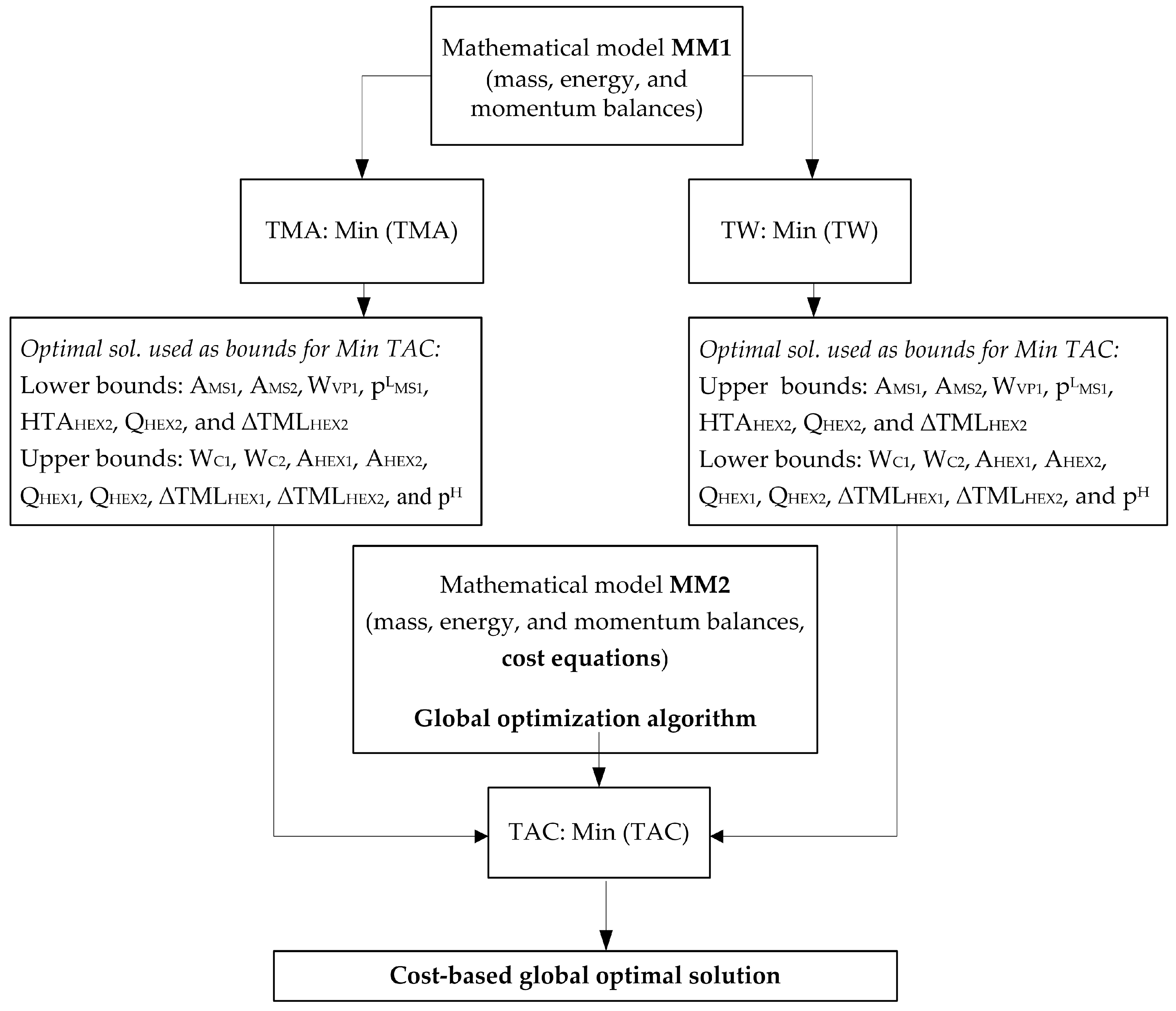
4. Problem Statement

The problem of TAC minimization considered in this work can be formally expressed as follows:

$$\begin{array}{l}\mathrm{M}\mathrm{i}\mathrm{n}\mathrm{i}\mathrm{m}\mathrm{i}\mathrm{z}\mathrm{e}\mathrm{TAC}\\ \mathrm{s}.\mathrm{t}.:\\ \{\begin{array}{l}{\mathbf{h}}_{\mathrm{s}}(\mathbf{x})=0,\forall \mathrm{s}\\ {\mathbf{g}}_{\mathrm{t}}(\mathbf{x})\le 0,\forall \mathrm{t}\\ {\mathrm{H}}_2\mathrm{recovery}=90\mathrm{\%}\\ {\mathrm{H}}_2\mathrm{purity}=\mathsf{\alpha }\\ \mathsf{\alpha }=0.90,0.91,0.92,0.93,0.94,0.95\end{array}\end{array}$$

(15)

where TAC is the objective function, x is the vector of model variables; h_s(x) refers to the mass and energy equality constraints, and correlations for physicochemical properties estimation, design specifications, and cost estimation; g_t(x) refers to inequality constraints which are employed to avoid concentration and temperature crosses in the process units. The H₂ product purity target specification is parametrically varied between 0.90 and 0.95 through the parameter α, which is a fixed value in a particular optimization run.

By solving the problem given in Equation (15), the optimization results provide:

• Minimal TAC.
• Optimal TAC distribution between the annualized capital expenditures (CAPEX) and operating expenditures (OPEX).
• Optimal sizes of the process units (membrane unit areas, heat exchanger areas, compressor and vacuum-pump power capacities).
• Optimal values of temperature, pressure, composition, and flow rate of all process streams.

The problem of minimization of the total membrane area (TMA) can be formally expressed as follows:

$$\begin{array}{l}\mathrm{M}\mathrm{i}\mathrm{n}\mathrm{i}\mathrm{m}\mathrm{i}\mathrm{z}\mathrm{e}\mathrm{TMA}\\ \mathrm{s}.\mathrm{t}.:\\ \{\begin{array}{l}{\mathbf{h}}_{\mathrm{s}}(\mathbf{x})=0,\forall \mathrm{s}\\ {\mathbf{g}}_{\mathrm{t}}(\mathbf{x})\le 0,\forall \mathrm{t}\\ {\mathrm{H}}_2\mathrm{recovery}=90\mathrm{\%}\\ {\mathrm{H}}_2\mathrm{purity}=\mathsf{\alpha }=0.90\end{array}\end{array}$$

(16)

where TMA is the objective function, which is given by Equation (A32). The model variables x and constraints h_s(x) and g_t(x) have the same meanings as in the problem given in Equation (15). In this case, the optimization problem is solved for a H₂ product purity target specification of 0.9.

Similarly, the minimization of the required total power (TW) is formulated as follows:

$$\begin{array}{l}\mathrm{M}\mathrm{i}\mathrm{n}\mathrm{i}\mathrm{m}\mathrm{i}\mathrm{z}\mathrm{e}\mathrm{TW}\\ \mathrm{s}.\mathrm{t}.:\\ \{\begin{array}{l}{\mathbf{h}}_{\mathrm{s}}(\mathbf{x})=0,\forall \mathrm{s}\\ {\mathbf{g}}_{\mathrm{t}}(\mathbf{x})\le 0,\forall \mathrm{t}\\ {\mathrm{H}}_2\mathrm{recovery}=90\mathrm{\%}\\ {\mathrm{H}}_2\mathrm{purity}=\mathsf{\alpha }=0.90\end{array}\end{array}$$

(17)

where TW is given by Equation (A34).

It can be observed that the optimization problems given in Equations (15)–(17) only differ in the objective functions to be minimized.

The complete model describing the entire process contains 3952 equations (equality and inequality constraints) and 3274 variables. It was implemented in GAMS (General Algebraic Modeling System) (release 24.2.1, GAMS Development Corporation, Fairfax, VA, USA, 2013). [21] and solved with CONOPT 3 (version 3.14W, ARKI Consulting and Development A/S, Bagsvaerd, Denmark, 2012) which is based on the generalized reduced gradient algorithm [22]. Therefore, global optimality of the discussed solutions cannot be guaranteed because of the use of a local search NLP solver. To guarantee it, a global optimization algorithm must be used instead.

5. Results and Discussion

The values of the model parameters used are taken from [9], which are listed in

Table 1. Numerical values of model parameters [9].

Parameter	Value
Feed specification
Flow rate, kmol h−1	100
Temperature, K	313.15
Pressure, kPa	101.32
Composition (mole fraction)
CO2	0.04
CO	0.16
H2	0.18
N2	0.62
Membrane material (Polymer)
Permeance (mole m−2 s−1 MPa−1)
CO2	8.444 × 10−3
CO	7.457 × 10−4
H2	2.871 × 10−2
N2	4.078 × 10−4

. In Section 5.1, optimal solutions obtained by minimizing the total annual cost for a variation range of H₂ product purity are discussed. In Section 5.2, optimal solutions obtained by minimizing the total membrane area and the electric power are presented and compared to the obtained by minimizing the total annual cost for the same design specifications.

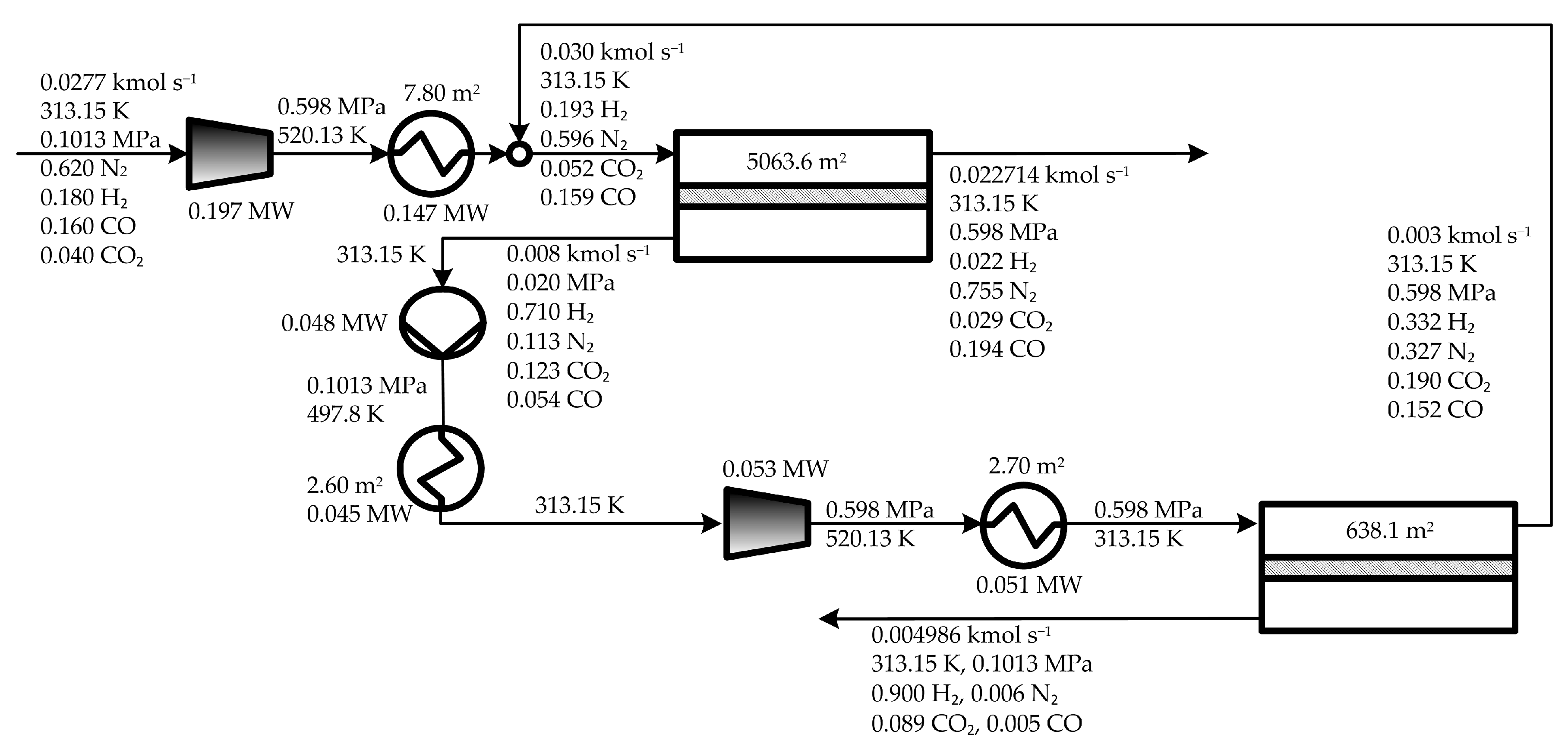
5.1. Optimal Solutions Corresponding to the Minimization of the Total Annual Cost

The main optimization results for a H₂ recovery target level of 90% and H₂ product purity target values in the range 0.90–0.95 are presented in Figure 2, Figure 3, Figure 4, Figure 5, Figure 6, Figure 7, Figure 8, Figure 9 and Figure 10.

Figure 2a shows that the total annual cost (TAC) value increases as the H₂ purity increases since the H₂ permeate flow rate in the first stage increases to satisfy the increased purity, as shown in Figure 7, Figure 8 and Figure 9 for H₂ product purity levels of 0.90, 0.91, and 0.94, respectively. For instance, compared to 0.90 H₂ product purity, the minimum TAC value obtained for 0.95 H₂ purity increases by 26.2% (from 1.764 to 2.227 M$ year⁻¹) as consequence of the increase of both the OPEX value by 25.1% (from 1.095 to 1.370 M$ year⁻¹) and the annCAPEX value by 28.1% (from 0.669 to 0.857 M$ year⁻¹). On the other hand, it can be observed in Figure 2b that the contribution ratio between OPEX and annCAPEX to the TAC remains almost constant with increasing H₂ purity values. Certainly, the contribution of OPEX to the TAC varies slightly from 62.1% to 61.6% for H₂ product purity values of 0.90 and 0.95, respectively.

Also, Figure 2a shows that an increment of H₂ product purity in 0.01 determines different percentage variations in costs depending on the purity level itself. For instance, an increment of H₂ purity from 0.90 to 0.91 implies an increase of TAC in 3.74 × 10⁻² M$ year⁻¹ (from 1.764 to 1.802 M$ year⁻¹, i.e., 2.1%) while the same increment from 0.94 to 0.95 implies an increase of TAC in 0.173 M$ year⁻¹ (from 2.054 to 2.227 M$ year⁻¹, i.e., 8.4%).

By comparing Figure 3 and Figure 4 it can be observed that an increment of H₂ purity from 0.90 to 0.94 increases the permeate flow rate (from 0.008 to 0.013 kmol s⁻¹) and H₂ concentration (from 0.710 to 0.774 mole fraction) in the first stage, but decreases the permeate flow rate in the second stage (from 4.986 × 10⁻³ to 4.774 × 10⁻³ kmol s⁻¹). It is interesting to note that, in order to reach these flow rate values and H₂ purities, the electric power requirement by compressors and vacuum pump increases in total 0.108 MW (0.026 MW, 0.049 MW, and 0.033 MW in C1, C2, and VP1, respectively) while the optimal total membrane area decreases 332.1 m² (58.0 m² and 274.1 m² in the first and second stage, respectively). Thus, the optimal cost-based trade-offs indicate that it is more beneficial to increase the total electrical power (to operate the process at higher operating pressure values p^H as shown in Figure 5) rather than to increase the total membrane area.

However, the comparison of Figure 4 and Figure 6 shows that a different trade-off is established between the required total electric power and total membrane area when the H₂ product purity is increased from 0.94 to 0.95. In this case, it is necessary to increase both the total membrane area about 67.0 m² (from 5369.7 to 5436.7 m²) and the electric power about 0.065 MW (from 0.406 to 0.471 MW) in order to satisfy a desired H₂ purity of 0.95. It is interesting to note that the increase of the total membrane area results from an increase of the area of the first stage in 115.2 m² and a decrease of the area of the second stage in 48.2 m², which is a trend opposite to the one observed when the H₂ purity increases from 0.90 to 0.94 (Figure 3 and Figure 4), where the area of MS1 and MS2 decreases and increases, respectively, with increasing purity levels. This behavior can be better understood by observing in Figure 7 the individual variation of the area of both membranes with increasing product purity levels. This figure interestingly shows that the curve of the membrane area corresponding to MS1 has a minimum value at a H₂ purity value of 0.93, and that the one corresponding to MS2 decreases practically linearly in the studied purity variation range. This is one of the reasons of why dissimilar trade-offs between the same process variables are established at different values of H₂ purity levels.

These results clearly show the advantages of having an optimization mathematical model, mainly when both high recovery and purity levels are simultaneously targeted using membranes in gas separation processes. Certainly, it allows identifying the critical trade-offs that are otherwise difficult to distinguish at first glance.

Regarding the optimal contribution of each process unit to the total investment, Figure 8a shows that the compressor C1 used for compressing the feed in the first stage is the largest contributor; its contribution increases practically linearly with increasing H₂ product purity values. It is followed by the compressor C2 used in the second stage for compressing the permeate leaving the vacuum pump VP1. In contrast to C1, the contribution of C2 increases exponentially with increasing H₂ product purity values, showing a behavior similar to the one observed for the optimal high operating pressure p^H values (Figure 5). The third contributor to the total investment is the membrane area required in the first stage A_MS1, with an investment that remains almost constant with increasing H₂ product purities. The vacuum pump VP1 is the fourth contributor, whose investment increases more importantly at high H₂ purity values. The contributions of the remaining process units are comparatively less important or practically insignificant.

Regarding the distribution of raw material and utility cost C_RM shown in Figure 8b, the cost of electricity for running the compressors and the vacuum pump is by far the major contributor, and it increases more rapidly with increasing H₂ product purity levels.

Figure 9 clearly shows that the increases in electric power required by the compressor of the second stage C2 and the vacuum pump VP1 are more significant than the increase in electric power required by compressor C1 in the first stage.

Finally, Figure 10 shows the heat transfer areas of HEX2 and HEX3 (Figure 10a) and their corresponding heat loads (Figure 10b) increase in greater proportion than those corresponding to HEX1, with increasing H₂ purity levels. The area increases in HEX1 and HEX3 are mainly due to the increase in the compression ratio of the compressors which rises their outlet temperatures, thus requiring more area for heat transfer to reach the operating temperature of the stages (313.15 K). On the other hand, the increase of the heat transfer area of HEX2 (located after the vacuum pump VP1) and its corresponding heat load is only due to the increase in the permeate flow rate since the first stage operates with a vacuum level of 0.020 MPa, what implies the same pressure ratio (5.065) and, therefore, the same output temperature (497.8 K) for all the H₂ product purity levels.

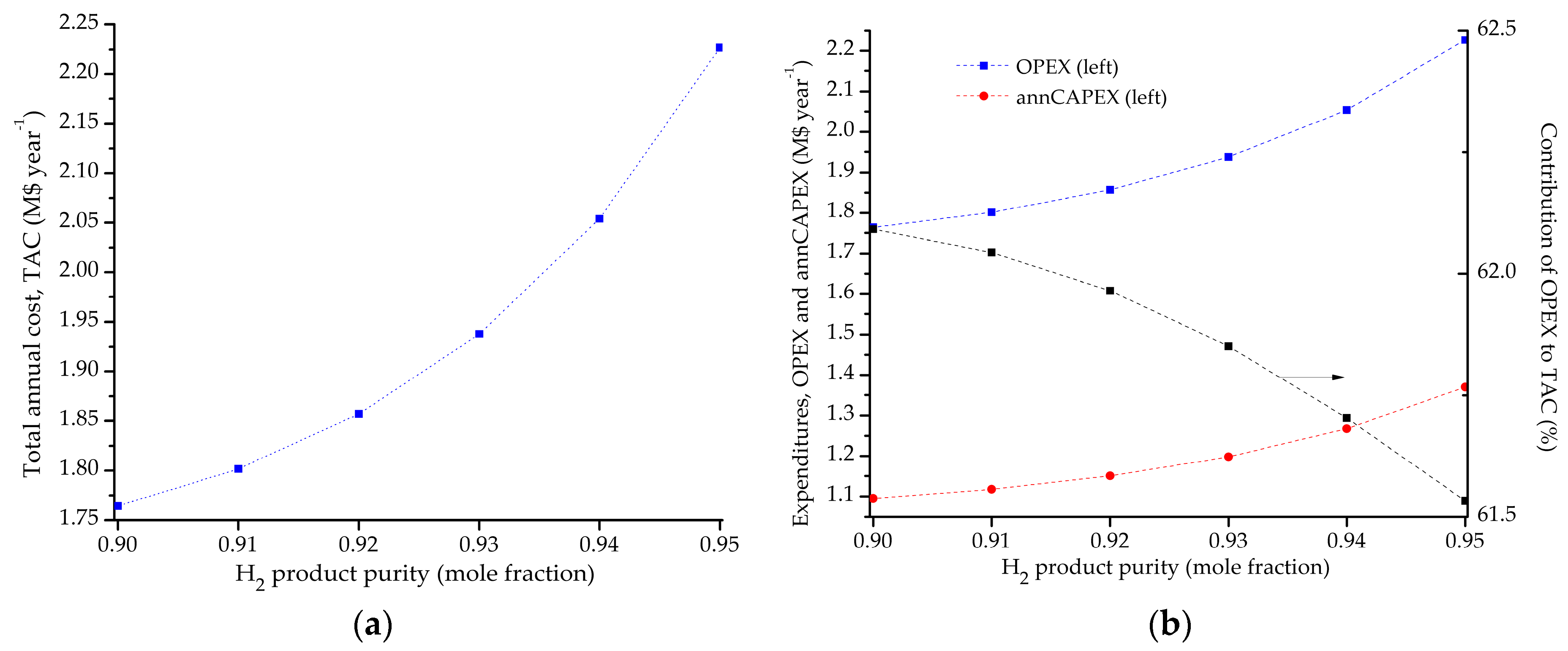
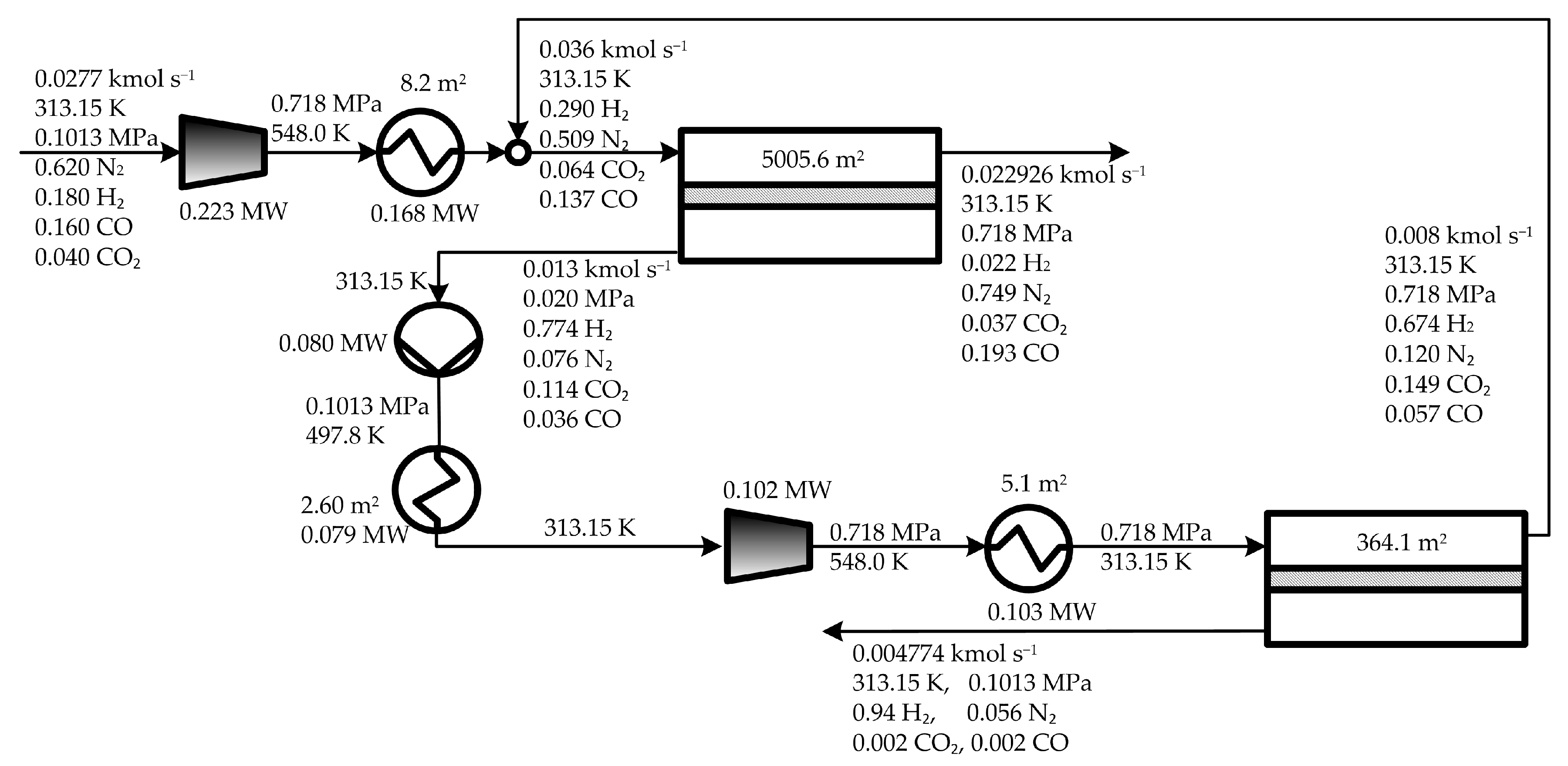
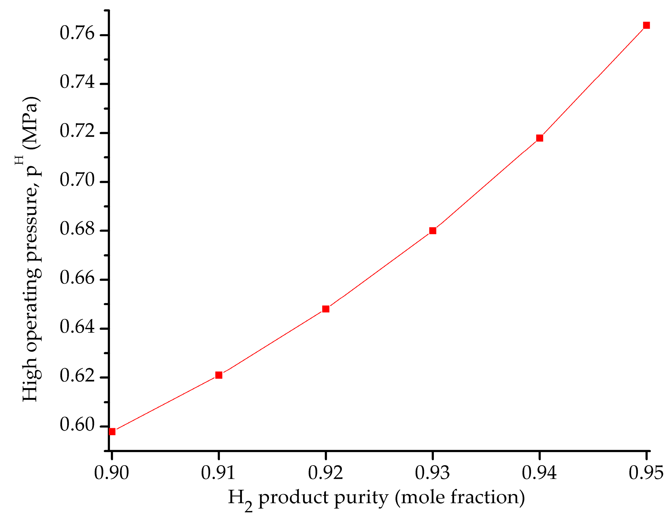
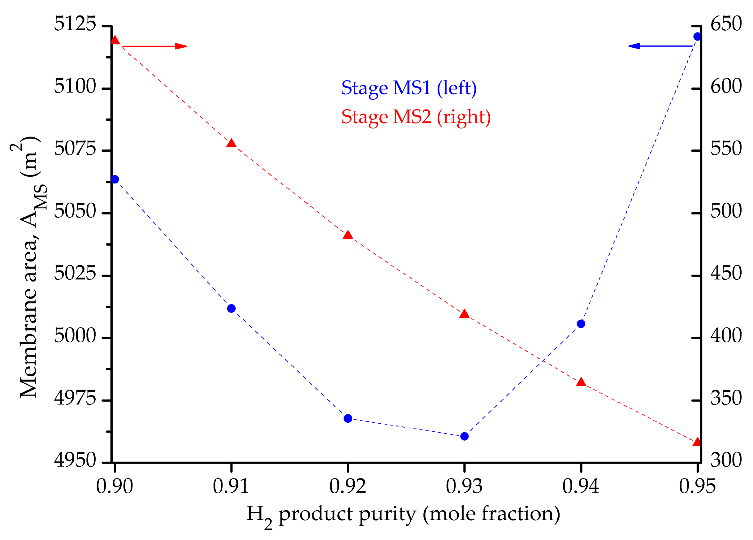
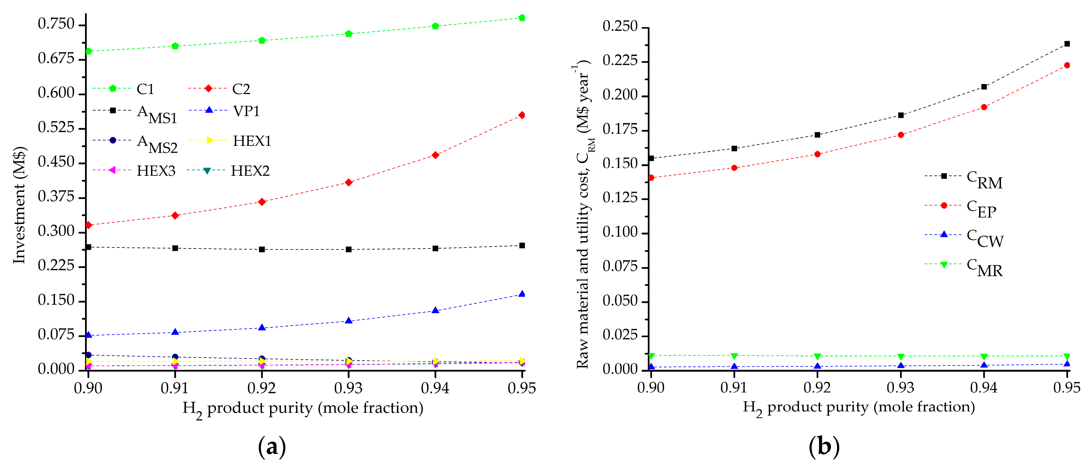
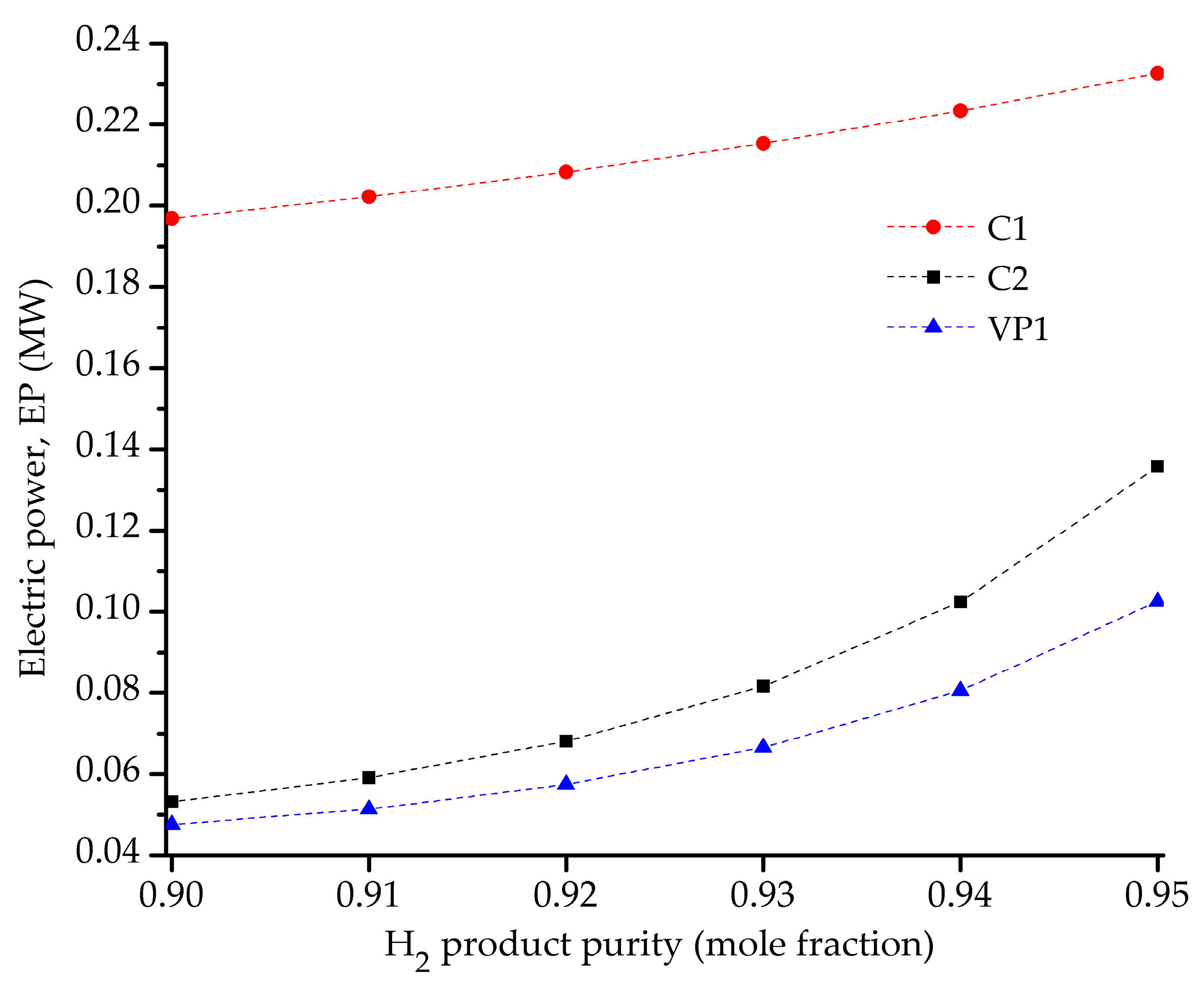
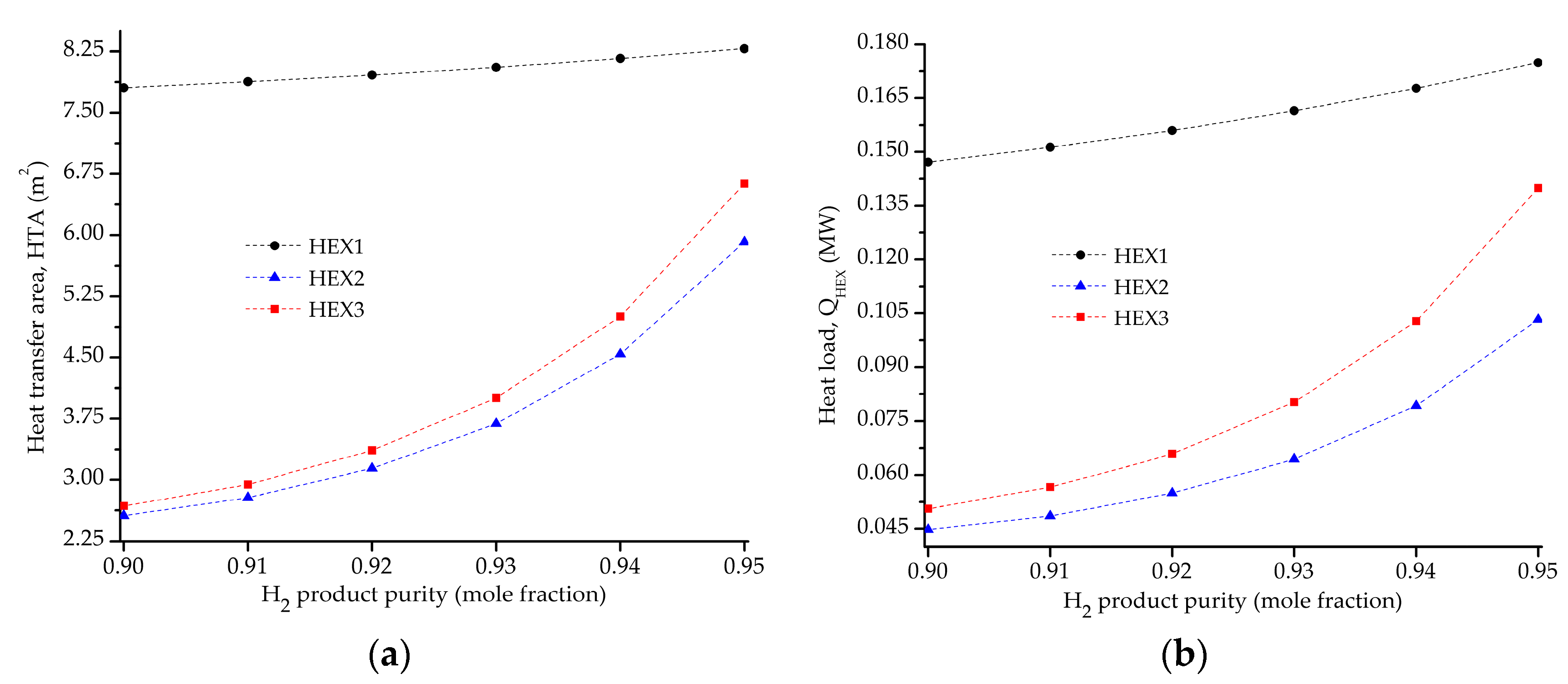
5.2. Influence of the Objective Functions on the Optimal Design and Operating Conditions

As introduced earlier, the aim of this section is to study the influence of the objective functions that are minimized on the optimal solutions and to see how these solutions can be properly used in global optimization algorithms. To this end, the same process and cost mathematical models are used to solve the optimization problems that result by considering the two remaining objective functions: minimization of the total membrane area TMA (Equation (A32)) and minimization of the total power TW (Equation (A34)).

The optimization results obtained for the three objective functions are compared in

Table 2. Minimization of TAC, TMA, and TW for 90% H₂ recovery and 0.90 H₂ product purity: Costs. (TAC: total annual cost; TMA: total membrane area; TW: total power).

Cost Item	Min TMA (osTMA)	Min. TAC (osTAC)	Min TW (osTW)
TAC (M$ year−1)	1.851	1.764	2.116
OPEX (M$ year−1)	1.158	1.095	1.262
annCAPEX (M$ year−1)	0.692	0.669	0.853
CINV (M$)	1.481	1.431	1.826
IC1	0.852	0.694	0.489
IC2	0.365	0.316	0.274
IMA_MS1	0.134	0.269	0.831
IVP1	6.93 × 10−2	7.67 × 10−2	0.1043
IHEX1	2.19 × 10−2	2.03 × 10−2	0.018
IMA_MS2	1.84 × 10−2	3.40 × 10−2	8.49 × 10−2
IHEX3	1.10 × 10−2	1.07 × 10−2	1.14 × 10−2
IHEX2	9.87 × 10−3	1.04 × 10−2	1.26 × 10−2
CRM (M$ year−1)	0.193	0.155	0.139
CE	0.183	0.141	0.102
CMR	5.71 × 10−3	1.14 × 10−2	3.46 × 10−2
CCW	3.66 × 10−3	2.79 × 10−3	2.06 × 10−3

(in terms of costs) and

Table 3. Minimization of TAC, TMA, and TW for 90% H₂ recovery and 0.90 H₂ product purity: Process-unit sizes and operating conditions.

Cost Item	Min TMA (osTMA)	Min. TAC (osTAC)	Min TW (osTW)
TMA (m2)	2854.23	5701.66	17316.96
MAMS1	2510.80	5063.60	15714.90
MAMS2	343.43	638.06	1602.06
TW (MW)	0.387	0.298	0.216
WC1	0.277	0.197	0.110
WC2	6.75 × 10−2	5.32 × 10−2	4.20 × 10−2
WVP1	4.29 × 10−2	4.75 × 10−2	6.46 × 10−2
HTAHEX1 (m2)	8.839	7.802	6.378
HTAHEX2 (m2)	2.305	2.6	3.5
HTAHEX3 (m2)	2.813	2.680	2.997
QHEX1 (MW)	0.210	0.147	8.09 × 10−2
QHEX2 (MW)	4.10 × 10−2	4.50 × 10−2	6.00 × 10−2
QHEX3 (MW)	6.68 × 10−2	5.05 × 10−2	3.80 × 10−2
∆TMLHEX1 (K)	85.533	67.908	45.676
∆TMLHEX2 (K)	62.871	62.871	61.236
∆TMLHEX3 (K)	85.533	67.908	45.676
pH (MPa)	1.01320	0.59834	0.30396
pLMS1 (MPa)	2.00 × 10−2	2.00 × 10−2	2.10 × 10−2
pLMS2 (MPa)	0.10132	0.10132	0.10132

(in terms of process-unit sizes and operating conditions). The optimal solutions resulting from the minimization of TAC, minimization of TMA, and minimization of TW are hereafter referred as ‘osTAC’, ‘osTMA’, and ‘osTW’, respectively.

Table 2 shows that the TAC value obtained in osTAC is 4.7% and 16.6% lower than those obtained in osTMA and osTW, respectively; while the OPEX value obtained in osTAC is 5.4% and 13.2% lower than the respective ones obtained in osTMA and osTW. The annCAPEX value obtained in osTAC is 3.4% and 21.6% lower than the obtained in osTMA and osTW, respectively. Table 3 shows that the minimal TMA value required by the process in solution osTMA is 2854.23 m², which is, respectively, 49.9% and 83.5% lower than the value obtained in osTAC and osTW, but the electric power required in osTMA is 30.2% and 79.1% higher than the required in osTAC and osTW, respectively. Table 3 shows that the minimization of TMA (2854.23 m²) implies the highest TW value (0.387 MW) reaching the upper bound for p^H (1.01320 MPa). Also, Table 3 shows that the minimization of TW (0.216 MW) implies the highest TMA value (17,316.96 m²).

So far, the optimal solutions obtained by minimization of three different objective functions by using a local search algorithm have been presented. Next, the features of these solutions are considered to propose a systematic strategy for providing bounds for model variables in global optimization (GO) methods. The application of GO algorithms using deterministic mathematical models allows to obtain a solution for a given global optimality tolerance. As is well known from a computational point of view, the calculation of good lower and upper bounds is crucial for the success of any GO algorithm [23]. Sherali et al. [24] proposed an improved method to develop tight linear relaxations to calculate global lower bounds for a design problem associated with the water distribution network. To this end, they exploited the characteristics (nature) of the nonlinear constraints such as monotonicity and the convex-concave functions. The proposed method allowed obtaining novel network designs as well as identifying promising search sub-regions. Ruiz and Grossmann [25] proposed an efficient procedure to find strong bounds in generalized disjunctive (GDP) problems. Based on the theory associated with disjunctive programming, they proposed several rules to generate more efficiently new relaxations to predict strong bounds for the global optimum. The proposed procedure considerably enhanced the computational cost because it leads to a significant reduction of the number of nodes to evaluate by the branch-and-bound methods. Kirst et al. [26] presented a comprehensive discussion about the difficulties to determine good bounds in branch-and-bound methods for GO of mathematical models involving non-convex constraints. Also, they proposed a consistent way to calculate bounds by perturbing infeasible points to feasible ones by iterating along Mangasarian-Fromovitz directions. The perturbations were done using optimal solutions obtained from linear optimization problems.

Taking into consideration the above comments and the characteristics of the optimal solutions reported in Table 2 and Table 3, it is interesting to investigate how the information provided by the optimal solutions corresponding to the minimization of the total membrane area (osTMA) and the total power (osTW) can be used in GO algorithms to solve the problem of minimization of the total annual cost, and therefore, to guarantee the optimality of the optimal solutions for the two-stage membrane process for H₂ separation studied in this paper (which in fact can be straightforward applied to other processes). More precisely, in order to determine tight variable bounds, the idea behind is to use the information predicted by the same model of the process but considering two different situations: membrane area minimization and power minimization, which represent two extremes that can be used efficiently to narrow the feasible region of the cost optimization problem. Unlike other works, it is here intended to establish a systematic bounding procedure using information inherent to the process obtained in a rational way instead of exploiting the nature of the associated constraints (at the beginning of the methodology) without applying any rational criterion.

By comparing numerically the results presented in Table 2 and Table 3, it can be observed that the optimal values corresponding to osTMA and osTW provide `good’ lower/upper bounds for decision variables to obtain the solution osTAC to global optimality. Thus, it is possible to propose a `pre-processing’ phase to systematically and rationally provide good lower and upper bounds to solve the cost minimization problem to global optimality. The schematic of the proposed pre-processing methodology (Figure 11) shows that two optimization problems (which only differ on the objective function) are solved by using a same mathematical model of the process without including cost constraints (model MM1). The first step is to solve the minimization of TMA; the optimal values of A_MS1, A_MS2, W_VP1, p^L_MS1, HTA_HEX2, Q_HEX2, and ∆TML_HEX2 are provided as lower bounds to solve the minimization of TAC while the optimal values of W_C1, W_C2, A_HEX1, A_HEX2, Q_HEX1, Q_HEX2, ∆TML_HEX1, ∆TML_HEX2, and p^H are provided as upper bounds. The second step consists on the minimization of TW; the optimal values of W_C1, W_C2, A_HEX1, A_HEX2, Q_HEX1, Q_HEX2, ∆TML_HEX1, ∆TML_HEX2, and p^H are now provided as lower bounds while the values of A_MS1, A_MS2, W_VP1, p^L_MS1, HTA_HEX2, Q_HEX2, and ∆TML_HEX2 as upper bounds. Thus, if the minimization of TMA provides a lower bound for a given decision variable, then the minimization of TW provides an upper bound for it, and vice versa. It is said that the pre-processing phase provides bounds in a rational way because they represent limits for the sizes of the pieces of equipment and/or process operation conditions. They can be used to identify smaller search spaces for the cost optimization problem and reduce the number of iterations, and consequently, the computing time. In addition, one of the two solutions (osTMA or osTW) can be used as an initial guess point in the global optimization algorithm because they are both feasible solutions for the cost optimization problem, thus facilitating the model convergence.

6. Conclusions

This paper presented the optimization results of a two-stage membrane system for H₂ separation by minimization of the total annual cost, the total membrane area, and the total electric power as single objective functions, employing a nonlinear mathematical model implemented in GAMS environment.

One of the cost optimization results showed that the optimal trade-off existing between the total membrane area and the total electric power depends on the H₂ product purity target levels. In fact, it was found that different trade-offs are established between the required total electric power and the total membrane area when the H₂ product purity is increased from 0.90 to 0.94 and from 0.94 to 0.95. In the former case, the total electric power increases and the total membrane area decreases with the increasing of the H₂ purity. The optimal cost-based trade-offs indicated that it is more beneficial to increase the total electric power (to operate the process at higher operating pressure values) rather than to increase the total membrane area. However, in the last case, it was observed that both the total membrane area and the total electric power increase with the increasing of the H₂ product purity.

The proposed mathematical model was solved considering the three aforementioned objective functions, and the obtained solutions were compared. It was observed that the optimal values obtained by minimizing the total membrane area and the total electric power (as single objectives) are `good’ bounds when the total annual cost is intended to be minimized to global optimality. By inspecting each one of the solutions, it was proposed a `pre-processing’ phase to systematically and rationally provide good lower and upper bounds to solve the minimization of the total annual cost to global optimality, which is important aspect in optimization.

From the process system engineering perspective, this paper contributes with an optimization model that constitutes a valuable decision-support tool for designing, simulating, and optimizing two-stage membrane processes for hydrogen separation, as well as elucidating the exiting techno-economic trade-offs that are difficult to distinguish at first glance.

In a next paper, global optimization will be addressed by using the bounding strategy here proposed. Also, the model will be further extended to incorporate the variation of the permeability of the membrane with the aging of the material.

References

1. Benson, J.; Celin, A. Recovering hydrogen—And profits—From hydrogen-rich offgas. Chem. Eng. Prog. 2018, 114, 55–59. [Google Scholar]
2. Favre, E. Polymeric Membranes for Gas Separation. In Comprehensive Membrane Science and Engineering; Drioli, E., Giorno, L., Eds.; Elsevier: Amsterdam, The Netherlands, 2010; Volume II, pp. 155–212. ISBN 978-0-444-53204-6. [Google Scholar]
3. Edlund, D. Hydrogen Membrane Technologies and Application in Fuel Processing. In Hydrogen and Syngas Production and Purification Technologies; Liu, K., Song, C., Subramani, V., Eds.; Wiley-Blackwell: Hoboken, NJ, USA, 2009; pp. 357–384. ISBN 978-0-471-71975-5. [Google Scholar]
4. Baker, R. Membrane Technology in the Chemical Industry: Future Directions. In Membrane Technology; Pereira Nunes, S., Peinemann, K.-V., Eds.; Wiley-Blackwell: Hoboken, NJ, USA, 2001; pp. 268–295. ISBN 978-3-527-60038-0. [Google Scholar]
5. Shalygin, M.G.; Abramov, S.M.; Netrusov, A.I.; Teplyakov, V.V. Membrane recovery of hydrogen from gaseous mixtures of biogenic and technogenic origin. Int. J. Hydrog. Energy 2015, 40, 3438–3451. [Google Scholar] [CrossRef]
6. Ramírez-Santos, Á.A.; Bozorg, M.; Addis, B.; Piccialli, V.; Castel, C.; Favre, E. Optimization of multistage membrane gas separation processes. Example of application to CO2 capture from blast furnace gas. J. Membr. Sci. 2018, 566, 346–366. [Google Scholar] [CrossRef]
7. Ohs, B.; Lohaus, J.; Wessling, M. Optimization of membrane based nitrogen removal from natural gas. J. Membr. Sci. 2016, 498, 291–301. [Google Scholar] [CrossRef]
8. Robeson, L.M. The upper bound revisited. J. Membr. Sci. 2008, 320, 390–400. [Google Scholar] [CrossRef]
9. Zarca, G.; Urtiaga, A.; Biegler, L.T.; Ortiz, I. An optimization model for assessment of membrane-based post-combustion gas upcycling into hydrogen or syngas. J. Membr. Sci. 2018, 563, 83–92. [Google Scholar] [CrossRef]
10. Ahmad, F.; Lau, K.K.; Shariff, A.M.; Murshid, G. Process simulation and optimal design of membrane separation system for CO2 capture from natural gas. Comput. Chem. Eng. 2012, 36, 119–128. [Google Scholar] [CrossRef]
11. Chowdhury, M.H.M.; Feng, X.; Douglas, P.; Croiset, E. A new numerical approach for a detailed multicomponent gas separation membrane model and AspenPlus simulation. Chem. Eng. Technol. 2005, 28, 773–782. [Google Scholar] [CrossRef]
12. Ghasemzadeh, K.; Jafari, M.; sari, A.; Babalou, A.A. Performance investigation of membrane process in natural gas sweetening by membrane process: modeling study. Chem. Prod. Process Model. 2016, 11, 23–27. [Google Scholar] [CrossRef]
13. Giordano, L.; Roizard, D.; Bounaceur, R.; Favre, E. Energy penalty of a single stage gas permeation process for CO2 capture in post-combustion: A rigorous parametric analysis of temperature, humidity and membrane performances. Energy Procedia 2017, 114, 636–641. [Google Scholar] [CrossRef]
14. Turi, D.M.; Ho, M.; Ferrari, M.C.; Chiesa, P.; Wiley, D.E.; Romano, M.C. CO2 capture from natural gas combined cycles by CO2 selective membranes. Int. J. Greenh. Gas Control 2017, 61, 168–183. [Google Scholar] [CrossRef]
15. Arias, A.M.; Mussati, M.C.; Mores, P.L.; Scenna, N.J.; Caballero, J.A.; Mussati, S.F. Optimization of multi-stage membrane systems for CO2 capture from flue gas. Int. J. Greenh. Gas Control 2016, 53, 371–390. [Google Scholar] [CrossRef]
16. Franz, J.; Scherer, V. An evaluation of CO2 and H2 selective polymeric membranes for CO2 separation in IGCC processes. J. Membr. Sci. 2010, 359, 173–183. [Google Scholar] [CrossRef]
17. Xu, J.; Wang, Z.; Zhang, C.; Zhao, S.; Qiao, Z.; Li, P.; Wang, J.; Wang, S. Parametric analysis and potential prediction of membrane processes for hydrogen production and pre-combustion CO2 capture. Chem. Eng. Sci. 2015, 135, 202–216. [Google Scholar] [CrossRef]
18. Arias, A.M. Minimization of Greenhouse Gases (GHGs) Emissions in the Energy Sector Employing Non-Conventional Technologies. Ph.D. Thesis, Universidad Tecnológica Nacional, Córdoba, Argentina, 2017. [Google Scholar]
19. Abu-Zahra, M.R.M.; Niederer, J.P.M.; Feron, P.H.M.; Versteeg, G.F. CO2 capture from power plants: Part II. A parametric study of the economical performance based on mono-ethanolamine. Int. J. Greenh. Gas Control 2007, 1, 135–142. [Google Scholar] [CrossRef]
20. Rao, A.B.; Rubin, E.S. A technical, economic, and environmental assessment of amine-based CO2 capture technology for power plant greenhouse gas control. Environ. Sci. Technol. 2002, 36, 4467–4475. [Google Scholar] [CrossRef] [PubMed]
21. General Algebraic Modeling System (GAMS); Release 24.2.1; GAMS Development Corporation: Fairfax, VA, USA, 2013.
22. Drud, A. CONOPT 3 Solver Manual; ARKI Consulting and Development A/S: Bagsvaerd, Denmark, 2012. [Google Scholar]
23. Puranik, Y.; Sahinidis, N.V. Domain reduction techniques for global NLP and MINLP optimization. Constraints 2017, 22, 338–376. [Google Scholar] [CrossRef] [Green Version]
24. Sherali, H.D.; Totlani, R.; Loganathan, G.V. Enhanced lower bounds for the global optimization of water distribution networks. Water Resour. Res. 1998, 34, 1831–1841. [Google Scholar] [CrossRef] [Green Version]
25. Ruiz, J.P.; Grossmann, I.E. A New Theoretical Result for Convex Nonlinear Generalized Disjunctive Programs and its Applications. In Computer Aided Chemical Engineering; Bogle, I.D.L., Fairweather, M., Eds.; 22 European Symposium on Computer Aided Process Engineering; Elsevier: Amsterdam, The Netherlands, 2012; Volume 30, pp. 1197–1201. [Google Scholar]
26. Kirst, P.; Stein, O.; Steuermann, P. Deterministic upper bounds for spatial branch-and-bound methods in global minimization with nonconvex constraints. TOP 2015, 23, 591–616. [Google Scholar] [CrossRef]
Figure 1. Schematic of the studied two-stage membrane process configuration.
Processes 06 00221 g001
Figure 2. TAC minimization. Optimal costs vs. H2 product purity for a H2 recovery of 90%: (a) TAC; (b) OPEX, annCAPEX, and percentage contribution of OPEX to TAC. (TAC: total annual cost; OPEX: operating expenditures; annCAPEX: annualized capital expenditures)
Processes 06 00221 g002
Figure 3. TAC minimization. Optimal solution for a H2 product purity of 0.90 and H2 recovery of 90%.
Processes 06 00221 g003
Figure 4. TAC minimization. Optimal solution for a H2 product purity of 0.94 and H2 recovery of 90%.
Processes 06 00221 g004
Figure 5. TAC minimization. Optimal high operating pressure pH (retentate side) versus H2 product purity.
Processes 06 00221 g005
Figure 6. TAC minimization. Optimal solution for H2 product purity of 0.95 and H2 recovery of 90%.
Processes 06 00221 g006
Figure 7. TAC minimization. Optimal membrane areas of stages MS1 and MS2 versus H2 product purity.
Processes 06 00221 g007
Figure 8. TAC minimization. Optimal costs vs. H2 product purity for H2 recovery of 90%: (a) Process-unit investments; (b) Raw material and utility cost CRM, with cost for electric power EP, cooling water CW, and membrane replacement MR.
Processes 06 00221 g008
Figure 9. TAC minimization. Optimal sizes of the compressors and vacuum pump.
Processes 06 00221 g009
Figure 10. TAC minimization. Optimization results for heat exchangers: (a) Heat transfer areas and (b) heat loads, versus H2 product purity.
Processes 06 00221 g010
Figure 11. Schematic of a variable bounding and solution strategy proposed for solving the cost optimization problem via global optimization.
Processes 06 00221 g011