Machine Learning-Based Production Dynamics Prediction for Chemical Composite Cold Production

Abstract

Accurate prediction of production dynamics in chemical composite cold production (CCCP) for heavy oil reservoirs remains challenging due to complex multi-phase fluid interactions and nonlinear flow regime transitions. Traditional numerical simulations are computationally expensive and rely heavily on detailed geological characterization. To address these limitations, a data-driven predictive framework integrating physical mechanisms with machine learning is proposed. A dual-driven feature selection strategy combining Spearman rank correlation and the Entropy Weight Method (EWM) was applied to quantify nonlinear parameter correlations and data informativeness, identifying injection-production balance and development and maximum adsorption capacity as dominant factors controlling oil production fluctuations. Latin Hypercube Sampling (LHS) was used to construct a representative parameter space, followed by weighted standardization. A Multiple Linear Regression (MLR) model was then trained to jointly predict key production indicators. Field validation shows strong predictive capability, with a coefficient of determination above 0.94 and relative fitting error below 5%. The method reduces computational time by over two orders of magnitude while maintaining high precision.

1. Introduction

Heavy oil represents a pivotal strategic alternative resource in the global energy supply, and its efficient recovery is of irreplaceable significance for ensuring national energy security [1]. In complex heavy oil reservoirs where thermal recovery is constrained, CCCP technology has been extensively applied due to its unique advantages in improving formation fluid rheology and reducing interfacial tension [2]. However, in the field application of this technology, the coupling effect of chemical agent migration and rising water cut triggers significant wellbore flow regime transitions. This microscopic flow pattern mutation shifting from water-in-oil to oil-in-water leads directly to intense nonlinear fluctuations in production indicators such as oil rate and formation pressure, posing formidable challenges for production forecasting [2,3].

Accurate oil production forecasting is central to decision-making in oil and gas field development, directly influencing reservoir scheme design, production optimization, and risk management. However, the limitations of traditional prediction methods become pronounced in CCCP scenarios. On one hand, Empirical Decline Curve Analysis exhibits significant prediction errors when handling complex flow regime inversions because it neglects subsurface seepage mechanisms, making it difficult to capture transient nonlinear features [4]. On the other hand, although full-physics numerical simulation (e.g., CMG) has a solid theoretical foundation [5], it faces challenges such as complex geological modeling and extremely high computational costs. A single full-scale simulation often requires a long runtime, making it difficult to meet the real-time optimization demands of multi-well dynamic control in oilfield operations [6,7]. In recent years, the rise of artificial intelligence and big data technologies has opened new avenues for production prediction [4,8]. Researchers have extensively explored various deep learning architectures for this task. Convolutional neural networks (CNNs) have been applied to extract spatiotemporal features from reservoir data, demonstrating proficiency in handling grid-like topological structures and capturing spatial correlations [8,9,10,11]. Similarly, long short-term memory networks (LSTM) have been employed to capture temporal dynamic characteristics, effectively addressing the gradient vanishing problem in long sequence modeling and showing promise in energy consumption forecasting and stock price prediction [9,12,13]. However, despite achieving reasonable predictive accuracy in certain controlled settings, these conventional AI/ML models exhibit fundamental limitations when applied to complex physical systems like CCCP. Comparative studies have revealed that sophisticated ML algorithms do not always outperform classical statistical methods in production forecasting, and their computational requirements are substantially higher [14]. More critically, these black-box models operate without explicit consideration of governing physical principles—they lack mechanisms to enforce mass conservation, Darcy’s law, or flow regime consistency [15]. This absence of physical grounding leads to three interconnected challenges: (1) limited generalization capability when encountering conditions outside the training distribution [16]; (2) potential predictions that violate basic physical laws, undermining credibility for safety-critical applications; and (3) inability to provide mechanistic insights into the underlying displacement processes, thereby limiting their utility for scientific understanding and diagnostic interpretation [15,16].

To address the interpretability deficit of pure data-driven models, several methodological advancements have emerged. Physics-Informed Neural Networks (PINNs) incorporate physical laws, typically in the form of partial differential equations, directly into the loss function as soft constraints, penalizing predictions that violate governing equations [17,18]. Recent applications in reservoir engineering, such as the PINN-CRM framework for offshore fields, have demonstrated that embedding mass balance and pressure-flow coupling can improve both prediction accuracy and physical consistency compared to standard LSTM models [19]. Hybrid modeling approaches represent another promising direction: by coupling physical models with deep learning components, researchers have achieved enhanced interpretability while maintaining predictive performance [20,21]. For instance, the POP-Net framework integrates principal oscillation pattern analysis with CNN-LSTM architecture for climate prediction, demonstrating that physically informed feature extraction can substantially improve model performance and interpretability [22]. Expertise-informed Bayesian neural networks have also been proposed for oil production forecasting, embedding water drive characteristic curves and domain knowledge into the model architecture and loss function design, achieving superior generalization with R² values exceeding 0.91 [23]. Furthermore, Explainable AI (XAI) techniques, including SHapley Additive exPlanations (SHAP), Local Interpretable Model-agnostic Explanations (LIME), and integrated gradients, have been increasingly applied to interrogate black-box model decisions, providing post-hoc feature attribution and revealing which input variables drive specific predictions [24,25].

Despite these advances, significant shortcomings persist in the specific scenario of chemical cold production. Existing PINN implementations, while incorporating physical constraints, typically lack an objective framework for identifying which physical mechanisms dominate during flow regime transitions [26,27]. The weighting between data-driven and physics-driven components remains largely heuristic, limiting the model’s ability to adapt to evolving dominant physics as water cut increases. Hybrid models, although promising, often require extensive domain expertise for architecture design and may not generalize across different wells with varying geological characteristics. XAI methods, while providing post-hoc explanations, do not fundamentally embed physical reasoning into the prediction process and can produce inconsistent interpretations. Moreover, the computational demands of full-physics numerical simulation remain prohibitive for real-time field optimization, creating an urgent need for low-latency, high-fidelity alternatives that maintain physical plausibility while enabling rapid scenario evaluation [7].

To overcome these challenges, proxy models characterized by low latency and high fidelity have emerged as a key breakthrough direction [7,16]. Unlike purely data-driven surrogates, physically informed proxy models aim to achieve an optimal balance between computational efficiency and mechanistic transparency. Recent work in shale reservoir analysis has demonstrated that DeepONet-embedded physics-informed neural networks can achieve mean absolute percentage errors of approximately 3% while maintaining physical consistency through embedded conservation equations [28,29]. However, existing proxy modeling frameworks for chemical flooding scenarios still struggle to accurately identify the dominant controlling factors during flow regime transitions due to the absence of an objective feature weighting framework [30].

Aiming at the insufficient interpretability and efficiency in CCCP prediction, this study develops a physically informed proxy modeling framework that addresses the limitations of both traditional numerical simulation and conventional machine learning approaches. The key innovations and necessity of this work are threefold: (1) unlike previous black-box applications of CNN and LSTM that offer no mechanistic insight, our framework introduces a synergistic integration of Spearman rank correlation analysis [31] and the EWM [32] to objectively identify core controlling factors from dual perspectives of statistical sensitivity and information-theoretic objectivity, thereby embedding data-driven feature selection within a physically meaningful context; (2) in contrast to existing PINN implementations that rely on heuristic loss weighting, our sensitivity-guided prior strategy ensures that the constructed sample space via LHS maintains physical representativeness while enabling systematic identification of flow regime transition signatures; (3) whereas previous hybrid models require extensive domain expertise for architecture design, our framework provides a systematic methodology for proxy model construction that balances predictive accuracy (R² > 0.94) with computational efficiency, achieving substantial latency reduction compared to full-physics simulation while maintaining the physical interpretability that pure ML models lack. This work thus contributes a novel, objective framework for accurate and interpretable production forecasting in heavy oil chemical cold production, providing reliable technical support for intelligent real-time field regulation.

2. Methodology

2.1. Feature Importance Analysis Methods

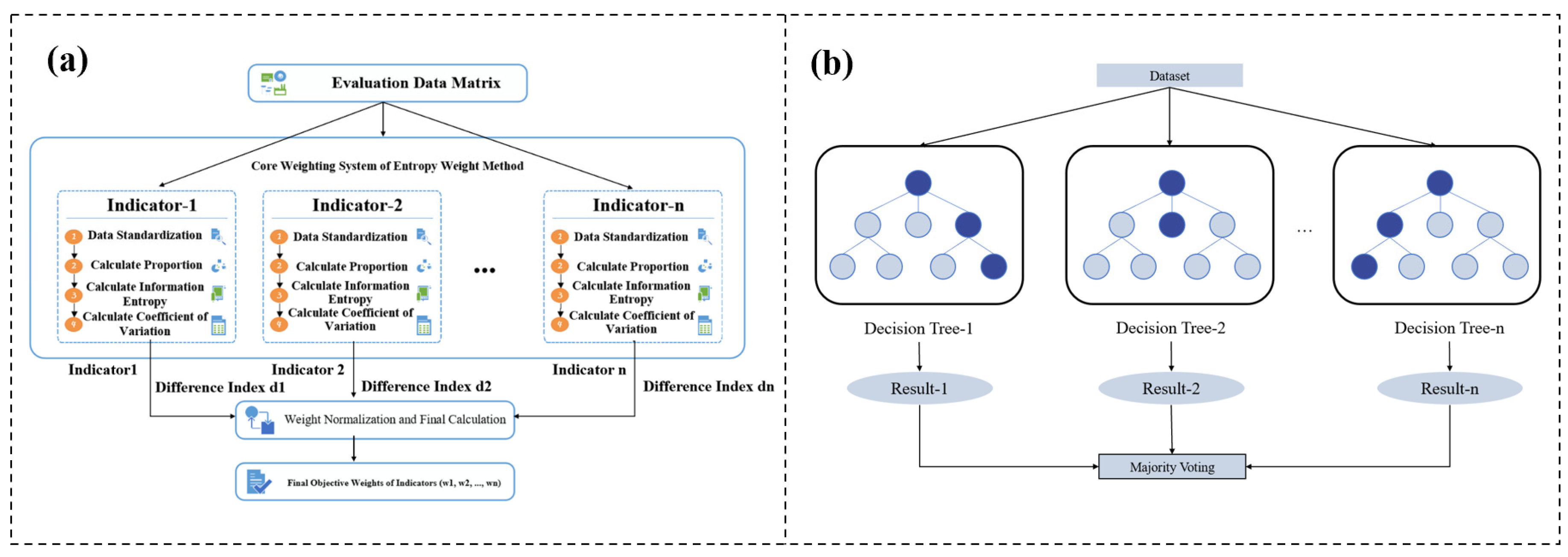
Random Forest (RF) is an ensemble learning algorithm predicated on the bootstrap aggregating (bagging) strategy, which enhances predictive performance by constructing a multitude of independent decision trees in parallel. Each tree is trained on distinct bootstrap samples and randomized feature subsets, with the final outputs aggregated—typically through majority voting for classification or averaging for regression—to ensure numerical stability. This dual-randomness mechanism effectively mitigates overfitting, thereby endowing the model with robust generalization capability and noise resilience.

Parallel to this, the EWM is employed as an objective weighting technique derived from the concept of entropy in information theory. It determines the relative importance of indicators by quantifying their degree of informational variation. Specifically, indicators characterized by higher data variability and lower entropy values are identified as carrying more significant information and are consequently assigned greater weights. Conversely, indicators with higher homogeneity and entropy receive lower weights. By relying solely on the intrinsic dispersion of raw data, the EWM eliminates subjective bias, ensuring a rigorous and data-driven weighting process. The operational flowchart of the EWM is schematically illustrated in Figure 1.

2.1.1. RF

RF is an ensemble learning approach that implements prediction by constructing multiple decision trees and aggregating their output results [29]. Its core principle relies on two types of randomness. The first is data randomness: several distinct subsets are randomly sampled from the original dataset using the bootstrap sampling method. The second resides in feature randomness: at each node split, each tree only adopts a randomly selected feature subset instead of the entire available feature set. In random forests, Feature Importance Analysis is performed by evaluating the reduction in impurity caused by each feature during node splitting. Assume that feature $X_j$ is employed to split the samples at node $t$ Let the impurity of node $t$ before splitting be $I\left(t\right)$, the impurities of the left and right child nodes be $I\left(t_L\right)$ and $I\left(t_R\right)$ respectively, and the corresponding sample proportions be $p_L$ and $p_R$. Then the contribution of feature $X_j$ can be expressed as:

$$\begin{array}{c}∆I\left(t\right)=I\left(t\right)-p_{L}I\left(t_L\right)-p_{R}I\left(t_R\right)\end{array}$$

(1)

For each decision tree, the impurity reduction associated with each feature across all splitting nodes is computed individually [27]. The global feature importance is derived by accumulating and averaging these contribution scores.

2.1.2. Entropy Weight Method

To avoid the bias caused by subjective weighting and objectively identify the key factors influencing oil rate, the Entropy Weight Method is introduced in this paper. Firstly, the n evaluation indicators corresponding to m evaluation objects are arranged into an original data matrix in a specified order, where l ≤ i ≤ m and 1 ≤ j ≤ n.

$$\begin{array}{c}X={\left(x_{ij}\right)}_{m\times n}\end{array}$$

(2)

where $x_{ij}$ denotes the value of the j-th indicator for the i-th sample.

Secondly, the original data were standardized using the Min-Max normalization to eliminate dimensional effects. Given the differences in dimensions and magnitudes among evaluation indicators, direct calculation may lead to distorted results. Therefore, standardization was performed to remove dimensional influences and map all indicator values into the range [0, 1]. Positive indicators are defined as those for which a higher value represents a better evaluation effect, whereas negative indicators are those for which a lower value represents a better evaluation effect. The corresponding calculation formulas are given as follows.

Positive indicators:

$$\begin{array}{c}{x}_{ij}^{+}={\displaystyle \frac{x_{ij}-\mathit{min}\{x_{ij}\}}{\mathit{max}\{x_{ij}\}-\mathit{min}\{x_{ij}\}}}\end{array}$$

(3)

Negative indicators:

$$\begin{array}{c}{x}_{ij}^{-}={\displaystyle \frac{\mathit{max}\{x_{ij}\}-x_{ij}}{\mathit{max}\{x_{ij}\}-\mathit{min}\{x_{ij}\}}}\end{array}$$

(4)

where $\mathit{max}\{x_{ij}\}$ and $\mathit{min}\{x_{ij}\}$ represent the maximum and minimum values of the j-th indicator across all samples, respectively.

Third, coordinate translation was performed on the standardized positive and negative indicators. Since the standardized values obtained by the Min-Max normalization may contain zeros, direct use in subsequent entropy calculation would lead to interruption due to the undefined logarithm of zero. To avoid undefined logarithmic operations, a small epsilon (ε) is added to the normalized data. The translation formulas are given as follows.

Positive indicators:

$$\begin{array}{c}{x}_{ij}^{\prime }={\displaystyle \frac{x_{ij}-\mathit{min}\{x_{ij}\}}{\mathit{max}\{x_{ij}\}-\mathit{min}\{x_{ij}\}}}+\mathrm{\epsilon }\end{array}$$

(5)

Negative indicators:

$$\begin{array}{c}{x}_{ij}^{\prime }={\displaystyle \frac{\mathit{max}\{x_{ij}\}-x_{ij}}{\mathit{max}\{x_{ij}\}-\mathit{min}\{x_{ij}\}}}+\mathrm{\epsilon }\end{array}$$

(6)

where $x_{ij}^{\prime }$ denotes the indicator value after coordinate translation, $\mathrm{\epsilon }=0.0001$.

Fourthly, the proportion of each evaluation object corresponding to each indicator was calculated. Based on the translated indicator values, the proportion of the i-th evaluation object in the j-th indicator was determined to normalize the data, which provides a basis for the subsequent entropy evaluation. The corresponding formula is presented as follows.

$$\begin{array}{c}{p}_{ij}={\displaystyle \frac{x_{ij}^{\prime }}{{\sum }_{i=1}^m{x}_{ij}^{\prime }}}\end{array}$$

(7)

where $p_{ij}$ denotes the proportion of the i-th sample in the j-th indicator, and ${\sum }_{i=1}^m{x}_{ij}^{\prime }$.

Fifthly, the information entropy of each evaluation indicator was calculated. Information entropy is a quantitative index reflecting the disorder degree of data. According to the proportion of each indicator, the information entropy of each indicator was obtained using the entropy formula, where $k$ is the entropy coefficient related to the number of evaluation objects, used to normalize the entropy values into the interval [0, 1]. The corresponding formula is provided as follows.

$$\begin{array}{c}{e}_j=-k{\displaystyle \sum _{i=1}^m}\left(p_{ij}\cdot \ln p_{ij}\right), k={\displaystyle \frac{1}{\ln m}}\end{array}$$

(8)

where $e_j$ denotes the information entropy of the j-th indicator, and 0 ≤ $e_j$ ≤ 1.

Sixthly, the differentiation coefficient of each evaluation indicator was calculated. The differentiation coefficient represents the discrimination ability of the indicator, which is obtained by subtracting the information entropy from 1. A smaller information entropy corresponds to a larger differentiation coefficient, indicating stronger discrimination ability and more effective information contained in the indicator. The corresponding formula is presented as follows.

$$\begin{array}{c}{g}_j=1-e_j\end{array}$$

(9)

where $g_j$ denotes the differentiation coefficient of the j-th indicator.

Seventhly, the differentiation coefficients were normalized to calculate the objective weight of each evaluation indicator. The differentiation coefficients were summed and normalized to ensure the sum of all indicator weights was equal to 1, thereby obtaining the final objective weight of each indicator. A larger weight indicates a more significant influence of the indicator on the research objective. The corresponding formula is provided as follows.

$$\begin{array}{c}{w}_j={\displaystyle \frac{g_j}{{\sum }_{j=1}^n{g}_j}}\end{array}$$

(10)

where $w_j$ denotes the objective weight of the j-th indicator.

Eighthly, the comprehensive score of each evaluation object was calculated. Based on the objective indicator weights $w_j$ and the standardized indicator values $x_{ij}^{\prime }$ after coordinate translation, the comprehensive evaluation score of each object was obtained via weighted summation, so as to realize the comprehensive quantitative ranking of all evaluation objects. The corresponding formula is presented as follows.

$$\begin{array}{c}{F}_i={\displaystyle \sum _{j=1}^n}{w}_j{x}_{ij}^{\prime }\end{array}$$

(11)

where $F_i$ denotes the comprehensive score of the i-th sample.

In summary, the entropy weight method avoids the interference of subjective factors on indicator weighting through objective calculation. Its results can truly reflect the actual contribution of each indicator in the research system, providing an objective and reliable quantitative basis for identifying the key factors affecting oil rate.

2.2. Proxy Model Method

In this study, the prediction accuracy and robustness of the model are verified using various error evaluation metrics, including the mean absolute error (MAE), root mean square error (RMSE), and coefficient of determination (R²). The specific modeling procedure and underlying principle are described as follows.

The modeling process of the standardized surrogate model consists of six core steps: data preparation, feature standardization, model construction, model training, model evaluation, and prediction interpretation. Throughout the process, parameters involved in various stages of CCCP are investigated. High-weight features screened by the EWM and Spearman correlation analysis are adopted as model inputs, ensuring that the model achieves both satisfactory data-fitting performance and physical interpretability [33,34].

2.2.1. Data Preparation

Data preparation serves as the foundation for modeling, which mainly focuses on data quality control and dataset partitioning based on the preprocessed data. The detailed procedures are as follows:

(1) Data collection: The independent variable matrix X with n samples and m features (core production indicators after relative change transformation and physical filtering) and the corresponding continuous dependent variable vector y were organized.

(2) Data cleaning: Missing values were handled using interpolation, and outliers were detected and removed based on the 3σ criterion, so as to ensure data integrity and validity.

(3) Dataset partitioning: The dataset was randomly divided into training sets and test sets at a ratio of 80%:20%. The training set was used for model parameter fitting, while the test set was adopted to verify the generalization ability of the model.

2.2.2. Feature Standardization

The MLR is sensitive to the dimension and magnitude of features. Features with large numerical differences tend to dominate model parameter fitting, resulting in slow convergence of gradient descent and increased model bias. Standard Scaler transforms each feature into a standard distribution with a mean of 0 and standard deviation of 1 via mean-std normalization. It eliminates dimensional differences while preserving the original distribution of features. The detailed procedure is as follows.

(1) A StandardScaler object was constructed.

The mean ${\mu }_j$ and standard deviation ${\sigma }_j$ of each feature j were calculated based on the training dataset.

$$\begin{array}{c}{\mu }_j={\displaystyle \frac{1}{n_{\mathrm{train}}}}{\displaystyle \sum _{i=1}^{n_{\mathrm{train}}}}{x}_{ij},{\sigma }_j=\sqrt{{\displaystyle \frac{1}{n_{\mathrm{train}}}}{\displaystyle \sum _{i=1}^{n_{\mathrm{train}}}}(x_{ij}-{\mu }_j{)}^2}\end{array}$$

(12)

where, $n_{\mathrm{train}}$ is the number of samples in the training set, and $x_{ij}$ is the value of the j-th feature for the i-th sample in the training set.

(2) The features of the training set were standardized using ${\mu }_j$ and ${\sigma }_j$ obtained from the training set,

$$\begin{array}{c}{x}_{ij}^{\mathrm{train},\mathrm{std}}={\displaystyle \frac{x_{ij}^{\mathrm{train}}-{\mu }_j}{{\sigma }_j}}\end{array}$$

(13)

(3) The features of the test set were standardized using the same set of ${\mu }_j$ and ${\sigma }_j$ derived from the training set, which avoids data leakage from the test set and ensures the objectivity of model validation.

$$\begin{array}{c}{x}_{ij}^{\mathrm{test},\mathrm{std}}={\displaystyle \frac{x_{ij}^{\mathrm{test}}-{\mu }_j}{{\sigma }_j}}\end{array}$$

(14)

2.2.3. Model Construction

Although the base MLR model is linear, nonlinear relationships are implicitly captured through feature weighting, data transformation, and the nonlinear characteristics embedded in the CMG-generated training dataset. In this study, the MLR was mainly employed to establish a linear relationship between standardized input features and predicted oil rate. A nonlinear expansion interface was reserved to form a model architecture dominated by single-layer linear mapping and assisted by multi-layer nonlinear mapping. The specific forms are as follows:

(1) MLR

As the basic form of the model, a linear combination relationship between input features and output was directly constructed, as expressed by

$$\begin{array}{c}\hat{y}=X^{std}\cdot w+b\end{array}$$

(15)

where $\hat{y}$ is the predicted oil rate, $X^{std}$ is the standardized input feature matrix, $w$ is the feature weight vector, and $b$ is the bias term of the model.

(2) Neural network regression

The MLR was constructed for samples with significant local nonlinearity. The model consists of an input layer with m nodes, several hidden layers using the ReLU activation function for nonlinear transformation, and an output layer with one linear node for predicting oil rate. The expression is given as follows,

$$\begin{array}{c}\hat{y}=f\left(w_n\left(X^{std}\right);\theta \right)\end{array}$$

(16)

where $f\left(X\right)$ is the nonlinear mapping function of the network, $w_n$ denotes the weights of each layer, and $\theta$ represents all trainable parameters of the network.

2.2.4. Model Training

The model was trained using the MSE as the loss function. The gradient descent method was adopted to iteratively optimize the model parameters until the loss function converged to a stable value. The core loss function is given by

$$\begin{array}{c}L={\displaystyle \frac{1}{n_{\mathrm{train}}}}{\displaystyle \sum _{i=1}^{n_{\mathrm{train}}}}({\widehat{y}}_i-y_i{)}^2\end{array}$$

(17)

where $y_i$ is the measured oil rate of the i-th sample, and ${\widehat{y}}_i$ is the predicted oil rate of the i-th sample. Features standardized by StandardScaler can accelerate the convergence of gradient descent, and effectively avoid parameter oscillation caused by feature scale differences or local optima during model training.

2.2.5. Model Evaluation

Model evaluation was performed based on the standardized test set. The standardized test set features $X_{test}^{std}$ were input into the trained model to obtain the predicted oil rate ${\widehat{y}}_{test}$. By comparing ${\widehat{y}}_{test}$ with the measured values $y_{test}$, several regression metrics were calculated to comprehensively quantify the prediction accuracy and robustness of the model. The key evaluation indices are as follows.

(1) MSE reflects the mean squared deviation between predicted and measured values; a smaller value indicates higher fitting accuracy.

(2) RMSE obtained by taking the square root of MSE, which recovers the original data dimension and directly reflects the prediction error.

(3) MAE reflects the mean absolute deviation between predicted and measured values, with stronger robustness to outliers.

(4) R² indicates the ability of the model to explain data variation; a value closer to 1 represents better fitting performance.

2.2.6. Model Prediction

When predicting oil rate for samples using the trained model, the same preprocessing workflow as the training set was strictly followed to ensure valid predictions. The procedure is as follows:

(1) Standardization: Preprocessed features of new samples were standardized using the StandardScaler fitted during model training (μ_j and σ_j) from the training set.

(2) Model prediction: The standardized features were input into the trained regression model to directly obtain the predicted oil rate ${\widehat{y}}_{new}$.

(3) Model interpretation: The magnitude and sign of the feature weight vector ω were analyzed to quantify the influence of each production indicator on oil rate. A positive weight indicates that an increase in the indicator promotes oil rate, while a negative weight suggests the opposite. A larger absolute weight corresponds to a more significant effect.

2.3. Reservoir Numerical Simulation Methods

To gain an in-depth analysis of the production dynamic evolution characteristics of chemical composite cold production from the perspective of reservoir engineering, and to verify the data-driven results of feature importance analysis and surrogate models from the physical mechanism level, a numerical model for the heavy oil reservoir in Well Block Z is established using reservoir numerical simulation. This method simulates the multiphase flow of oil and water in the reservoir and wellbore, revealing the intrinsic relationship among water cut rise, flow regime transition, and oil production fluctuation. The numerical simulation is carried out with the CMG (Computer Modelling Group Ltd., Calgary, AB, Canada) 2022 software, and the STARS module is adopted to model the displacement process of chemical composite cold production, which can accurately characterize the rheological properties of the fluid and the multiphase flow behavior of heavy oil.

2.3.1. Mathematical Model

Characterizing the two-phase flow process of oil and water in heavy oil reservoirs is the core of establishing a mathematical model for CCCP. Combining Darcy’s law with mass conservation equations, this study establishes a reservoir flow mathematical model suitable for chemical composite cold production calibrated against 5 sets of core experimental measurements covering oil/water phase relative permeability and viscosity parameters (covering the observed values of core parameters of oil and water phases) [35]. This model can comprehensively characterize the fluid flow dynamics in the reservoir during the chemical composite cold production process and accurately reflect the impact of cold production measures on the seepage characteristics of reservoir fluids and the variation law of oil production. The model consists of four parts: governing equations, auxiliary equations, initial conditions, and boundary conditions, which are detailed as follows.

(1) Governing Equations

As the core of the mathematical model, the governing equations are established based on the law of mass conservation. Combined with the observation rules of the 5 data points, they describe the mass change characteristics of oil and water phases during the reservoir seepage process, ensuring that the equations are consistent with the actual observed data and conform to the actual engineering scenario of chemical composite cold production.

Oil-phase mass conservation equation:

$$\begin{array}{c}{\displaystyle \frac{\partial \left(\varnothing {\rho }_o{S}_o\right)}{\partial t}}+\nabla ·\left({\rho }_o{v}_o\right)=q_o\end{array}$$

(18)

where $\varnothing$ is porosity, ${\rho }_o$ is oil phase density, $S_o$ is oil saturation, $v_o$ is oil phase velocity, and $q_o$ is the oil phase source/sink term.

Water phase mass conservation equation

$$\begin{array}{c}{\displaystyle \frac{\partial \left(\varnothing {\rho }_w{S}_w\right)}{\partial t}}+\nabla ·\left({\rho }_w{v}_w\right)=q_w\end{array}$$

(19)

where ${\rho }_w$ is water density, $S_w$ is water saturation, $v_w$ is water phase velocity vector, and $q_w$ is the water phase source/sink term.

(2) Auxiliary Equations

The flow velocities of the oil and water phases follow Darcy’s law. Combined with the observed values of seepage parameters from the 5 data points, the rationality of the equation parameters is ensured, which is consistent with the seepage law of chemical composite cold production.

$$\begin{array}{c}{v}_o=-{\displaystyle \frac{{kk}_{ro}}{{\mu }_o}}\left(\nabla p_o-{\rho }_{o}g\nabla z\right)\end{array}$$

(20)

$$\begin{array}{c}{v}_w=-{\displaystyle \frac{{kk}_{rw}}{{\mu }_w}}\left(\nabla p_w-{\rho }_{w}g\nabla z\right)\end{array}$$

(21)

where $k_{ro}$ and $k_{rw}$ are the relative permeabilities of the oil and water phases, ${\mu }_o$ and ${\mu }_w$ represent the viscosities of the oil and water phases. Notably, ${\mu }_w$ is dependent on the concentration, as detailed in Equation (21). $K$ is the absolute permeability tensor, $p_o$ and $p_w$ are the oil and water pressures, $g$ is gravitational acceleration, and $z$ is the vertical coordinate.

A power-law empirical model is adopted to characterize the influence of relevant factors on water phase viscosity during the chemical composite cold production. The model parameters are fitted based on the observed values of water phase viscosity and relevant influencing parameters from the 5 data points, and the expression is as follows,

$$\begin{array}{c}{\mu }_w={\mu }_{w0}\left(1+\alpha C_p^{\beta }\right)\end{array}$$

(22)

where ${\mu }_{w0}$ is the viscosity of pure water, $\alpha$ and $\beta$ are empirical fitting parameters used to characterize the viscosity enhancement effect induced by concentration.

Assuming two-phase flow of oil and water without gas participation, consistent with the actual cold production scenario,

$$\begin{array}{c}{S}_o+S_w=1\end{array}$$

(23)

The difference between the water phase pressure and the oil phase pressure is known as the capillary pressure, or $p_c$,

$$\begin{array}{c}{p}_c=p_o-p_w\end{array}$$

(24)

(3) Initial Conditions

Based on the initial observed parameters of the 5 data points and combined with the actual initial state of the reservoir, the initial conditions of the model are determined to ensure that the initial state of the model is consistent with the actual reservoir.

$$\begin{array}{c}{S}_w\left(x,y,z,t=0\right)=S_w^0\end{array}$$

(25)

$$\begin{array}{c}{C}_p\left(x,y,z,t=0\right)=C_p^0\end{array}$$

(26)

$$\begin{array}{c}p\left(x,y,z,t=0\right)=p^0\end{array}$$

(27)

(4) Boundary Conditions

Combined with the actual development method of chemical composite cold production, referring to the observed values of boundary parameters from the 5 data points, the boundary conditions of the model are set to ensure that the model is consistent with the on-site engineering practice:

Pressure Boundary Conditions

$$\begin{array}{c}p\left(x,y,z\right)=p_{inj}\end{array}$$

(28)

$$\begin{array}{c}p\left(x,y,z\right)=p_{prod}\end{array}$$

(29)

where $p_{inj}$ is the injection well pressure, $p_{prod}$ is the production well pressure (determined based on the well pressure observed values of the 5 data points).

Flux Boundary Conditions

$$\begin{array}{c}{v}_w·n=v_{inj}\end{array}$$

(30)

where $v_{inj}$ is the injection rate (calibrated by the observed values of injection parameters from the 5 data points), and $v_w$ is the boundary normal vector.

Closed Boundary Condition

$$\begin{array}{c}{v}_0·n=0\end{array}$$

(31)

$$\begin{array}{c}{v}_w·n=0\end{array}$$

(32)

2.3.2. Establishment of the Numerical Model

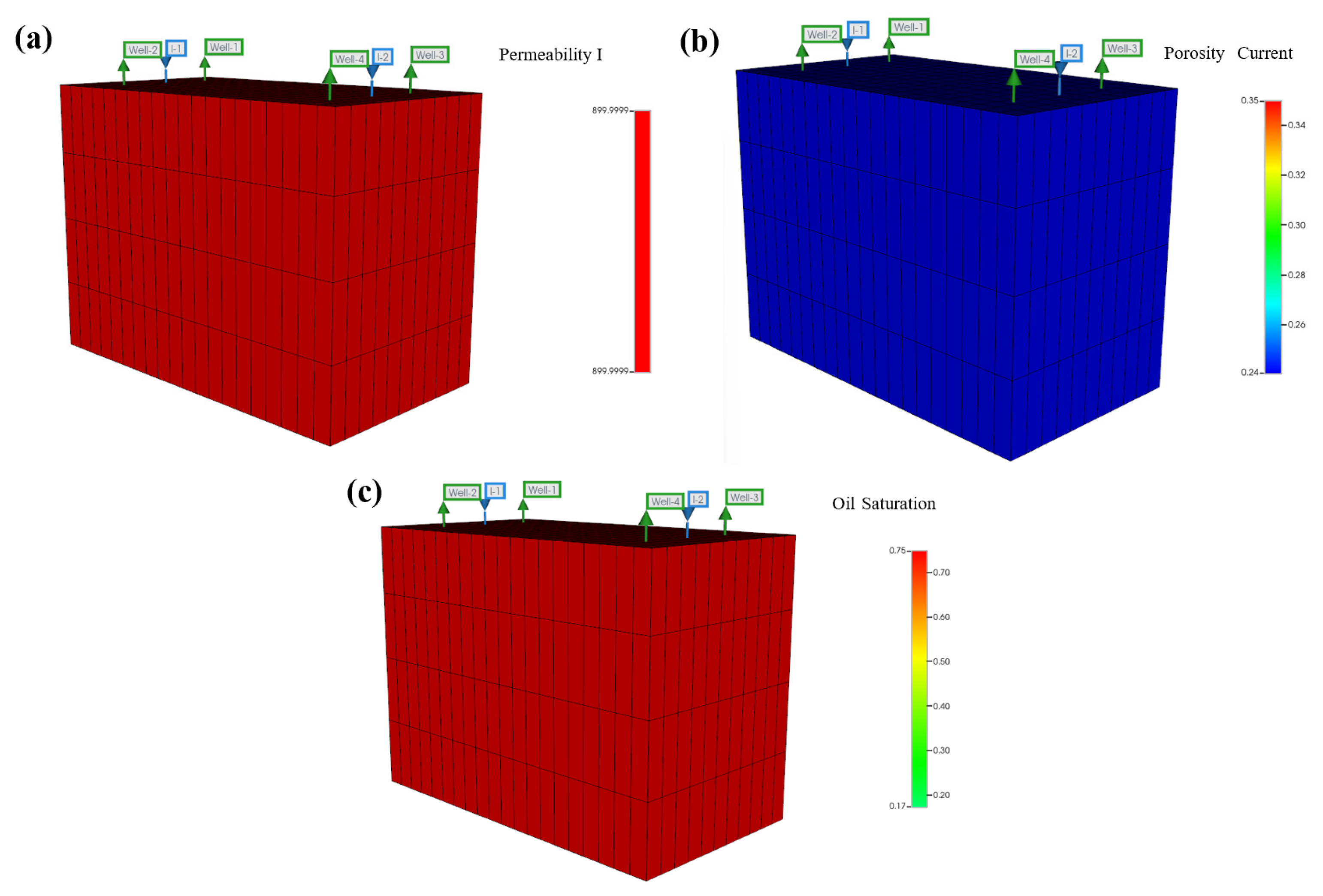
The CMG numerical simulation program is used in this study to create a conceptual model with a total grid number of 880 (i × j × k = 20 × 11 × 4), where the grid division is optimized according to the actual geological structure and production well distribution of the Z well area, with fine grid encryption in the near-well zone to accurately characterize the fluid seepage law in the high-permeability zone and the rapid change in production parameters near the wellbore. The specific model setup is displayed in Figure 2, including the permeability distribution model, porosity distribution model and initial oil saturation distribution model, which are all calibrated based on the actual core test data and logging interpretation results of the Z well area to ensure the geological consistency of the numerical model.

The key reservoir and fluid parameters of the numerical model are set based on the field-measured data and core experiment results, with the specific settings as follows: the reservoir burial depth is in the range of 750 m to 758 m, the average absolute permeability of the reservoir is 900 mD, the initial oil saturation is 75%, the crude oil viscosity is 450 mPa·s under reservoir conditions, the porosity is 24%, and the reservoir temperature is a constant value of 75 °C consistent with the actual formation temperature. The solution used in chemical composite cold production adopts a power-law non-Newtonian fluid model, and its viscosity change law is characterized by the water phase viscosity model in Equation (22), with the empirical fitting parameters α and β determined by core flooding experiments.

The STARS module of the CMG numerical simulation software was selected to simulate the displacement process of the heavy oil reservoir under chemical composite cold production. This module is equipped with a sophisticated mathematical model, which can accurately characterize the rheological properties of the working fluid (e.g., shear-thinning effect) and the multiphase flow behaviors of heavy oil in porous media. Furthermore, it can effectively simulate the adsorption, retention, and diffusion of chemical agents in the reservoir, as well as the changes in the relative permeability curve induced by these agents.

The production development history of the numerical model is set to be consistent with the actual development process of the Z well area: the model started production in 2006, and the initial waterflooding development phase lasted for 6 years. During this period, the formation energy was supplemented by water injection, and the basic production pattern of the reservoir was established. With the steady decrease in waterflooding development efficiency and the continuous rise of water cut to more than 80% in 2011, the development approach was officially shifted to chemical composite cold production, and the numerical simulation was continuously carried out until 2025, covering the full cycle of chemical composite cold production development of the reservoir for 14 years.

In the stage of the model, the injection parameters are set according to the field construction scheme: the initial injection concentration is 4000 mg/L, the injection rate is 236 m³/d, and the injection mode is continuous slug injection to ensure the stable propagation of the solution in the reservoir and form an effective displacement front. The production well adopts the fixed liquid production rate production mode, which is consistent with the actual production control mode of the Z well area, and the production pressure is dynamically adjusted according to the reservoir pressure change to maintain the stable production of the oil well.

Based on long-term numerical simulations over the full development cycle, the reservoir performance of Well Block Z under CCCP is quantitatively evaluated. By 2025, the comprehensive water cut of the reservoir reached 98.6%, which is in good agreement with field monitoring data, reflecting the inherent trend of rising water cut in the late stage of heavy oil development. The cumulative oil production amounted to 249,008 m³, with a final oil recovery factor of 43%—an increase of more than 10 percentage points compared with the conventional waterflooding stage. This fully validates the technical effectiveness of chemical composite cold production in enhancing heavy oil recovery.

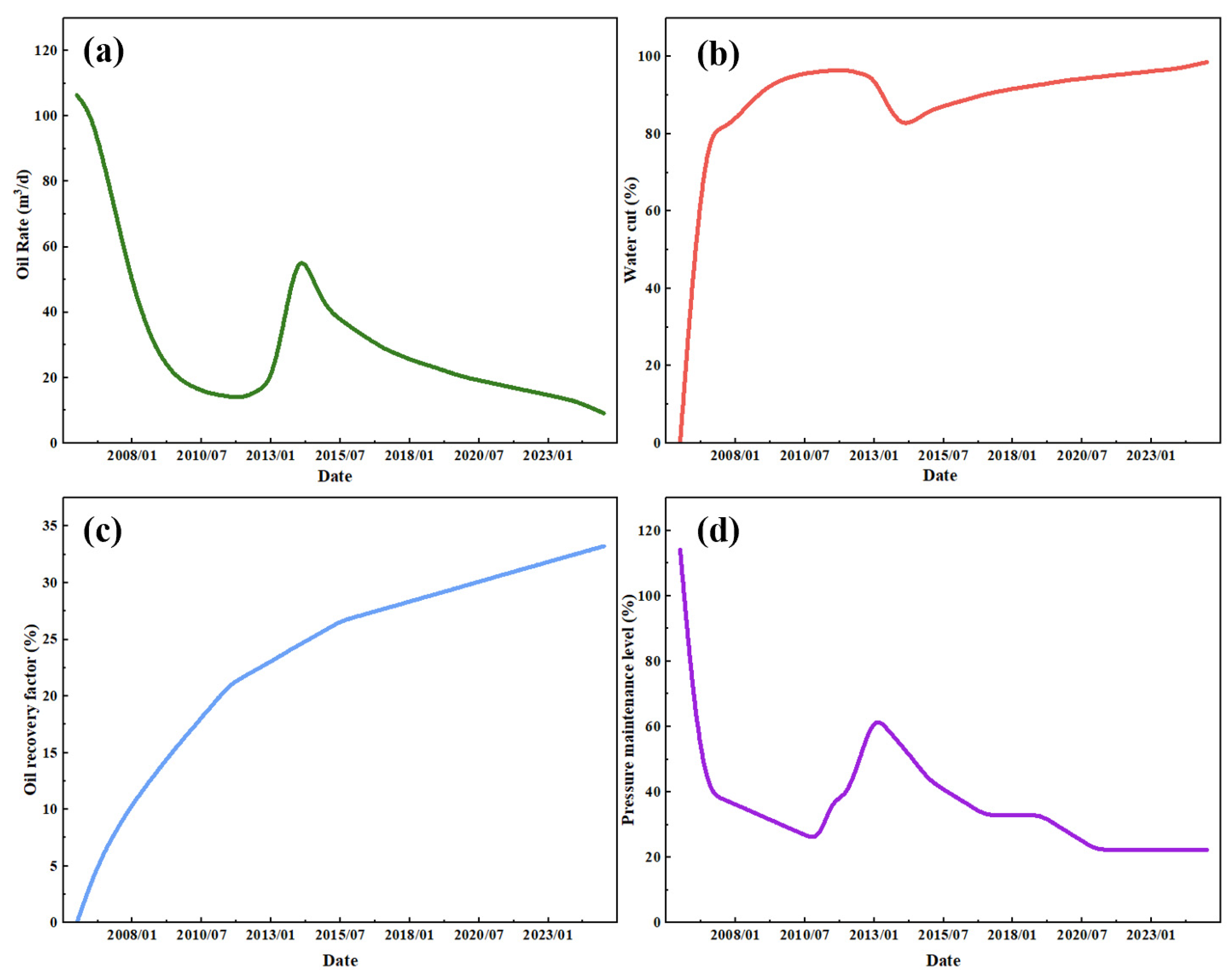
Figure 3 presents the key production performance curves of the model, including oil production rate, water cut, oil recovery factor, and reservoir pressure maintenance level. These curves comprehensively illustrate the dynamic evolution characteristics of the reservoir throughout the entire development process from waterflooding to chemical composite cold production.

2.3.3. Model Matching

To ensure the numerical model can accurately reflect the actual production dynamic characteristics of the Z well area and provide a reliable physical mechanism basis for the subsequent data-driven Feature Importance Analysis and production prediction, a history matching process was carried out for the established numerical model, with the field-measured production data of the Z well area from 2006 to 2025 as the fitting benchmark. The core goal of history matching is to minimize the objective function of the sum of squared errors between the model’s predicted values and field observed values for key production parameters, and continuously optimize the model’s core parameters through multiple iterative adjustments to achieve a high degree of consistency between the simulation results and the actual field data.

In the history matching process, the parameters were set in accordance with the actual field construction scheme: injection was officially initiated in 2011 with an initial injection concentration of 4000 mg/L and a constant injection rate of 236 m³/d; the production wells adopted the field-based liquid production control mode, and the model’s boundary conditions and production system were kept consistent with the on-site engineering practice.

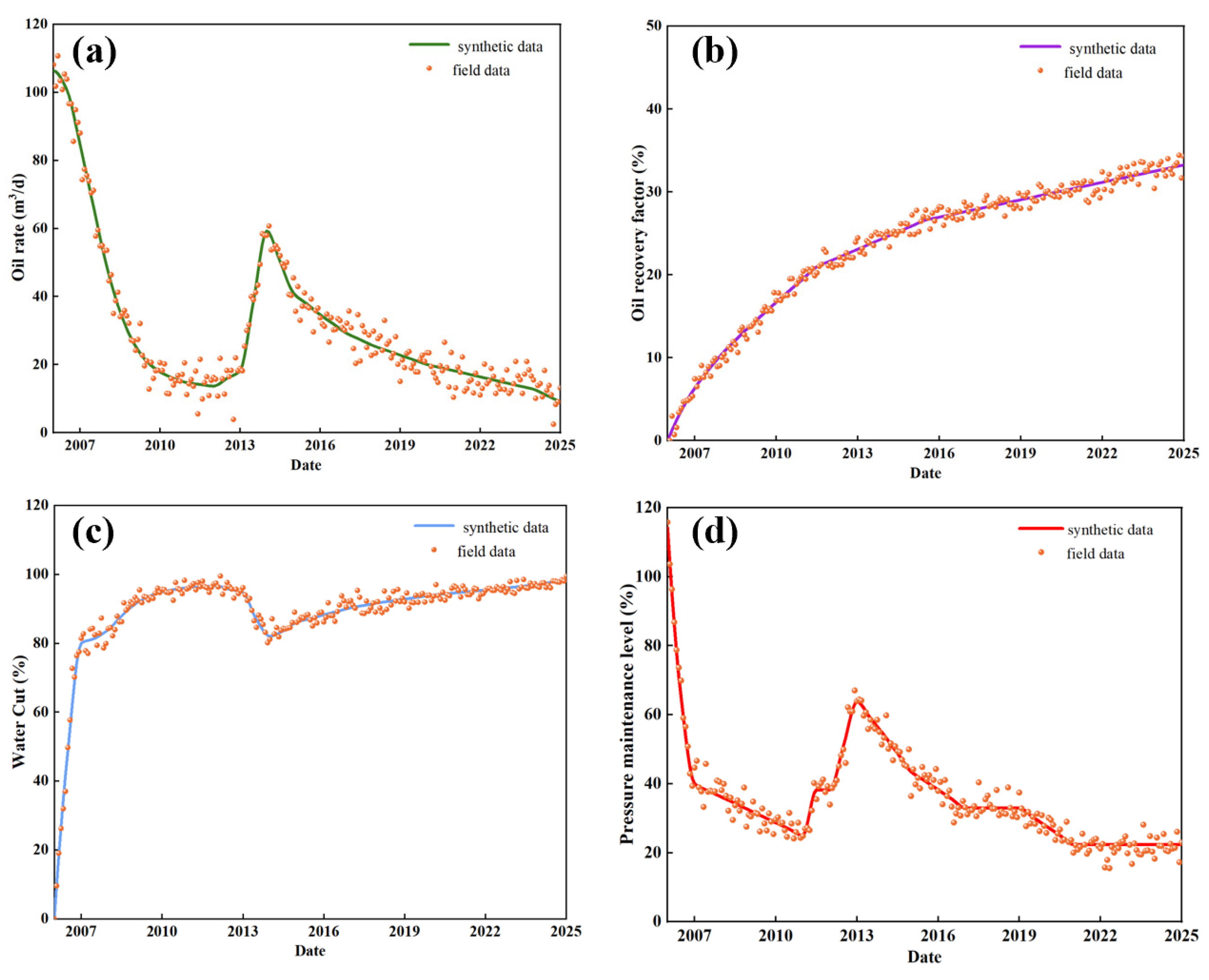
After several rounds of parameter calibration and iterative optimization, the numerical model achieved an excellent fitting effect with the field-measured data, and the overall relative deviation of the core production parameters was controlled within 10%, which fully demonstrated the model’s ability to faithfully replicate the actual dynamic evolution characteristics of the Z well area reservoir. As shown in Figure 4, the model’s predicted values and field observed values of four key evaluation indicators show an almost overlapping trend with time, reflecting the high accuracy and reliability of the numerical model:

The model can accurately characterize the evolution law of the oil rate of the reservoir throughout the transition from water flooding development to chemical composite cold production, and realize high-precision simulation of the slow decline characteristic of oil rate in the water flooding stage and the variation trend of the reservoir’s stable production stage after switching to Figure 4a. The predicted values of oil rate in the full time series are highly consistent with the field-measured values, with no significant systematic deviations observed. For the water cut index, the simulation curve truly reproduces its actual evolution characteristics in reservoir development: the water cut rises slowly in the early stage of water flooding development, surges rapidly in the middle and late stages, and the rising rate of water cut slows down significantly after the implementation of Figure 4b. The model predicts that the water cut will reach 98.6% by 2025, aligning closely with field monitoring data and validating the model’s capacity to characterize flow regime changes induced by chemical agents. The oil recovery factor grows at a low rate in the water flooding stage, and an obvious inflection point appears in the oil recovery factor curve after switching to chemical composite cold production with the growth entering an accelerated phase. The final model-predicted oil recovery factor reaches 43%, which aligns closely with the actual field development results Figure 4c, thereby confirming the model’s capability to accurately characterize CCCP displacement efficiency. Furthermore, the reservoir pressure maintenance level predicted by the model matches the field-measured data with high fidelity. The model accurately captures the dynamic fluctuations in reservoir pressure under the synergistic effects of water injection and CCCP fluids, effectively reflecting the impact of the on-site injection-production system on formation energy conservation (Figure 4d). This alignment is critical to ensuring the model’s precision in characterizing fluid seepage mechanisms and the evolution of production dynamics. In summary, the numerical model validated by history matching is highly consistent with the actual geological and production characteristics of the Z well block, and can accurately characterize the seepage dynamics of oil-water in the reservoir, the flow pattern transition law induced by water cut rise, and the production dynamic evolution characteristics throughout the chemical composite cold production process. On the one hand, the model verifies the rationality of the constructed mathematical model for chemical composite cold production from the perspective of numerical simulation; on the other hand, it provides a solid physical mechanism support for the subsequent data-driven Feature Importance Analysis of production parameters and the construction of machine learning prediction models, and also lays an important foundation for the in-depth analysis of the intrinsic mechanism of oil rate during the chemical composite cold production process.

3. Feature Importance Analysis

3.1. Feature Symbol Definition

To standardize the quantitative analysis of production dynamic parameters and unify the input variables of the subsequent machine learning model, the core physical and production parameters involved in the Feature Importance Analysis and prediction of chemical composite cold production in the Z well block are defined with unified symbols. All parameters are referred to by their corresponding symbols in the subsequent calculation, modeling and analysis processes to ensure the consistency and readability of the research process. The specific correspondence between parameters and symbols is shown in

Table 1. Parameters.

Parameters	Symbol
Temperature	T
Injection concentration	Ci
Injection Rate	Qi
Injection-production balance and development	Qp
Maximum Adsorption Capacity	Admaxt

.

3.2. Factors Correlation

Based on the multiphase flow mathematical model established in Section 2.3.1, T, Ci, Qi, Qp and Admaxt were selected as the core independent variables for Feature Importance Analysis, with the selection deeply coupled with the fluid flow dynamics of chemical composite cold production. Each parameter exerts a unique regulatory effect on the production dynamics of heavy oil reservoirs:

Thermodynamic and rheological control (T): As indicated in Equation (13), the viscosity of solution exhibits a high correlation to temperature. Variations in temperature directly alter the rheological properties of formation fluids, thereby influencing the flow resistance in Darcy’s law (Equations (11) and (12)), and thus serving as the fundamental physical condition that determines displacement efficiency. Displacement driving force and sweep control (Ci, Qi): Injection parameters act as the key source terms in the mass conservation equations (Equations (9) and (10)). Ci dictates the magnitude of water-phase viscosity enhancement (Equation (13)), while Qi dominates the evolution of pressure gradients and water cut. Together, they constitute the core energy excitation at the injection end of chemical composite cold production. Interface effect and hysteresis characteristics (Admaxt): In accordance with the Langmuir adsorption model, the maximum adsorption capacity determines the retention and loss of in porous media. This parameter is directly correlated with the effective action cycle of and the breakthrough rate of flow pattern transition. Injection-production balance and development intensity (Qp): As the sink term at the production end, Qp forms the reservoir pressure maintenance system jointly with injection-end parameters. Investigating the fluctuations of Qp enables the revelation of the coupling relationship between fluid production intensity and reservoir pressure evolution.

In the Feature Importance Analysis framework, the above five parameters were treated as mutually independent decision variables. Although extremely weak cross-correlations may exist among various physical properties in the macro thermodynamic system, such weak correlations have a negligible impact on the overall correlation ranking in statistical modeling.

In contrast, oil rate, water cut, pressure maintenance level and oil recovery factor were defined as dependent variables, forming an indicator system for evaluating the dynamic evolution of the reservoir. A clear physical causal relationship exists between the independent and dependent variables: temperature and adsorption characteristics affect fluid flow by modifying fluid properties, while injection and production parameters guide the evolution of pressure and saturation fields through the injection-production balance system. This design logic of physical mechanism-driven and data feature-quantified lays a theoretical foundation for the subsequent objective evaluation of the dominant factors governing oil rate using the EWM.

In summary, the selected independent and dependent variables exhibit a distinct causal relationship and constitute the key factors influencing reservoir production behavior. Quantifying the exact numerical relationships of such causalities enables a more accurate prediction of oil rate.

3.3. Spearman Analysis Results

To further elucidate the interrelationships between input and output variables, the Spearman correlation coefficient, a nonparametric statistical metric for assessing the monotonic association between two variables, was employed to quantify both the mutual independence of input variables and their correlativity with output variables [31,34]. The Spearman correlation coefficient is calculated as follows:

$$\begin{array}{c}{r}_s=1-{\displaystyle \frac{6\sum d_i^2}{n\left(n^2-1\right)}}\end{array}$$

(33)

where $n$ is the sample size and $d_i$ is the rank difference between two variables. Perfect positive monotonic correlation is denoted by $r_s=1$, perfect negative monotonic correlation by $r_s=-1$, and the absence of any monotonic relationship by $r_s=0$.

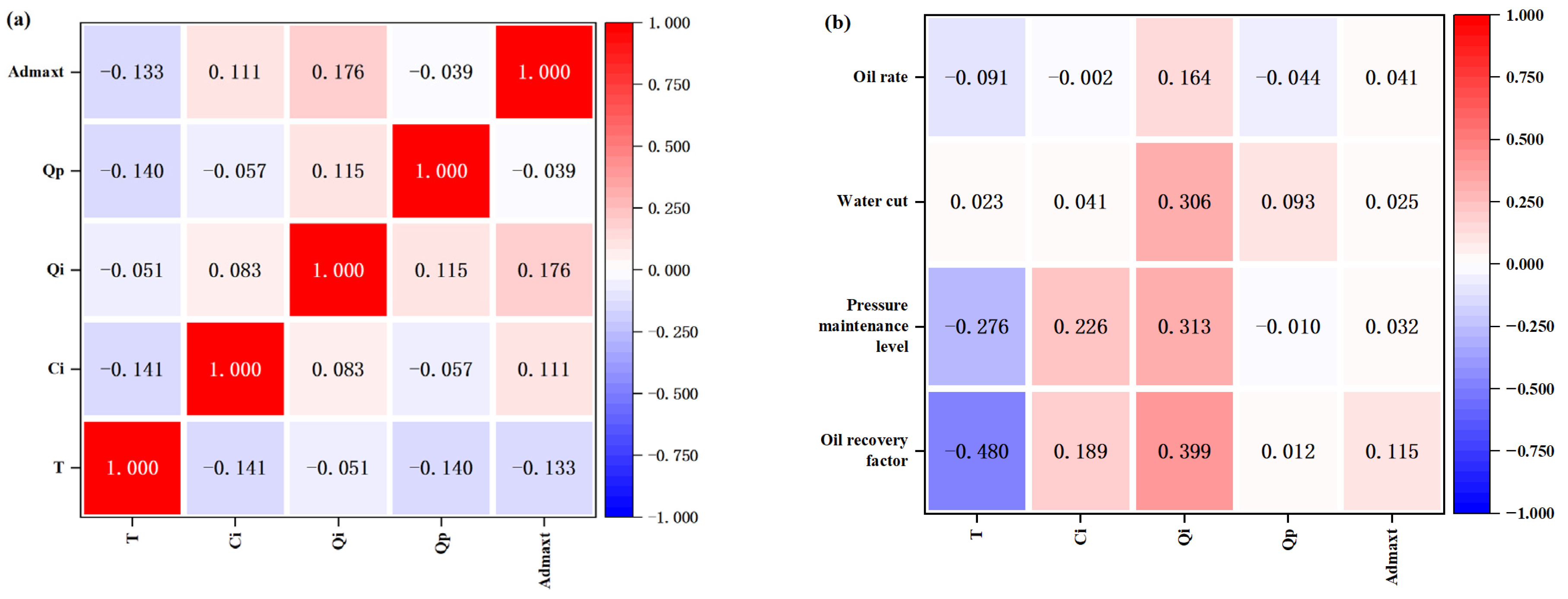
As shown in Figure 5, quantitative analysis of the resulting correlation matrix reveals that all input variables exhibit only weak monotonic associations with one another. In accordance with statistical principles an absolute Spearman correlation coefficient approaching zero indicates a negligible monotonic relationship between variables [25,31]. As visualized in the heatmap, the correlation coefficients among the independent variables are universally close to zero, confirming the absence of significant multicollinearity or strong intercorrelations within the input set. This statistical independence validates the applicability of these variables for subsequent Feature Importance Analysis, as it eliminates the potential adverse impacts of multicollinearity on the stability and interpretability of the analytical model. Additionally, the relatively high Spearman correlation coefficients observed between the independent and dependent variables reflect robust statistical linkages between the core physical parameters and production performance indicators. These significant correlations not only provide a solid theoretical underpinning for the formulation of reservoir development strategies but also enable effective interpretation of the driving factors behind oil production fluctuations in chemical composite cold production.

3.4. EWM Analysis Results

Following the verification of statistical independence among variables, a dual-driven feature engineering framework, integrating the EWM, was implemented to quantitatively evaluate the contribution of each core input variable to the oil production rate. This approach identifies the dominant features governing the production dynamics of chemical composite cold production.

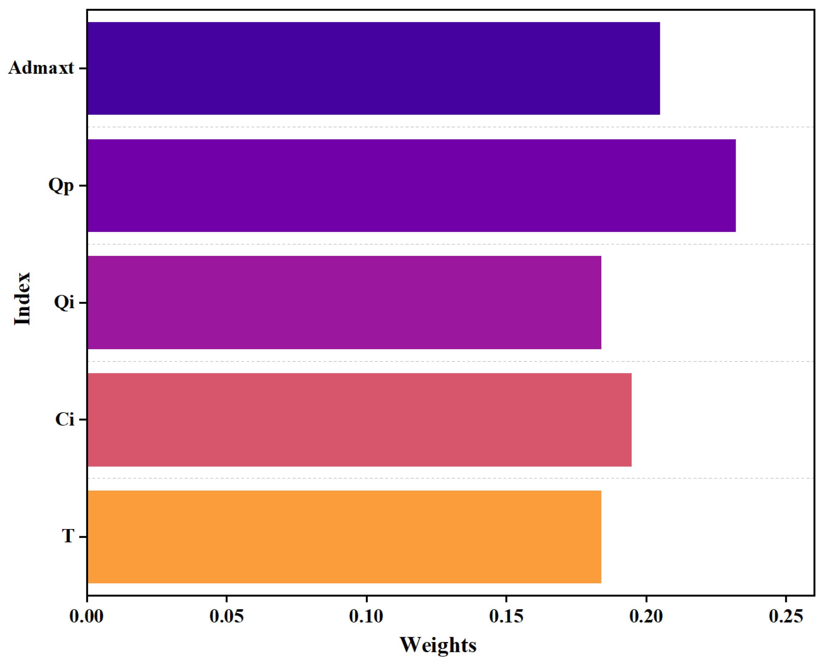
The Spearman correlation heatmap generated by the algorithm (Figure 6) confirmed that the correlation coefficients among the five core input variables (T, Ci, Qi, Qp, Admaxt) were generally close to 0, which verified the statistical independence of physical parameters from the perspective of machine learning and eliminated multicollinearity interference in subsequent model training. On this basis, the EWM was used to calculate the information entropy, objective weight and contribution rate of each parameter to oil rate, with the calculation results presented in

Table 2. Entropy value, objective weight and contribution rate of core parameters.

Parameter	Entropy (ei)	Weight (EWM)	Contribution
T	0.228	0.184	18.40%
Ci	0.181	0.195	19.50%
Qi	0.228	0.184	18.40%
Qp	0.029	0.232	23.20%
Admaxt	0.14	0.205	20.50%

and the weight distribution visualized in the indicator weight histogram.

According to the EWM results (Figure 6), the influence weights of various indicators on production fluctuations are relatively distributed. Specifically, injection-production balance and development (Qp) ranks first with a weight of 23.2%, closely followed by maximum adsorption capacity (Admaxt) at 20.5%. This indicates that in CCCP systems, the intensity of injection-production balance and the retention/adsorption loss of chemical agents within the porous media are the dominant physical factors governing production dynamics. These quantitative findings provide a critical foundation for the subsequent predictive framework: by prioritizing these high-weight features, the model can more accurately capture nonlinear production variations induced by chemical component transport and mass loss, thereby enhancing predictive robustness and precision while minimizing computational dimensionality.

4. Data-Driven Production Dynamics Prediction for CCCP Based on Dual-Driven Feature Engineering

To address the complex nonlinear challenges in predicting the production dynamics of CCCP, this chapter develops an integrated predictive framework coupling feature weighting with an MLR model.

First, a dual-driven Feature Importance Analysis, integrating Spearman rank correlation and the EWM, is conducted to quantify the importance of input features and identify the core controlling factors. Subsequently, to ensure the model captures the full complexity of reservoir behavior, Latin Hypercube Sampling (LHS) is employed to construct a highly representative sample space based on extensive datasets generated via CMG numerical simulations. This is followed by weighted standardization to eliminate dimensional interference. Then, the MLR model is trained to achieve the joint prediction of multiple key production indicators. Finally, the model’s performance is rigorously validated in terms of fitting accuracy (R² > 0.94), reliability, and computational efficiency, providing a robust and high-speed algorithmic solution for real-time production forecasting in heavy oil fields.

4.1. Feature Weighting Strategy Based on Spearman Correlation and Entropy Weight Method

This study refers to the research idea of Zheng [32], holding that high variance is not equivalent to high correlation. In a comprehensive evaluation system, the EWM is used to determine the information weight of indicators, which reflects the discrete degree of data. In contrast, the Spearman correlation coefficient measures the synergistic direction between indicator variation and the overall system trend (positive or negative correlation). The combination of the two methods can simultaneously take into account the “variation characteristics” and “trend correlation characteristics” of indicators, thus providing a more comprehensive evaluation perspective than a single method. It should be noted that Spearman correlation and the EWM capture different aspects of feature importance. Spearman correlation reflects the monotonic relationship between input variables and target outputs, indicating statistical sensitivity. In contrast, EWM evaluates the dispersion of data and quantifies the information content of each feature. Since high variance does not necessarily imply strong correlation with the target variable, the integration of these two methods enables a more comprehensive evaluation by jointly considering statistical relevance and information richness. To address the poor interpretability of traditional black-box models and clarify the influence weight of input parameters on production performance before training, a rigorous a priori evaluation of input features is conducted by combining Spearman’s rank correlation coefficient and EWM. Spearman’s rank correlation coefficient is first used to calculate the nonlinear monotonic correlation between parameters and target production indicators, initially screening sensitive parameters with significant impacts on production performance. For the j-th feature vector and the target variable, a larger absolute value of the Spearman coefficient r_j indicates a more significant influence of the feature on the target variable. To avoid the limitations of a single statistical method and reduce subjective bias, EWM is introduced to measure the information entropy of sample data—parameters with higher data dispersion provide more effective information and are assigned higher objective weights.

The absolute values of Spearman coefficients are normalized to obtain the Spearman subjective weight vector w_s, where the Spearman weight w_sj for the j-th feature is defined as:

$$\begin{array}{c}{w}_{sj}={\displaystyle \frac{\left|r_j\right|}{{\sum }_{k=1}^n\left|r_k\right|}}\end{array}$$

(34)

where n denotes the total number of input features.

A multiplicative synthesis model is adopted to fuse ws with the EWM-derived objective weight vector w_e, comprehensively considering the moedl correlation (dominated by w_s) and information purity (dominated by we) of features to highlight core controlling factors. The final comprehensive weight W_j for the j-th feature is calculated as:

$$\begin{array}{c}{W}_j={\displaystyle \frac{w_{sj}\times w_{ej}}{{\sum }_{k=1}^n\left(w_{sk}\times w_{ek}\right)}}\end{array}$$

(35)

After obtaining the comprehensive weight vector W = [W₁, W₂, …, W_n], it was subjected to a Hadamard Product operation with the standardized original input feature matrix X to generate a weighted feature matrix X_weighted, which serves as the input for the subsequent MLR model:

$$\begin{array}{c}{X}_{weighted}=XW\end{array}$$

(36)

This weighted feature matrix enhances the contribution of core factors while suppressing secondary features, laying a foundation for improving model training efficiency and prediction accuracy.

4.2. Sample Space Construction and Data Preprocessing Based on LHS

After quantifying the comprehensive feature weights, constructing a highly representative and engineering-consistent sample space via CMG numerical simulation becomes the cornerstone for the efficient training of the MLR model. However, raw oilfield production data often exhibit disparate engineering dimensions, which can impede the model’s gradient descent convergence and overall stability.

To address this, this section employs LHS to construct a robust sample set that ensures wide coverage of the parameter space. Subsequently, a data preprocessing workflow is implemented, integrating weighted standardization with a “correlation-guided a priori” strategy. This approach filters and scales the sample data based on the previously identified feature importance, effectively enhancing the information density and quality of the feature matrix while eliminating dimensional interference.

4.2.1. Sample Set Generation Based on LHS

Given the high-dimensional nature of reservoir parameters, LHS is employed rather than traditional random sampling. By implementing stratified, equal-probability division across each parameter dimension, LHS ensures a uniform sample distribution within multi-dimensional physical constraints. This approach enables comprehensive coverage of the parameter space with a manageable number of samples.

To construct a robust dataset for machine learning training, extensive numerical simulation runs were conducted using CMG software. The variation range for each core input parameter was defined as ±30% of the benchmark values—which were previously optimized through meticulous history matching of the numerical model. This range effectively encompasses all feasible production regulation scenarios for the targeted well block under CCCP, as detailed in

Table 3. Benchmark Values and Sampling Variation Ranges of Core Input Parameters.

Parameters	Basic Model	±30%
Temperature (°C)	75	[52.5, 97.5]
Injection concentration (mg/L)	4000	[2800, 5200]
Injection-production balance and development (m3/d)	110	[67, 143]
Injection Rate (m3/d)	236	[165.2, 306.8]
Maximum Adsorption Capacity (gmol/m3)	0.07	[0.049, 0.091]

.

For the multi-factor and multi-level sampling parameter space, LHS [34] is used to minimize experimental cost and avoid redundant testing, with implementation steps as follows: (1) divide each parameter’s variation range into 10 equiprobable intervals; (2) randomly select one sample value from each interval via uniform random sampling; (3) randomly permute and combine single-parameter samples to generate independent multi-parameter sample sets. A total of 800 representative production dynamic samples are generated, achieving uniform coverage of the high-dimensional parameter space and capturing the coupled variation characteristics of core parameters.

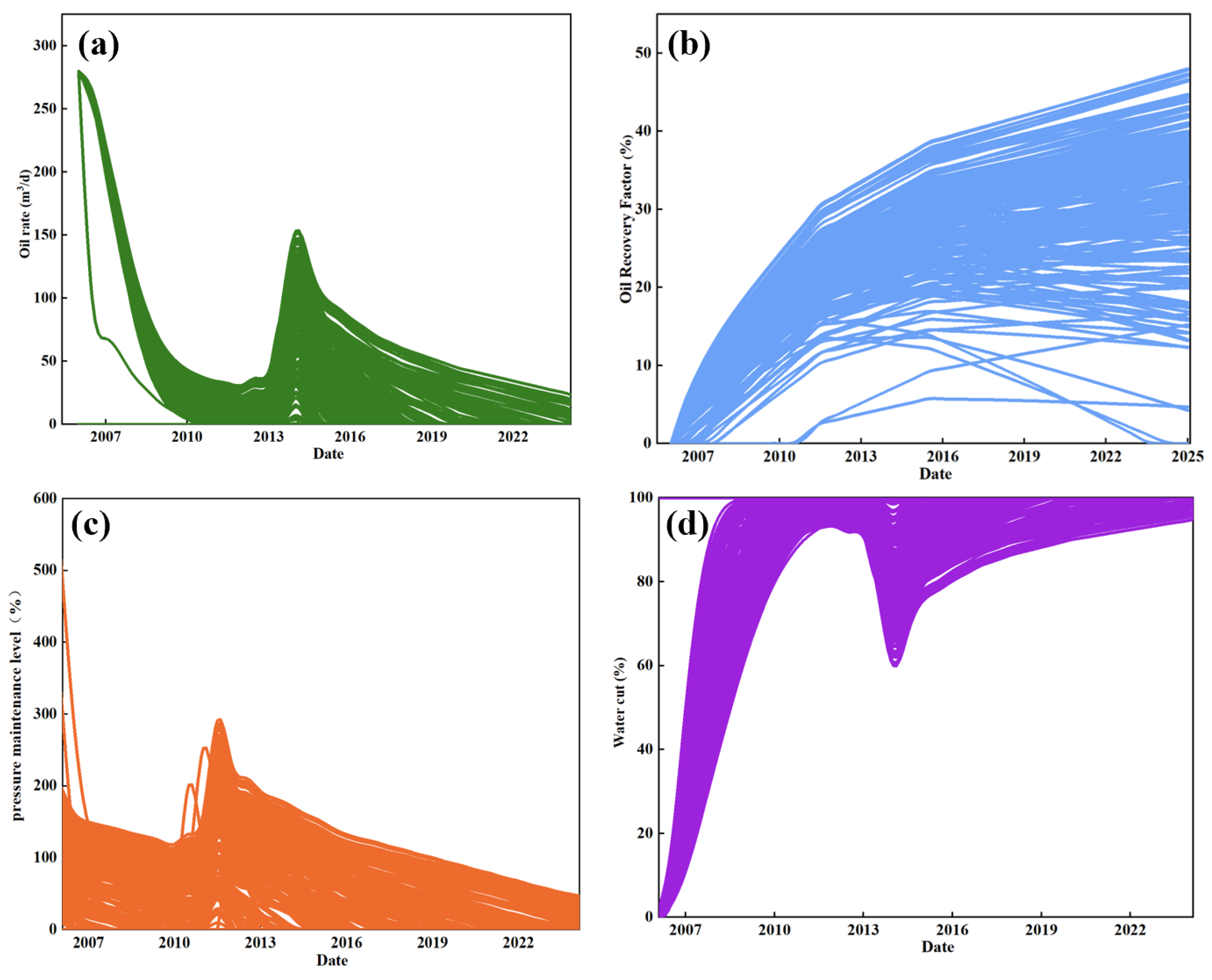
The 800 sets of production curves generated via CMG simulations (Figure 7) comprehensively capture the full-cycle production characteristics, spanning from initial commissioning and production rise to stable production and long-term decline. These profiles provide a rich repository of physical feature samples, enabling the MLR model to effectively learn and characterize the nonlinear fluctuations induced by flow regime transitions under CCCP conditions.

4.2.2. Dataset Construction and Preprocessing Based on LHS and CMG

To eliminate interference from disparate engineering dimensions and ensure efficient gradient descent during training, the raw dataset underwent a specialized preprocessing workflow. Based on the core controlling factors identified in Section 4.1, a “correlation-guided a priori” strategy was implemented: Weighted Feature Enhancement: The comprehensive weight vector W, derived from the fusion of Spearman correlation and EWM, was applied to the standardized original input feature matrix X via a Hadamard Product operation. This ensures that the model focus is physically aligned with the dominant drivers of CCCP dynamics (e.g., production rate and maximum adsorption capacity). Dynamic Scaling: Following the feature weighting, a Min-Max normalization was applied to scale the weighted features into the [0, 1] interval.

4.3. Training and Prediction Performance of the MLR

Taking the weighted and standardized LHS sample set as the input source, a MLR model is constructed to conduct joint training on four core indicators: oil production, water cut, recovery factor and formation pressure maintenance level. The 800 groups of standardized sample data sets are randomly divided into a training set and a validation set at a ratio of 80%:20%, which are input into the MLR model constructed in Section 2.2 for supervised machine learning training. Benefiting from the feature weighting strategy in the early stage, the loss function of the network drops extremely rapidly in the initial stage of training, which not only greatly reduces the number of iteration rounds, but also fundamentally suppresses the overfitting of the model to secondary features with low correlation. With the increase in training iteration times, the loss functions of the MLR model on the training set and validation set both gradually decrease and converge to stable values, while the R² continuously increases and approaches 0.95. This indicates that the model has fully learned the complex production dynamic laws under the chemical composite cold production conditions in the Z well block, and has excellent fitting and generalization abilities for the relationship between core physical parameters and daily oil production. The test results show that the weighted MLR model exhibits excellent fitting accuracy in the prediction of various production indicators, which proves the outstanding effectiveness of the “correlation a priori weight” in driving the nonlinear prediction of complex reservoirs. The test results show that the weighted MLR exhibits excellent fitting accuracy in the prediction of all production indicators such as oil production, water cut, recovery factor and formation pressure maintenance level, and the predicted production dynamic curves are highly consistent with the actual sample curves. This fully proves the outstanding effectiveness of the correlation a priori weight in driving the nonlinear production performance prediction of complex reservoirs, and also verifies the rationality of the pre-stage feature weighting, sample construction and data preprocessing processes.

4.4. Reliability Verification and Efficiency Analysis of the Prediction Model

To rigorously verify the generalization capability of the MLR model, two independent 100-day production sequences (denoted as Sample 1 and Sample 2) were randomly selected from the validation dataset. Notably, these samples represent discontinuous and fragmented time intervals within the reservoir development cycle, which serves as a data shuffling for the model’s ability to capture nonlinear dynamics without relying on temporal continuity.

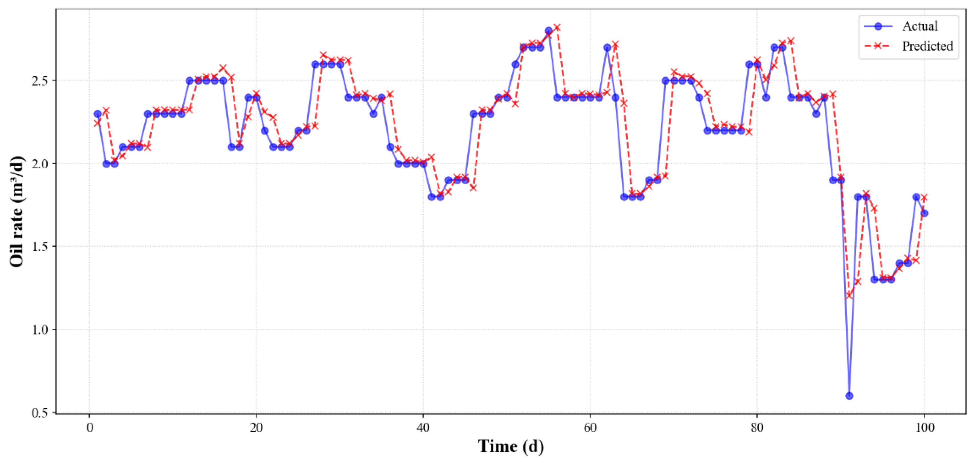
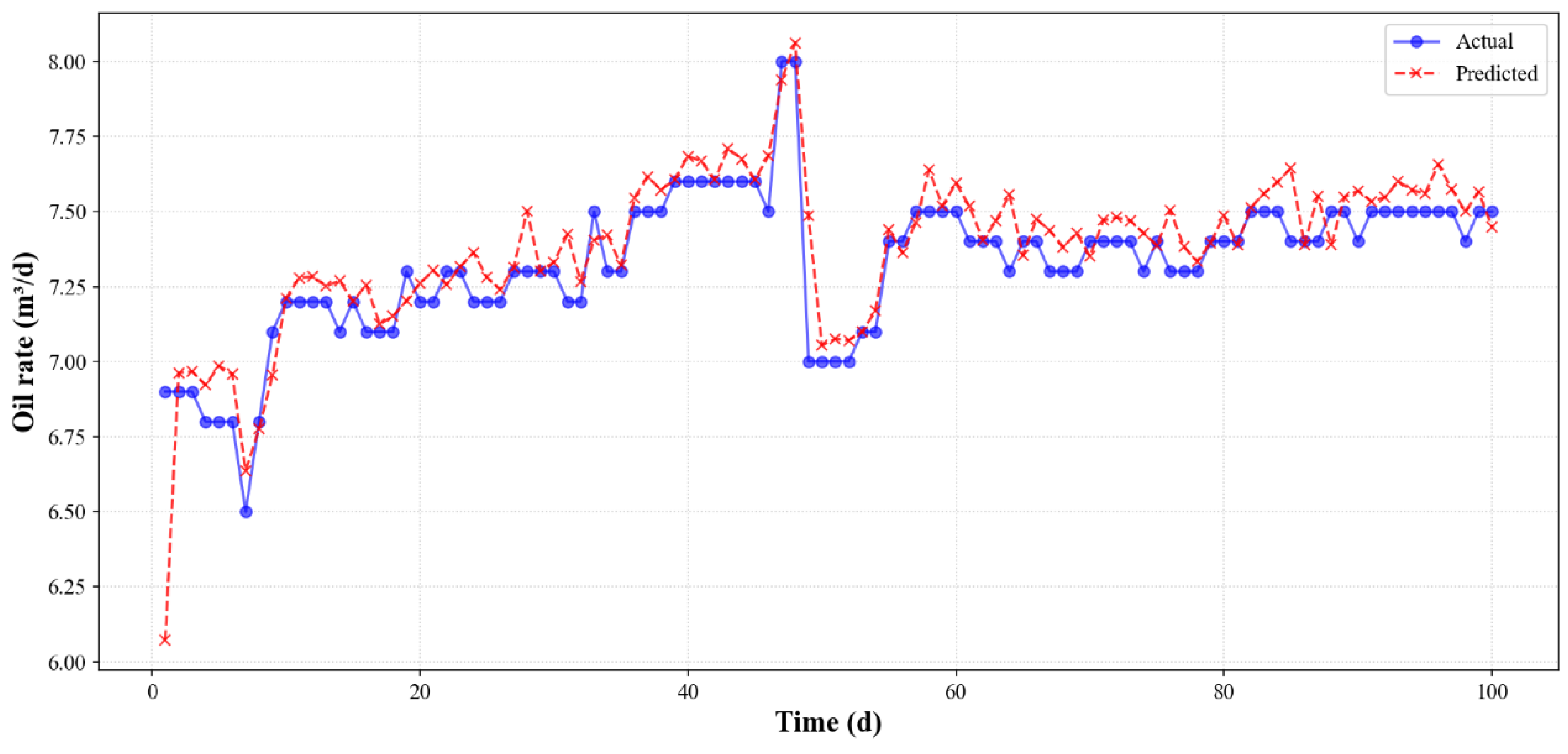
As illustrated in Figure 8 and Figure 9, the predicted oil rate dynamic curves show exceptional overlap with the actual simulation results. This high consistency confirms that the surrogate model has successfully mastered the underlying physical production laws of CCCP rather than simply performing trend extrapolation.

The predictive accuracy was further quantified using three indicators: Mean Absolute Error, Relative Fitting Error, and the Coefficient of Determination R². As detailed in

Table 4. Prediction Performance Metrics on Discontinuous Verification Samples.

Evaluation Metrics	Sample 1	Sample 2
Mean Absolute Error	0.0907	0.0686
Relative Fitting Error	4.01%	1.88%
Coefficient of Determination	0.9538	0.9431

, the relative fitting errors for Sample 1 and Sample 2 are 4.01% and 1.88%, respectively, with R² values reaching 0.9538 and 0.9431. These metrics, particularly the R² values exceeding 0.94, confirm the excellent goodness-of-fit and high reliability of the model. From an engineering perspective, this framework not only ensures high fidelity but also realizes a two-order-of-magnitude increase in computational speed, meeting the requirements for rapid production forecasting and real-time decision-making in oilfield development.

The observed one-step-ahead prediction lag is a common phenomenon in time-series forecasting of dynamic systems, potentially due to the model capturing the underlying physical inertia or transient response rather than instantaneous jumps. This does not significantly impact the medium to long-term trend prediction accuracy crucial for development planning.

5. Conclusions

This study proposes a high-precision, data-driven prediction framework integrating Spearman rank correlation, EWM, and an MLR model to address the nonlinearity challenges in CCCP forecasting. The key conclusions are as follows:

(1) Integrated Feature Weighting and Preprocessing: The dual-driven feature weighting strategy effectively quantifies nonlinear correlations and objective data informativeness. It identifies injection-production balance and development and maximum adsorption capacity as the core controlling factors. This strategy, coupled with correlation-guided weighted standardization, enhances the information density of the feature matrix and eliminates dimensional interference, providing a robust foundation for model training.

(2) Model Performance and Generalization: Utilizing a representative sample space of 800 sets constructed via LHS and CMG simulations (within a ±30% benchmark parameter range), the trained MLR model exhibits exceptional performance. The determination coefficient R² for core indicators exceeds 0.94. Rigorous validation using discontinuous, fragmented production samples (Samples 1 and 2) yielded R² values of 0.9538 and 0.9431, with relative fitting errors below 5%, demonstrating superior generalization capability beyond simple trend extrapolation.

(3) Engineering Efficiency and Practicality: Compared with traditional CMG numerical simulation, the proposed framework reduces single prediction time by over two orders of magnitude while maintaining high precision. By bypassing the over-reliance on intensive history matching and fine geological parameters, this framework enables rapid, real-time, and intelligent production forecasting, providing a high-speed algorithmic solution for the development optimization of heavy oil reservoirs under CCCP.

(4) Future work may incorporate the SHAP (SHapley Additive exPlanations) method to further enhance the interpretability of the machine learning model. By decomposing prediction results at the individual sample level, SHAP can quantify the contribution of each input feature to the final output, reveal the nonlinear response mechanism between key parameters and production performance, and provide more comprehensive, transparent, and physically consistent insights into feature importance and decision logic.

(5) Although the proposed proxy model demonstrates high prediction accuracy and efficiency, several limitations should be acknowledged. First, the model is trained based on numerical simulation data from a specific reservoir (Well Block Z), which may limit its generalization capability when applied to reservoirs with significantly different geological conditions or fluid properties. Second, the current framework assumes relatively stable operational conditions and may not fully capture abrupt changes caused by operational disturbances or extreme production scenarios. Future work will focus on incorporating more diverse field datasets, enhancing model adaptability, and exploring hybrid nonlinear architectures to further improve prediction robustness under complex reservoir conditions.

References

1. Sheikhoushaghi, A.; Gharaei, N.Y.; Nikoofard, A. Application of Rough Neural Network to forecast oil production rate of an oil field in a comparative study. J. Petrol. Sci. Eng. 2022, 209, 109935. [Google Scholar] [CrossRef]
2. Liang, B.; Liu, J.; You, J.; Jia, J.; Pan, Y.; Jeong, H. Hydrocarbon production dynamics forecasting using machine learning: A state-of-the-art review. Fuel 2023, 337, 127067. [Google Scholar] [CrossRef]
3. Rahmanifard, H.; Gates, I. Application of Data Analytic Techniques and Monte-Carlo Simulation for Forecasting and Optimizing Oil Production from Tight Reservoirs. Nat. Resour. Res. 2024, 33, 1685–1701. [Google Scholar] [CrossRef]
4. Rahmanifard, H.; Gates, I. A Comprehensive review of data-driven approaches for forecasting production from unconventional reservoirs: Best practices and future directions. Artif. Intell. Rev. 2024, 57, 213. [Google Scholar] [CrossRef]
5. Zhao, Y.; Luo, R.; Li, L.; Zhang, R.; Zhang, D.; Zhang, T.; Xie, Z.; Luo, S.; Zhang, L. A review on optimization algorithms and surrogate models for reservoir automatic history matching. Geoenergy Sci. Eng. 2024, 233, 212554. [Google Scholar] [CrossRef]
6. Samnioti, A.; Gaganis, V. Applications of Machine Learning in Subsurface Reservoir Simulation—A Review—Part I. Energies 2023, 16, 6079. [Google Scholar] [CrossRef]
7. Cirac, G.; Farfan, J.; Avansi, G.D.; Schiozer, D.J.; Rocha, A. Cross-Domain Feature learning and data augmentation for few-shot proxy development in oil industry. Appl. Soft Comput. 2023, 149, 110972. [Google Scholar] [CrossRef]
8. Pan, S.; Yang, B.; Wang, S.; Guo, Z.; Wang, L.; Liu, J.; Wu, S. Oil well production prediction based on CNN-LSTM model with self-attention mechanism. Energy 2023, 284, 128701. [Google Scholar] [CrossRef]
9. Hu, C.; Zhong, Y.; Lu, Y.; Luo, X.; Wang, S. A Prediction Model for Time Series of Dissolved Gas Content in Transformer Oil Based on LSTM. J. Phys. Conf. Ser. 2020, 1659, 012030. [Google Scholar] [CrossRef]
10. Zhou, G.; Guo, Z.; Sun, S.; Jin, Q. A CNN-BiGRU-AM neural network for AI applications in shale oil production prediction. Appl. Energy 2023, 344, 121249. [Google Scholar] [CrossRef]
11. Zha, W.; Liu, Y.; Wan, Y.; Luo, R.; Li, D.; Yang, S.; Xu, Y. Forecasting monthly gas field production based on the CNN-LSTM model. Energy 2022, 260, 124889. [Google Scholar] [CrossRef]
12. Qiu, B.; Zhang, J.; Yang, Y.; Qin, G.; Zhou, Z.; Ying, C. Research on Oil Well Production Prediction Based on GRU-KAN Model Optimized by PSO. Energies 2024, 17, 5502. [Google Scholar] [CrossRef]
13. Chen, G.; Tian, H.; Xiao, T.; Xu, T.; Lei, H. Time series forecasting of oil production in Enhanced Oil Recovery system based on a novel CNN-GRU neural network. Geoenergy Sci. Eng. 2024, 233, 212528. [Google Scholar] [CrossRef]
14. Kocoglu, Y.; Gorell, S.B.; Emadi, H.; Eyinla, D.S.; Bolouri, F.; Kocoglu, Y.C.; Arora, A. Improving the accuracy of short-term multiphase production forecasts in unconventional tight oil reservoirs using contextual Bi-directional long short-term memory. Geoenergy Sci. Eng. 2024, 235, 212688. [Google Scholar] [CrossRef]
15. You, H.; Yu, Y.; Silling, S.; D’Elia, M. A data-driven peridynamic continuum model for upscaling molecular dynamics. Comput. Method Appl. M 2022, 389, 114400. [Google Scholar] [CrossRef]
16. Yan, B.; Zhong, Z.; Bai, B. A convolutional neural network-based proxy model for field production prediction and history matching. Gas Sci. Eng. 2024, 122, 205219. [Google Scholar] [CrossRef]
17. Karniadakis, G.E.; Kevrekidis, I.G.; Lu, L.; Perdikaris, P.; Wang, S.; Yang, L. Physics-informed machine learning. Nat. Rev. Phys. 2021, 3, 422–440. [Google Scholar] [CrossRef]
18. Cuomo, S.; Di Cola, V.S.; Giampaolo, F.; Rozza, G.; Raissi, M.; Piccialli, F. Scientific machine learning through physics-informed neural networks: Where we are and what’s next. J. Sci. Comput. 2022, 92, 88. [Google Scholar] [CrossRef]
19. Wang, N.; Zhang, H.; Chang, H.; Zhang, Y.; Feng, Q.; Zhang, J. A physics-informed neural network-enhanced capacitance resistance model for production forecasting in offshore fields. Geoenergy Sci. Eng. 2024, 238, 212885. [Google Scholar] [CrossRef]
20. Zhong, Z.; Sun, A.Y.; Yang, Q.; Ouyang, Q. A deep learning-physics hybrid framework for accurate and interpretable subsurface flow prediction. J. Hydrol. 2023, 625, 130090. [Google Scholar] [CrossRef]
21. Wang, S.; Qin, C.; Feng, Q.; Javadpour, F.; Rui, Z. A hybrid physics-machine learning model for forecasting oil production in unconventional reservoirs. SPE J. 2024, 29, 2450–2467. [Google Scholar] [CrossRef]
22. Zhou, L.; Zhang, R.-H. A hybrid neural network model for ENSO prediction in combination with principal oscillation pattern analyses. Adv. Atmos. Sci. 2022, 39, 889–902. [Google Scholar] [CrossRef]
23. Liu, W.; Liu, W.D.; Gu, J. Forecasting oil production using ensemble learning integrating extreme gradient boosting and the water drive characteristic curve. Pet Sci. 2024, 21, 1890–1903. [Google Scholar] [CrossRef]
24. Lundberg, S.M.; Lee, S.I. A unified approach to interpreting model predictions. Adv. Neural Inf. Process. Syst. 2017, 30, 4765–4774. [Google Scholar]
25. Samek, W.; Montavon, G.; Vedaldi, A.; Hansen, L.K.; Müller, K.R. Explainable AI: Interpreting, Explaining and Visualizing Deep Learning; Springer: Cham, Switzerland, 2019. [Google Scholar] [CrossRef]
26. Goswami, S.; Yin, M.; Yu, Y.; Karniadakis, G.E. A physics-informed variational DeepONet for predicting crack propagation in brittle materials. Comput. Method Appl. M 2022, 391, 114587. [Google Scholar] [CrossRef]
27. Song, F.; Ding, H.; Wang, Y.; Zhang, S.; Yu, J. A Well Production Prediction Method of Tight Reservoirs Based on a Hybrid Neural Network. Energies 2023, 16, 2904. [Google Scholar] [CrossRef]
28. Maldonado-Cruz, E.; Pyrcz, M.J. Multi-horizon well performance forecasting with temporal fusion transformers. Results Eng. 2024, 21, 101776. [Google Scholar] [CrossRef]
29. Ye, F.; Li, X.; Zhang, N.; Xu, F. Prediction of Single-Well Production Rate after Hydraulic Fracturing in Unconventional Gas Reservoirs Based on Ensemble Learning Model. Processes 2024, 12, 1194. [Google Scholar] [CrossRef]
30. Gu, D.; Zheng, R.; Cheng, P.; Zhou, S.; Yan, G.; Liu, H.; Yang, K.; Wang, J.; Zhu, Y.; Liao, M. Single Well Production Prediction Model of Gas Reservoir Based on CNN-BILSTM-AM. Energies 2024, 17, 5674. [Google Scholar] [CrossRef]
31. Zhao, G.; Ding, W.; Tian, J.; Liu, J.; Gu, Y.; Shi, S.; Wang, R.; Sun, N. Spearman rank correlations analysis of the elemental, mineral concentrations, and mechanical parameters of the Lower Cambrian Niutitang shale: A case study in the Fenggang block, Northeast Guizhou Province, South China. J. Petrol. Sci. Eng. 2022, 208, 109550. [Google Scholar] [CrossRef]
32. Zheng, H.; Yang, Z.; Yang, J.; Tao, Y.; Zhang, L. Comprehensive Evaluation of Environmental Air Quality Based on the Entropy Weights and Concentration Variation Trends of Pollutants. Atmosphere 2022, 13, 1978. [Google Scholar] [CrossRef]
33. von Hohendorff Filho, J.C.; Maschio, C.; Schiozer, D.J. Production strategy optimization based on iterative discrete Latin hypercube. J. Braz. Soc. Mech. Sci. 2016, 38, 2473–2480. [Google Scholar] [CrossRef]
34. Pripp, A.H. Pearson’s or Spearman’s correlation coefficients. Tidsskr. Den Nor. Laegeforening Tidsskr. Prakt. Med. Ny Raekke 2018, 138, 10–4045. [Google Scholar] [CrossRef]
35. Dang, C.; Nghiem, L.; Nguyen, N.; Yang, C.; Chen, Z.; Bae, W. Modeling and optimization of alkaline-surfactant-polymer flooding and hybrid enhanced oil recovery processes. J. Petrol. Sci. Eng. 2018, 169, 578–601. [Google Scholar] [CrossRef]
Figure 1. Schematic of the proposed Feature Importance Analysis methodology. (a) EWM weighting mechanism, and (b) RF ensemble learning structure.
Processes 14 01050 g001
Figure 2. Numerical simulation model characterization, (a) permeability, (b) porosity, and (c) oil saturation.
Processes 14 01050 g002
Figure 3. Production Performance Curves. (a) Oil rate, (b) water cut, (c) oil recovery factor, and (d) pressure maintenance level.
Processes 14 01050 g003
Figure 4. History Matching. (a) Oil rate, (b) oil recovery factor, (c) water cut, and (d) pressure maintenance level.
Processes 14 01050 g004
Figure 5. Spearman correlation heatmaps. (a) feature-to-feature correlation, and (b) feature-to-target correlation.
Processes 14 01050 g005
Figure 6. Distribution of Indicator Weights.
Processes 14 01050 g006
Figure 7. Representative training datasets generated via LHS and CMG simulations. (a) Oil rate, (b) oil recovery factor, (c) pressure maintenance level, and (d) water cut.
Processes 14 01050 g007
Figure 8. Dynamic fitting of oil production rate for Validation Sample 1.
Processes 14 01050 g008
Figure 9. Comparison between actual and predicted oil rate dynamics for Validation Sample 2.
Processes 14 01050 g009