Channel Wave Advanced Detection by Reverse-Time Migration Based on the Curvilinear Grid Finite-Difference Method

Abstract

Accurate identification of concealed coal seam structures, such as folds or faults, is crucial for safe and effective production in the coal mining industry. In-seam seismic exploration serves as a promising technique for advanced detection of coal seam structures, but traditional numerical simulation methods easily produce errors when coping with irregular interfaces. This study uses the curvilinear grid finite-difference method (FDM) for modeling the 3D channel wave propagation. The body-fitted grids are utilized to conform to undulating interfaces, while the DRP/opt MacCormack difference scheme and the fourth-order Runge–Kutta algorithm are applied for the spatial and temporal derivative approximation, in that order. The forward and backward extrapolation for in-seam waves are implemented in the curvilinear coordinates. The roofs and floors of coal seams and special structures are imaged by reverse-time migration (RTM) using an excitation amplitude imaging condition. Numerical results show that compared with conventional methods, the curvilinear grid method effectively reduces spurious scattering caused by the staircase approximation, improves the modeling accuracy of channel waves, and enhances the continuity and interpretability of imaged coal-seam interfaces and structural boundaries. The proposed method has the potential to enhance the accuracy of channel wave exploration under complex geological conditions, supporting advanced hazard detection in coal mines.

1. Introduction

Higher demands have arisen for the precise characterization of underground geological structures and the accurate prediction of coal seam occurrence conditions as a result of the coal industry’s deep transformation toward “less manpower, unmanned” and the advancement of intelligent coal mine construction [1,2,3]. In this context, leveraging advanced geophysical exploration technologies to achieve detailed characterization of complex coal seam occurrence conditions has become a critical factor in ensuring safe, efficient, and intelligent mining of coal mines [4]. As one of the most effective methods for underground coal mine detection, channel-wave seismic exploration utilizes guided waves generated and propagated within coal seams to detect coal seam discontinuities by analyzing their propagation characteristics [5]. This technique has proven effective in characterizing internal coal seam structure development, coal seam thickness fluctuations, paleochannel scours, and gangue distribution patterns [6], becoming a critical technical pillar for probing macroscopic geological structures as well as concealed hazard-inducing features (e.g., faults, collapsed columns). Notably, reflected channel wave detection can be conducted in single tunnels during excavation, featuring low construction condition requirements, and is capable of detecting geological structures along roadway walls and ahead, serving as a vital method for identifying geological anomalies in underground coal mines [7,8]. Studying the propagation behaviors of reflected channel waves within coal-rock masses using numerical simulation can offer theoretical guidance for data acquisition, processing, and interpretation in mine seismic advance detection.

Currently, the numerical simulation methods for channel waves mainly consist of the finite-difference method (FDM) [9], the finite element method (FEM) [10], and the analytical approach [11]. Early studies mostly focused on numerical simulation and dispersion analysis. Krey calculated the dispersion profiles for Love waves and Rayleigh waves within horizontally layered coal seams, confirming the existence of in-seam waves within coal seams [12]. Asten et al. investigate the dispersion properties of Love-type in-seam waves within coal seam models containing faults using the FEM [13]. Lou et al. simulated Love-type in-seam waves within two-dimensional thin-layered anisotropic media, verifying the significant influence of anisotropy on dispersion [14]. Ji et al. first achieved 3D channel wave numerical simulation for coal seam models with roadways by virtue of the principles underlying the FDM and mirror image method [15]. Qiao et al. simulated Rayleigh-type channel waves using the spectral element method and systematically analyzed the dispersion properties of Rayleigh-type in-seam wavefields within coal seam models containing small faults [16]. The spectral element method exhibits high simulation accuracy under complex geometric conditions, but its mesh generation and computational resource requirements are generally higher. In contrast, the FDM remains more commonly used in engineering applications for 3D channel wave simulations due to its advantages of simplicity in implementation and high efficiency. In recent years, relevant studies have been further broadened to include anisotropic and viscoelastic geological media. Ji et al. [17] and Jiao et al. [18] respectively adopted the staggered grid high-order FDM for the investigation of 3D channel wavefields in HTI coal seam media and viscoelastic VTI coal seam media. Wu implemented 3D channel wave simulations for fault and fold models employing the staggered grid high-order FDM, comparing the waveform characteristics and dispersion properties between the two models [19]. However, when describing undulating coal seam interfaces, current approaches still face the problem of false scattering resulting from staircase approximation.

The FDM is the predominant technique for seismic wave simulation due to its high computational efficiency and straightforward programming implementation. However, conventional Cartesian-coordinate-based FDM with rectangular or cuboid grids usually adopts stair-case grid approximation when fitting undulating ground surfaces or irregular medium interfaces, which generates artificial scattering and thus degrades simulation accuracy [20]. Various grid improvement strategies have been developed to enhance the capability of the FDM in characterizing complex interfaces. For instance, the unstructured grid FDM can more precisely fit curved interfaces and achieve local mesh refinement through triangular/tetrahedral discretization, but its mesh generation and differential operator construction are generally cumbersome with high computational costs. The variable grid FDM reduces the staircase approximation error by densifying the sampling near undulating interfaces, yet it may still retain spurious scattering at the interface [21]. In contrast, the curvilinear grid FDM precisely conforms to the undulating interfaces while maintaining computational efficiency, thereby effectively suppressing the scattering artifacts caused by staircase approximations. Zhang et al. were among the first to incorporate body-fitted grids into this method. They realized the forward simulation of seismic waves for isotropic and anisotropic geological media under undulating ground surfaces based on collocated grids and further developed the traction mirror method in curvilinear grids to effectively handle free-surface boundary conditions [22,23,24,25]. Nevertheless, channel wave numerical simulation has seldom addressed the effects of roof-floor interface undulations within the coal seam on channel-wave propagation. Therefore, applying the curvilinear grid FDM to channel wave modeling plays a vital role in enhancing simulation accuracy under complex geological conditions.

Building on high-accuracy numerical modeling results, channel wave imaging enables the characterization of subsurface structures’ spatial distribution (e.g., folds, faults, and collapse columns), which is a key step for accurately identifying coal seam geological structures. At present, reflected channel wave imaging methods are mainly divided into two categories: stacking-based imaging and migration-based imaging. The stacking imaging method for reflected channel waves is analogous to the stacking method used in surface 2D seismic surveys; however, as the angle between the fault azimuth and the survey line increases, the effectiveness of the stacking method decreases accordingly, making it difficult to correctly image the target interfaces. Among migration-based methods, diffraction migration imaging based on ray theory has been most widely applied. Recently, Wang et al. [8] and Wu [19] have applied this method to the detection of goaf roadways and the identification of faults and folds, respectively. In contrast, research on the application of wave equation-based reverse-time migration (RTM) in channel wave imaging remains quite limited. Currently, only Hu et al. have attempted to introduce RTM technology into reflected channel wave imaging and tested it using model data [26]. Given that RTM performs full-wavefield reverse-time extrapolation by virtue of the two-way wave equation, it exhibits notable superiority over Kirchhoff migration and one-way wave migration in imaging accuracy, amplitude preservation, and adaptability to structures with arbitrary dip angles [27,28]. Therefore, investigating RTM imaging for channel waves plays a significant role in promoting channel wave imaging quality and detection reliability.

Compared with previous studies, which predominantly rely on Cartesian grid FDM and stacking- or ray-based channel wave imaging, the present work introduces a curvilinear grid FDM framework that more accurately conforms to strongly undulating roof–floor interfaces. Additionally, this approach is coupled with wave equation-based RTM for reflected channel wave imaging. This combination effectively mitigates staircase approximation-induced scattering artifacts in numerical modeling and improves the imaging quality of subsurface geological discontinuities, particularly in complex geological geometries.

With the extension of coal mining toward deeper and more complex areas, higher requirements have been imposed on the precision and resolution of channel wave exploration, particularly in identifying small-scale structures such as faults with throws of less than 5 m, minor folds, and small collapse columns. To address these demands, this paper adopts the FDM based on curvilinear grids presented by Zhang and Chen [22] for 3D channel wave numerical simulation and RTM imaging in complex coal seams. First, the first-order velocity-stress elastic wave equation in the curvilinear coordinate system is derived. The DRP/opt MacCormack difference scheme and the fourth-order Runge–Kutta method are then employed to discretize the spatial and temporal partial derivatives in the wave equation, thereby realizing 3D channel wave forward modeling for curved coal seam models containing either folds or faults using the curvilinear grid FDM. Building on these simulations, the excitation amplitude imaging condition is adopted to implement channel wave RTM imaging. Through systematic comparison with Cartesian grid simulations and imaging results, the effectiveness of curvilinear grids in improving simulation precision and imaging accuracy is validated. The present work is intended to establish the theoretical foundation and provide methodological support for high-resolution detection of underground geological anomalies in coal mines.

2. Methods

2.1. Reflected Channel Wave Detection Technique

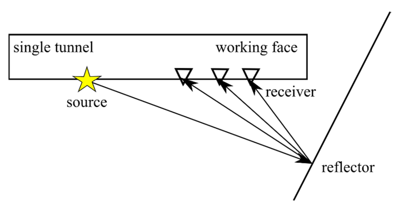
Compared with surrounding rocks, coal seams have low wave velocity and low density. This difference in wave impedance enables coal seams to act as natural seismic waveguides. Once a seismic source is activated inside the coal seam, body waves undergo multiple total reflections at the roof and floor interfaces of coal seams, becoming confined to propagate within the coal seam and its adjacent rocks (referred to as the coal channel), without radiating energy into the surrounding rocks. These confined body waves superimpose and interfere with the coal channel, forming guided waves that propagate along the coal seam, known as channel waves [29]. Reflected channel waves are generated at reflection interfaces with significant impedance contrasts when they encounter changes in the propagation medium (e.g., faults, folds, and other abnormal geological structures) during their propagation in coal seams. As illustrated in Figure 1, the reflected channel wave method relies on deploying a seismic source and a geophone array within the same coal roadway to excite and record reflected channel-wave signals. Reflecting interfaces are then identified from the seismic records, allowing for the inference of the locations of faults and other geological anomalies in the coal seam.

2.2. Curvilinear Grid Finite Difference Algorithm

2.2.1. First-Order Velocity-Stress Equations in Curvilinear Coordinate System

The form of the 3D first-order velocity-stress elastic wave equations is given by:

$$\left\{\begin{array}{l}\rho {\displaystyle \frac{\partial V_x}{\partial t}}={\displaystyle \frac{\partial {\sigma }_{xx}}{\partial x}}+{\displaystyle \frac{\partial {\sigma }_{xy}}{\partial y}}+{\displaystyle \frac{\partial {\sigma }_{xz}}{\partial z}}\\ \rho {\displaystyle \frac{\partial V_y}{\partial t}}={\displaystyle \frac{\partial {\sigma }_{xy}}{\partial x}}+{\displaystyle \frac{\partial {\sigma }_{yy}}{\partial y}}+{\displaystyle \frac{\partial {\sigma }_{yz}}{\partial z}}\\ \rho {\displaystyle \frac{\partial V_z}{\partial t}}={\displaystyle \frac{\partial {\sigma }_{xz}}{\partial x}}+{\displaystyle \frac{\partial {\sigma }_{yz}}{\partial y}}+{\displaystyle \frac{\partial {\sigma }_{zz}}{\partial z}}\\ {\displaystyle \frac{\partial {\sigma }_{xx}}{\partial t}}=\left(\lambda +2\mu \right){\displaystyle \frac{\partial V_x}{\partial x}}+\lambda \left({\displaystyle \frac{\partial V_z}{\partial z}}+{\displaystyle \frac{\partial V_y}{\partial y}}\right)\\ {\displaystyle \frac{\partial {\sigma }_{yy}}{\partial t}}=\left(\lambda +2\mu \right){\displaystyle \frac{\partial V_y}{\partial y}}+\lambda \left({\displaystyle \frac{\partial V_x}{\partial x}}+{\displaystyle \frac{\partial V_z}{\partial z}}\right)\\ {\displaystyle \frac{\partial {\sigma }_{zz}}{\partial t}}=\left(\lambda +2\mu \right){\displaystyle \frac{\partial V_z}{\partial z}}+\lambda \left({\displaystyle \frac{\partial V_x}{\partial x}}+{\displaystyle \frac{\partial V_y}{\partial y}}\right)\\ {\displaystyle \frac{\partial {\sigma }_{yz}}{\partial t}}=\mu \left({\displaystyle \frac{\partial V_z}{\partial y}}+{\displaystyle \frac{\partial V_y}{\partial z}}\right)\\ {\displaystyle \frac{\partial {\sigma }_{xz}}{\partial t}}=\mu \left({\displaystyle \frac{\partial V_z}{\partial x}}+{\displaystyle \frac{\partial V_x}{\partial z}}\right)\\ {\displaystyle \frac{\partial {\sigma }_{xy}}{\partial t}}=\mu \left({\displaystyle \frac{\partial V_x}{\partial y}}+{\displaystyle \frac{\partial V_y}{\partial x}}\right)\end{array}\right.$$

(1)

where ρ is the medium density, $\left[V_x,V_y,V_z\right]$ denotes the particle polarization velocity, and t is time. $\left[{\sigma }_{xx},{\sigma }_{yy},{\sigma }_{zz}\right]$ and $\left[{\sigma }_{yz},{\sigma }_{xz},{\sigma }_{xy}\right]$ represent the normal- and shear-stress components, respectively. The Lamé constants are λ and μ, with $\lambda =\rho \left(V_{\mathrm{P}}^2-2V_{\mathrm{S}}^2\right)$ and $\mu =\rho V_{\mathrm{S}}^2$. $V_P$ and $V_S$ denote the P-wave and S-wave velocities of the medium, in that order.

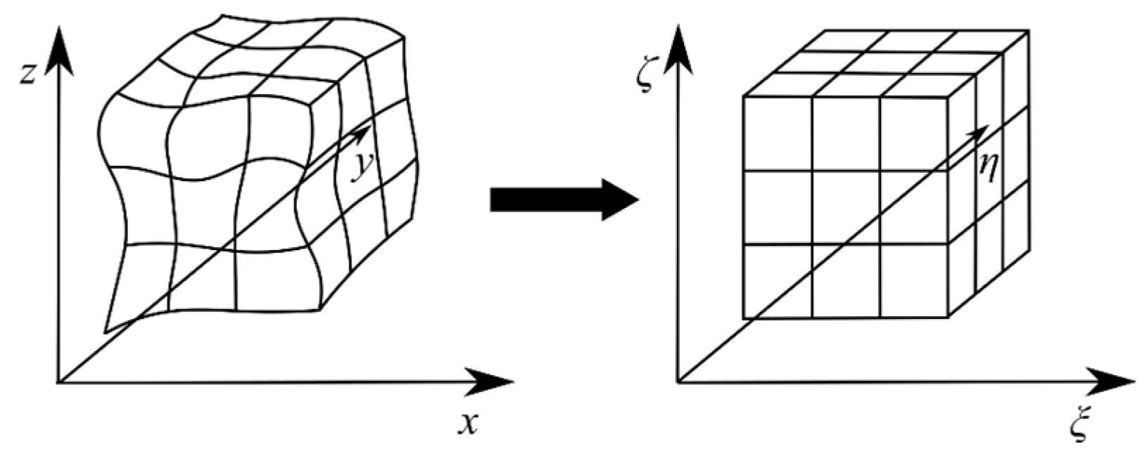
Within the curvilinear coordinate system, curvilinear grid generation essentially lies in coordinate transformation, i.e., mapping the irregular domain in the physical region to the regular domain in the computational region. Figure 2 illustrates a schematic of the coordinate transformation relationship between 3D curvilinear grids and Cartesian grids. The computational region grid coordinates $\left(\xi ,\eta ,\zeta \right)$ satisfy the following relation with the physical domain grid coordinates $\left(x,y,z\right)$:

$$\left\{\begin{array}{l}x=x\left(\xi ,\eta ,\zeta \right)\\ y=y\left(\xi ,\eta ,\zeta \right)\\ z=z\left(\xi ,\eta ,\zeta \right)\end{array}\right.$$

(2)

Based on the above mapping relationship, the following identity can be derived:

$$\left(\begin{array}{ccc}{x}_{,\xi }& x_{,\eta }& x_{,\zeta }\\ y_{,\xi }& y_{,\eta }& y_{,\zeta }\\ z_{,\xi }& z_{,\eta }& z_{,\zeta }\end{array}\right)\left(\begin{array}{ccc}{\xi }_{,x}& {\xi }_{,y}& {\xi }_{,z}\\ {\eta }_{,x}& {\eta }_{,y}& {\eta }_{,z}\\ {\zeta }_{,x}& {\zeta }_{,y}& {\zeta }_{,z}\end{array}\right)=\left(\begin{array}{ccc}1& 0& 0\\ 0& 1& 0\\ 0& 0& 1\end{array}\right)$$

(3)

where $m_{,n}$ denotes the derivative operation of coordinate m with respect to coordinate n.

The inverse coordinate transformation coefficients are obtained by solving Equation (3):

$$\begin{array}{l}{\xi }_{,x}={\displaystyle \frac{1}{J}}\left(y_{,\eta }{z}_{,\zeta }-y_{,\zeta }{z}_{,\eta }\right)\hspace{1em}\hspace{1em}{\xi }_{,y}={\displaystyle \frac{1}{J}}\left(x_{,\zeta }{z}_{,\eta }-x_{,\eta }{z}_{,\zeta }\right)\hspace{1em}\hspace{1em}{\xi }_{,z}={\displaystyle \frac{1}{J}}\left(x_{,\eta }{y}_{,\zeta }-x_{,\zeta }{y}_{,\eta }\right)\\ {\eta }_{,x}={\displaystyle \frac{1}{J}}\left(y_{,\zeta }{z}_{,\xi }-y_{,\xi }{z}_{,\zeta }\right)\hspace{1em}\hspace{1em}{\eta }_{,y}={\displaystyle \frac{1}{J}}\left(x_{,\xi }{z}_{,\zeta }-x_{,\zeta }{z}_{,\xi }\right)\hspace{1em}\hspace{1em}{\eta }_{,z}={\displaystyle \frac{1}{J}}\left(x_{,\zeta }{y}_{,\xi }-x_{,\xi }{y}_{,\zeta }\right)\\ {\zeta }_{,x}={\displaystyle \frac{1}{J}}\left(y_{,\xi }{z}_{,\eta }-y_{,\eta }{z}_{,\xi }\right)\hspace{1em}\hspace{1em}{\zeta }_{,y}={\displaystyle \frac{1}{J}}\left(x_{,\eta }{z}_{,\xi }-x_{,\xi }{z}_{,\eta }\right)\hspace{1em}\hspace{1em}{\zeta }_{,z}={\displaystyle \frac{1}{J}}\left(x_{,\xi }{y}_{,\eta }-x_{,\eta }{y}_{,\xi }\right)\end{array}$$

(4)

where J is the Jacobian determinant. To ensure that the generated grid remains distortion-free, it is essential to guarantee that $J\ne 0$ throughout the computational domain. The Jacobian determinant is expressed as:

$$J=\left|\begin{array}{ccc}{x}_{,\xi }& x_{,\eta }& x_{,\zeta }\\ y_{,\xi }& y_{,\eta }& y_{,\zeta }\\ z_{,\xi }& z_{,\eta }& z_{,\zeta }\end{array}\right|$$

(5)

According to the chain rule, it is feasible to extend the first-order velocity-stress equations from Cartesian grids to curvilinear coordinate systems. The formula corresponding to the first-order velocity-stress equation in the curvilinear coordinate system is:

$$\begin{array}{cc}\rho {\displaystyle \frac{\partial V_x}{\partial t}}& ={\xi }_{,x}{\sigma }_{xx,\xi }+{\xi }_{,y}{\sigma }_{xy,\xi }+{\xi }_{,z}{\sigma }_{xz,\xi }\\ & +{\eta }_{,x}{\sigma }_{xx,\eta }+{\eta }_{,y}{\sigma }_{xy,\eta }+{\eta }_{,z}{\sigma }_{xz,\eta }\\ & +{\zeta }_{,x}{\sigma }_{xx,\zeta }+{\zeta }_{,y}{\sigma }_{xy,\zeta }+{\zeta }_{,z}{\sigma }_{xz,\zeta }\end{array}$$

(6)

$$\begin{array}{cc}\rho {\displaystyle \frac{\partial V_y}{\partial t}}& ={\xi }_{,x}{\sigma }_{xy,\xi }+{\xi }_{,y}{\sigma }_{yy,\xi }+{\xi }_{,z}{\sigma }_{yz,\xi }\\ & +{\eta }_{,x}{\sigma }_{xy,\eta }+{\eta }_{,y}{\sigma }_{yy,\eta }+{\eta }_{,z}{\sigma }_{yz,\eta }\\ & +{\zeta }_{,x}{\sigma }_{xy,\zeta }+{\zeta }_{,y}{\sigma }_{yy,\zeta }+{\zeta }_{,z}{\sigma }_{yz,\zeta }\end{array}$$

(7)

$$\begin{array}{cc}\rho {\displaystyle \frac{\partial V_z}{\partial t}}& ={\xi }_{,x}{\sigma }_{xz,\xi }+{\xi }_{,y}{\sigma }_{yz,\xi }+{\xi }_{,z}{\sigma }_{zz,\xi }\\ & +{\eta }_{,x}{\sigma }_{xz,\eta }+{\eta }_{,y}{\sigma }_{yz,\eta }+{\eta }_{,z}{\sigma }_{zz,\eta }\\ & +{\zeta }_{,x}{\sigma }_{xz,\zeta }+{\zeta }_{,y}{\sigma }_{yz,\zeta }+{\zeta }_{,z}{\sigma }_{zz,\zeta }\end{array}$$

(8)

$$\begin{array}{cc}{\displaystyle \frac{\partial {\sigma }_{xx}}{\partial t}}& =\left(\lambda +2\mu \right){\xi }_{,x}{V}_{x,\xi }+\lambda {\xi }_{,y}{V}_{y,\xi }+\lambda {\xi }_{,z}{V}_{z,\xi }\\ & +\left(\lambda +2\mu \right){\eta }_{,x}{V}_{x,\eta }+\lambda {\eta }_{,y}{V}_{y,\eta }+\lambda {\eta }_{,z}{V}_{z,\eta }\\ & +\left(\lambda +2\mu \right){\zeta }_{,x}{V}_{x,\zeta }+\lambda {\zeta }_{,y}{V}_{y,\zeta }+\lambda {\zeta }_{,z}{V}_{z,\zeta }\end{array}$$

(9)

$$\begin{array}{cc}{\displaystyle \frac{\partial {\sigma }_{yy}}{\partial t}}& =\lambda {\xi }_{,x}{V}_{x,\xi }+\left(\lambda +2\mu \right){\xi }_{,y}{V}_{y,\xi }+\lambda {\xi }_{,z}{V}_{z,\xi }\\ & +\lambda {\eta }_{,x}{V}_{x,\eta }+\left(\lambda +2\mu \right){\eta }_{,y}{V}_{y,\eta }+\lambda {\eta }_{,z}{V}_{z,\eta }\\ & +\lambda {\zeta }_{,x}{V}_{x,\zeta }+\left(\lambda +2\mu \right){\zeta }_{,y}{V}_{y,\zeta }+\lambda {\zeta }_{,z}{V}_{z,\zeta }\end{array}$$

(10)

$$\begin{array}{cc}{\displaystyle \frac{\partial {\sigma }_{zz}}{\partial t}}& =\lambda {\xi }_{,x}{V}_{x,\xi }+\lambda {\xi }_{,y}{V}_{y,\xi }+\left(\lambda +2\mu \right){\xi }_{,z}{V}_{z,\xi }\\ & +\lambda {\eta }_{,x}{V}_{x,\eta }+\lambda {\eta }_{,y}{V}_{y,\eta }+\left(\lambda +2\mu \right){\eta }_{,z}{V}_{z,\eta }\\ & +\lambda {\zeta }_{,x}{V}_{x,\zeta }+\lambda {\zeta }_{,y}{V}_{y,\zeta }+\left(\lambda +2\mu \right){\zeta }_{,z}{V}_{z,\zeta }\end{array}$$

(11)

$$\begin{array}{cc}{\displaystyle \frac{\partial {\sigma }_{xy}}{\partial t}}& =\mu \left({\xi }_{,y}{V}_{x,\xi }+{\xi }_{,x}{V}_{y,\xi }\right)\\ & +\mu \left({\eta }_{,y}{V}_{x,\eta }+{\eta }_{,x}{V}_{y,\eta }\right)\\ & +\mu \left({\zeta }_{,y}{V}_{x,\zeta }+{\zeta }_{,x}{V}_{y,\zeta }\right)\end{array}$$

(12)

$$\begin{array}{cc}{\displaystyle \frac{\partial {\sigma }_{xz}}{\partial t}}& =\mu \left({\xi }_{,z}{V}_{x,\xi }+{\xi }_{,x}{V}_{z,\xi }\right)\\ & +\mu \left({\eta }_{,z}{V}_{x,\eta }+{\eta }_{,x}{V}_{z,\eta }\right)\\ & +\mu \left({\zeta }_{,z}{V}_{x,\zeta }+{\zeta }_{,x}{V}_{z,\zeta }\right)\end{array}$$

(13)

$$\begin{array}{cc}{\displaystyle \frac{\partial {\sigma }_{yz}}{\partial t}}& =\mu \left({\xi }_{,z}{V}_{y,\xi }+{\xi }_{,y}{V}_{z,\xi }\right)\\ & +\mu \left({\eta }_{,z}{V}_{y,\eta }+{\eta }_{,y}{V}_{z,\eta }\right)\\ & +\mu \left({\zeta }_{,z}{V}_{y,\zeta }+{\zeta }_{,y}{V}_{z,\zeta }\right)\end{array}$$

(14)

Equations (6)–(14) is rewritten in matrix form as:

$${\displaystyle \frac{\partial W}{\partial t}}=A{\displaystyle \frac{\partial W}{\partial \xi }}+B{\displaystyle \frac{\partial W}{\partial \eta }}+C{\displaystyle \frac{\partial W}{\partial \zeta }}$$

(15)

where W denotes the velocity-stress vector, while A, B, and C represent coefficient matrices:

$$W={\left(V_x,V_y,V_z,{\sigma }_{xx},{\sigma }_{yy},{\sigma }_{zz},{\sigma }_{xy},{\sigma }_{xz},{\sigma }_{yz}\right)}^T$$

(16)

2.2.2. Temporal and Spatial Discretization Schemes

The spatial discretization of the wave equation is implemented employing the DRP/opt MacCormack finite-difference (FD) scheme. This scheme was developed by Hixon and Turkel [30], who optimized and improved the FD coefficients of the traditional MacCormack scheme derived from Tam and Webb’s proposed dispersion relation preserving (DRP) format [31]. It achieves fourth-order spatial accuracy, significantly enhancing simulation precision while ensuring computational stability. Building upon this foundation, this paper further extends the application of this scheme to 3D channel wave simulation.

For the collocated grid MacCormack scheme, the two biased difference operators—namely the forward difference format and the backward difference format—are expressed as follows [30]:

$${\widehat{W}}_i^F={\displaystyle \frac{1}{\Delta x}}{\displaystyle \sum _{n=-1}^3{a}_n{W}_{i+n}}$$

(17)

$${\widehat{W}}_i^B={\displaystyle \frac{1}{\Delta x}}{\displaystyle \sum _{n=-1}^3-a_n{W}_{i-n}}$$

(18)

where $\Delta x$ denotes the grid spacing along the x-direction.

The FD coefficients are given by:

$$\left\{\begin{array}{l}{a}_{-1}=-0.30874,\\ a_0=-0.6326,\\ a_1=1.2330,\\ a_2=-0.3334,\\ a_3=0.04168.\end{array}\right.$$

(19)

Based on the coordinate transformation relationship, the two biased difference operators of the collocated grid MacCormack scheme within a curvilinear coordinate system are (taking $\xi$ as an example):

$${\widehat{W}}_i^F={\displaystyle \frac{1}{\Delta \xi }}{\displaystyle \sum _{j=-1}^3{a}_j{W}_{i+j}}$$

(20)

$${\widehat{W}}_i^B={\displaystyle \frac{1}{\Delta \xi }}{\displaystyle \sum _{j=-1}^3-a_j{W}_{i-j}}$$

(21)

where $\Delta \xi$ denotes the grid spacing along the $\xi$ direction. Analogous discretization schemes are employed for the $\eta$ and $\zeta$ directions and thus not repeated here.

By alternately applying the forward and backward difference formats, the 3D first-order velocity-stress in the curvilinear coordinate system Equation (15) are discretized as follows:

$$\left\{\begin{array}{l}{\widehat{L}}^{BBB}\left(W\right)=A{\widehat{W}}_{\xi }^B+B{\widehat{W}}_{\eta }^B+C{\widehat{W}}_{\zeta }^B,\\ {\widehat{L}}^{FFB}\left(W\right)=A{\widehat{W}}_{\xi }^F+B{\widehat{W}}_{\eta }^F+C{\widehat{W}}_{\zeta }^B,\\ {\widehat{L}}^{FFF}\left(W\right)=A{\widehat{W}}_{\xi }^F+B{\widehat{W}}_{\eta }^F+C{\widehat{W}}_{\zeta }^F,\\ {\widehat{L}}^{BBF}\left(W\right)=A{\widehat{W}}_{\xi }^B+B{\widehat{W}}_{\eta }^B+C{\widehat{W}}_{\zeta }^F,\\ {\widehat{L}}^{BFB}\left(W\right)=A{\widehat{W}}_{\xi }^B+B{\widehat{W}}_{\eta }^F+C{\widehat{W}}_{\zeta }^B,\\ {\widehat{L}}^{FBB}\left(W\right)=A{\widehat{W}}_{\xi }^F+B{\widehat{W}}_{\eta }^B+C{\widehat{W}}_{\zeta }^B,\\ {\widehat{L}}^{FBF}\left(W\right)=A{\widehat{W}}_{\xi }^F+B{\widehat{W}}_{\eta }^B+C{\widehat{W}}_{\zeta }^F,\\ {\widehat{L}}^{BFF}\left(W\right)=A{\widehat{W}}_{\xi }^B+B{\widehat{W}}_{\eta }^F+C{\widehat{W}}_{\zeta }^F.\end{array}\right.$$

(22)

For the temporal discretization, the fourth-order Runge–Kutta method proposed by Hixon (1997) [32] is employed with the following steps:

$$\begin{array}{l}{h}^{\left(1\right)}=\Delta t{\widehat{L}}^{FFF}\left(W^n\right),\\ h^{\left(2\right)}=\Delta t{\widehat{L}}^{BBB}\left(W^n+{\alpha }_2{h}^{\left(1\right)}\right),\\ h^{\left(3\right)}=\Delta t{\widehat{L}}^{FFF}\left(W^n+{\alpha }_3{h}^{\left(2\right)}\right),\\ h^{\left(4\right)}=\Delta t{\widehat{L}}^{BBB}\left(W^n+{\alpha }_4{h}^{\left(3\right)}\right),\\ W^{n+1}=W^n+{\beta }_1{h}^{\left(1\right)}+{\beta }_2{h}^{\left(2\right)}+{\beta }_3{h}^{\left(3\right)}+{\beta }_4{h}^{\left(4\right)}.\end{array}$$

(23)

where $\Delta t$ is the time step, and the fourth-order Runge–Kutta method’s corresponding coefficients are

$$\begin{array}{l}{\alpha }_1=0.0 {\beta }_1=1/6,\\ {\alpha }_2=0.5 {\beta }_2=1/3,\\ {\alpha }_3=0.5 {\beta }_3=1/3,\\ {\alpha }_4=1.0 {\beta }_4=1/6.\end{array}$$

(24)

2.2.3. Boundary Conditions

In numerical simulations, an exponential attenuation layer is employed to absorb reflections generated by the artificial truncation boundary. The wavefield attenuation term is expressed as:

$$G=\exp \left(-{[\alpha \left(n_b-i\right)]}^2\right)$$

(25)

where $\alpha$ represents the attenuation coefficient, $n_b$ denotes the thickness of the damping layer, and i refers to the grid point count from the computational domain to the inner boundary of the absorption layer.

This study focuses on the propagation behaviors of direct and reflected in-seam wavefields within curved coal seam models. For the time being, neither the roadway influence nor the free-surface boundary conditions under curvilinear coordinate systems are considered.

2.3. RTM Based on a Curvilinear Grid Finite-Difference Scheme

RTM was first proposed by Whitmore in 1983 [33]. Its fundamental principle is the time consistency principle put forward by Claerbout, which asserts that when the source-generated incident wave and the receiver-recorded reflected wave simultaneously meet within the same subsurface location, that position corresponds to the reflection interface [34]. Later, Chang and McMechan (1986) were the first to put forward the excitation-time imaging condition and implement pre-stack RTM based on the acoustic wave equation [35]. Compared with conventional migration methods, RTM is unconstrained by dip angle, accommodates complex velocity models, and generally provides higher imaging accuracy.

RTM is an imaging method grounded in the two-way wave equation, primarily encompassing two components: wavefield extrapolation and wavefield imaging. First, forward modeling with the wave equation yields the wavefield emanating from the source. Then, the single-shot record, with the direct wave removed, serves as the initial wavefield and is propagated backward along the time axis to derive the receiver wavefield. Finally, at the same time instant, the source wavefield and receiver wavefield are imaged and stacked using the imaging conditions to generate the imaging profile. In the current study, the curvilinear grid FDM is integrated with conventional RTM technology, which can mitigate false scattering caused by stair-case grids, improve imaging accuracy, and enhance the ability to characterize subtle structures. The subsequent sections show the forward and backward wavefield extrapolation procedures, as well as the imaging condition in the curvilinear coordinate system.

2.3.1. Forward Wavefield Extrapolation

The 3D first-order velocity-stress elastic wave equations formulated for curvilinear coordinate systems are expressed in the following form:

$$\left\{\begin{array}{c}{\displaystyle \frac{\partial W}{\partial t}}=A{\displaystyle \frac{\partial W}{\partial \xi }}+B{\displaystyle \frac{\partial W}{\partial \eta }}+C{\displaystyle \frac{\partial W}{\partial \zeta }}+s\left(t\right)\delta \left(\xi -{\xi }_s\right)\delta \left(\eta -{\eta }_s\right)\delta \left(\zeta -{\zeta }_s\right)\\ S\left(\xi ,\eta ,\zeta ,t\right)={\left[V_x,V_y,V_z\right]}^{\mathrm{T}}\end{array}\right.$$

(26)

where $s\left(t\right)$ is the source function, $\delta$ is the Dirac delta function, $\left({\xi }_s,{\eta }_s,{\zeta }_s\right)$ represents the source location in the curvilinear coordinate system, and S is the particle velocity vector.

The spatial discretization of the above equation is performed using the DRP/opt MacCormack FD scheme, while the temporal integration is conducted via the fourth-order Runge–Kutta method. The curvilinear grid FDM is utilized in wavefield forward extrapolation to obtain the source wavefield $S\left(\xi ,\eta ,\zeta ,t\right)$.

2.3.2. Reverse-Time Wavefield Extrapolation

When extrapolating the wavefield backward along the time axis, the wavefield expression is given by:

$$\left\{\begin{array}{c}{\displaystyle \frac{\partial W}{\partial t}}=A{\displaystyle \frac{\partial W}{\partial \xi }}+B{\displaystyle \frac{\partial W}{\partial \eta }}+C{\displaystyle \frac{\partial W}{\partial \zeta }}\\ {\displaystyle \frac{\partial W}{\partial t}}\left(\xi ={\xi }_r,\eta ={\eta }_r,\zeta ={\zeta }_r;t\right)=S\left({\xi }_r,{\eta }_r,{\zeta }_r,t\right)\\ R\left(\xi ,\eta ,\zeta ,t\right)={\left[V_x,V_y,V_z\right]}^{\mathrm{T}}\end{array}\right.$$

(27)

where $\left({\xi }_r,{\eta }_r,{\zeta }_r\right)$ denotes the receiver coordinate in the curvilinear coordinate system, $S\left({\xi }_r,{\eta }_r,{\zeta }_r,t\right)$ represents the seismic record at the receiver, and R is the velocity vector.

During reverse-time extrapolation, the seismic records at receivers are used as boundary conditions, and reverse-time integration is performed starting from the maximum time instant, thereby obtaining the receiver wavefield $R\left(\xi ,\eta ,\zeta ,t\right)$.

If $W^{n+1}$ is known, the process to solve for $W^n$ is as follows:

$$\begin{array}{l}{h}^{\left(1\right)}=\Delta t{\widehat{L}}^{BBB}\left(W^{n+1}\right),\\ h^{\left(2\right)}=\Delta t{\widehat{L}}^{FFF}\left(W^{n+1}+{\alpha }_2{h}^{\left(1\right)}\right),\\ h^{\left(3\right)}=\Delta t{\widehat{L}}^{BBB}\left(W^{n+1}+{\alpha }_3{h}^{\left(2\right)}\right),\\ h^{\left(4\right)}=\Delta t{\widehat{L}}^{FFF}\left(W^{n+1}+{\alpha }_4{h}^{\left(3\right)}\right),\\ W^n=W^{n+1}+{\beta }_1{h}^{\left(1\right)}+{\beta }_2{h}^{\left(2\right)}+{\beta }_3{h}^{\left(3\right)}+{\beta }_4{h}^{\left(4\right)}\end{array}$$

(28)

2.3.3. Excitation Amplitude Imaging Condition

Imaging conditions directly affect the final imaging quality and computational efficiency. In the present study, the excitation amplitude imaging condition is implemented to facilitate channel wave RTM imaging. Its implementation steps are as follows: during the forward propagation of the source wavefield, the energy density at each grid point is calculated in real time, and the travel time $T\left(x,y,z\right)$ corresponding to the maximum energy density and the source wavefield value $S\left(x,y,z,t\right)$ are recorded and saved. In the receiver wavefield’s backward propagation phase, the wavefield value $R\left(x,y,z,t\right)$ at the corresponding time instant is extracted using the stored travel time information and normalized by the saved source wavefield, yielding the reflection coefficient profile [36], calculated as follows [37]:

$$I\left(x,y,z\right)={\displaystyle \sum _{shot}\frac{R^{\mathrm{T}}\left(x,y,z,T\right)S\left(x,y,z,T\right)}{S^{\mathrm{T}}\left(x,y,z,T\right)S\left(x,y,z,T\right)}},$$

(29)

where $I\left(x,y,z\right)$ represents the imaging result.

The primary advantage associated with the excitation amplitude imaging condition lies in its storage efficiency: only the maximum amplitude value and its corresponding time at each computational grid node need to be saved during the forward extrapolation of the source wavefield, which significantly reduces the memory requirement of the computer. Compared with the conventional zero-lag cross-correlation imaging condition, which requires storing the source wavefield at all time steps, the excitation amplitude imaging condition reduces the memory demand by only saving the maximum amplitude and its corresponding time at each grid point [38,39]. In addition, the deconvolution imaging condition may require regularization to mitigate the sensitivity to small-amplitude denominators. The excitation amplitude imaging condition adopted here is generally more stable and easier to implement for 3D channel wave RTM.

3. Results

A 3D curved coal seam model with either folding or fault structures is employed to validate the advantages of the curvilinear grid FDM in providing accurate descriptions of channel wave propagation and imaging under complex conditions.

For both models, the numerical and acquisition settings are kept identical to enable a direct comparison. Both models adopt a uniform grid spacing of 1 m × 1 m × 1 m and a time step of 0.05 ms, with a sampling duration of 250 ms. A Ricker wavelet with a dominant frequency of 100 Hz is used as the source wavelet. The survey line is deployed within the coal seam near y = 25 m, with a receiver spacing of 1 m and 200 receivers in total. The elastic parameters are the same for both models and are in

Table 1. Parameters of the coal seam and surrounding rock (applied to both models).

Lithology	$\mathit{\rho }$ ($\mathbf{kg}\cdot {\mathbf{m}}^{-3}$)	${\mathit{V}}_{\mathbf{P}}$ ($\mathbf{m}\cdot {\mathbf{s}}^{-1}$)	${\mathit{V}}_{\mathbf{S}}$ ($\mathbf{m}\cdot {\mathbf{s}}^{-1}$)
surrounding rock	2600	4000	2300
coal seam	1400	2000	1200

. The coal seam thickness is 10 m in both models.

3.1. Curved Coal Seam Model Containing a Fold

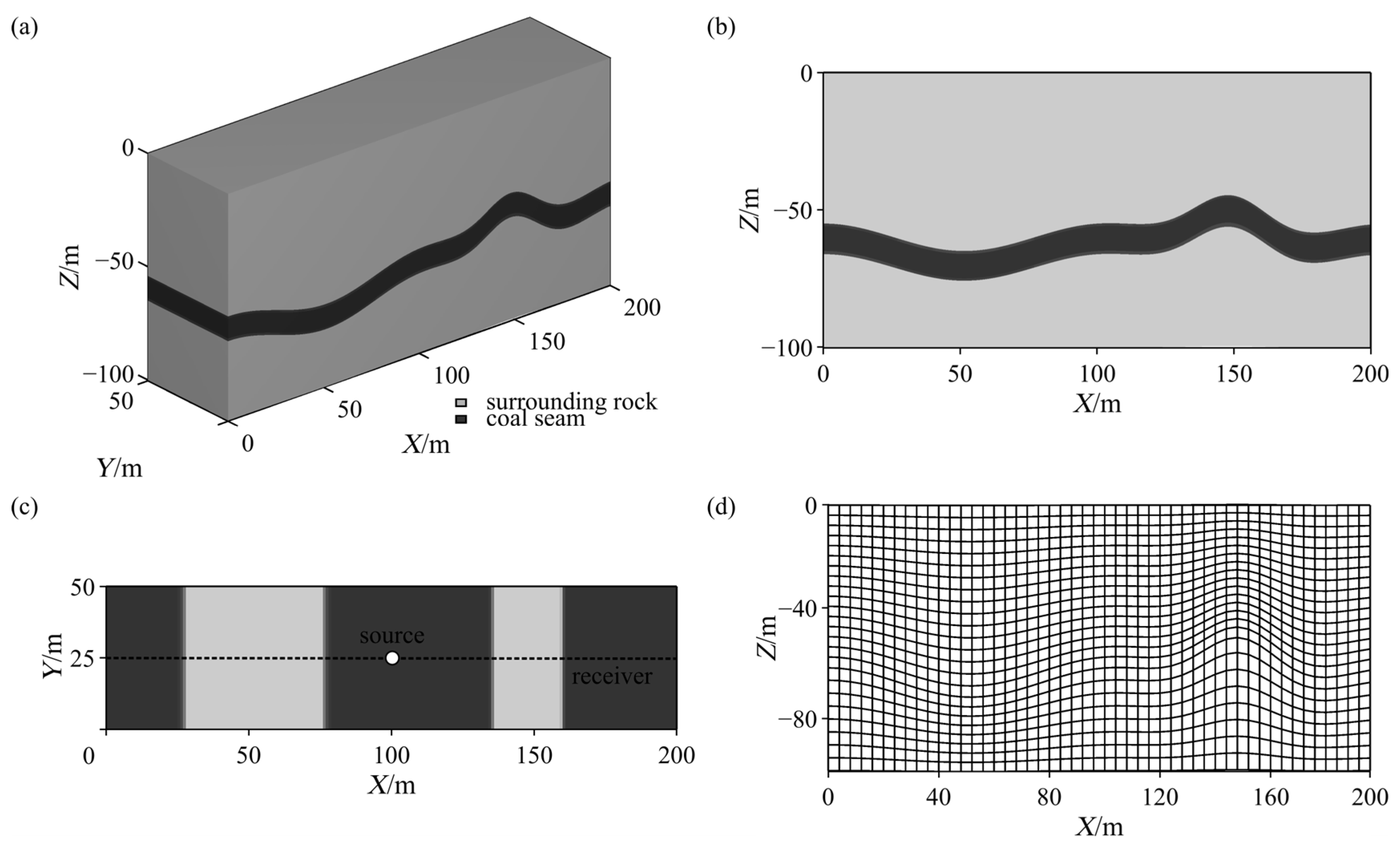
The curved coal seam model containing a fold is established with dimensions of 200 m × 50 m × 100 m corresponding to the x, y, and z directions in sequence. The coal seam is situated in the middle part, featuring a burial depth ranging from −70 m to −60 m; the roof and floor are surrounding rocks with identical lithological properties. The source is located at (100 m, 25 m, −60.034 m). The survey line is arranged in the middle of the coal seam, near y = 25 m and z = −65 m. To avoid the influence of direct wave signals, wavefield reverse-time extrapolation is implemented after removing the direct waves.

Figure 3a displays the 3D model, while Figure 3b,c present the 2D slices extracted along y = 25 m and z = −60 m, respectively. The coal seam interface is generated by superimposing the Gaussian function z₁ = h₁exp[−(x − x₀)²/a²] + z₀ and the cosine function z = z₁ + h₂cos(kx/(2πL_x)), where the parameter values are set as h₁ = 20, x₀ = 149, a = 20, z₀ = −60, h₂ = 5, k = 2, and L_x is the horizontal grid length. Figure 3d provides the curvilinear grid discretization on the slice at y = 25 m, showing that the grid conforms to the coal seam roof/floor boundaries and the fold geometry.

3.1.1. Seismograms and Snapshots

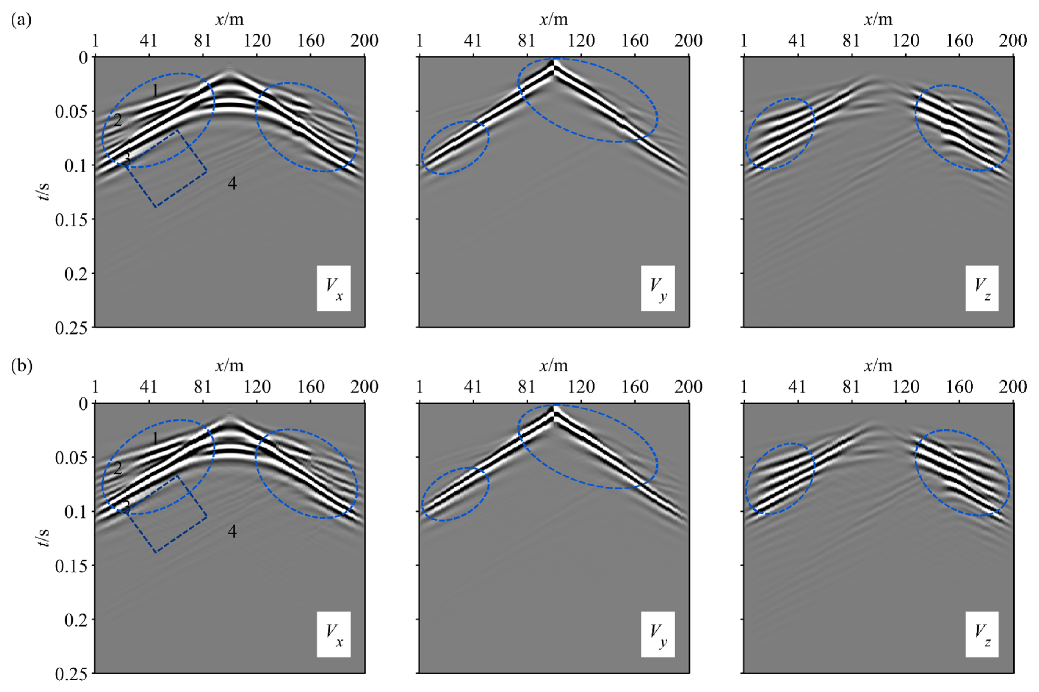
Figure 4 presents the three-component seismic records simulated using the curvilinear grid and Cartesian grid methods for the curved coal seam model containing a fold. The labeled seismic phases 1 to 4 represent the direct P-wave, direct S-wave, direct channel wave, and reflected channel wave, in that order. The numerical simulation results show that the direct channel waves are clearly visible with high energy and signal-to-noise ratio, while the reflected channel waves show comparatively low energy. The waveforms of the direct channel waves corresponding to the X and Y components are concentrated with high quality, while the direct channel wave within the Z component is relatively diffuse with scattered energy. Overall, the channel wave signals in the Y component achieve the highest quality.

In Figure 4a, the wavefield events are continuous and smooth, without obvious waveform oscillations or scattering noise. In contrast, although the overall wavefield morphology in Figure 4b is broadly similar to that of the curvilinear grid results, significant waveform discontinuities occur in the first 80 and last 80 traces (marked by blue ellipses). Moreover, spurious interface scattering induced by staircase grid discretization in the Cartesian grid system can be observed in the X-component (marked by blue rectangles). These results suggest that the curvilinear grid finite-difference method (FDM) exhibits significant advantages in 3D channel wave forward modeling in curved coal seams, effectively suppressing artificial scattering and improving wavefield simulation accuracy, and is better suited to highly undulating coal seam models.

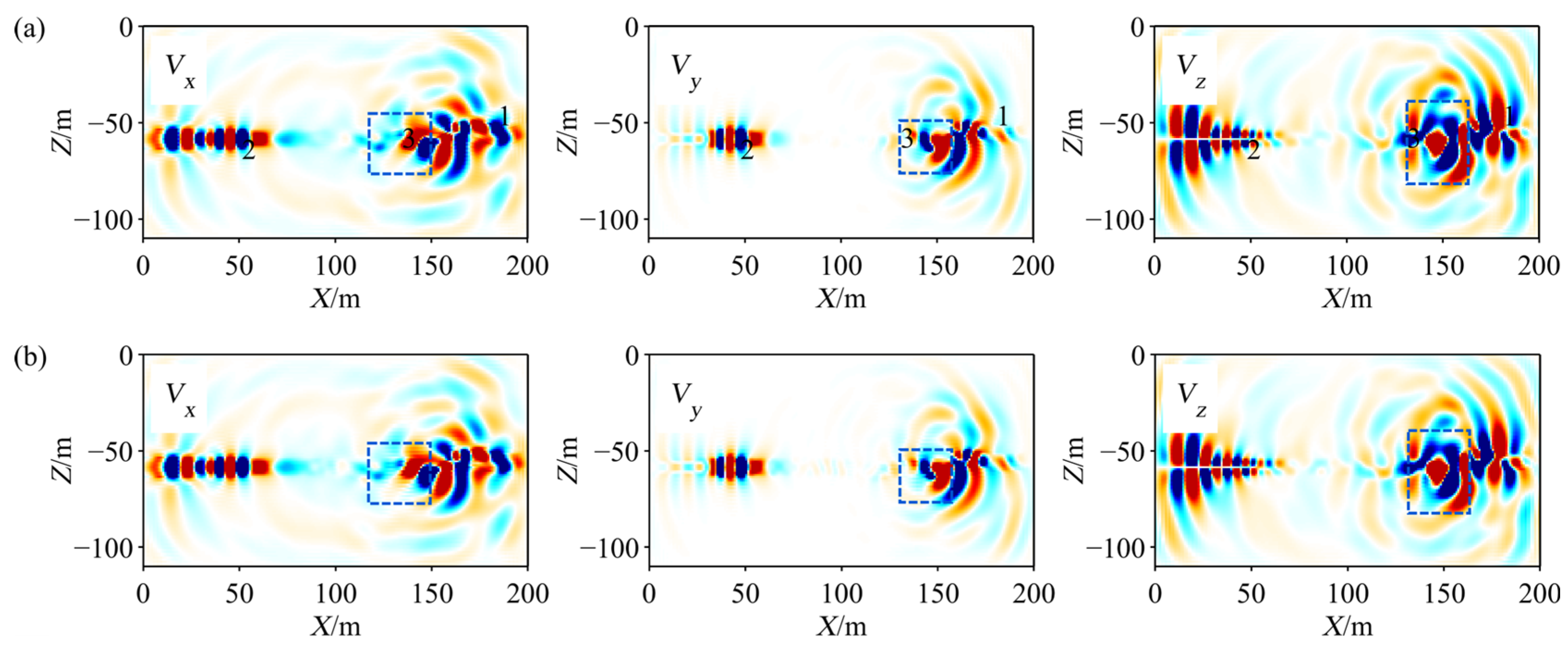
Figure 5 shows the three-component wavefield snapshots at 84 ms for the curved coal seam model containing a fold, simulated using the curved grid and Cartesian grid methods in sequence. In Figure 5a (curved grid results), the labeled wavefronts 1 to 3 represent the S wave at the coal seam roof and floor interfaces, the direct channel wave, and the reflected channel wave, respectively. It can be observed that the morphology of each wavefront is smooth and continuous, and their propagation patterns align with the geometric characteristics of the curved coal seam. Furthermore, the energy within the region outlined by the blue box exhibits good focusing, and the wavefield conforms naturally to the interfaces. The overall wavefront morphology in Figure 5b (Cartesian grid results) shows consistency with the findings in Figure 5a, but obvious local differences are present. Within the blue-boxed area, wavefront aliasing and discontinuities caused by stepped discretization can be observed. The comparison indicates that the curvilinear grid provides a more accurate representation of coal seam interfaces, resulting in more continuous channel-wave wavefronts and clearer channel-wave signals. In general, the curvilinear grid FDM exhibits higher precision for channel wave simulation of complex coal seams, which can provide a more accurate forward modeling basis for subsequent channel wave imaging or inversion.

3.1.2. RTM Imaging of Reflected Channel Waves

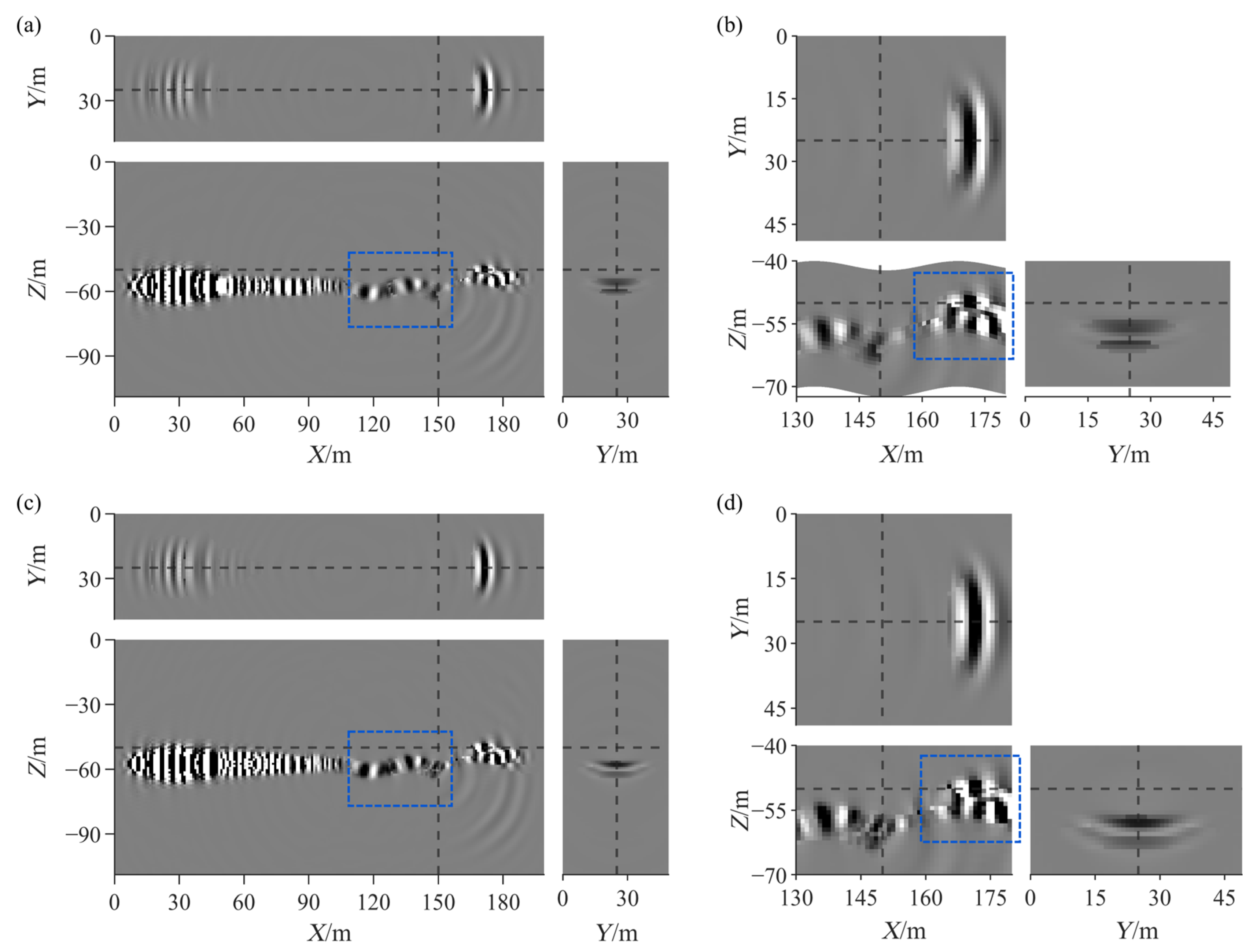
Figure 6 presents the single-shot reverse-time migration (RTM) imaging results of the curved coal seam model containing a fold, with the source located at (100 m, 25 m, −60.034 m). Overall, both the curvilinear grid and Cartesian grid methods can effectively identify the basic positions of the coal seam roof, floor, and fold structures.

However, the two grid methods exhibit significant differences in imaging accuracy and artifact suppression. Compared with the Cartesian grid results (Figure 6c), the curvilinear grid imaging (Figure 6a) achieves smoother representations at the coal seam interfaces (marked by blue rectangles), which substantially mitigates the stepped effect caused by conventional Cartesian grid discretization. The imaging outlines are more consistent with the model interfaces.

In particular, in the comparison of the locally zoomed regions (x = 130 to 180 m, y = 0 to 50 m, z = −70 to −40 m), the curvilinear grid results (Figure 6b) provide clearer and more accurate characterization of the fold structures (marked by blue rectangles), with continuous and natural reflection interfaces and effectively suppressed scattering noise. In contrast, the Cartesian grid imaging (Figure 6d) shows obvious interface jitters and scattering artifacts in the same region, which hinders the identification and interpretation of structural details. The above results indicate that, under identical simulation conditions, the curvilinear grid FDM is better able to adapt to the geometric morphology of complex coal seam interfaces enhancing the accuracy and reliability of RTM imaging for reflected channel waves.

3.2. Curved Coal Seam Model Containing a Fault

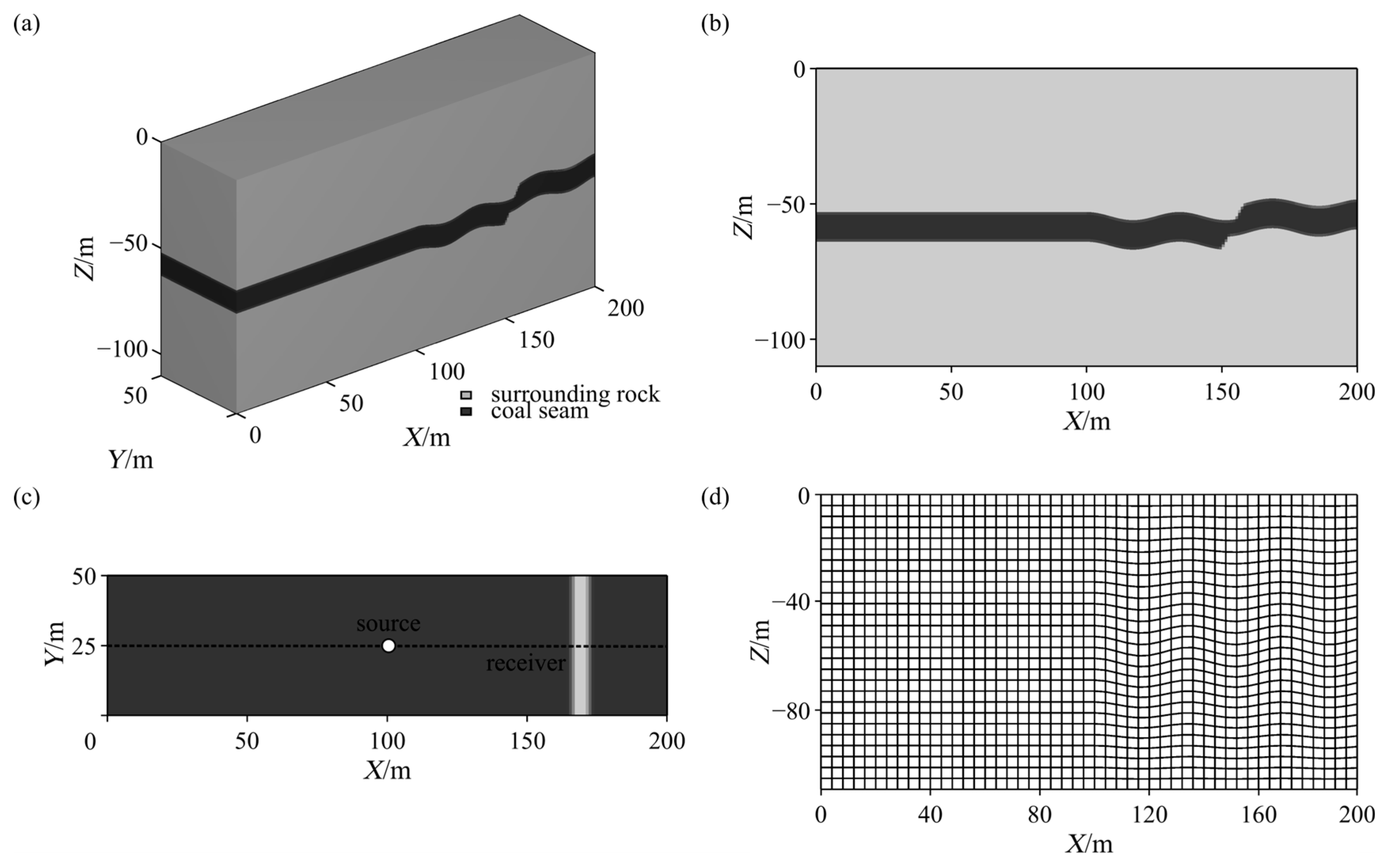
Considering that the reflected channel wave signals simulated by the model containing a fold are relatively weak, which hinders systematic analysis of their wavefield characteristics, a curved coal seam model containing a fault is constructed to enhance the reflected channel wave response and further investigate its propagation characteristics. The spatial extent of the model is 200 m × 50 m × 110 m corresponding to the x, y, and z directions in sequence. The coal seam is situated between depths of −63 m and −53 m. The source is located at (100 m, 25 m, −58 m). The survey line is deployed in the middle of the coal seam, near y = 25 m and z = −58 m.

Figure 7a shows the 3D model diagram, while Figure 7b,c present the 2D slices extracted along y = 25 m and z = −58 m, respectively. For x > 100 m, the coal seam interface is generated by the cosine function z = h cos(k₂ (x + 3)/(2πL_x1)) + z₂ − 1.5, where the parameter values are assigned as h = 1.5, k₂ = 6, L_x1 denotes the horizontal grid length, and z₂ = −63 m. To enhance the reflected channel wave response and investigate its propagation characteristics, a normal fault with a dip angle of 60° and a throw of 5 m is incorporated at x = 148 m. Figure 7d displays the schematic diagram of grid discretization for the slice at y = 25 m, which clearly demonstrates the adaptive grid variation characteristics induced by roof and floor undulation of the coal seam.

3.2.1. Seismograms and Snapshots

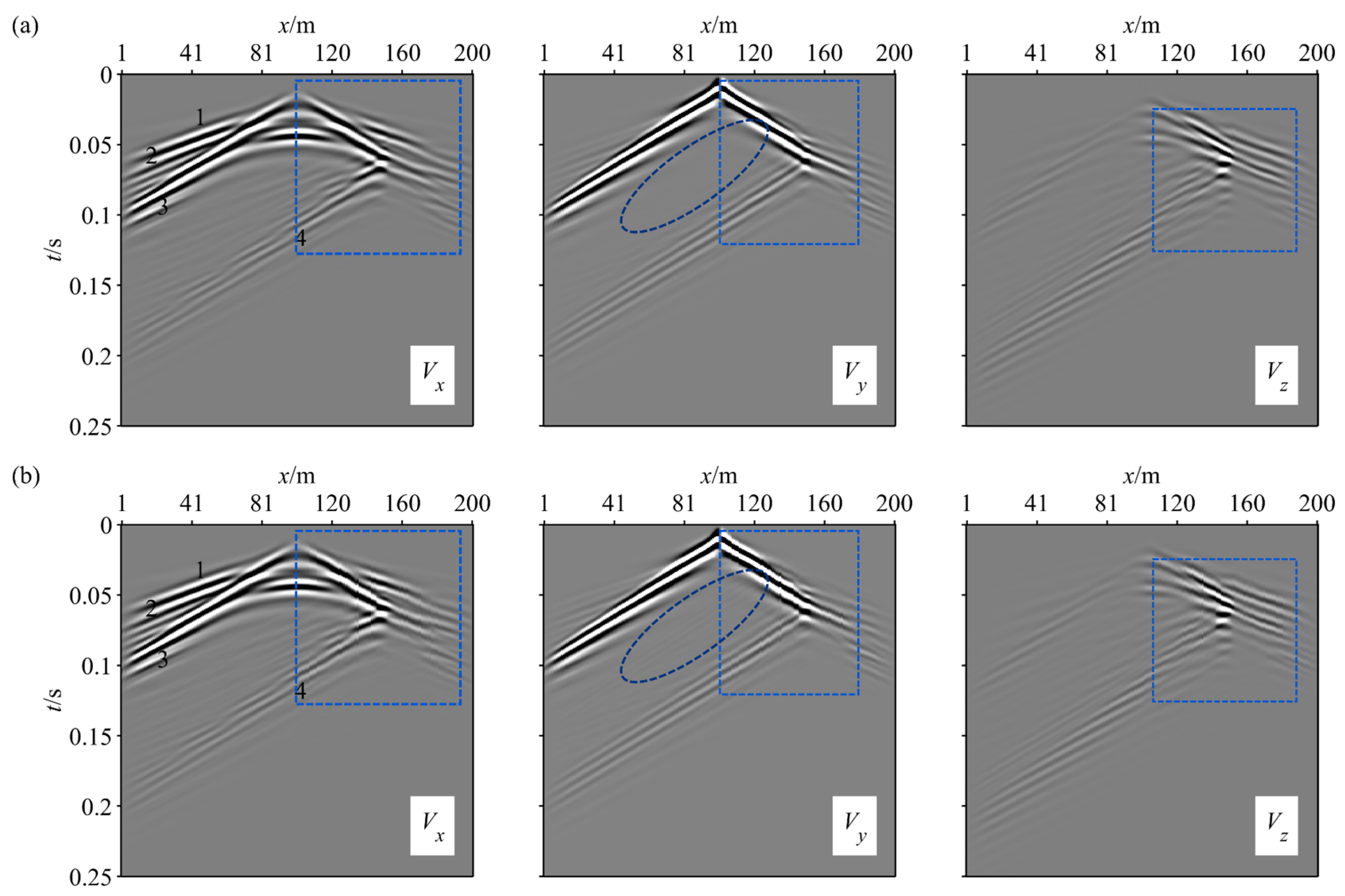
Figure 8 exhibits the three-component seismic records for the curved coal seam model containing a fault simulated using the curvilinear grid and Cartesian grid methods, respectively. The phase labeling follows that in Figure 4. The numerical simulation results indicate that both the direct and reflected channel wave signals possess high clarity and a relatively high signal-to-noise ratio. The reflected channel waves in the X and Y components exhibit favorable quality, whereas the energy of this phase in the Z component is relatively weak. Among these, the reflected channel wave signals in the Y component achieve the highest quality.

In Figure 8a (curvilinear grid results), the events of direct and reflected channel waves are continuous and smooth, without obvious scattering noise. In Figure 8b (Cartesian grid results), the overall morphology of channel waves is comparable to the curvilinear grid results. However, when the waves propagate to the irregular coal seam interface (after the 100th trace), oscillation and dislocation appear in the wavefield events (marked by blue rectangles). Especially in the Y-component, scattering artifacts are visible due to the stair-case approximation of the interface (marked by blue ellipses). Overall, the curvilinear grid results show smoother channel wave events and fewer staircase-related artifacts than the Cartesian grid results, consistent with the fold model. This method can provide a more reliable forward-modeling basis for the accurate imaging or inversion of small-scale coal seam structures using reflected or transmitted channel waves in further research.

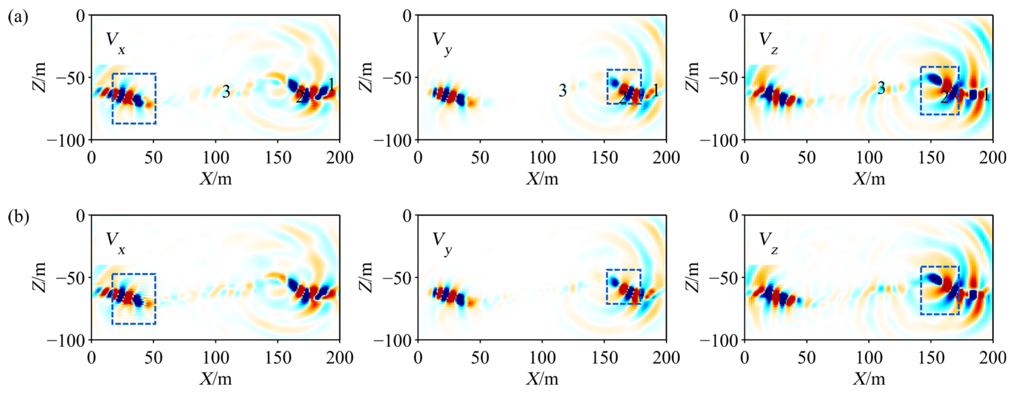
Figure 9 shows the three-component wavefield snapshots at 64 ms for the curved coal seam model containing a fault, simulated using the curved grid and Cartesian grid methods in sequence. It can be observed that the wavefront morphology is smooth and continuous, and the channel wave propagation trajectory conforms to the curved geometry of the coal seam. Additionally, pronounced energy focusing of the reflected channel wave is observed within the blue-boxed region, and the wavefield naturally conforms to the interfaces. The overall wavefield morphology in Figure 9b (Cartesian grid results) is similar to that in Figure 9a, but local differences exist. Within the blue-boxed area, slight wavefront aliasing or discontinuities are observed.

A comparison of the simulation results for the two models reveals that the reflected channel wave energy is considerably weaker in the fold model (Figure 4), yet much more pronounced in the fault model (Figure 8), particularly in the Y-component. This discrepancy can be attributed to the stronger structural discontinuities induced by the fault. Accordingly, the fault case yields clearer reflected channel wave signatures for imaging, while the fold case imposes higher requirements for suppressing spurious scattering.

3.2.2. RTM Imaging of Reflected Channel Waves

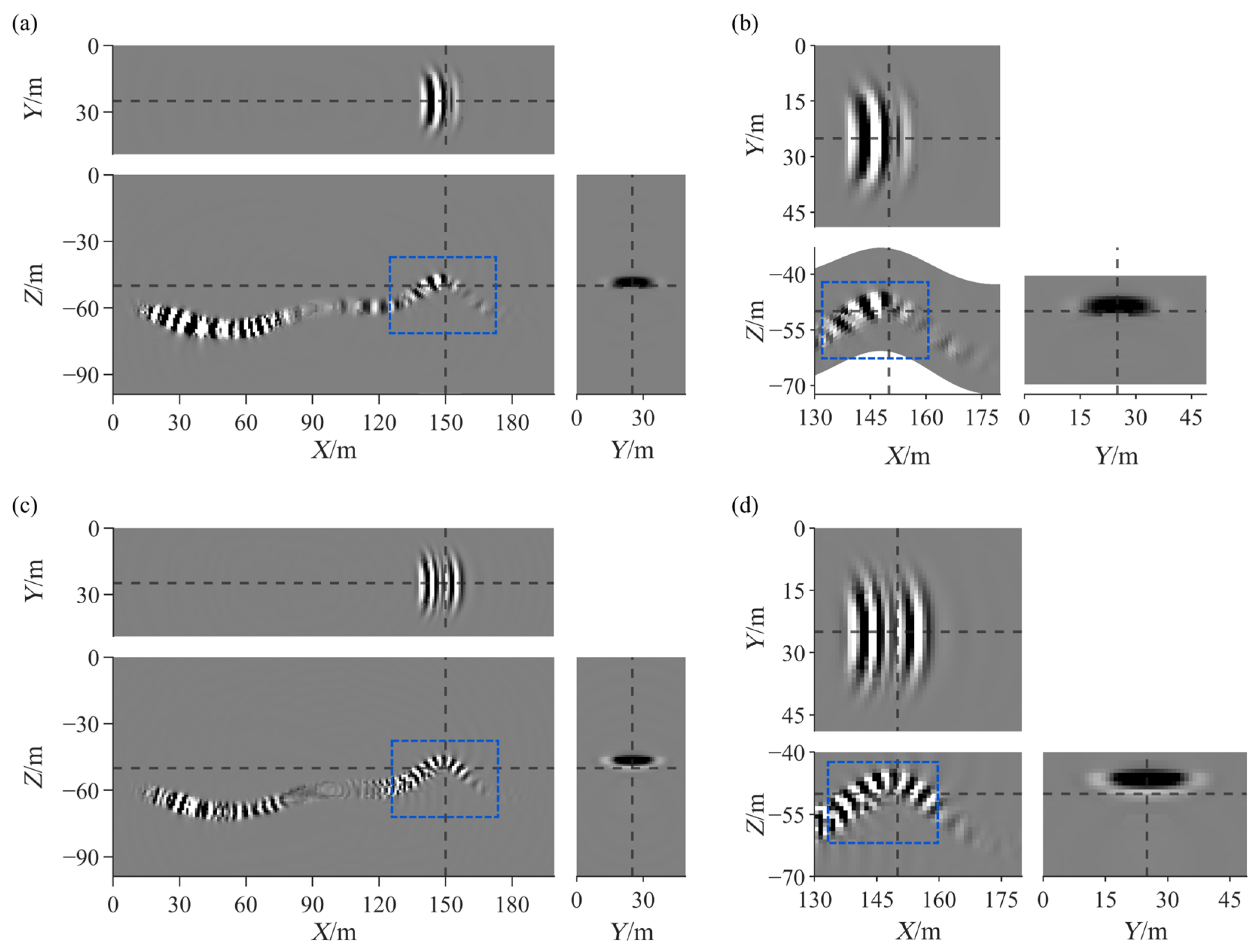
Figure 10 presents the single-shot RTM imaging results of the curved coal seam model containing a fault, where the source is situated at coordinates (100 m, 25 m, −58 m). Similar to the fold model, both grid strategies can delineate the main coal-seam interfaces and the first-order structural feature. However, the Cartesian grid imaging results (Figure 10c) exhibit staircase-related jitter and scattering near undulating interfaces, whereas the curvilinear grid imaging (Figure 10a) is smoother and more continuous, improving boundary positioning.

In particular, in the comparison of the locally zoomed regions (x = 130 to 180 m, y = 0 to 50 m, z = −70 to −40 m), the curvilinear grid results (Figure 10b) offer a more accurate depiction of the fault’s lower plate position and shape, with clear and continuous coal seam interface imaging that shows high consistency with the theoretical model. In contrast, the Cartesian grid results (Figure 10d) exhibit blurred imaging in the same region, which is unfavorable for the identification and interpretation of structural details. Overall, for highly undulating coal seam models that include folds, faults, and other structures, the FDM based on curvilinear grids, relying on its adaptive grid advantage, can more realistically simulate wavefield propagation, reduce spurious scattering caused by stair-case approximation, and thus significantly improve the precision and accuracy of RTM imaging.

A direct comparison of the RTM results indicates that the fold model focuses on reflecting the continuity and geometric accuracy of curved reflection interfaces, while the fault model places greater emphasis on the accurate imaging of fault locations and footwall boundaries. These observations suggest that, under the same simulation conditions, structural types (gradual curving vs. abrupt discontinuity) affect the imaging clarity of reflected channel waves and the geological interpretability of migration profiles.

4. Discussion

The numerical results consistently show that the curvilinear grid method produces smoother and more continuous channel wave waveforms than the conventional method. This improvement is primarily associated with interface representation: Cartesian grids approximate undulating coal seam boundaries using a staircase geometry, which introduces non-physical discontinuities and consequently generates grid-induced spurious scattering. In contrast, the curvilinear coordinate system employs body-fitted grids that conform to the coal-seam interfaces, which reduces interface-induced spurious scattering.

This benefit is also reflected in RTM imaging. The curvilinear grid method produces RTM images with better reflector continuity and fewer artifacts related to the interface. This makes it easier to see complex coal seam structures. Therefore, the core benefit of the proposed approach lies in its ability to accurately conform to the actual geological geometry, which is particularly advantageous for simulating coal seams with strong undulations.

The present work is validated using theoretical models. Extending the method to more realistic settings (e.g., stronger heterogeneity, more complex structures, and larger-scale 3D domains) will increase computational demands in memory, runtime, and data I/O for both 3D elastic modeling and RTM. Moreover, several field-relevant effects are not considered in the current verification, including 3D roadway geometry, anisotropy, and viscoelastic attenuation, which may further influence channel wave propagation and scattering characteristics. Future work will consider incorporating these factors and employing more realistic numerical models for comprehensive evaluation. To facilitate large-scale 3D applications, parallel computing and GPU acceleration will be investigated to improve computational efficiency.

5. Conclusions

This study derives the 3D elastic velocity-stress equations in a curvilinear coordinate system and develops a curvilinear grid FD framework for 3D channel wave modeling and RTM imaging. The DRP/opt MacCormack scheme and the fourth-order Runge–Kutta algorithm are employed to discretize the spatial and temporal partial derivatives, and RTM is implemented with the excitation amplitude imaging condition. Compared with conventional Cartesian grids, the proposed method better represents undulating coal seam interfaces and reduces spurious scattering induced by staircase approximation, leading to improved waveform continuity in simulations and enhanced reflector continuity with fewer artifacts in RTM images. Future work will extend the validation to more realistic large-scale models that include roadway effects, anisotropy, and viscoelastic attenuation. Additionally, parallel/GPU acceleration will be investigated for practical applications.

References

1. Wang, G.; Liu, F.; Pang, Y.; Ren, H.; Ma, Y. Coal mine intellectualization: The core technology of high quality development. J. China Coal Soc. 2019, 44, 349–357. [Google Scholar] [CrossRef]
2. Wang, G. New technological progress of coal mine intelligence and its problems. Coal Sci. Technol. 2022, 50, 1–27. [Google Scholar] [CrossRef]
3. Zhang, P.; Li, S.; Qiu, S.; Guo, L.; Hu, X. Advance detection technology and development of fast intelligent roadway drivage. J. China Coal Soc. 2021, 46, 2158–2173. [Google Scholar] [CrossRef]
4. Liu, J.; Wang, E.; Sa, Z.; Zhang, Y.; Wang, C.; Lu, S. Effects of coalbed occurrence conditions on risk of coal and gas outburst. China Saf. Sci. J. (CSSJ) 2016, 26, 98–103. [Google Scholar] [CrossRef]
5. Feng, L.; Zhang, Y.; Zhang, H.; Dong, Z. Feasibility of in-seam seismic predictionin thedeformed coal. J. Min. Saf. Eng. 2017, 34, 1027–1034. [Google Scholar] [CrossRef]
6. Zhang, P.; Ou, Y.; Li, S. Development quo-status and thinking of mine geophysical prospecting technology and equipment in China. Coal Sci. Technol. 2021, 49, 1–15. [Google Scholar] [CrossRef]
7. Liu, S.; Yu, S.; Wang, B.; Zhang, X. Study on processing method of seismic reflection wave field for advanced detection of mine gateway. Coal Sci. Technol. 2015, 43, 100–103. [Google Scholar] [CrossRef]
8. Wang, J.; Ye, H.; Zhang, G.; Li, G.; Wu, G.; Niu, H.; Yang, Y.; Guan, Q. A review on research of reflected in-seam wave detection technology in coal mine. Coal Geol. Explor. 2023, 51, 292–300. [Google Scholar] [CrossRef]
9. Korn, M.; Stockl, H. Reflection and transmission of Love channel waves at coal seam discontinuities computed with a finite difference method. J. Geophys. 1982, 50, 171–176. [Google Scholar] [CrossRef]
10. Edwards, S.; Asten, M.; Drake, L. P-SV wave scattering by coal-seam inhomogeneities. Geophysics 1985, 50, 214–223. [Google Scholar] [CrossRef]
11. Buchanan, D. The scattering of SH-channel waves by a fault in a coal seam. Geophys. Prospect. 1986, 34, 343–365. [Google Scholar] [CrossRef]
12. Krey, T.C. Channel waves as a tool of applied geophysics in coal mining. Geophysics 1963, 28, 701–714. [Google Scholar] [CrossRef]
13. Asten, M.; Drake, L.; Edwards, S. In-seam seismic Love wave scattering modeled by the finite element method. Geophys. Prospect. 1984, 32, 649–661. [Google Scholar] [CrossRef]
14. Lou, M.; Crampin, S. Dispersion of guided waves in thin anisotropic waveguides. Geophys. J. Int. 1991, 107, 545–555. [Google Scholar] [CrossRef]
15. Ji, G.; Cheng, J.; Zhu, P.; Li, H. 3-D numerical simulation and dispersion analysis of in-seam wave in underground coal mine. Chin. J. Geophys. 2012, 55, 645–654. [Google Scholar] [CrossRef]
16. Qiao, Y.; Teng, J.; Pi, J. Rayleigh channel wave field and dispersion of coal seams with small faults. Chin. J. Geophys.-Chin. Ed. 2018, 61, 4976–4987. [Google Scholar] [CrossRef]
17. Ji, G.; Wei, J.; Yang, S.; Yang, J.; Ding, R.; Zhang, G. Preliminary study on wave field and dispersion characteristics of channel waves in HTI coal seam medium. Chin. J. Geophys.-Chin. Ed. 2019, 62, 789–801. [Google Scholar] [CrossRef]
18. Jiao, W.; Ji, G.; Tang, X.; Liu, Z. Analysis of response characteristics of fault structural channel wave in viscoelastic coal seam. Saf. Coal Mines 2023, 54, 154–160. [Google Scholar] [CrossRef]
19. Wu, G. Research and application of the seismic exploration technique using reflected in-seam waves in identifying folds and faults in coal seams. Coal Geol. Explor. 2024, 52, 154–165. [Google Scholar] [CrossRef]
20. Li, Q.; Li, Z.; Huang, J.; Li, N.; Su, Z. Factor Analysis of Seismic Modeling with Topography Based on a Fully Staggered Body-Fitted Grids. J. Jilin Univ. Earth Sci. Ed. 2016, 46, 920–929. [Google Scholar] [CrossRef]
21. Kristek, J.; Moczo, P.; Galis, M. Stable discontinuous staggered grid in the finite-difference modelling of seismic motion. Geophys. J. Int. 2010, 183, 1401–1407. [Google Scholar] [CrossRef]
22. Zhang, W.; Chen, X. Traction image method for irregular free surface boundaries in finite difference seismic wave simulation. Geophys. J. Int. 2006, 167, 337–353. [Google Scholar] [CrossRef]
23. Zhang, W.; Shen, Y. Unsplit complex frequency-shifted PML implementation using auxiliary differential equations for seismic wave modeling. Geophysics 2010, 75, T141–T154. [Google Scholar] [CrossRef]
24. Zhang, W.; Zhang, Z.; Chen, X. Three-dimensional elastic wave numerical modelling in the presence of surface topography by a collocated-grid finite-difference method on curvilinear grids. Geophys. J. Int. 2012, 190, 358–378. [Google Scholar] [CrossRef]
25. Jiang, L.; Zhang, W. TTI equivalent medium parametrization method for the seismic waveform modelling of heterogeneous media with coarse grids. Geophys. J. Int. 2021, 227, 2016–2043. [Google Scholar] [CrossRef]
26. Hu, Y.; McMechan, G.A. Imaging mining hazards within coalbeds using prestack wave equation migration of in-seam seismic survey data: A feasibility study with synthetic data. J. Appl. Geophys. 2007, 63, 24–34. [Google Scholar] [CrossRef]
27. Ding, L.; Liu, Y. Progress in reverse time migration imaging. Prog. Geophys. 2011, 26, 1085–1100. [Google Scholar] [CrossRef]
28. Kong, X.; Hu, Q.; Liu, D.; Wang, W.; Yang, J.; Li, X. Research on RTM and Kirchhoff migration gathering. CT Theory Appl. 2022, 25, 507–514. [Google Scholar] [CrossRef]
29. Liu, T.; Pan, D.; Li, D.; Li, H. In-Seam Seismic Exploration; University of Mining and Technology Press: Xuzhou, China, 1994; p. 161. [Google Scholar]
30. Hixon, R.; Turkel, E. Compact implicit MacCormack-type schemes with high accuracy. J. Comput. Phys. 2000, 158, 51–70. [Google Scholar] [CrossRef]
31. Tam, C.K.; Webb, J.C. Dispersion-relation-preserving finite difference schemes for computational acoustics. J. Comput. Phys. 1993, 107, 262–281. [Google Scholar] [CrossRef]
32. Hixon, R. On increasing the accuracy of MacCormack schemes for aeroacoustic applications. In Proceedings of the 3rd AIAA/CEAS Aeroacoustics Conference, Atlanta, GA, USA, 12–14 May 1997; p. 1586. [Google Scholar]
33. Whitmore, N.D. Iterative depth migration by backward time propagation. In Proceedings of the SEG Technical Program Expanded Abstracts 1983; Society of Exploration Geophysicists: Houston, TX, USA, 1983; pp. 382–385. [Google Scholar]
34. Claerbout, J.F. Toward a unified theory of reflector mapping. Geophysics 1971, 36, 467–481. [Google Scholar] [CrossRef]
35. Chang, W.F.; McMechan, G.A. Reverse-time migration of offset vertical seismic profiling data using the excitation-time imaging condition. Geophysics 1986, 51, 67–84. [Google Scholar] [CrossRef]
36. Zhang, Z.; Liu, Y.; Xu, T.; Bai, Z. A stable excitation amplitude imaging condition for reverse time migration in elastic wave equation. Chin. J. Geophys.-Chin. Ed. 2013, 56, 3523–3533. [Google Scholar] [CrossRef]
37. Nguyen, B.D.; McMechan, G.A. Excitation amplitude imaging condition for prestack reverse-time migration. Geophysics 2013, 78, S37–S46. [Google Scholar] [CrossRef]
38. Zhang, M.; Zhou, H.; Chen, H.; Jiang, S.; Jiang, C. Reverse-time migration using local Nyquist cross-correlation imaging condition. IEEE Trans. Geosci. Remote Sens. 2022, 60, 5913914. [Google Scholar] [CrossRef]
39. Wang, J.; Li, Q.; Qiao, B.; Qi, J. Reverse time migration using excitation amplitude imaging condition based on accurate first-arrival traveltimes calculation. IEEE Trans. Geosci. Remote Sens. 2025, 63, 5903111. [Google Scholar] [CrossRef]
Figure 1. Schematic diagram for reflected in-seam wave detection.
Processes 14 00664 g001
Figure 2. Coordinate transformation between curvilinear and Cartesian grids.
Processes 14 00664 g002
Figure 3. The curved coal seam model containing a fold: (a) 3D velocity model; (b) 2D velocity model (at y = 25 m); (c) acquisition geometry (at z = −60 m); (d) schematic diagram of grid discretization (at y = 25 m).
Processes 14 00664 g003
Figure 4. Seismograms for the curved coal seam model containing a fold: (a) curvilinear grid; (b) Cartesian grid.
Processes 14 00664 g004
Figure 5. Snapshots at 84 ms for the curved coal seam model containing a fold: (a) curvilinear grid; (b) Cartesian grid.
Processes 14 00664 g005
Figure 6. RTM imaging results for the curved coal seam model containing a fold at x = 150 m, y = 25 m, and z = −50 m: (a) full imaging result of curvilinear grid; (b) local imaging result of curvilinear grid (x = 130 to 180 m, y = 0 to 50 m, z = −70 to −40 m); (c) full imaging result of Cartesian grid; (d) local imaging result of Cartesian grid (x = 130 to 180 m, y = 0 to 50 m, z = −70 to −40 m).
Processes 14 00664 g006
Figure 7. The curved coal seam model containing a fault: (a) 3D velocity model; (b) 2D velocity model (at y = 25 m); (c) acquisition geometry (at z = −58 m); (d) schematic diagram of grid discretization (at y = 25 m).
Processes 14 00664 g007
Figure 8. Seismograms for the curved coal seam model containing a fault: (a) curvilinear grid; (b) Cartesian grid.
Processes 14 00664 g008
Figure 9. Snapshots at 64 ms for the curved coal seam model containing a fault: (a) curvilinear grid; (b) Cartesian grid.
Processes 14 00664 g009
Figure 10. RTM imaging results for the curved coal seam model containing a fault at x = 150 m, y = 25 m, and z = −50 m: (a) full imaging result of curvilinear grid; (b) local imaging result of curvilinear grid (x = 130 to 180 m, y = 0 to 50 m, z = −70 to −40 m); (c) full imaging result of Cartesian grid; (d) local imaging result of Cartesian grid (x = 130 to 180 m, y = 0 to 50 m, z = −70 to −40 m).
Processes 14 00664 g010