A Data-Driven Optimization Method for Minimum-Cost Formate Brine Formulations Under Density Constraints

Abstract

Formate solutions are widely used as completion, workover, and kill fluids; however, in multisolute systems, conventional experimental approaches struggle to efficiently identify formulations that simultaneously satisfy target density requirements and minimize formulation cost. To address this challenge, a data-driven optimization framework based on regression modeling was developed to determine minimum-cost formate formulations under specified density constraints. Seven solution systems comprising sodium formate, potassium formate, and cesium formate in single-solute, binary-solute, and ternary-solute combinations were investigated at 20 °C, using 70 data sets collected from the literature and laboratory experiments. The solute-to-solvent mass ratio (SSMR) was introduced as the key formulation variable to construct solution density prediction models, and a cost-based objective function was established to inversely calculate optimal SSMR combinations. Model predictions were validated against laboratory measurements, showing mean density errors ranging from 0.022 to 0.145 g/cm³ across the seven systems, with an overall RMSE of 0.094 g/cm³ and MAE of 0.070 g/cm³. The results demonstrate that the proposed data-driven optimization method enables accurate density prediction and cost-efficient formulation design, providing a practical and scalable alternative to traditional trial-and-error experimental methods for wellbore working-fluid optimization.

1. Introduction

In petroleum engineering practice, fluid density is one of the key parameters that must be strictly controlled for drilling fluids, completion fluids, as well as workover and kill fluids. Appropriate fluid density is essential not only for maintaining wellbore pressure balance and ensuring well control safety but also for influencing wellbore stability, formation protection, and the smooth execution of field operations. Therefore, formulating working fluids with controllable density, stable performance, and minimum possible cost while satisfying engineering requirements has long been a central objective in field applications.

Completion, workover, and kill fluid systems exhibit considerable diversity and are commonly classified into solid-containing and solids-free systems according to their phase composition. In solid-containing systems, fluid density is primarily increased by introducing weighting materials, which provides a wide adjustable density range and a relatively mature application process.

The problems of weighting material sedimentation and insufficient system stability in ultra-high-density drilling fluids. Based on an ultra-high-density weighting material system, a high-solids dispersant (SMS-19) and an ultra-low-viscosity colloidal stabilizer (SML-4) were developed. A stable ultra-high-density weighted drilling fluid formulation was thus established, enabling the drilling fluid density to be increased to above 2.85 kg/L and successfully applied in drilling high-pressure intervals, thereby verifying the engineering feasibility of the proposed weighting system [1].

The insufficient high-temperature resistance and poor contamination tolerance of conventional drilling fluids by using barite to adjust density and developed a high-density saturated brine drilling fluid with a density of 2.60 g/cm³. This system met the requirements of natural gas drilling operations in three contract blocks in Turkmenistan and Uzbekistan [2].

To solve wellbore stability problems encountered during drilling through extremely thick salt–gypsum formations and directional drilling within such intervals. Based on barite, ultrafine iron ore powder was selected as an additional weighting material to establish an ultra-high-density supersaturated brine drilling fluid system, with density reaching 2.60 g/cm³ [3].

Trace amounts of surface-treated manganese–titanium mineral complexes could replace pure barite or other conventional materials as ideal weighting agents. By using these materials to adjust system density, an ultra-high-density oil-based drilling fluid system (2.35–2.65 g/cm³) was developed and successfully applied under ultra-high-temperature and high-pressure conditions [4].

Increased weighting materials to raise mud density from 1.80 g/cm³ to 2.55 g/cm³, successfully maintaining drilling-fluid stability under high-temperature and ultra-high-density conditions [5]. In the same year, Wang Guisong et al. used barite as the weighting material to formulate a high-density kill fluid with a density above 1.60 g/cm³, demonstrating good field performance [6].

Excessive solid content increases the likelihood of solid particles invading the formation, causing plugging and contamination. When the solid concentration exceeds the suspension capacity of the liquid phase, particle agglomeration and sedimentation may occur, resulting in density non-uniformity and degraded rheological and flow properties of the kill fluid. Consequently, kill fluid systems have gradually shifted toward solids-free formulations. In such systems, inorganic salt brines, including sodium chloride, calcium chloride, and sodium bromide solutions, are widely used due to their adjustable density and ease of formulation.

Formulated a high-density, low-damage kill fluid with a density of 1.20–1.50 g/cm³ in the Gudong area of Shengli Oilfield. Calcium chloride was also used as the density regulator, which effectively improved sand control efficiency and single-well productivity [7].

In addition, some systems regulate solution density through chemical additives. The density adjustment in such systems is continuous and controllable, allowing fine-tuned formulation design by varying additive dosage, thereby enabling better matching with formation pressure windows.

Developed a novel low-damage kill fluid using powdered polyacrylamide as a viscosifier and trivalent organic chromium ions as a crosslinking agent. The fluid density was adjustable within the range of 1.0–2.2 g/cm³. The gel exhibited minimal formation damage and could be degraded by strong oxidants. Statistical results showed that after applying the gel-type workover fluid, oil well productivity recovered on average 6–8 days earlier, and the initial water cut after operations was reduced by approximately 20% [8].

In 2013, Li Meng et al. Investigated high-temperature-resistant, high-density kill fluid systems formulated with various chemical additives to address the poor temperature tolerance and severe formation damage associated with commonly used kill fluids in oilfields. The developed system had a density of 1.85 g/cm³, and its viscosity remained below 110 mPa·s before and after exposure to 242 °C, while the API fluid loss was maintained below 8.0 mL [9].

To address complex drilling conditions in fragile formations prone to collapse and severe losses, which require timely and effective borehole strengthening. Two borehole-strengthening agents were introduced into the drilling fluid, allowing field-controllable densities in the low-density range of 1.14–1.50 g/cm³. The developed drilling fluid system successfully reconciled the contradiction between wellbore stability and low pressure-bearing capacity [10].

Severe losses during workover operations caused by insufficient formation energy and low formation pressure. A composite foam gel workover fluid system was developed using acrylamide copolymers as temporary plugging agents, chromium acetate as a crosslinker, and additional foaming and foam-stabilizing agents. The density of the workover fluid could be adjusted within the range of 1.0–1.25 g/cm³ [11].

Optimized high-density oil-based drilling fluid formulations by employing new treating agents and optimizing the particle size distribution of solids to reduce fluid density. Field tests demonstrated that the combination of managed pressure drilling and density reduction during horizontal drilling operations effectively reduced downhole complexity, increased rate of penetration, lowered overall drilling costs [12].

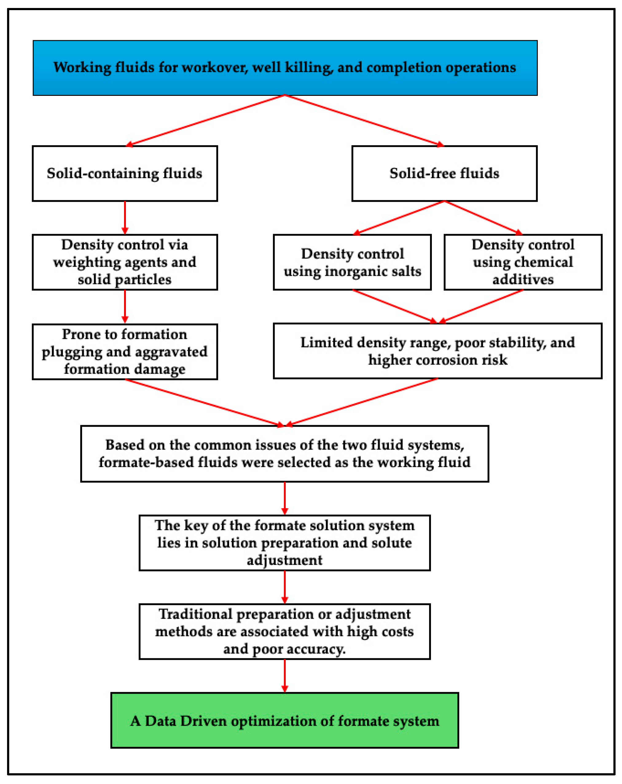
To more intuitively illustrate the research approach, a flowchart of the investigation process was drawn, as shown in Figure 1.

As shown in Figure 1, with increasingly stringent requirements for drilling fluids, higher-performance organic salt solutions are gradually selected as the base fluid. Among them, formate-based organic salts exhibit superior performance compared with conventional inorganic salt brines in terms of density regulation, thermal stability, material compatibility, and environmental friendliness. In addition, formate brines feature low corrosivity, and their clear solutions maintain good rheological properties even at high concentrations [13]. As a result, formate brines have gradually become an important development direction for solids-free kill fluid systems.

Overall, existing studies mainly rely on conventional experimental approaches for fluid formulation design, which involve considerable subjectivity and uncertainty. Methods such as full-factorial experiments, orthogonal design, and empirical formulation face inherent limitations, including a large number of possible combinations, difficulty in capturing interactions among variables, and insufficient consideration of cost factors. These limitations become particularly pronounced in formate-based systems, where density optimization depends on the formulation of the formate brine base fluid and multiple formate salts are often blended to achieve a wide adjustable density range. While single-solute systems still require extensive preliminary measurements, multisolute systems are characterized by numerous formulation combinations corresponding to a given target density, each associated with different costs. As a result, exhaustive experimental exploration is impractical, leading to high experimental costs and making it difficult for traditional approaches to rapidly identify minimum-cost formulations that satisfy field density requirements.

To address the limitations of conventional experimental approaches, formulation design can be reformulated as a constrained optimization problem oriented toward target values. By integrating density constraints with a cost-based objective function, mathematical optimization methods provide a systematic pathway for identifying economically efficient formulations.

Develop the Pitzer model to overcome the low-concentration limitations of existing electrolyte theories. By extending Debye–Hückel theory with ionic-strength-dependent virial coefficients to account for short-range interactions, the model provides accurate thermodynamic predictions up to several molal (typically about 3–6 mol·kg⁻¹), while retaining relatively simple equations and good agreement with experimental data for both single and mixed electrolytes [14].

Develop the electrolyte NRTL (eNRTL) model to address the difficulty of describing excess Gibbs energy over a wide composition range. By decomposing the excess Gibbs energy into long-range electrostatic and short-range local-composition contributions, the model successfully represents systems from molecular liquids to fused salts [15].

Develop a SAFT-type equation of state to model associating liquids by extending Wertheim’s theory. By decomposing the Helmholtz energy into Lennard–Jones, chain, and association contributions, the model accurately reproduces molecular simulation results and experimental phase equilibrium data for selected pure compounds [16].

Addressed the limitation that coalbed methane production studies mainly focused on geological factors while neglecting engineering parameters. By considering engineering stages such as drilling and completion, hydraulic fracturing, and production drainage, they applied grey relational analysis and correlation analysis to establish a data-driven mathematical model relating production to engineering parameters. The results were consistent with field performance, demonstrating the feasibility of the proposed approach [17].

Proposed a predictive method combining intelligent optimization algorithms with neural networks to address the lack of a general density prediction model for drilling fluids under high-temperature and high-pressure downhole conditions. By training the model with existing experimental data, high-accuracy density prediction was achieved. Compared with other intelligent methods, the proposed model demonstrated superior accuracy and stability, showing good engineering adaptability and application potential [18].

Proposed an adaptive model combining extreme learning machines and the k-nearest neighbors algorithm to predict the density of oil-based drilling fluids under high-temperature and high-pressure conditions. Trained on experimental data, the model achieved fast learning speed, strong generalization ability, and higher prediction accuracy than conventional models, effectively overcoming limitations such as local optima and low training efficiency [19].

Proposed an improved recurrent neural network algorithm to address issues of low efficiency, insufficient accuracy, and poor adaptability in petroleum engineering data-driven classification. By introducing rectified linear unit activation functions, multilayer network structures, and adaptive optimization strategies, the stability and classification accuracy of model training were enhanced. Experimental results demonstrated that the proposed method achieved high accuracy and good practical value across multiple application domains [20].

Well-established thermodynamic models, such as the Pitzer model, eNRTL model, and SAFT-type equations of state, provide physically rigorous descriptions of electrolyte and associating fluid systems, but their application requires strictly satisfied assumptions, detailed system-specific interaction parameters, and extensive calibration. In practical formulation problems, these conditions are often difficult to meet, which significantly limits their applicability and feasibility in engineering optimization. Likewise, machine-learning-based models, including neural networks and support vector machines, rely heavily on large, representative, and high-quality datasets to achieve reliable performance. Such data requirements are rarely fulfilled in field-oriented formulation studies, thereby restricting their practical applicability. When the target density is known, accurately predicting and selecting component proportions depends on identifying and quantifying the relationships among variables. Under these constraints, regression analysis offers transparent modeling procedures, clear physical meaning, and high computational efficiency, and is particularly suitable for engineering problems with well-defined variables and limited sample sizes. Therefore, regression-based analysis is adopted in this study as a feasible and effective optimization approach under specified performance and cost constraints.

Addressed the problems of dosage determination and cost optimization of organic salt solutions under different density requirements. Based on laboratory density data obtained for both single-salt and blended systems, nonlinear multivariate least squares and optimization theory were employed to establish mathematical relationships and optimization models between solution density and dosage. The results demonstrated high model accuracy, enabling the determination of optimal dosages for arbitrary target densities, and showing strong engineering applicability [21].

Conducted laboratory experiments to address cost control while maintaining the performance of oil and gas well working fluids. The relationships between additive dosage and fluid performance under two treatment agents were determined. By combining nonlinear multivariate least squares with optimization theory, mathematical expressions and optimization models were established. Multiple field applications verified the effectiveness of the method in cost control, yielding significant economic benefits [22].

Addressed the difficulty of optimizing plastic viscosity in microbubble drilling fluids and the limitations of traditional orthogonal and uniform experimental designs, such as uncertain reagent dosage and unsatisfactory results. A multivariate regression experimental approach was adopted, in which 17 formulations were designed and viscosity was measured to establish a quadratic regression model. The results showed that the method achieved high accuracy with prediction errors below 5%, effectively optimizing the plastic viscosity of microbubble drilling fluids and demonstrating practical applicability [23].

Investigated the rheological properties of oil-based drilling fluids with typical formulations under high-temperature and high-pressure conditions. Through multivariate nonlinear regression analysis of experimental data, mathematical models were established to predict apparent viscosity, plastic viscosity, and yield stress under high-temperature and high-pressure conditions. The predicted values showed good agreement with measured data, with correlation coefficients exceeding 0.98 [24].

Established mathematical relationships between conventional logging data and permeability, invasion radius, and skin factor based on intermediate parameters such as median grain size, porosity, and resistivity, providing a methodological basis for quantitatively evaluating formation damage using logging data [25].

Developed a model-based optimization method for drilling fluid density and viscosity to balance wellbore stability, pressure control, and hole-cleaning efficiency. Based on regression models embedded in wellbore hydraulics simulation software, the method can calculate optimal drilling fluid density, viscosity, and related drilling parameters (such as flow rate and rate of penetration) within seconds while satisfying downhole pressure and operational constraints. By defining different objective functions, such as minimum pressure loss, maximum cutting transport efficiency, or cost functions, the method enables flexible optimization for various geological and operational conditions, significantly improving the accuracy and efficiency of density control. This approach is suitable for automated drilling fluid management systems and enhances drilling safety and economic performance [26].

Investigated the unclear causes of sudden production decline during the trial production period of Well SHB-X in the Shunbei Oilfield. Reservoir sensitivity experiments and drilling fluid compatibility evaluations indicated that velocity sensitivity, salt sensitivity, and drilling fluid damage were insufficient to cause production shutdown. Subsequently, based on 100 days of production data from seven wells in the same block, data-driven methods were applied to quantitatively analyze the relationship between liquid productivity index and 12 influencing factors. The results showed that wax deposition and asphaltene precipitation induced by large well depth and high production rates were the primary plugging mechanisms. Field analysis demonstrated that controlling daily liquid production is key to maintaining stable production in deep carbonate reservoirs [27].

Conducted experimental studies on different types of drilling fluids and improved the temperature–pressure correction model provided by API standards by introducing a quadratic temperature term to account for the nonlinear influence of temperature on drilling fluid liquid-phase density. Comparative analysis with experimental data showed that the improved model consistently outperformed the API model in density prediction accuracy [28].

Addressed the difficulty of using conventional skin factor to quantitatively reflect the relationship between drilling fluid properties and formation damage and its limitations in guiding field optimization. A multiparameter formation damage model based on data-driven methods was developed. Using data from nine wells drilled with velvet-type drilling fluids and six neighboring wells, multivariate regression and peeling algorithms identified apparent viscosity, density, dynamic–plastic ratio, and pH value as the main influencing factors, and quantitatively established their relationships with daily production differences. After optimizing the drilling fluid formulation for Well Yan 5-V1, daily gas production increased by nearly 800 m³. Field applications demonstrated that the method can accurately identify damage factors and provide a solid theoretical basis for drilling fluid optimization, with strong potential for wider application [29].

Prepared four oil-based drilling fluids with identical components but different densities based on field formulations and investigated the effects of temperature and pressure on drilling fluid density. A binary regression mathematical model incorporating temperature and pressure was established. Field drilling fluids of different densities were used to validate the model, and the results showed strong agreement between predicted and measured values, with an average prediction accuracy of 97.93%, meeting field application requirements [30].

To precisely guide drilling fluid density adjustment under underbalanced drilling conditions. By analyzing logging response characteristics of gas wells in buried-hill formations, a logging-parameter-based real-time drilling fluid density adjustment method was proposed. From a statistical perspective, the correlation between bottom-hole pressure difference and gas-logging parameters was analyzed, and a drilling fluid density adjustment model for the Caofeidian M structure was established, enabling timely and accurate density control during drilling operations [31].

In petroleum engineering, regression analysis and data-driven approaches have been widely applied to a range of problems, demonstrating that when system variables are well defined and experimental data are limited, data-driven modeling can provide efficient and reliable solutions for complex engineering problems. Motivated by these successful applications, the present study extends data-driven methodology to the formulation design and density optimization of working fluids by building upon the work of Ref. [31]. Their study adopted a fundamental modeling framework describing the relationship between solution density and component dosage and, although limited to binary-solute systems and mathematical relationships between solute and solvent dosages, demonstrated the feasibility of data-driven density optimization as an early application of this methodology in formulation design. On this basis, the present work further extends the approach to more complex ternary-solute systems, enabling higher-dimensional formulation optimization, and introduces a cost objective function to explicitly incorporate economic considerations, thereby achieving simultaneous satisfaction of density requirements and cost minimization [32].

All experimental measurements were conducted at a constant temperature of 20 °C. In this study, temperature was treated as a fixed condition rather than an independent variable, in order to isolate the effects of formulation composition on solution density and cost. As a result, temperature effects were implicitly embedded in the measured data and not explicitly modeled. The proposed framework is therefore applicable to formulation optimization under ambient-temperature conditions, while extension to elevated-temperature environments would require additional temperature-dependent data.

2. Materials and Methods

The implementation of minimum-cost formate brine formulations under density constraints relies on two major components. The first component involves the collection and organization of density-related data for formate solutions, including both literature review and experimental measurements. The experiments encompass the preparation of formate solutions, relevant materials, and laboratory instruments. The second component concerns the development of predictive models, including the construction of a density prediction model for formate solutions and the application of data-driven inverse calculation methods for formulation optimization.

2.1. Data Acquisition of Formate Solutions

The density–concentration relationships of single-solute solutions are well documented in the literature; therefore, density data for sodium, potassium, and cesium formate solutions were obtained directly from published sources, with 10 data sets collected for each solute.

For data unavailable in the literature, four multi-solute formate brine systems were prepared and measured in the laboratory. A total of 40 experiments were designed. The 40 laboratory experiments were designed to provide a quasi-uniform coverage of the feasible formulation space under practical solubility and operability constraints. Experimental points were systematically distributed across single-, binary-, and ternary-solute systems rather than randomly selected. The experimental design, materials, apparatus, and procedures are detailed as follows.

(1)

Experimental Design

Multi-solute formate brine solutions were prepared in the laboratory. Three binary systems composed of sodium formate (Macklin Biochemical Co., Ltd., Shanghai, China), potassium formate (Macklin Biochemical Co., Ltd., Shanghai, China), and cesium formate (Macklin Biochemical Co., Ltd., Shanghai, China), along with one ternary system, were investigated, giving a total of four solution systems. For each system, 10 experiments were conducted, resulting in 40 experiments overall. The experimental variables were solute type and solute dosage, while temperature, pressure, and humidity were controlled. During preparation, solute and solvent dosages were recorded, and solution densities were measured after completion.

(2)

Experimental Materials

Four types of formate brine solutions were prepared in the laboratory. The required materials included sodium formate (CHNaO₂; AR, 99.5%; MW, 68.01), potassium formate (CHOK; AR, 98%; MW, 84.12), and cesium formate (CHO₂Cs·H₂O; AR, 97%; MW, 195.94).

(3)

Experimental Apparatus

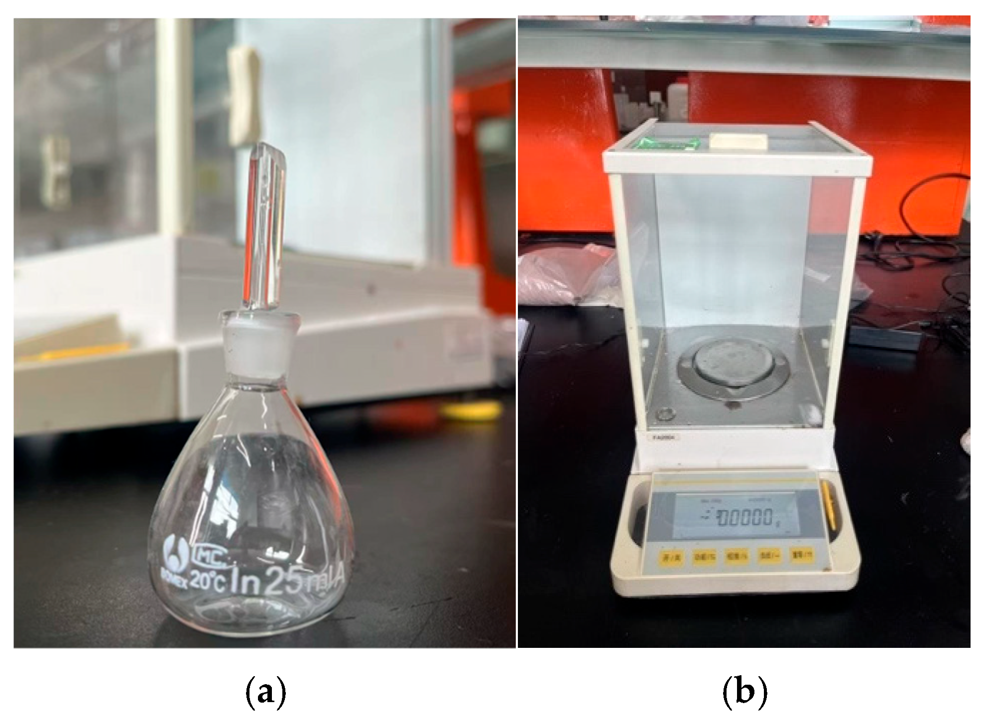
The laboratory preparation of the four formate brine solutions required basic apparatus and consumables, including beakers, graduated cylinders, spoons, weighing paper, and glass rods. Additionally, a Lee’s density bottle (standard volume 25 mL) and an analytical balance with 0.0001 g precision were used, as shown in Figure 2.

As shown in Figure 2, the pycnometer is of high-precision grade (A) and calibrated as a 25 mL “To Contain” (TC) standard at 20 °C, meaning that the liquid is filled to the graduation line at 20 °C to reach 25 mL. In practice, its actual usage precision may be lower than the nominal standard. The ten-thousandth-gram precision balance, as the name suggests, has a weighing accuracy of 0.0001 g, suitable for measuring samples that require high-precision mass data, such as chemical reagents, pycnometer mass, and solution mass.

(4)

Experimental Procedure

Measure the density of the formate solution using the pycnometer. First, add 100 mL of water to a beaker, the density of water is $\mathrm{\rho }$₀ Then add the formate powder and stir with a glass rod. If the powder does not fully dissolve, add more water and continue stirring until the powder is completely dissolved, completing the preparation of the formate solution. Rinse the pycnometer (including the glass stopper) with deionized water and dry it. Weigh the empty pycnometer on the ten-thousandth-gram precision balance to obtain mass m₀. Fill the pycnometer with deionized water up to the graduation line, slowly pouring in to avoid air bubbles. Insert the glass stopper, wipe the exterior of the pycnometer to remove water, and weigh the filled pycnometer to obtain total mass m₁. Pour out the water and dry the pycnometer. Then, pour the prepared formate solution from the beaker into the pycnometer up to the graduation line, slowly to prevent air bubbles. Insert the glass stopper, wipe the exterior to remove any liquid, and weigh the filled pycnometer to obtain total mass m₂.

Calculate the solution density using the formula. The formula for the solution density is shown in Equation (1).

$$\mathrm{\rho }={\displaystyle \frac{{\mathrm{m}}_2-{\mathrm{m}}_0}{{\mathrm{m}}_1-{ \mathrm{m}}_0}} \cdot {\mathrm{\rho }}_0$$

(1)

2.2. Definition of Solute-to-Solvent Mass Ratio

The density of a solution can be regarded as the ratio of the total mass of all components to the total volume of all components minus the volume contraction. It can be approximately calculated using Equation (2).

$$\mathrm{\rho }={\displaystyle \frac{\mathrm{m}}{\mathrm{V}}}={\displaystyle \frac{{\mathrm{m}}_{\mathrm{w}1}+{\mathrm{m}}_{\mathrm{w}2}+\cdots +{\mathrm{m}}_{\mathrm{s}}}{{\mathrm{V}}_{\mathrm{w}1}+{\mathrm{V}}_{\mathrm{w}2}+\cdots +{ \mathrm{V}}_{\mathrm{s}}-\mathrm{x}}}$$

(2)

In Equation (2), m_s is the mass of the solvent, g; m_wi is the mass of each solute, g; V_s is the volume of the solvent, mL; x is the quantified value of the volume contraction that occurs when solute and solvent are mixed, mL, Under specific environmental conditions, for a solution with a particular solute and solvent, the solution density depends only on the masses of the solute and solvent; therefore, x is a function of the solute and solvent masses.

By converting the volume of each component in the denominator of Equation (2) into the ratio of mass to density and then dividing both the numerator and denominator by m_s, Equation (3) can be obtained after simplification.

$$\mathrm{\rho }={\displaystyle \frac{{\mathrm{\alpha }}_{{\mathrm{w}}_1}+{\mathrm{\alpha }}_{{\mathrm{w}}_2}+\cdots +1}{\frac{{\mathrm{\alpha }}_{{\mathrm{w}}_1}}{{\mathrm{\rho }}_{{\mathrm{w}}_1}}+\frac{{\mathrm{\alpha }}_{{\mathrm{w}}_2}}{{\mathrm{\rho }}_{{\mathrm{w}}_2}}+\cdots +\frac{1}{{\mathrm{\rho }}_{\mathrm{s}}}-\frac{\mathrm{x}}{{\mathrm{m}}_{\mathrm{s}}}}}$$

(3)

In Equation (3), $\mathrm{\rho }$_wi is the density of the solute, $\mathrm{\rho }$_s is the density of the solvent, g/cm³; and α = m_wi/m_s, α is the mass ratio of each solute to the solvent, dimensionless.

The solute-to-solvent mass ratio (SSMR) is defined as the ratio of the solute mass to the solvent mass in a given solution. SSMR is a dimensionless ratio. It should be noted that using the SSMR does not change the actual physical significance of the solute and solvent quantities; it is essentially a measure of how much solute and solvent are present. Moreover, the SSMR is only used to quantify the relative amounts of each component in a specific solution (with fixed solute and solvent types), and its effect on density is meaningful only when comparing within the same type of solution. The solution density is a function of either the SSMR or the solute mass fraction. The following will demonstrate this using SSMR as an example.

Suppose there are two solutions composed of the same solute and solvent, and the SSMR in both solutions is identical. Their densities are $\mathrm{\rho }$₁ and $\mathrm{\rho }$₂, and their solution masses are m₁ and m₂, respectively. Due to solution homogeneity and mass conservation, the density of the same type of solution remains unchanged after mixing, and similarly, the density remains unchanged if the solution is divided arbitrarily. Therefore, even if the solution masses differ, it is always possible, through a finite number of divisions, to split the two solutions into multiple portions of equal mass. During this division process, both the density and SSMR remain unchanged. Ultimately, two sets of solutions with equal mass, identical SSMR, and densities $\mathrm{\rho }$₁ and $\mathrm{\rho }$₂ are obtained. Comparing any one portion from each set, the two solutions have equal mass and equal SSMR, which implies equal solute and solvent masses. Consequently, the densities of the two solutions must be equal, i.e., $\mathrm{\rho }$₁ = $\mathrm{\rho }$₂.

In the above comparison, the physical meanings of solute mass fraction and SSMR are generally similar. Mathematically, solute mass fraction and SSMR can be converted into each other. The relationship between solute mass fraction and SSMR is shown in Equation (4).

$${\mathrm{w}}_{\mathrm{i}}={\displaystyle \frac{{\mathrm{\alpha }}_{\mathrm{i}}}{(1+{\mathrm{\alpha }}_{\mathrm{i}})}}$$

(4)

In Equation (4), w_i is the solute mass fraction, dimensionless; α_i is the solute SSMR, dimensionless.

Solute content in solutions is commonly expressed using mass fraction or molar concentration. In this study, the model is established based on the preparation of 1 m³ of formate brine, for which the system volume is fixed during model development, allowing both descriptors to be theoretically applicable. However, during the prediction stage, solution density is the unknown target variable, and the total mass of the system cannot be determined a priori, rendering solute mass fractions impractical for prediction. In contrast, molar concentration is defined on a per-unit-volume basis and remains independent of solution density, making it applicable even when density is unknown. Nevertheless, in engineering practice, formulation design and cost evaluation are typically based on mass rather than molar quantities. Therefore, SSMR was selected as the independent variable in this study.

2.3. Establishment of Formic Salt Solution Density Model and Reverse Calculation Method for Minimum-Cost Formulation

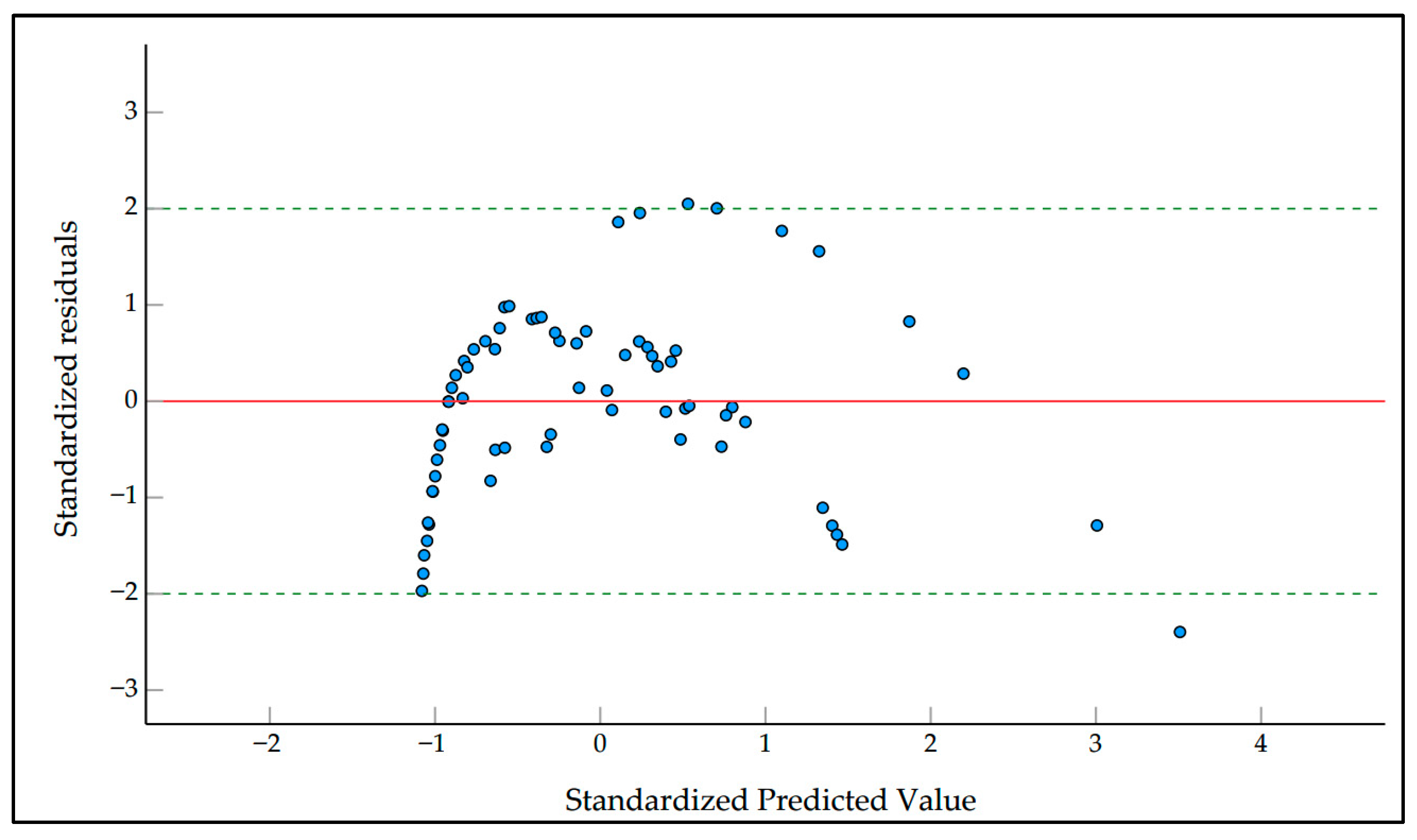
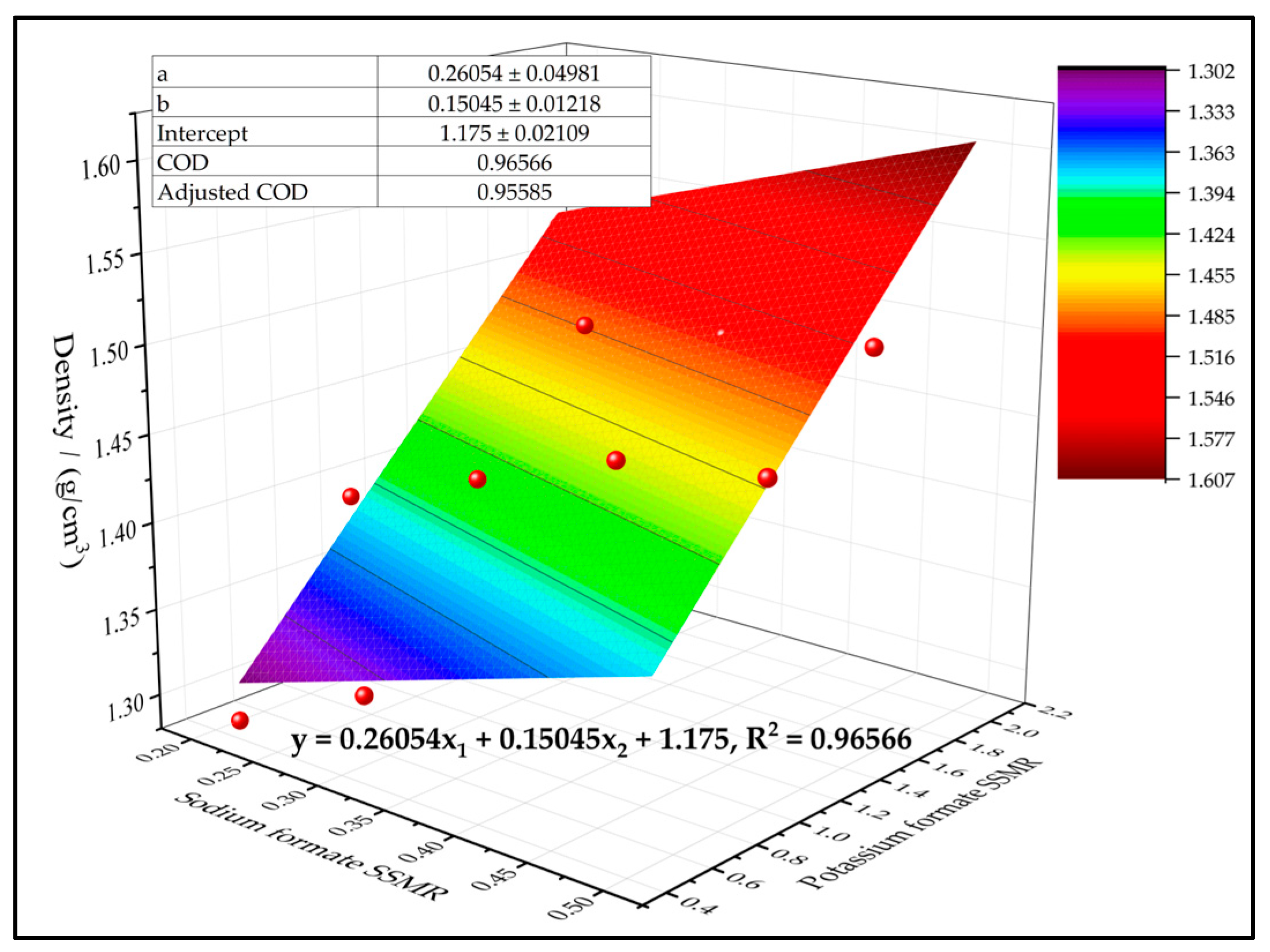
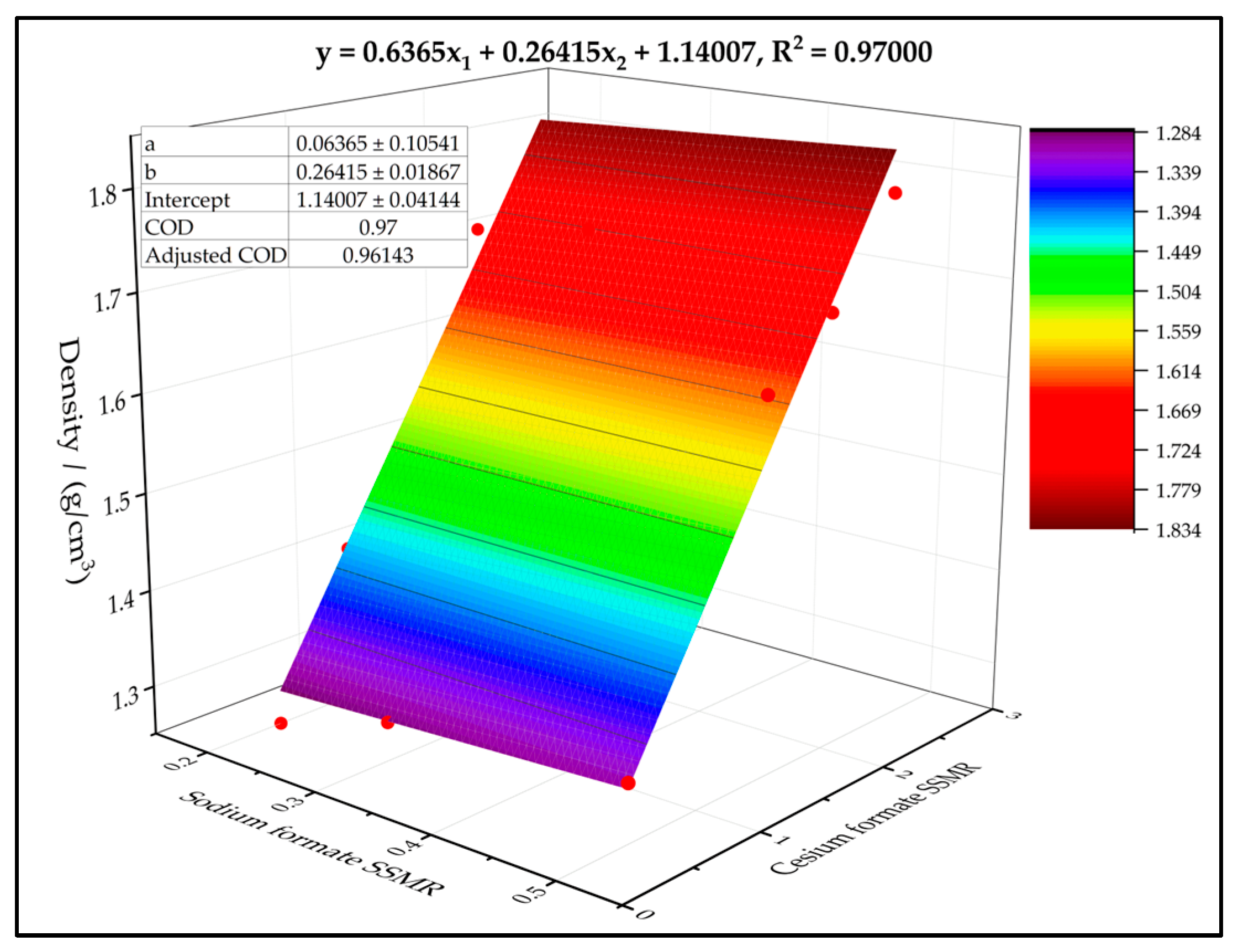
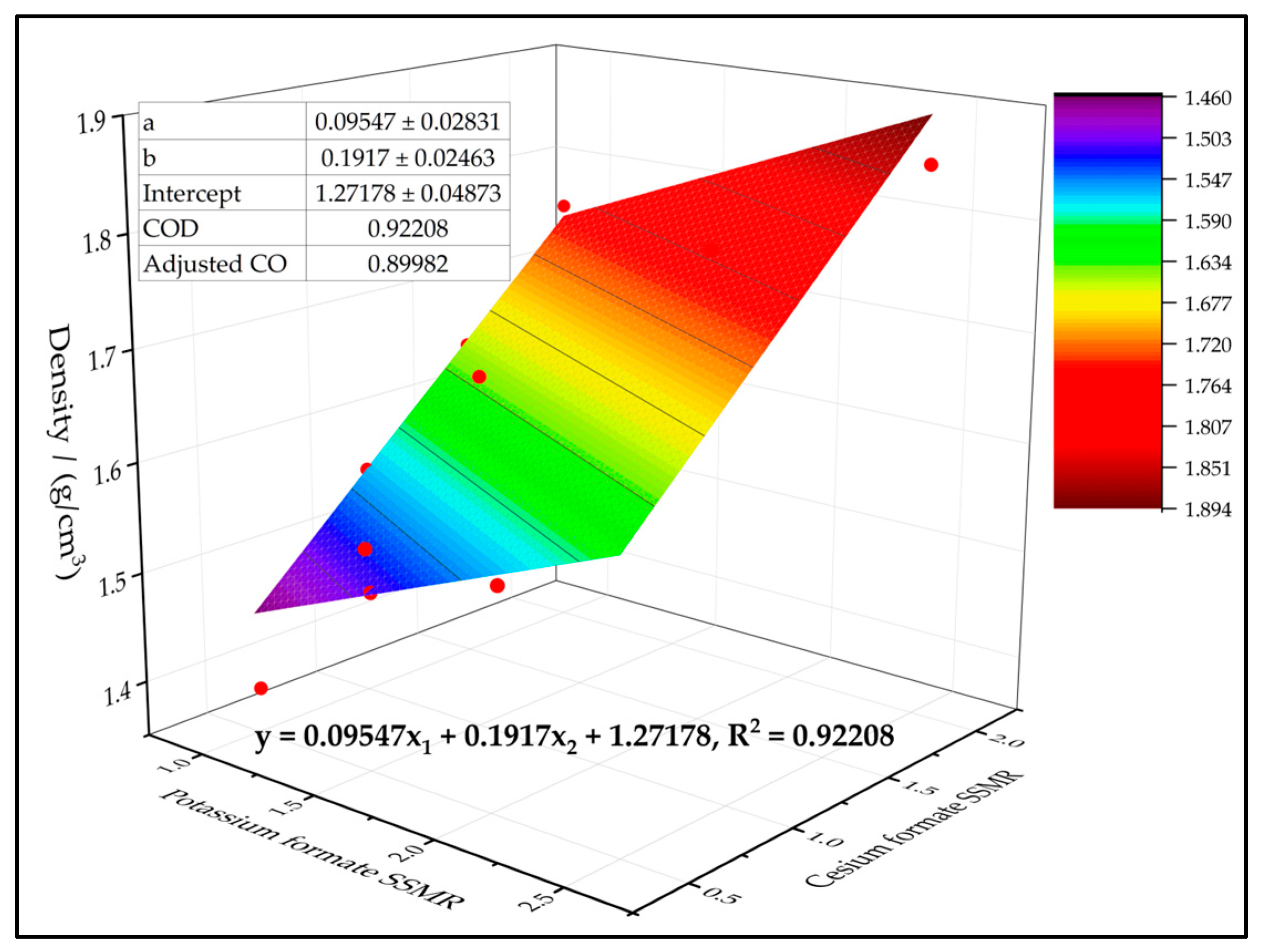
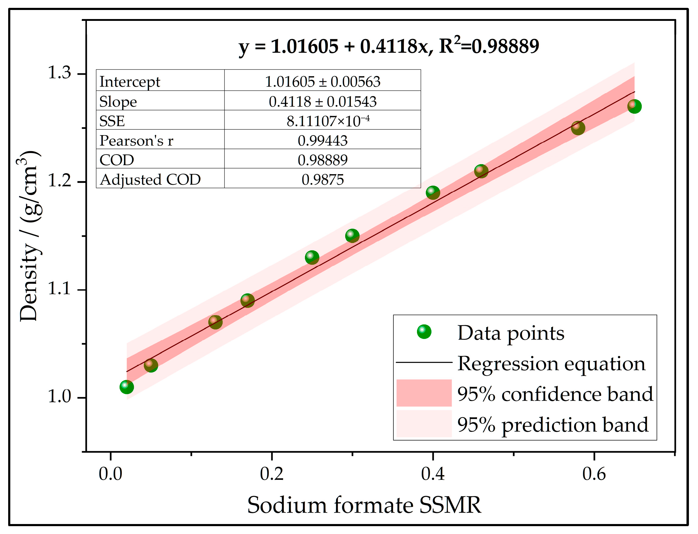
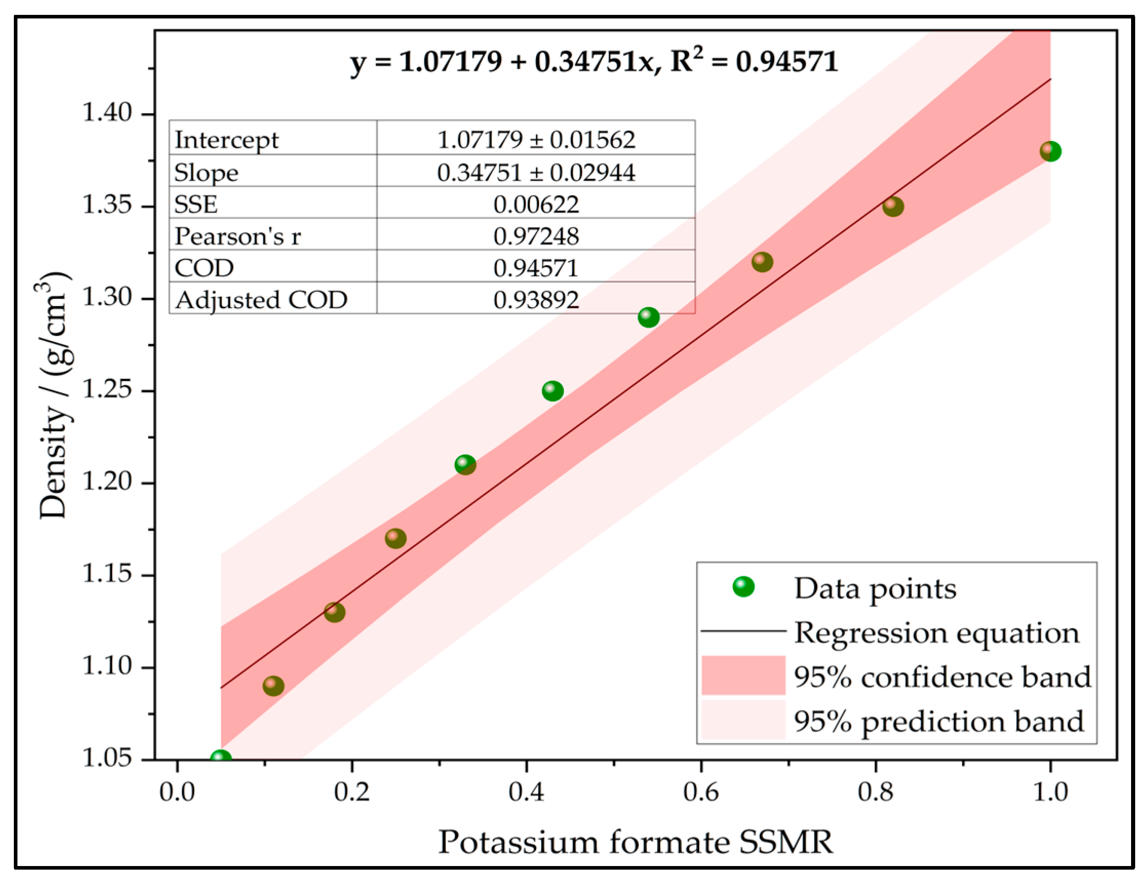
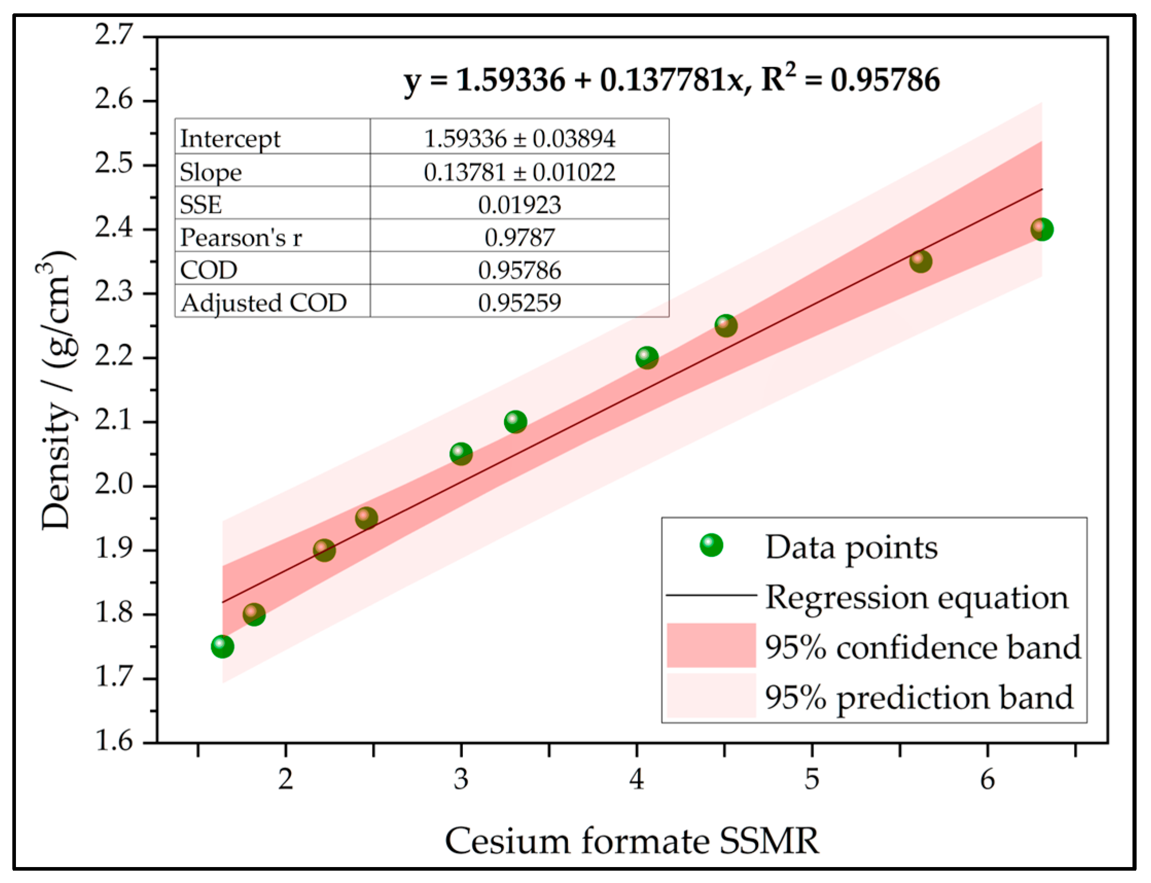
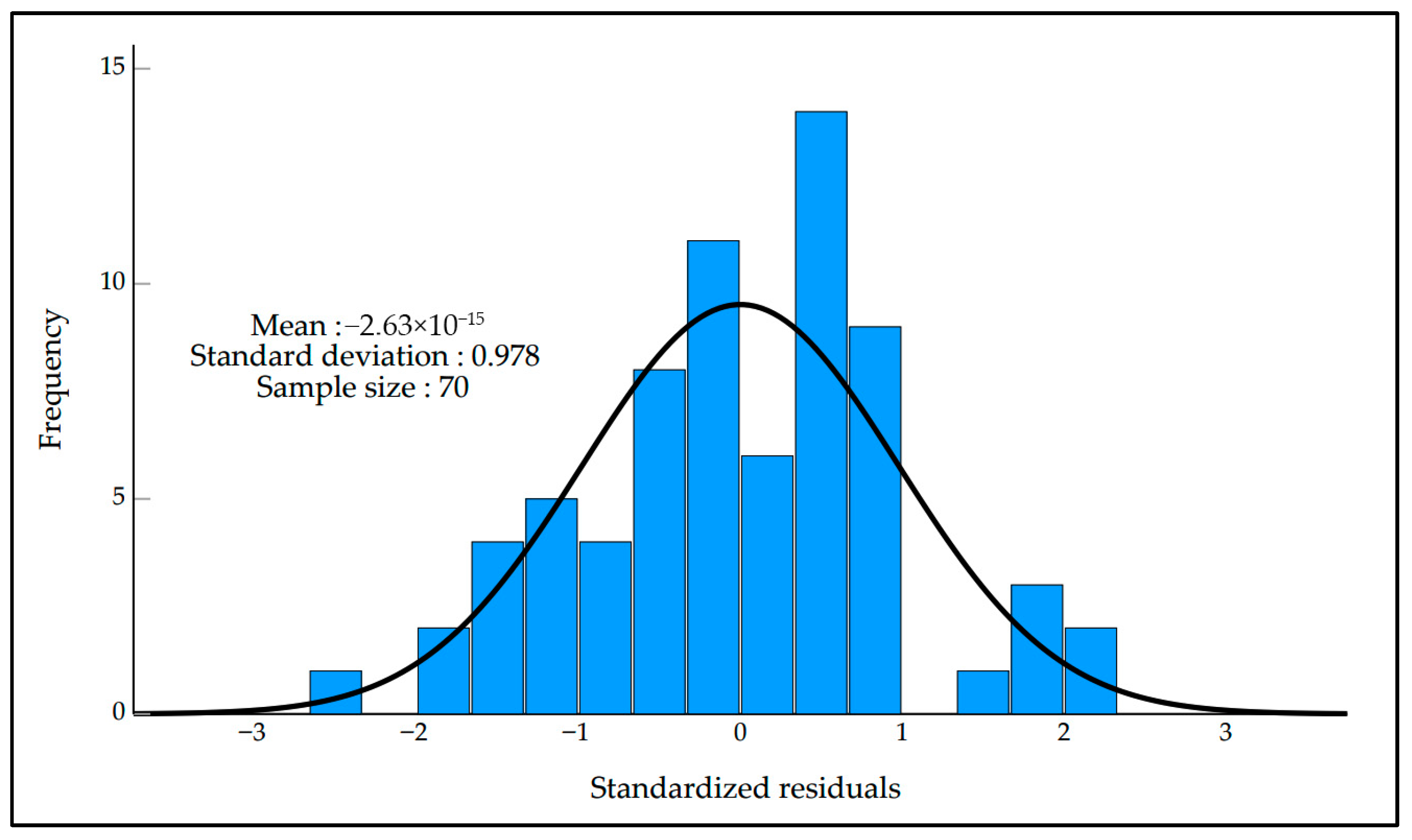
After obtaining the formate solution data through literature survey and laboratory experiments, the solute-to-solvent mass ratio (SSMR) was selected as the independent variable. A multiple linear regression was performed to fit the SSMRs of solutes and the solution density, resulting in multiple linear equations. Six solution systems—comprising single-solute and two-solute solutions—were separately fitted with multiple linear regression, yielding six multiple linear equations. The purpose was to analyze the correlation between solute SSMRs and solution density and to assess the accuracy of the selected data. Finally, for the entire formate solution system, a total of 70 data sets were subjected to multiple linear regression to establish a density model for the formate solution. The equation is expressed in the form of Equation (5).

$$\mathrm{y}=\mathrm{b}+{\mathrm{a}}_1 {\mathrm{x}}_1+{\mathrm{a}}_2 {\mathrm{x}}_2+{\mathrm{a}}_3 {\mathrm{x}}_3+\mathrm{\epsilon }$$

(5)

In Equation (5), y is the density of the formate solution; x_i is the SSMR of the solute, dimensionless; b represents the intercept term; ε denotes the error term, which follows a standard normal distribution.

Although formate brines at high solute-to-solvent mass ratios exhibit pronounced non-ideal electrolyte behavior, including strong ionic interactions and volume contraction, a linear regression model was adopted in this study for engineering-oriented formulation optimization. Within the investigated concentration and density ranges, the experimental and literature data exhibit an approximately monotonic and near-linear relationship between SSMR and solution density, making linear regression an acceptable first-order approximation. Preliminary testing of quadratic and exponential regressions showed only marginal improvements in predictive accuracy while increasing model complexity and reducing interpretability. Physics-based thermodynamic models were not employed because they require extensive interaction parameters and large, high-quality datasets that are currently unavailable for multicomponent formate systems. Given the objective of rapid formulation screening and cost optimization under practical constraints, the linear model provides a transparent and computationally efficient balance between accuracy and engineering applicability.

Based on the formate solution density model, a cost objective function is introduced to realize the reverse calculation of formate solution formulation under density constraints. For a specified solution density, the formulation with the minimum cost is selected through mathematical methods. This problem is similar to a constrained extremum problem, i.e., finding the minimum cost within a certain range. It can be transformed into a linear programming problem for solution. The cost of water is not considered. The mathematical form is shown in Equation (6).

$$\left\{\begin{array}{c}\mathrm{E}=({\mathrm{c}}_1{\mathrm{x}}_1+{\mathrm{c}}_2{\mathrm{x}}_2+{\mathrm{c}}_3{\mathrm{x}}_3) \cdot {\mathrm{m}}_{\mathrm{s}}+{\mathrm{c}}_4{\mathrm{m}}_{\mathrm{s}}\\ \mathrm{y}={\mathrm{a}}_1{\mathrm{x}}_1+{\mathrm{a}}_2{\mathrm{x}}_2+{\mathrm{a}}_3{\mathrm{x}}_3+\mathrm{b}\\ \mathrm{s}.\mathrm{t}.\left(\mathrm{y}\right)\end{array}\right.$$

(6)

In Equation (6), E represents the total cost and serves as the objective function in the linear programming problem, CNY; c_i denotes the unit mass cost of each component, c₄ denotes the unit mass price of industrial water, CNY/kg; y is the solution density, which acts as a constraint in the linear programming model, g/cm³; a_i and b are the coefficients and constant term of the regression equation related to SSMR; m_s is the mass of the solvent, kg. s.t. (y) represents other constraint conditions.

In Equation (6), the parameter m_s is included, where m_s represents the mass of the solvent in the solution. To eliminate the variable solvent mass, m_s needs to be expressed in terms of known parameters, namely the solution density, SSMR values, and the solution volume. Taking a multi-solute solution system as an example, the corresponding expression is given in Equation (7).

$${\mathrm{m}}_{\mathrm{s}}={\displaystyle \frac{1000\mathrm{y}}{1+\sum _{\mathrm{i}}^3{\mathrm{x}}_{\mathrm{i}}}}\cdot \mathrm{V}$$

(7)

In Equation (7), m_s denotes the mass of the solvent, kg; y represents the solution density, g/cm³; V is the solution volume, m³. It should be noted that the solution density is a specified target value rather than a variable and therefore serves as a parameter in the model. In engineering practice, the solution volume is usually predetermined prior to solution preparation; hence, V is also treated as a parameter rather than a variable.

Regarding the additional constraints, the solubility of each solute is finite, which imposes upper limits on the corresponding SSMR values. As a consequence, the achievable solution density is also bounded. Therefore, range constraints on x₁, x₂, x₃, and y must be introduced in the optimization model.

3. Results

3.1. Establishment of the Relationship Between Formate Solution Density and SSMR

For a given solution composed of the same solute(s) and solvent, the solution density can be regarded as a function of SSMR. However, the explicit functional form of this relationship is not predefined. Therefore, multivariate linear regression was employed to fit the experimental data of solution density and SSMR, and a regression equation describing solution density as a function of SSMR was obtained.

3.1.1. Single-Solute Solution Density Model Development

Based on a literature survey, 10 data sets were collected for each single-solute formate solution, including solution density, sodium formate dosage, and water consumption. All data were converted to a basis of 1 m³ solution volume, and the corresponding SSMR values were calculated. These processed data provide the basis for subsequent analysis and modeling. The single-solute solution data for sodium formate [33,34], potassium formate [35], and cesium formate [36,37] are listed in

Table 1. SSMR of single-solute sodium formate, potassium formate, and cesium formate solutions with different densities prepared at 1 m³ (From Literature, Training Dataset).

SSMR of Sodium Formate	Density/(g/cm3)	SSMR of Potassium Formate	Density/(g/cm3)	SSMR of Cesium Formate	Density/(g/cm3)
0.02	1.01	0.05	1.05	1.64	1.75
0.05	1.03	0.11	1.09	1.82	1.8
0.13	1.07	0.18	1.13	2.22	1.9
0.17	1.09	0.25	1.17	2.46	1.95
0.25	1.13	0.33	1.21	3	2.05
0.3	1.15	0.43	1.25	3.31	2.1
0.4	1.19	0.54	1.29	4.06	2.2
0.46	1.21	0.67	1.32	4.51	2.25
0.58	1.25	0.82	1.35	5.62	2.35
0.65	1.27	1	1.38	6.31	2.4

.

As shown in Table 1, for sodium formate solutions, when the SSMR increases from 0.02 to 0.65, the solution density rises from 1.01 g/cm³ to 1.27 g/cm³. For potassium formate solutions, as the SSMR increases from 0.05 to 1.00, the density increases from 1.05 g/cm³ to 1.38 g/cm³. For cesium formate solutions, the density increases from 1.75 g/cm³ to 2.40 g/cm³ as the SSMR increases from 1.64 to 6.31. The corresponding Pearson correlation coefficients are 0.9944, 0.9725, and 0.9787, respectively, all of which are close to 1, indicating a strong correlation. Overall, the densities of the three formate solutions increase monotonically with increasing SSMR; however, their achievable density ranges differ significantly. Sodium formate is suitable for low-density systems, potassium formate for medium-density systems, while cesium formate can meet the requirements of high-density kill and completion fluids.

A simple linear regression was performed on the density and SSMR data of the sodium formate single-solute solutions listed in Table 1 to establish the relationship between solution density and SSMR. The resulting regression equation and the corresponding fitted curve are shown in Figure 3.

As shown in Figure 3, a significant linear relationship exists between the density of the sodium formate solution and SSMR. With increasing SSMR, the solution density increases linearly. The fitted linear equation is y₁ = 0.4118 x₁ + 1.01605. The 95% confidence interval widths of the slope and intercept are 0.01543 and 0.00563, respectively, both of which are relatively small, indicating stable parameter estimation. R² is 0.98889, close to 1, demonstrating a strong linear correlation between the independent and dependent variables with small fitting errors. The confidence band represents the 95% confidence interval around the regression line and is relatively narrow, indicating that the data points are closely distributed around the fitted equation. The prediction band represents the range within which 95% of future observations are expected to fall and is also narrow. Overall, a strong positive linear correlation exists between sodium formate solution density and SSMR.

Based on the density and SSMR data of the potassium formate single-solute solutions listed in Table 1, a simple linear regression analysis was performed to establish the relationship between solution density and SSMR. The resulting regression equation and the corresponding fitted curve are shown in Figure 4.

As shown in Figure 4, a significant linear relationship is observed between the density of potassium formate solutions and SSMR. With increasing SSMR, the solution density increases linearly. The fitted linear equation is expressed as y₂ = 0.34751 x₂ + 1.07179. The 95% confidence intervals of the slope and intercept are both 0.02944, indicating stable parameter estimation. R² is 0.94571, close to unity, suggesting a strong linear correlation between the independent and dependent variables. The confidence band represents the 95% confidence interval around the regression line and is relatively narrow, indicating that the data points are closely distributed around the fitted equation. The prediction band represents the 95% range of predicted values and is comparatively wider, implying potential uncertainty in prediction. However, the predicted values remain within an engineering-acceptable error range of ±10%. Overall, a strong positive linear correlation exists between the density of potassium formate solutions and SSMR.

A simple linear regression was performed on the density and SSMR data of single-solute cesium formate solutions listed in Table 1 The resulting regression equation and corresponding fitted curve are presented in Figure 5.

As shown in Figure 5, a significant linear relationship exists between the density of cesium formate solutions and SSMR. With increasing SSMR, the solution density increases linearly. The fitted linear equation is given as y₃ = 0.137781 x₃ + 1.593336. The 95% confidence interval widths of the slope and intercept are 0.01022 and 0.03894, respectively, both of which are relatively small, indicating stable parameter estimation. R² is 0.95786, close to unity, demonstrating a strong linear correlation between the independent and dependent variables. The confidence band represents the 95% confidence interval around the regression line and is relatively narrow, indicating that the data points are closely distributed around the fitted equation. The prediction band represents the 95% prediction interval and is comparatively wider but remains within the allowable 10% engineering error range. Overall, the density of cesium formate solutions shows a strong positive linear correlation with SSMR.

3.1.2. Binary-Solute Solution Density Model Development

The density, solute dosage, and solvent dosage data of formate-based binary-solute solutions were obtained from laboratory experiments. The experimental data were processed to calculate the SSMR, and the relationship between solution density and SSMR was subsequently established.

(1)

Density Model Development for Sodium Formate–Potassium Formate Binary-Solute Solutions

Based on laboratory experiments, a total of 10 groups of sodium formate–potassium formate binary solutions were prepared. All data were converted to a solution volume of 1 m³, and the corresponding SSMR values were calculated. The processed data are summarized in

Table 2. SSMR of Sodium Formate–Potassium Formate Binary Solutions with Different Densities Prepared at a Volume of 1 m³ (Laboratory Experiments, Training Dataset).

SSMR of Sodium Formate	SSMR of Potassium Formate	SSMR of Cesium Formate	Density/(g/cm3)
0.2	0.5	0	1.28
0.2	1	0	1.39
0.2	2	0	1.52
0.3	0.5	0	1.32
0.3	1	0	1.42
0.3	1.5	0	1.49
0.4	1	0	1.45
0.4	1.5	0	1.5
0.5	1	0	1.46
0.5	1.5	0	1.51

.

As shown in Table 2, when the cesium formate SSMR is zero, the solution density is jointly controlled by the sodium and potassium formate SSMRs. At a sodium formate SSMR of 0.2, increasing the potassium formate SSMR from 0.5 to 2.0 raises the density from 1.28 to 1.52 g/cm³. When the sodium formate SSMR increases to 0.3, the density correspondingly increases to 1.32–1.49 g/cm³ as the potassium formate SSMR varies from 0.5 to 1.5, while further increasing the sodium formate SSMR to 0.4–0.5 leads to a diminished density increment. Pearson correlation coefficients of 0.4654 and 0.9118 indicate that potassium formate SSMR is the primary factor governing density enhancement.

A multiple linear regression analysis was performed on the density data of sodium formate–potassium formate binary-solute solutions in Table 2, and the resulting regression equation and corresponding fitting surface are shown in Figure 6.

As shown in Figure 6, the SSMRs of sodium formate and potassium formate powders exhibit a clear linear relationship with solution density. The fitted multiple linear regression equation is expressed as y₁₂ = 0.25727 x₁ + 0.15045 x₂ + 1.17551. The 95% confidence interval widths of the regression coefficients for the independent variables and the intercept are 0.04981, 0.01218, and 0.02109, respectively, all of which are relatively small, indicating stable parameter estimation. R² is 0.96566, which is close to unity, demonstrating that the model provides an excellent fit to the relationship between solution density and the SSMRs. Therefore, the dependence of solution density on the SSMRs of sodium formate and potassium formate can be well described by this linear regression model.

(2)

Density Model Development for Sodium Formate–Cesium Formate Binary-Solute Solutions

Based on laboratory experiments, ten groups of sodium formate–cesium formate binary-solute solutions were prepared. The solution density, sodium formate dosage, cesium formate dosage, and solvent dosage were recorded. All data were converted to a solution volume of 1 m³, and the corresponding SSMR values were calculated. The detailed data are listed in

Table 3. SSMR of Sodium Formate–Cesium Formate Binary Solutions with Different Densities Prepared at a Volume of 1 m³ (Laboratory Experiments, Training Dataset).

SSMR of Sodium Formate	SSMR of Potassium Formate	SSMR of Cesium Formate	Density/(g/cm3)
0.2	0	0.5	1.25
0.3	0	0.5	1.29
0.5	0	0.5	1.31
0.2	0	1	1.41
0.5	0	1.5	1.63
0.4	0	2	1.65
0.5	0	2	1.69
0.2	0	2	1.71
0.3	0	2	1.73
0.5	0	2.5	1.79

.

As shown in Table 3, when the SSMR of potassium formate is zero, the solution density is mainly governed by the SSMRs of sodium formate and cesium formate. At a cesium formate SSMR of 0.5, increasing the sodium formate SSMR from 0.2 to 0.5 raises the solution density from 1.25 to 1.31 g/cm³. When the cesium formate SSMR increases to 1.0, the solution density reaches 1.41 g/cm³ at a sodium formate SSMR of 0.2. With a further increase in cesium formate SSMR to 2.0, the solution density increases significantly, concentrating in the range of 1.71–1.73 g/cm³ for sodium formate SSMRs between 0.2 and 0.5. When the cesium formate SSMR increases to 2.5 and the sodium formate SSMR is 0.5, the maximum solution density reaches 1.79 g/cm³. The Pearson correlation coefficients are 0.3353 and 0.9841, respectively, indicating that cesium formate plays a dominant role in increasing solution density and is the primary factor for achieving medium- to high-density formate solutions, whereas sodium formate mainly serves as a fine-tuning component. This binary system enables density regulation over a wide range and provides a feasible option for the formulation of high-density kill and completion fluids.

A multiple linear regression was performed on the density, sodium formate SSMR, and cesium formate SSMR data of the sodium formate–cesium formate binary-solute solutions in Table 3, resulting in the relationship between solution density and SSMRs. The regression equation and corresponding plot are shown in Figure 7.

As shown in Figure 7, As the SSMRs of sodium formate and cesium formate increase, a linear relationship is observed between the SSMRs of sodium formate and cesium formate powders and the solution density. The fitted linear equation is y₁₃ = 0.06365 x₁ + 0.26415 x₃ + 1.14007. The 95% confidence intervals of the regression coefficients and intercept are 0.10541, 0.01867, and 0.04144, respectively, all of which are relatively small, indicating that the model parameters are stably estimated. The R2 is 0.97000 and is close to 1, indicating that the model fits well the relationship between solution density and SSMR. Therefore, the relationship between the density of sodium formate–cesium formate binary solutions and their SSMRs can be described by this linear fitting equation.

(3)

Density Model Development for Potassium Formate–Cesium Formate Binary-Solute Solutions

Laboratory experiments were conducted to prepare 10 potassium formate–cesium formate binary-solute solutions. The solution density, solute amounts, and solvent quantity were recorded, converted to a 1 m³ solution basis, and used to calculate SSMRs. The detailed data are listed in

Table 4. SSMRs of Potassium Formate–Cesium Formate Binary-Solute Solutions with Different Densities Prepared at a Volume of 1 m³ (Laboratory Experiments, Training Dataset).

SSMR of Sodium Formate	SSMR of Potassium Formate	SSMR of Cesium Formate	Density/(g/cm3)
0	1	0.51	1.39
0	1.5	1.01	1.67
0	2.5	2	1.85
0	2.03	1.5	1.78
0	1	1.01	1.56
0	1	1.5	1.65
0	1	2	1.76
0	1.5	0.51	1.51
0	2.03	0.5	1.55
0	1.5	0.49	1.55

.

As shown in Table 4, under the condition of SSMR of sodium formate being 0, the solution density is jointly determined by potassium formate and cesium formate. When the SSMR of potassium formate is 1, increasing the SSMR of cesium formate from 0.51 to 2.00 gradually raises the solution density from 1.39 g/cm³ to 1.76 g/cm³. When the SSMR of potassium formate is increased to 1.5, the solution density is approximately 1.51 g/cm³ at a cesium formate SSMR of around 0.5, and it rises to 1.67 g/cm³ as cesium formate increases to about 1.5. Further increasing the SSMR of potassium formate to 2.03–2.5, together with a cesium formate SSMR of 1.5–2.0, allows the solution density to reach 1.78–1.85 g/cm³. In the absence of sodium formate, the synergistic density-increasing effect of potassium and cesium formates is significant, with Pearson correlation coefficients of 0.4975 and 0.8919, respectively, indicating that cesium formate contributes more prominently to density enhancement, while potassium formate primarily serves to expand the density adjustment range. This system can achieve a medium-to-high density range of 1.39–1.85 g/cm³, suitable for the formulation of high-density kill and completion fluids.

A multivariate linear regression was performed on the solution density, SSMR of potassium formate, and SSMR of cesium formate in Table 4, resulting in the relationship between solution density and SSMRs. The regression equation and corresponding plot are shown in Figure 8.

As shown in Figure 8, the SSMRs of potassium formate and cesium formate powders exhibit a linear relationship with the solution density, forming a plane in three-dimensional space. The fitted linear equation is y₂₃ = 0.09547 x₂ + 0.1917 x₃ + 1.27178. The 95% confidence intervals of the coefficients and intercept are 0.02831, 0.02463, and 0.04873, respectively, all relatively small, indicating stable parameter estimates. The coefficient of determination R² is 0.92208. The R² value close to 1 indicates that the model fits the relationship between solution density and SSMRs well. Therefore, the solution density of the potassium and cesium formate mixture can be described using this linear regression equation.

In summary, density models were established for single-solute and multi-solute formate solutions. The R² values of the six models are 0.98889, 0.94571, 0.95786, 0.96566, 0.97000, and 0.92208, all close to 1, indicating excellent model fitting and reasonable selection of training data. The above data can be used for constructing density models of multi-solute formate solutions.

3.1.3. Multi-Solute Solution Density Model Development

Laboratory experiments were conducted to prepare solutions containing three solutes: sodium formate, potassium formate, and cesium formate. Within the solubility limits of formic acid, potassium formate, and cesium formate, and within the density range of undersaturated three-solute solutions, ten sets of sodium–potassium–cesium formate solutions were prepared. The undersaturated solution density, amounts of sodium formate, potassium formate, cesium formate, and water were recorded, and all data were converted to a 1 m³ solution basis. The SSMRs were then calculated. The detailed data are presented in

Table 5. SSMRs of Sodium Formate–Potassium Formate–Cesium Formate Ternary-Solute Solutions with Different Densities Prepared at a Volume of 1 m³ (Laboratory Experiments, Training Dataset).

SSMR of Sodium Formate	SSMR of Potassium Formate	SSMR of Cesium Formate	Density/(g/cm3)
0.2	1	0.5	1.52
0.2	1.5	1	1.68
0.3	1.5	1	1.68
0.4	1.51	1	1.68
0.4	2	1	1.7
0.4	2.5	1	1.72
0.2	2.5	2	1.85
0.3	2.5	2	1.85
0.41	2.5	2	1.85
0.2	1.5	0.49	1.58

.

As shown in Table 5, under the simultaneous presence of sodium formate, potassium formate, and cesium formate, the solution density increases with the overall rise in the SSMRs of the three formates. When the SSMR of cesium formate is 1, with sodium formate varying from 0.2 to 0.4 and potassium formate from 1.5 to 2.5, the solution density is mainly concentrated between 1.68 and 1.72 g/cm³, showing a small variation. When the SSMR of cesium formate increases to 2, under the conditions of potassium formate at 2.5 and sodium formate between 0.2 and 0.41, the solution density stably reaches 1.85 g/cm³. In contrast, at a lower cesium formate SSMR (around 0.5), even with simultaneous increases in sodium and potassium formates, the solution density only reaches approximately 1.52–1.58 g/cm³. The Pearson correlation coefficients are 0.3441, 0.8954, and 0.9694, respectively. Therefore, in the multi-solute system, cesium formate remains the key factor controlling the solution density level, potassium formate mainly serves to fine-tune the density adjustment range, and sodium formate has a relatively small effect on density. The combination of the three allows the preparation of stable medium-to-high density formate solutions over a relatively wide range of dosages.

Multivariate linear regression was performed on the solution density, SSMRs of sodium formate, potassium formate, and cesium formate in Table 1, Table 2, Table 3, Table 4 and Table 5, resulting in the relationship between solution density and SSMRs. The regression equation is shown in Equation (8).

y = 0.0898 x₁ + 0.1217 x₂ + 0.2271 x₃ + 1.1982

(8)

In Equation (8), y is the solution density, g/cm³; x₁ is the SSMR of sodium formate; x₂ is the SSMR of potassium formate; and x₃ is the SSMR of cesium formate.

In multiple linear regression models, the random error terms are typically assumed to be independently and identically distributed and to follow a normal distribution with a mean of zero and a variance of σ². The residual analysis is shown in the figure below.

Figure 9. Standardized Residual Histogram.

Figure 9. Standardized Residual Histogram.

As shown in Figure 9, the standardized regression residuals exhibit an overall unimodal distribution with a mean close to zero, and the majority of residuals fall within the range of ±2. This indicates that no pronounced systematic bias exists at the overall scale and that the residual level remains within an acceptable range. Although the residual distribution shows some deviation from the ideal normal distribution, such deviation does not present significant abnormality given the relatively limited sample size (n = 70) and the tolerance typically allowed in engineering applications.

Figure 10. Scatter plot of standardized residuals versus standardized predicted values.

Figure 10. Scatter plot of standardized residuals versus standardized predicted values.

As shown in Figure 10, the scatter distribution of residuals versus predicted values indicates that the residuals are not completely random, showing certain structured patterns within specific prediction intervals. This behavior is commonly observed in empirical modeling of non-ideal systems such as high-concentration electrolyte solutions, reflecting nonlinear effects and complex interactions that are not fully captured by simple linear regression models. In addition, the residuals do not increase systematically with predicted values, nor do they exhibit pronounced extreme outliers, indicating that the model maintains stable predictive behavior within the investigated range. Overall, the standardized regression residuals exhibit a unimodal distribution with a mean close to zero, and most residuals fall within the range of ±2, indicating that the overall error level of the model is well controlled and that no significant systematic bias exists. The residuals do not increase systematically with predicted values, nor are obvious outliers observed, suggesting that the model shows good engineering applicability within the studied variable range.

Regression analysis of the model was conducted, and the related statistics are summarized in

Table 6. Regression Statistics of the Density Model for Multi-Solute Formate Solutions.

Statistical Magnitude	Multiple R	R Square	Adjusted R Square
value	0.95719109	0.91621479	0.91240637

.

As shown in Table 6, the core fitting indicators of this multivariate linear regression model perform excellently. Constructed based on a sufficient sample size of 70, the model has adequate data support. The multiple correlation coefficient (Multiple R) is 0.9572, indicating a very strong positive correlation between the dependent variable and the three independent variables. The coefficient of determination (R²) is 0.9162, close to 1, demonstrating excellent model fit. The adjusted R², which accounts for the number of independent variables, is 0.9124, indicating stable fitting. The standard error of the model is only 0.0964, reflecting a low error level. Overall, the goodness-of-fit is very high, providing a solid foundation for subsequent analysis and prediction.

Analysis of variance (ANOVA) was conducted for the model, and the related statistical results are presented in

Table 7. ANOVA Indicators for the Density Model of Multi-Solute Formate Solutions.

	Df	Sum of Squares	Mean Square	F	Significance F
Regression	3	6.71177202	2.23725734	240.576177	1.8311 × 10−35
Error	66	0.61377226	0.00929958
Total Sum of Squares	69	7.32554429

.

As shown in Table 7, the model is highly significant overall. In terms of sums of squares and mean squares, SSR = 6.7118 is much larger than SSE = 0.6138, and MSR = 2.2373 is significantly higher than MSE = 0.0093. The F statistic of the regression model reaches 240.58, with a p-value of 1.83 × 10⁻³⁵, far below the 0.05 significance level. This indicates that the three independent variables jointly explain the variation in the dependent variable very effectively, and the model is not a random fit. Its overall accuracy and statistical significance are well validated.

The significance of the independent variables in the model was analyzed, and the related statistical indicators are presented in

Table 8. Significance Analysis of Independent Variables for the Density Model of Multi-Solute Formate Solutions.

	Coefficients	Standard Error	t Stat	p-Value	Lower 95%	Upper 95%
Intercept	1.19817826	0.02251609	53.2143078	6.198 × 10−56	1.15322344	1.24313309
X1 Variable	0.08979743	0.06135834	1.46349189	0.14807936	−0.0327084	0.2123033
X2 Variable	0.12172674	0.0142201	8.56018955	2.6384 × 10−12	0.0933354	0.15011809
X3 Variable	0.22708828	0.00875786	25.9296456	2.5269 × 10−36	0.20960265	0.24457392
Intercept	1.19817826	0.02251609	53.2143078	6.198 × 10−56	1.15322344	1.24313309

.

As shown in Table 8, the significance test of independent variables (t-test) aims to determine whether a single independent variable has a statistically significant effect on the dependent variable. The core is to judge whether the coefficients of the independent variables are significantly different from zero using the t statistic, p-value, and 95% confidence interval. Analysis of the model shows that the intercept coefficient is 1.1982 (standard error 0.0225), with a t statistic of 53.21, a 95% confidence interval of [1.1532, 1.2431], and a p-value of 6.20 × 10⁻⁵⁶, indicating that the baseline value of the dependent variable is reliable when all independent variables are zero. The coefficient of X₁ is 0.0898 (standard error 0.0614), with a t statistic of 1.46, confidence interval [−0.0327, 0.2123], and p-value 0.1481, which is relatively large. The coefficient of X₂ is 0.1217 (standard error 0.0142), with a t statistic of 8.56, confidence interval [0.0933, 0.1501], and p-value 2.64 × 10⁻¹², extremely small. The coefficient of X₃ is 0.2271 (standard error 0.0088), with a t statistic of 25.93, confidence interval [0.2096, 0.2446], and p-value 2.53 × 10⁻³⁶, extremely small.

The regression coefficient of sodium formate (corresponding to the X₁ variable) is positive (0.0898), indicating a potentially weak positive effect on solution density; however, its p-value is 0.148 (>0.05), suggesting that the effect is not statistically significant. Considering the characteristics of the model and the dataset, this result may be attributed to three factors. First, solution density exhibits relatively low sensitivity to sodium formate concentration. Compared with variables X₂ and X₃, which show extremely high statistical significance (p-values of 2.6384 × 10⁻¹² and 2.5269 × 10⁻³⁶, respectively), the explanatory power of sodium formate is considerably weaker. Second, potential multicollinearity may exist, as sodium formate could be correlated with X₂ and X₃, leading to inflated standard errors. Third, the concentration range of sodium formate in the dataset is relatively narrow and does not cover critical intervals, limiting the model’s ability to capture its intrinsic relationship with density. Overall, the non-significant effect of sodium formate is more likely the combined result of multicollinearity and limited data range rather than the absence of a physical influence.

In summary, the model baseline is reasonably set. The SSMR of sodium formate has a weak effect on density, while the SSMRs of potassium and cesium formates are key positive factors affecting the dependent variable, with cesium formate having the most pronounced impact.

3.2. Reverse Calculation of Minimum-Cost Formate Solution Composition Under Density Constraint

The SSMRs of saturated single-solute solutions of sodium formate, potassium formate, and cesium formate are 0.812, 3.37, and 4.5, respectively. The unit prices per kilogram of sodium formate, potassium formate, and cesium formate are 4 CNY/kg, 8 CNY/kg, and 100 CNY/kg, respectively. The water cost per kilogram is approximately 0.004 CNY/kg. The unit prices of formates are not fixed and may fluctuate with the market. Taking the above unit prices and a solution volume of 1 m³ as an example, this study performs a reverse calculation to determine the minimum-cost solution composition under a density constraint.

3.2.1. Reverse Calculation of Minimum-Cost Single-Solute Solution Composition Under Density Constraint

For single-solute solutions, cost optimization under a density constraint does not exist. Under constant environmental conditions, if the solution volume and density are fixed, the total mass of the solution is also determined. Considering that the solution density is a function of the SSMR, different solute-to-solvent mass ratios will result in changes in density. Therefore, specifying the density uniquely determines the SSMR. It can be further inferred that the masses of both solute and solvent are also fixed. This is corroborated by the fitted density equation, which is a monotonic function; its inverse function exists and is also monotonic, so a fixed density corresponds to a unique SSMR. Consequently, when both the volume and density are fixed, the masses of solute and solvent are determined, and thus the cost is fixed—there is no variation in cost to optimize.

3.2.2. Reverse Calculation of Minimum-Cost Multi-Solute Solution Composition Under Density Constraint

Multi-solute solutions differ from single-solute solutions. A multi-solute solution consists of multiple solutes, each with its own SSMR. For the same density, there are multiple possible combinations of solute SSMRs, each corresponding to a different cost. Therefore, for multi-solute solutions, the same density can correspond to solutions with varying costs. Moreover, multi-solute solutions include single-solute solutions as a special case. If it is not predetermined whether to prepare a single-solute or multi-solute solution and only cost is considered, the density model for multi-solute solutions can also yield the composition of single-solute solutions.

The cost function serves as the objective function and is combined with Equation (6) for parameter elimination. The multi-solute formate solution density equation (Equation (8)) serves as a constraint. In addition, the solubility limits of the formates and the solution density range are considered. A reverse calculation model for the minimum-cost composition of multi-solute solutions under a density constraint is thus established, as expressed mathematically in Equation (9).

$$\left\{\begin{array}{c}\mathrm{E}=(4{\mathrm{x}}_1+8{\mathrm{x}}_2+100{\mathrm{x}}_3)\cdot {\mathrm{m}}_{\mathrm{s}}+0.004{\mathrm{m}}_{\mathrm{s}}\\ {\mathrm{m}}_{\mathrm{s}}={\displaystyle \frac{1000\mathrm{y}}{1+{ \mathrm{x}}_1+{ \mathrm{x}}_2+{ \mathrm{x}}_3}}\\ \mathrm{y}=0.0898{ \mathrm{x}}_1+0.1217{ \mathrm{x}}_2+0.2271{ \mathrm{x}}_3+1.1982\\ 0 \le { \mathrm{x}}_1 \le 0.812\\ 0 \le { \mathrm{x}}_2 \le 3.37\\ 0 \le { \mathrm{x}}_3 \le 4.5\\ 1.20 \le \mathrm{y} \le 2.35\end{array}\right.$$

(9)

In Equation (9), E is the cost objective function, CNY; y is the solution density, g/cm³; m_s is the mass of the solvent, kg; x_i is the SSMR of the solute, dimensionless.

Based on Equation (9), five density points within the solubility range were selected to calculate the minimum-cost solution compositions. The solution densities, minimum costs, and solute SSMRs are summarized in

Table 9. Reverse Calculation Data of Minimum-Cost Multi-Solute Solution Compositions under Density Constraint.

Density y/(g/cm3)	Minimum Cost Value E/CNY	SSMR of Sodium Formate x1	SSMR of Potassium Formate x2	SSMR of Cesium Formate x3
1.25	1832.26	0.577	0.000	0.000
1.45	6631.60	0.812	1.470	0.000
1.7	12,409.17	0.812	3.370	0.082
1.95	45,499.07	0.812	3.370	1.183
2.2	76,203.18	0.812	3.370	2.284

.

As shown in Table 9, at a density of 1.25 g/cm³, the minimum cost is 1829.54 CNY, with SSMRs of sodium formate, potassium formate, and cesium formate of 0.577, 0, and 0, respectively. At a density of 1.45 g/cm³, the minimum cost is 6630.08 CNY, corresponding to SSMRs of 0.812, 1.470, and 0. At a density of 1.70 g/cm³, the minimum cost is 12,410.51 CNY, with SSMRs of 0.812, 3.370, and 0.082. When the density increases to 1.95 g/cm³, the minimum cost rises to 45,499.91 CNY, and the corresponding SSMRs are 0.812, 3.370, and 1.183. At a density of 2.20 g/cm³, the minimum cost reaches 76,203 CNY, with SSMRs of 0.812, 3.370, and 2.284. Overall, under a density constraint, the model can determine the minimum cost and inversely calculate the corresponding solute SSMRs, demonstrating its applicability.

4. Discussion

Equation (8) represents the mathematical algorithm underlying the model. Overall, the model computation consists of two main parts. The first part is the establishment of the relationship between the density of multi-solute solutions and the solute SSMRs. The second part is the formulation of a cost objective function to achieve the reverse calculation of the minimum-cost composition of multi-solute solutions at a specified density.

The second part consists of purely algebraic calculations and introduces no error; all errors originate from the first part. These errors mainly arise from experimental operations and sample purity, as well as from the theoretical error of the multivariate linear regression model.

A total of 21 validation experimental points were designed. During the experiments, all formate solutions were prepared in the laboratory according to the predefined schemes, and their densities were measured experimentally as the true density values for each validation point. Meanwhile, the solute SSMRs were substituted into the fitted equations, and the densities calculated by the respective models were regarded as the observed densities. Differences exist between the true densities and the model-predicted densities. When the error falls within the range [0, 0.5], the model is considered excellent; when the error lies in the range (0.5, 1], the model is considered good; and when the error exceeds 1, the model is considered fair. The detailed error data are presented in

Table 10. Error Analysis of Minimum-Cost Composition Back-Calculation for Multisolute Solutions under Density Constraint (Laboratory Experiments, Test Dataset).

SSMR of Sodium Formate	SSMR of Potassium Formate	SSMR of Cesium Formate	Measured Density	Predicted Density	Error/(g/cm3)
0.1	0	0	1.15	1.21	0.05
0.2	0	0	1.2	1.22	0.01
0.35	0	0	1.27	1.23	−0.03
0	0.3	0	1.24	1.23	−0.00
0	0.5	0	1.31	1.26	−0.04
0	1	0	1.45	1.32	−0.09
0	0	0.5	1.36	1.31	−0.04
0	0	0.7	1.5	1.36	−0.10
0	0	1	1.64	1.43	−0.13
0.2	1.5	0	1.57	1.40	−0.11
0.3	2	0	1.65	1.47	−0.11
0.1	0.5	0	1.35	1.27	−0.06
0.2	0	0.7	1.35	1.38	0.02
0.3	0	0.7	1.36	1.38	0.02
0.4	0	0.5	1.33	1.35	0.01
0	1.5	0.7	1.53	1.54	0.01
0	2.51	0.7	1.64	1.66	0.01
0	2	0.6	1.67	1.58	−0.06
0.4	1	0.5	1.58	1.47	−0.07
0.4	2	0.5	1.61	1.59	−0.01
0.3	1	0.7	1.5	1.51	0.00

.

As shown in Table 10, there are discrepancies between the predicted densities obtained from the density prediction model and the measured densities. Calculations indicate that the mean squared error (MSE) of the model predictions is 0.00885, the root mean squared error (RMSE) is 0.094 g/cm³, and the mean absolute error (MAE) is 0.07 g/cm³. By normalizing these errors with respect to the average measured density of 1.44 g/cm³, the relative mean absolute error (rMAE) and the relative root mean squared error (rRMSE) are approximately 4.9% and 6.5%, respectively. Therefore, the model exhibits good predictive stability for most samples. However, the RMSE is higher than the MAE, indicating the presence of relatively large prediction deviations in a small number of samples. Overall, the model satisfies the requirements of engineering accuracy.

From an engineering perspective, fluid density requirements are defined within an allowable density window rather than as a single target value. In practical operations, this window is typically wider than the average prediction deviation observed in this study. The mean absolute error of 0.07 g/cm³ therefore represents a relatively small fraction of the operational density window and can be readily accommodated through routine on-site adjustment. Consequently, the achieved prediction accuracy is considered reasonable and sufficient for formulation guidance and cost optimization within engineering applications.

An analysis of the sources of prediction errors in cesium formate solution systems. For high-density cesium formate brines, nonlinear behavior becomes more pronounced due to strong electrolyte non-ideality. At elevated concentrations, high ionic strength and strong short-range interactions between Cs⁺ and formate ions lead to significant deviations from ideal solution behavior. In addition, pronounced volume contraction and changes in hydration structure reduce the linear proportionality between solute addition and density increase. These effects are further amplified near solubility limits, where small composition variations can induce disproportionate density changes. Consequently, density–composition relationships in high-density cesium formate systems inherently exhibit nonlinear characteristics.

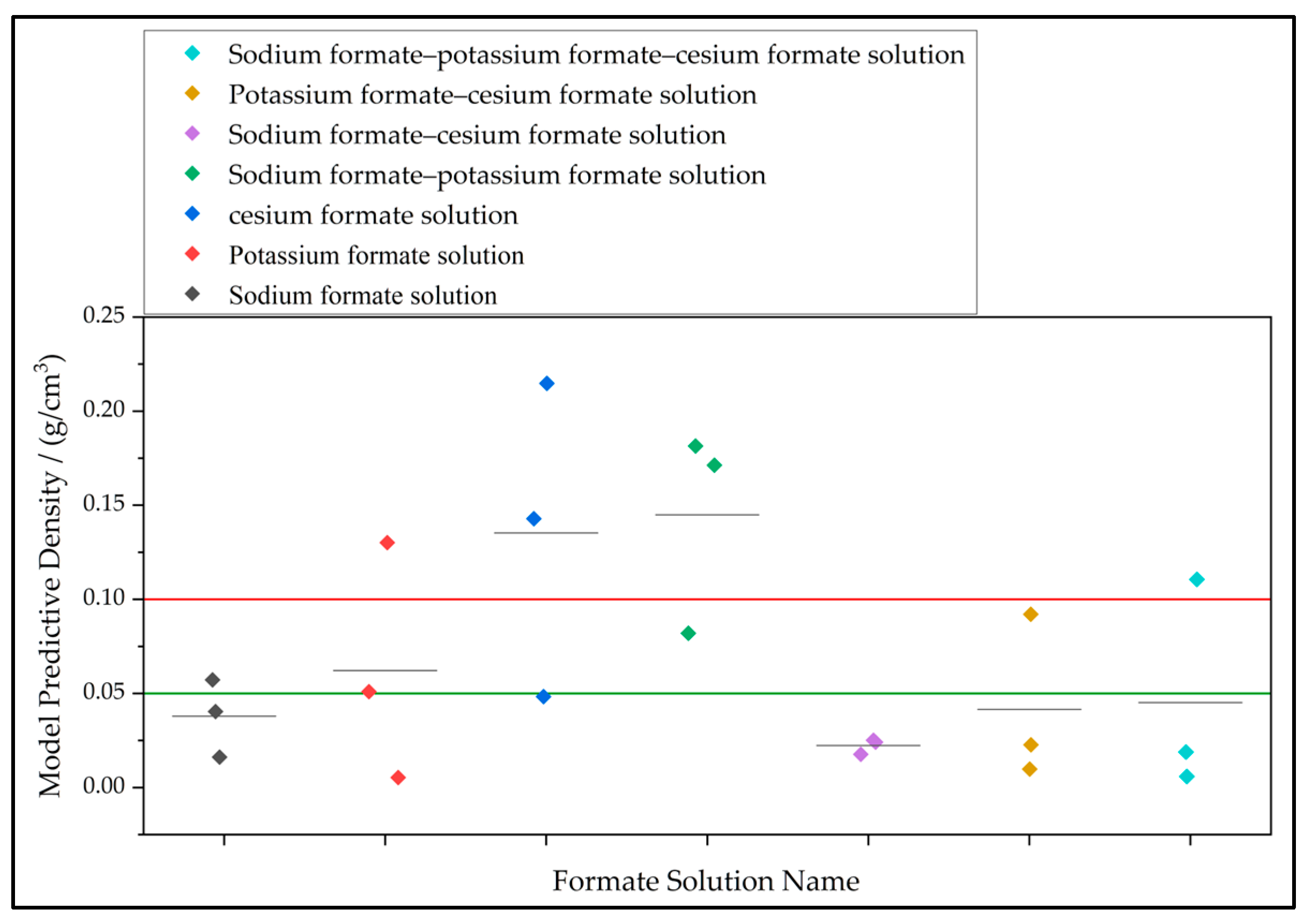
To provide a more intuitive comparison between the model prediction errors and the error evaluation criteria, the prediction errors were plotted as a grouped scatter diagram, as shown in Figure 11.

As shown in Figure 11, when the model is applied to sodium formate solutions, the mean density error is 0.038 g/cm³; for potassium formate solutions, the mean density error is 0.062 g/cm³; for cesium formate solutions, the mean density error is 0.135 g/cm³.

For sodium formate–potassium formate solutions, the mean density error is 0.145 g/cm³; for sodium formate–cesium formate solutions, it is 0.022 g/cm³; for potassium formate–cesium formate solutions, it is 0.042 g/cm³; and for sodium formate–potassium formate–cesium formate solutions, the mean density error is 0.045 g/cm³. Based on the mean error values, the model performance is classified as excellent for sodium formate and cesium formate single-solute solutions, good for potassium formate single-solute solutions, and excellent for sodium formate–potassium formate–cesium formate multisolute solutions.

5. Conclusions

This study focuses on the minimum-cost formulation problem of formate solutions under density constraints. Model development and experimental validation were conducted, and the expected objectives were basically achieved. Based on the literature investigation and laboratory experiments, 10 experimental groups were designed, yielding a total of 70 data sets. On the basis of these data, formate solution density models were established through regression fitting. By introducing a cost objective function and combining a data-driven optimization method, the minimum-cost formulation under density constraints was back-calculated. Accuracy evaluation experiments were further designed. The main conclusions and recommendations are as follows.

(1)

Theoretical aspect

Based on literature and laboratory data, the solute-to-solvent mass ratio (SSMR) was proposed as the independent variable for model fitting, and it was demonstrated that the density of a given solution depends only on the SSMR. Although strict theoretical derivation is not mandatory in engineering practice, it is still recommended that future studies further investigate particle interaction mechanisms to provide a deeper theoretical explanation of the relationship between solution density and SSMR.

(2)

Model development

Density models for sodium formate, potassium formate, and cesium formate single-solute solutions, as well as multisolute formate solutions, were established. The fitted equation is y = 0.0898 x₁ + 0.1217 x₂ + 0.2271 x₃ + 1.1982, with an R² value of 0.91241, which is close to unity. The model can effectively describe the density variation in formate solutions. Only linear models were considered in this study; although the accuracy is excellent, considering the strong ionic interactions and volume contraction effects in high-concentration formate brines, it is necessary to supplement the training dataset and introduce nonlinear models, such as quadratic or exponential regressions, to further improve prediction accuracy.

(3)

Model accuracy

When applied to seven types of formate solutions, the mean density prediction errors are 0.038 g/cm³, 0.062 g/cm³, 0.135 g/cm³, 0.145 g/cm³, 0.022 g/cm³, 0.042 g/cm³, and 0.045 g/cm³, respectively. The root mean square error (RMSE) is 0.094 g/cm³, and the mean absolute error (MAE) is 0.07 g/cm³. The relative MAE (rMAE) and relative RMSE (rRMSE) are approximately 4.9% and 6.5%, respectively. Although relatively large deviations occur for a small number of samples, the overall results indicate that the model meets engineering accuracy requirements. The larger errors are mainly attributed to limited training data or the local data concentration; therefore, expanding the training dataset is recommended.

Overall, this study establishes a data-driven framework for minimum-cost formulation design of formate solutions under density constraints by introducing the SSMR as the key independent variable and integrating regression modeling with cost optimization. The proposed approach demonstrates satisfactory predictive accuracy and practical applicability at the engineering level. Nevertheless, limitations related to the dataset scale, linear model assumptions, and empirical characterization indicate that further improvements can be achieved by expanding experimental data, incorporating nonlinear modeling techniques, and strengthening physicochemical interpretation. These efforts are expected to enhance model robustness and support more comprehensive formulation optimization in future applications.