Rig State Classification Using Class-Specific Attribute-Weighted Pseudo-Dynamic Bayes for Invisible Lost Time Evaluation

Abstract

Oil and gas drilling is a capital-intensive industry where minimizing costs is paramount. Invisible Lost Time (ILT) during drilling often causes delays and escalates expenses. Accurate rig state classification is critical for quantifying ILT and improving drilling efficiency. In this study, we introduce a novel rig state classification model based on the Class-Specific Attribute Weighted Pseudo-Dynamic Bayes (CAWPDB) algorithm. Unlike existing machine learning methods, which often underutilize domain knowledge, our approach seamlessly integrates drilling expertise by constructing a pseudo-dynamic Bayesian model informed by an expert-derived state transition matrix. To overcome the limitations of the attribute conditional-independence assumption and boost classification performance, we incorporate a class-specific attribute-weighting mechanism. Experimental results from two wells demonstrate that the model achieves a 99.985% accuracy in identifying rig states from surface sensor data, with outstanding performance even for low-frequency rig states. This research enhances ILT visualization and provides valuable insights for optimizing drilling operations and reducing costs.

1. Introduction

Drilling engineering represents a fundamental pillar of hydrocarbon resource development yet remains one of the most technically challenging, capital-intensive, and risk-laden disciplines within the energy sector. Optimizing drilling efficiency while minimizing operational costs has therefore become a critical priority for ensuring project economic viability. Modern drilling operations must maintain rigorous compliance with time and budget constraints while simultaneously addressing three primary objectives: maximizing rate of penetration (ROP), preserving wellbore integrity, and strategically accelerating operational timelines. However, field operations frequently encounter numerous downhole complications and drilling anomalies that disrupt workflow continuity, prolong operational durations, and increase project expenditures. This accumulated operational downtime is formally categorized as Non-Productive Time (NPT) [1].

From a comprehensive operational perspective, NPT encompasses all drilling interruptions and can be subdivided into two distinct categories: Visible Lost Time (VLT) and Invisible Lost Time (ILT). VLT specifically measures observable downtime resulting from diagnosing and resolving downhole problems or equipment failures. Conversely, ILT represents hidden inefficiencies embedded within routine drilling operations—such as tripping procedures, pipe connections, and rotary operations—stemming from suboptimal practices, equipment performance constraints, and variations in crew proficiency. Significantly, even minor cycle time deviations of mere seconds per operation can accumulate across multiple drilling phases, ultimately resulting in considerable project delays and cost overruns [2]. While manual VLT tracking has proven operationally viable, as demonstrated by De Oliveira et al. [3], the complexity and real-time nature of modern drilling data streams make manual ILT quantification both impractical and error-prone. This limitation highlights the critical need for automated monitoring systems equipped with advanced analytical capabilities to achieve accurate ILT measurement and enable operational optimization.

Accurate quantification of Invisible Lost Time (ILT) in drilling operations fundamentally relies on precise rig state classification—a methodological requirement well-established in the literature. However, the labor-intensive nature of manual classification makes it impractical for field deployment. Recent advances in machine learning have successfully addressed complex engineering challenges in petroleum systems, driving extensive research into automated rig state identification and ILT computation. Sun et al. [4] pioneered a Support Vector Machine (SVM) framework that achieved detailed classification across six operational states. Incorporating temporal aspects of drilling dynamics, Yin et al. [5,6] developed a Long Short-Term Memory (LSTM)-based system optimized for deepwater drilling mode recognition. Similarly, Tran et al. [7] demonstrated improved diagnostic capabilities using a hybrid CNN-LSTM architecture for real-time drill bit failure detection. Ben et al. [8] systematically evaluated Random Forest, CNN, and hybrid CNN/RNN models for processing high-frequency drilling signals, establishing comprehensive KPI datasets essential for ILT analysis. Advancing real-time capabilities, Yin et al. [9] implemented an ANN-based classification system that integrates continuous state monitoring with ILT assessment. Additionally, Youcefi et al. [2] developed a Naive Bayes classifier using carefully validated datasets, formalizing an ILT calculation methodology through KPI decomposition.

Despite these advances, most existing rig state recognition methods inadequately address the temporal dynamics inherent in drilling data and often overlook fundamental drilling mechanics, resulting in “black-box” models with limited interpretability and generalizability [10]. To address these shortcomings, this study proposes a novel rig state recognition model based on the Class-specific Attribute-weighted Pseudo-Dynamic Bayes (CAWPDB) algorithm. An extensive literature review suggests that CAWPDB has not been previously applied to rig state recognition. By extending classical Naive Bayes, our model explicitly captures temporal patterns in time-series drilling data through a pseudo-dynamic Bayes framework. To overcome the restrictive conditional independence assumption, we incorporate a class-specific attribute weighting mechanism informed by field expertise. The resulting model combines implementation simplicity with superior accuracy, enhanced generalizability, and improved interpretability. We validate the CAWPDB approach using field-acquired surface drilling data for rig state classification and subsequently calculate KPIs to quantify ILT for drilling crew performance evaluation [11].

The paper is organized as follows: Section 2 presents the theoretical foundation of the CAWPDB algorithm. Section 3 describes the model development process. Section 4 evaluates model performance through comparative analysis with existing methods. Section 5 demonstrates practical application through a comprehensive case study.

2. Class-Specific Attribute-Weighted Pseudo-Dynamic Bayes

Naive Bayes is a probabilistic classification technique based on Bayes’ theorem and the conditional independence assumption between features. It remains widely utilized in machine learning and data mining applications, particularly for text classification, spam detection, and sentiment analysis, and is recognized as one of the top ten data mining algorithms due to its simplicity, efficiency, and effectiveness [12].

The algorithm’s primary advantages include straightforward implementation, rapid training, and reliable performance even with limited training data. However, the conditional independence assumption rarely holds in practical applications, potentially limiting predictive accuracy. Additionally, insufficient training samples can produce unreliable conditional probability estimates [13].

To address these limitations, Zhang et al. [14] introduced feature-weighting schemes that assign specific weights to individual attributes. However, most approaches apply uniform weights across all classes. Jiang et al. [15] advanced this concept by proposing class-specific attribute weights (

Table 1. The weight matrix of class-specific attribute weighting.

	Attribute	${\mathit{A}}_1$	${\mathit{A}}_2$	$\cdots$	${\mathit{A}}_{\mathit{m}-1}$	${\mathit{A}}_{\mathit{m}}$
Class
$c_1$		$w_{1,1}$	$w_{1,2}$	$\cdots$	$w_{1,m-1}$	$w_{1,m}$
$c_2$		$w_{2,1}$	$w_{2,2}$	$\cdots$	$w_{2,m-1}$	$w_{2,m}$
$\cdots$		$\cdots$	$\cdots$	$\cdots$	$\cdots$	$\cdots$
$c_{k-1}$		$w_{k-1,1}$	$w_{k-1,2}$	$\cdots$	$w_{k-1,m-1}$	$w_{k-1,m}$
$c_k$		$w_{k,1}$	$w_{k,2}$	$\cdots$	$w_{k,m-1}$	$w_{k,m}$

), demonstrating significant performance improvements over global weighting methods.

In rig state recognition, the training data consist of time-series drilling parameters with inherent temporal dependencies. Furthermore, certain rig states occur infrequently in the dataset, complicating reliable prior probability estimation under standard Naive Bayes. To address these challenges, this study employs a pseudo-dynamic Bayes algorithm.

The pseudo-dynamic Bayes algorithm approximates full dynamic Bayes models by simplifying temporal dependencies between consecutive time steps [16]. This approach significantly reduces computational complexity while maintaining implementation efficiency. Unlike standard Naive Bayes, the pseudo-dynamic Bayes method effectively captures temporal patterns in drilling data, producing more reliable prior probability estimates. In conventional Naive Bayes, class prior probabilities are calculated as:

$$P(c_k)={\displaystyle \frac{N_k+1}{N+M}}$$

(1)

where $P(c_k)$ represents the occurrence probability of class $c_k$; $N_k$ is the number of samples labeled as $c_k$ among all samples; $N$ is the total number of samples; $M$ is the number of class labels.

As Equation (1) indicates, classes appearing infrequently in the training data receive very small prior probabilities, degrading classification performance for minority classes. The pseudo-dynamic Bayes algorithm addresses this by defining prior probabilities as state transition probabilities—the probability of transitioning from the current class label to the next.

For instance, if the current state is InSlips, the probability of transitioning to DrillRot is zero. These transition probabilities are determined through expert domain knowledge, forming an M × M state transition matrix that enhances classification performance.

In summary, the CAWPDB algorithm predicts the class label of a test sample $x$ as follows:

$$c(x)=\underset{c_k\in C}{Arg\max }{\displaystyle \frac{P(c_{x-1},c_k){\displaystyle \prod _{i=1}^{m}P{(a_i|c_k)}^{w_{c_k,i}}}}{{\displaystyle \sum _{k=1}^{M}P(c_{x-1},c_k){\displaystyle \prod _{i=1}^{m}P{(a_i|c_k)}^{w_{c_k,i}}}}}}$$

(2)

where $c\left(x\right)$ represents the class label predicted by CAWPDB; $P(c_{x-1},c_k)$ represents the state transition probability under the condition that the class label at the previous time point is $c_{x-1}$ and the current time point class label is $c_k$; $P(a_i|c_k)$ represents the conditional probability of attribute value $a_i$ given the class label $c_k$; $w_{c_k,i}$ represents the weight of the $i$-th attribute under class label $c_k$; $m$ is the number of attribute variables, and $M$ is the number of class labels.

3. Development Process of the Rig State Recognition Model

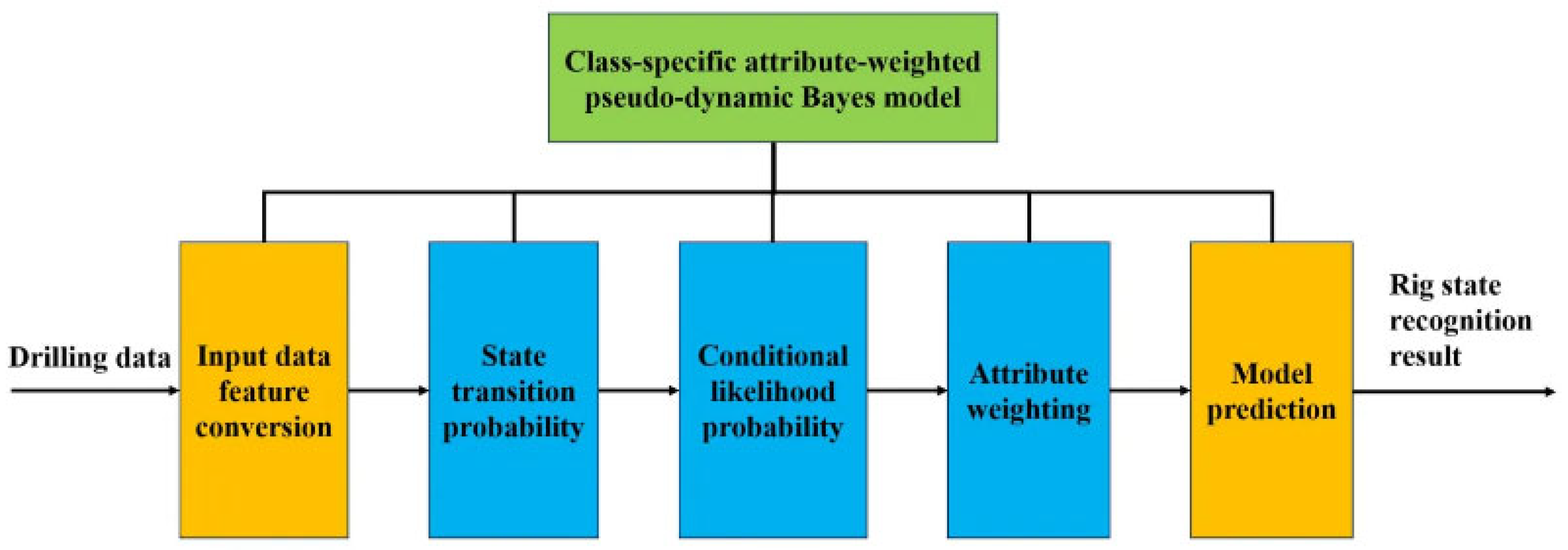
This section presents the development of a rig state classification model using the Class-specific Attribute-weighted Pseudo-Dynamic Bayes (CAWPDB) algorithm. Figure 1 illustrates the overall architecture of the proposed model, which consists of five main components. First, continuous drilling data undergo feature conversion to transform numerical measurements into categorical variables suitable for Bayes classification. Subsequently, the model development involves three core computational steps: determination of state transition probabilities based on domain expertise and training data, calculation of conditional likelihood probabilities from training data, and optimization of class-specific attribute weights. It should be noted that these computational steps are required only during the model training phase. Once trained, the model can directly classify rig states from converted input features, providing real-time operational state identification. The following subsections detail each component of this development process.

3.1. Data Preprocessing

Surface sensors record numerous drilling parameters. Including all measurements would not only increase model complexity but also potentially degrade classification performance. Consequently, we selected nine key parameters as input features: well depth, bit position, hook load, hook height, weight on bit, torque, rotational speed (RPM), standpipe pressure, and mud flow rate. The quality of training data is crucial for predictive accuracy. In this study, experienced drilling engineers labeled field-acquired sensor data according to established criteria, enabling development of an intelligent classifier that replicates expert decision-making in rig state identification. The training and testing datasets were mainly acquired from real-world horizontal well drilling operations in Bohai Bay, China, over the past three years. Data were collected from surface sensors at 10-s intervals during routine drilling operations.

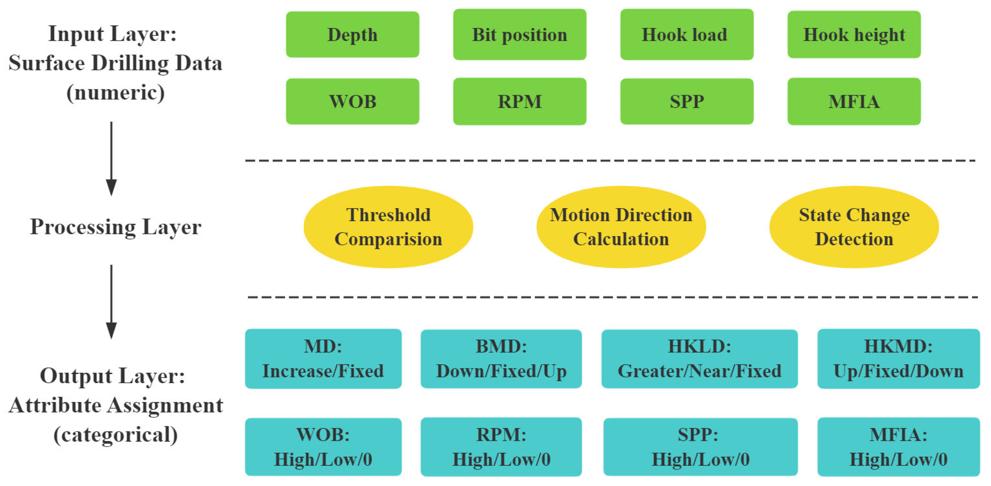
Prior to training, continuous drilling measurements were discretized into categorical variables. Figure 2 illustrates the complete workflow for converting numerical drilling data into categorical ranges.

Table 2. Training Data Samples for the Rig State Recognition Model.

MD	BMD	HKLD	HKMD	RPM	Torque	WOB	SPP	MFIA	Rig State
Fixed	Down	Greater	Down	High	High	0	Low	Low	RihRot
Increase	Down	Greater	Down	High	High	High	High	High	DrillRot
Fixed	Fixed	Fixed	Up	0	Low	0	0	0	InSlips
Fixed	Fixed	Greater	Fixed	Low	Low	0	0	0	Static
Fixed	Down	Greater	Down	Low	Low	0	Low	0	Rih
Fixed	Up	Greater	Up	Low	0	0	0	Low	Pooh
Fixed	Fixed	Fixed	Fixed	0	0	0	0	0	Null
Fixed	Down	Greater	Down	Low	Low	0	High	High	RihPump
Increase	Down	Greater	Down	Low	Low	High	High	High	DrillSlide
Fixed	Fixed	Greater	Fixed	High	High	0	Low	Low	StaticRot

presents representative training samples for the rig state recognition model. Columns 1–9 represent the input features: measured depth (MD), bit movement direction (BMD), hook load (HKLD), hook movement direction (HKMD), revolutions per minute (RPM), torque, weight on bit (WOB), standpipe pressure (SPP), and mud flow in rate (MFIA). These nine variables constitute a subset of the complete input features detailed in

Table 3. All Rig States and Attributes.

Rig States		Attributes	Attribute Values
		MD	Increase, Fixed
		BMD	Up, Fixed, Down
DrillRot	DrillSlide	HKLD	Greater, Near, Fixed
InSlips	DrillLine	HKMD	Up, Fixed, Down
Static	StaticPumpRot	RPM	High, Low, 0
StaticPump	StaticRot	Torque	High, Low, 0
Rih	Pooh	WOB	High, Low, 0
RihPumpRot	PoohPumpRot	SPP	High, Low, 0
RihRot	PoohRot	MFIA	High, Low, 0
RihPump	PoohPump	In well	Yes, No
Null	OutofSlips	HKLD change	Increase, Fixed, Decrease
		In bottom	Yes, No
		RPM change	Increase, Fixed, Decrease

.

Each feature was discretized into categorical values based on a systematic analysis of the training dataset combined with engineering principles. For example, statistical examination revealed that during effective drilling operations, WOB values ranged from 0 to 347 kN with a mean of 60.24 kN and median of 58.97 kN, while non-drilling states exhibited a range of 0–323 kN with a mean of 0.54 kN and median of 0 kN. Given that less than 1% of drilling samples showed WOB below 5 kN and less than 1% of non-drilling samples exceeded this value, 5 kN was selected as the threshold to distinguish “High” (>5 kN, indicating effective drilling) from “Low” (0–5 kN, transitional states) and “Zero” (≤0 kN, bit off-bottom). Negative values, occasionally observed due to overpull or sensor drift, were mapped to “Zero” as they physically represent non-drilling conditions. Similar data-driven thresholds were established for other parameters. Notably, sensors may register nonzero values for RPM, torque, SPP, or MFIA even when the drill string is stationary and mud pumps are inactive. Therefore, establishing appropriate thresholds is essential for filtering spurious measurements. The final column of Table 2 displays representative rig state labels, while Table 3 provides the comprehensive rig state taxonomy.

3.2. Development of the Pseudo-Dynamic Bayesian Model

In this section, a classifier capable of accurately identifying rig states based on drilling data will be developed using the Pseudo-Dynamic Bayesian algorithm. Training the Pseudo-Dynamic Bayesian classifier requires determining the state transition probability $P(c_{x-1},c_k)$ and the likelihood probability $P(a|c_k)$. The state transition probability $P(c_{x-1},c_k)$ is determined based on expert knowledge. For instance, given the previous class label $c_{x-1}$ as “DrillRot,” some of the state transition probabilities for the current class label $c_k$ are shown in

Table 4. Partial State Transition Probability Table.

	DrillRot	DrillSlide	InSlips	Rih	Pooh	RihPumpRot	PoohPumpRot
DrillRot	0.8	0.18	10−5	10−5	10−5	10−5	0.01

.

Based on the data in Table 1, the likelihood probability $P(a|c_k)$ is calculated using the following formula:

$$P(a|c_k)={\displaystyle \frac{N_{c_k,a}+1}{N_{c_k}+b}}$$

(3)

where $P(a|c_k)$ is the probability of the attribute value $a$ occurring given the class label $c_k$. $N_{c_k,a}$ is the number of samples in the training data where the class label is $c_k$ and the attribute value is $a$. $N_{c_k}$ is the total number of samples with the class label $c_k$. $b$ is the total number of possible values for the attribute to which $a$ belongs.

The partial likelihood probabilities for the attribute “HKMD” are shown in

Table 5. Partial Likelihood Probabilities $P(a|c_k)$ for the Attribute “HKMD”.

Operation	P (Up/Operation)	P (Fixed/Operation)	P (Down/Operation)
DrillRot	0.01	0.04	0.95
DrillSlide	0.005	0.025	0.97
InSlips	0.25	0.5	0.25
Rih	0.01	0.01	0.98
Pooh	0.987	0.01	0.003
RihPumpRot	0.002	0.02	0.978
PoohPumpRot	0.99	0.008	0.002

. These probabilities describe the likelihood of the hook moving upward, moving downward, or remaining stationary under a specific rig state.

Table 5 shows that, for the rotary-drilling state, the estimated probability of upward hook movement is extremely low but not exactly zero. This artifact arises because surface parameters are sampled at 10-s intervals, during which the rig may alternate between drilling and hoisting the drill string. With a sufficiently fine sampling rate, the probability of upward hook travel during pure rotary drilling would effectively be zero. Conversely, during the ‘Pooh’ state, the likelihood of downward hook motion similarly approaches zero, and analogous behavior is observed for other rig states.

Conditional likelihoods for all remaining attributes are calculated in the same manner from the training dataset.

3.3. Determination of Attribute Weights

Following the determination of state transition and likelihood probabilities, a Pseudo-Dynamic Bayes classifier is constructed. The next step involves establishing the class-specific attribute weight matrix.

For attribute weight optimization, this study employs the L-BFGS-B algorithm [17], a numerical optimization technique well-suited for high-dimensional nonlinear problems. This algorithm offers rapid convergence, computational robustness, and straightforward implementation. The optimization process minimizes the negative conditional log-likelihood as the objective function.

Class-specific attribute weighting requires determining significantly more parameters than global weighting methods. Although this increased parameterization enables the model to capture complex patterns and improve classification performance, it also raises the risk of overfitting [18]. To mitigate the risk of model overfitting, L2 regularization is applied by adding a penalty term $\lambda {\Vert w-w_1\Vert }^2$ to the objective function. Here, all elements of the $w_1$ matrix are initialized to 1, and the size of the $w_1$ matrix is the same as the $w$ matrix. The hyperparameter $\lambda$ is also initialized to 1. The regularization parameter $\lambda$ was set to 1 following standard practice in Bayesian classification literature, where this value typically provides reasonable regularization without excessive constraint on the weights. While systematic sensitivity analysis or cross-validation was not performed for $\lambda$ optimization, the model achieved excellent performance with this default setting, suggesting it was appropriate for this application. Future implementations could benefit from more rigorous hyperparameter tuning, though the computational cost of the iterative optimization process makes exhaustive search challenging. The objective function for minimizing the negative conditional log-likelihood is expressed as follows:

$$\begin{array}{ll}-CLL(w)& =-\log P(C|D,w)+\lambda {‖w-w_1‖}^2\\ & =-{\displaystyle \sum _{i=1}^n\log P(c_i|x_i,w)+}\lambda {‖w-w_1‖}^2\\ & =-{\displaystyle \sum _{i=1}^n\log \frac{P(c,x_i;w)}{{\displaystyle {\sum }_{c^{\prime }}(P(c^{\prime },x_i;w))}}}+\lambda {‖w-w_1‖}^2\end{array}$$

(4)

The specific process of weight optimization in the CAWPDB model is outlined as follows:

(1)

Initialization: Assign an initial weight of 1 to each attribute. Using the initialized weight matrix, along with the previously determined state transition probabilities and likelihood probabilities, construct the class-specific attribute-weighted pseudo-dynamic Bayes (CAWPDB) model.

(2)

Prediction: Apply the constructed model to predict each training sample. For each training sample $x_i$, calculate the posterior probability $P(c_i|x_i,w)$ under the weight matrix $w$, where $c_i$ represents the true class label.

(3)

Optimization: Substitute $P(c_i|x_i,w)$ into the conditional log-likelihood formula to compute the objective function. Employ the gradient descent method to minimize the negative conditional log-likelihood. Iteratively update the attribute weights until convergence or the maximum number of iterations is reached. Return the optimized attribute weight matrix upon completion of the optimization process.

The gradient calculation formula of $P(c,x_i;w)$ with respect to $w_{c,j}$ is as follows:

$$\begin{array}{ll}{\displaystyle \frac{\partial }{\partial w_{c,j}}}P(c,x_i;w)& =(P(c){\displaystyle \prod _{j^{\prime }\ne j}P{(a_{j^{\prime }}|c)}^{w_{c,j^{\prime }}}}){\displaystyle \frac{\partial }{\partial w_{c,j}}}P(a_j|c{)}^{w_{c,j}}\\ & =(P(c){\displaystyle \prod _{j^{\prime }\ne j}P{(a_{j^{\prime }}|c)}^{w_{c,j^{\prime }}}})P{a}_j|c{)}^{w_{c,j}}\log (P(a_j|c))\\ & =P(c,x_i;w)\log (P(a_j|c))\end{array}$$

(5)

The gradient calculation formula of $-CLL\left(w\right)$ with respect to $w_{c,j}$ is as follows:

$$\begin{array}{l}{\displaystyle \frac{\partial }{\partial w_{c,j}}}-CLL(w)\\ ={\displaystyle \frac{\partial }{\partial w_{c,j}}}{\displaystyle \sum _{i=1}^n\left[\log ({\displaystyle \sum _{c^{\prime }}P(c^{\prime },x_i;w})-\log (P(c,x_i;w))\right]}+2\lambda (w_{c,j}-1)\\ ={\displaystyle \sum _{i=1}^n\left[\frac{P(c,x_i;w)\log (P(a_j|c))}{{\displaystyle \sum _{c^{\prime }}P(c^{\prime },x_i;w)}}-\delta (c_i,c)\frac{P(c,x_i;w)\log (P(a_j|c))}{P(c,x_i;w)}\right]}+2\lambda (w_{c,j}-1)\\ ={\displaystyle \sum _{i=1}^n\left[P(c|x_i,w)\log (P(a_j|c))-\delta (c_i,c)\log (P(a_j|c))\right]}+2\lambda (w_{c,j}-1)\end{array}$$

(6)

The partially optimized weight matrix obtained is as

Table 6. Partial Optimized Attribute Weight Matrix.

	Attribute	MD	BMD	HKLD	HKMD	RPM	Torque	WOB	SPP	MFIA
State
DrillRot		0.92	0.82	0.72	0.61	0.93	0.92	0.94	0.80	0.60
DrillSlide		0.79	0.77	0.63	0.94	0.90	0.96	0.75	0.87	0.85
InSlips		0.83	0.70	0.65	0.92	0.67	0.66	0.78	0.78	0.72
Rih		0.84	0.57	0.76	0.95	0.94	0.65	0.63	0.68	0.91
Pooh		0.78	0.67	0.70	0.91	0.68	0.63	0.95	0.58	0.70
RihPumpRot		0.82	0.82	0.82	0.63	0.69	0.83	0.90	0.62	0.63
PoohPumpRot		0.78	0.84	0.75	0.62	0.82	0.95	0.93	0.82	0.65

:

While the attribute weights are mathematically optimized through the L-BFGS-B algorithm, the resulting weight patterns exhibit meaningful trends that align with drilling engineering principles. Rather than analyzing individual weight values, which represent complex interactions between multiple parameters, we focus on the broader patterns that emerge across different operational states.

The optimization process naturally groups attributes into three categories based on their relative importance across states. Primary mechanical indicators (RPM, WOB, torque) consistently show elevated weights for effective drilling states, reflecting their fundamental role in distinguishing drilling from non-drilling operations. Hydraulic and circulation parameters (SPP, MFIA) demonstrate moderate weights with higher variability across states, consistent with their state-dependent importance—critical during certain operations but less diagnostic for others. Positional and directional parameters (MD, BMD, HKLD, HKMD) show the widest weight distribution, ranging from highly significant in tripping operations to less critical during steady-state drilling, which aligns with operational practice where position monitoring intensity varies by operation type.

It is important to note that these weights represent relative importance within a multivariate classification framework rather than absolute physical relationships. The optimization algorithm adjusts weights to maximize classification accuracy while accounting for parameter correlations and redundancies. For instance, when multiple parameters provide similar diagnostic information, the algorithm may assign asymmetric weights to avoid over-relying on correlated features, which explains some of the non-intuitive weight variations observed.

The key insight is that despite being derived through mathematical optimization, the weight patterns broadly conform to drilling physics: mechanical parameters dominate during drilling operations, positional parameters become critical during tripping, and hydraulic parameters gain importance during circulation-dependent activities. This emergent alignment between data-driven optimization and domain knowledge validates the model’s physical reasonableness, even if individual weight values cannot be directly mapped to specific physical mechanisms. The model thus achieves a balance between mathematical rigor and engineering interpretability, making it suitable for field deployment where both accuracy and trustworthiness are essential.

4. Results and Analysis

4.1. Model Evaluation

The performance of the CAWPDB model is evaluated using four primary metrics: accuracy, precision, recall, and F1-score [19].

The classification performance of the developed CAWPDB model was evaluated using real surface drilling data from Well A. The collected data included over 58,000 data points, which were not used during model training, to test the model’s performance on unseen data.

Table 7. Classification Results of the Rig State Recognition Model on the Test Dataset.

Rig State (Class ${\mathit{C}}_{\mathit{k}}$)	$\mathit{T}{\mathit{P}}_{\mathit{k}}+\mathit{F}{\mathit{N}}_{\mathit{k}}$	$\mathit{T}{\mathit{P}}_{\mathit{k}}+\mathit{F}{\mathit{P}}_{\mathit{k}}$	$\mathit{T}{\mathit{P}}_{\mathit{k}}$	Precision (%)	Recall (%)	F1-Core (%)
DrillRot	25,000	25,000	25,000	100	100	100
InSlips	5020	5019	5017	99.960	99.940	99.950
Static	474	474	474	100	100	100
StaticPumpRot	1403	1407	1403	99.716	100	99.858
StaticPump	2675	2675	2675	100	100	100
StaticRot	140	140	140	100	100	100
Rih	1350	1351	1349	99.852	99.926	99.889
Pooh	46	46	46	100	100	100
RihPumpRot	5328	5327	5326	99.981	99.963	99.972
PoohPumpRot	16,539	16,537	16,537	100	99.988	99.994
RihPump	104	104	104	100	100	100
PoohPump	36	36	36	100	100	100
OutofSlips	288	287	287	100	99.653	99.826
Overall	Total number of instances		Number of correctly predicted instances		Accuracy (%)
	58,223		58,214		99.985

presents the experimental results of the proposed CAWPDB algorithm on the test dataset. In the table, $T{P}_k$ represents the number of instances correctly classified as class $C_k$, $F{P}_k$ represents the number of instances from other classes misclassified as class $C_k$, and $F{N}_k$ represents the number of instances from class $C_k$ misclassified as other classes.

The CAWPDB classifier achieved an overall accuracy of 99.985%, validating the effectiveness of the proposed approach. The model demonstrated consistently high precision, recall, and F1-score values across all rig state categories, confirming its robust performance and ability to accurately identify the vast majority of operational states while minimizing misclassifications.

Despite this exceptional performance, 0.0155% of test samples were misclassified. Several InSlips states were incorrectly identified as Rih states. These errors occurred during transitions from Rih to InSlips, when the drill string had not completely transferred its weight to the slips. This incomplete weight transfer resulted in slight upward hook movement and hook load readings exceeding elevator weight, causing the model to incorrectly classify these instances as Rih states. Additionally, some RihPumpRot and PoohPumpRot intervals were misclassified as StaticPumpRot. These errors occurred following StaticPumpRot sequences where minimal drill string movement fell below detection thresholds, resulting in negligible changes to hook height and bit position that led to incorrect StaticPumpRot classification.

These infrequent misclassifications do not diminish the model’s exceptional overall performance, which successfully identifies virtually all rig state transitions with high accuracy.

4.2. Comparison with Other ML Algorithms

The performance of the proposed CAWPDB classifier was benchmarked against both a Random Forest (RF) model and a standard Naive Bayes (NB) classifier. All three algorithms were trained on the dataset described in Section 3 and evaluated using the same surface drilling data from Well A. As shown in

Table 8. Comparison of Classification Results for Different Algorithms.

Model	RF			NB			CAWPDB
Rig State (Class ${\mathit{C}}_{\mathit{k}}$)	Precision (%)	Recall (%)	F1-Core (%)	Precision (%)	Recall (%)	F1-Core (%)	Precision (%)	Recall (%)	F1-Core (%)
DrillRot	99.94	99.94	99.94	99.91	99.96	99.94	100	100	100
InSlips	99.50	99.76	99.63	99.72	99.82	99.77	99.96	99.94	99.95
Static	92.61	97.89	95.18	97.87	97.05	97.46	100	100	100
StaticPumpRot	93.00	97.65	95.27	98.58	98.72	98.65	99.72	100	99.86
StaticPump	98.47	98.36	98.41	99.25	98.69	98.97	100	100	100
StaticRot	100	99.29	99.642	100	99.29	99.64	100	100	100
Rih	99.11	98.44	98.77	98.82	99.63	99.23	99.85	99.93	99.89
Pooh	90.91	65.22	75.95	89.74	76.09	82.35	100	100	100
RihPumpRot	97.86	95.25	96.54	98.82	99.27	99.05	99.98	99.96	99.97
PoohPumpRot	98.75	99.38	99.06	99.74	99.88	99.81	100	99.99	99.99
RihPump	55.56	19.23	28.57	88.46	44.23	58.97	100	100	100
PoohPump	63.64	38.89	48.28	55.26	58.33	56.76	100	100	100
OutofSlips	87.62	98.26	92.63	97.92	98.26	98.09	100	99.65	99.83
Overall	Accuracy (%)			Accuracy (%)			Accuracy (%)
	98.939			99.588			99.985

Abbreviations: RF, Random Forest; NB, Naive Bayes; CAWPDB, Class-Specific Attribute-Weighted Pseudo-Dynamic Bayes

, RF achieved an accuracy of 98.939%, compared with 99.588% for NB and 99.985% for CAWPDB. A detailed comparison of precision, recall, and F1-score across each rig state further demonstrates that CAWPDB consistently outperforms the other methods, delivering the highest metrics for the majority of states.

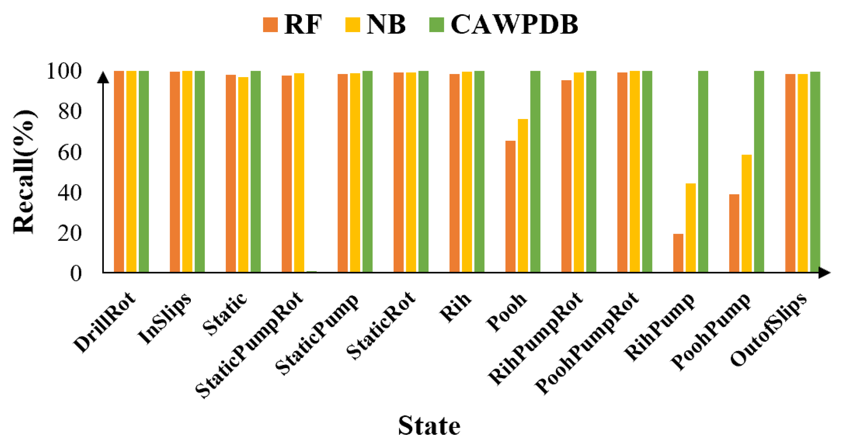
Despite their high overall accuracies, NB and RF struggle with infrequent rig states—such as “Pooh” and “PoohPump”—where their precision, recall, and F1-scores drop markedly below those of CAWPDB. Figure 3 illustrates the recall rates for each algorithm, highlighting how the inclusion of temporal dependencies in the CAWPDB model markedly improves classification accuracy for these low-frequency states.

5. Case Study: Connection Time Efficiency Analysis

This section demonstrates the practical application of rig state recognition for operational optimization. Using the CAWPDB model to classify rig states from surface data collected from two wells, we extract key performance indicators (KPIs) and quantify invisible lost time (ILT) to support drilling efficiency improvements. The two wells analyzed are horizontal development wells in the Bohai Bay and Sichuan Province, with total depths of 4473 m (Well A) and 5083 m (Well B). These wells are representative of typical development drilling in mature fields where operational efficiency directly impacts project economics.

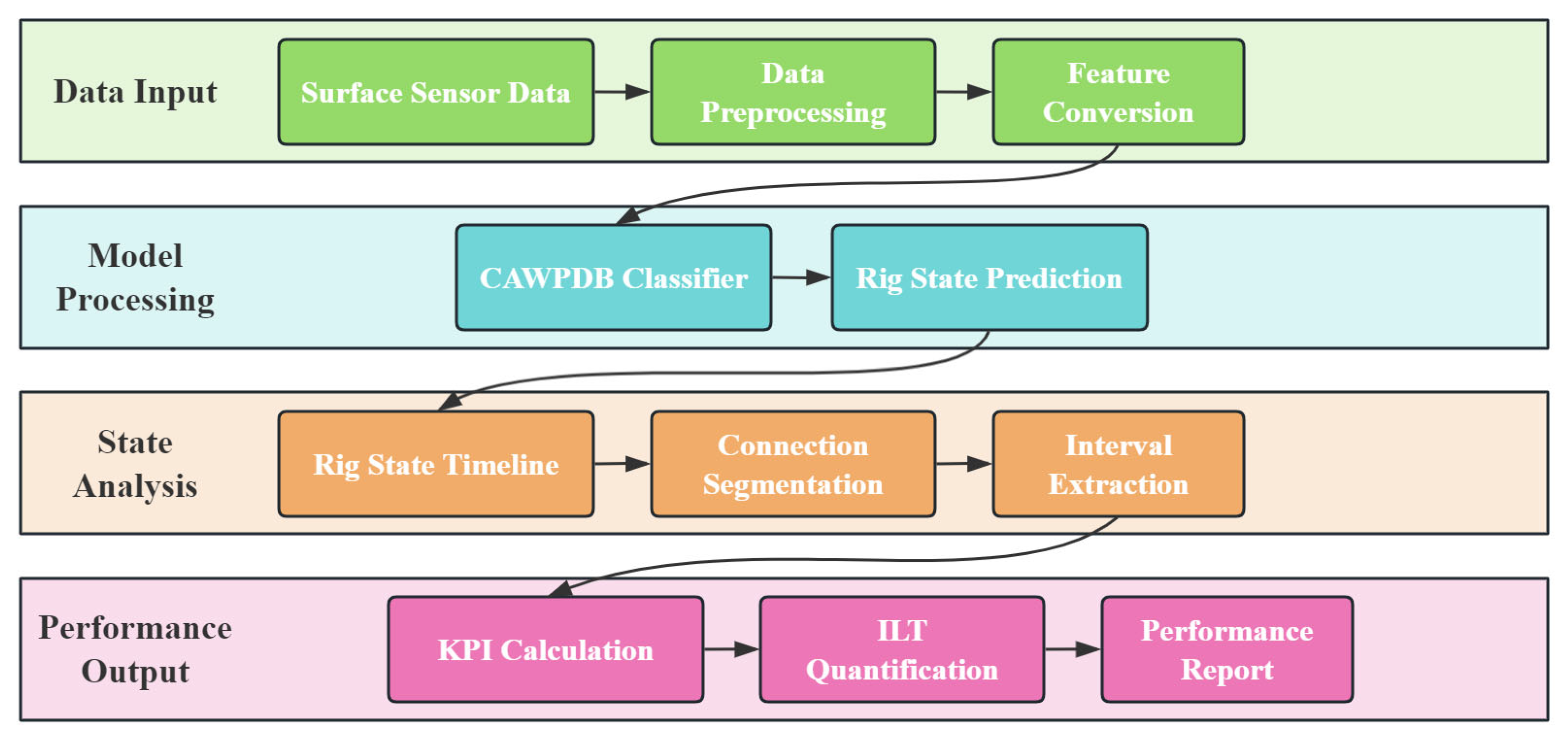
Figure 4 provides an overview of the complete workflow for drilling efficiency analysis using the CAWPDB model. The process begins with real-time drilling data acquisition, which is processed through the rig state classification model to generate a continuous rig state timeline. This timeline clearly delineates operational phases including drilling, reaming, back-reaming, and static operations. The classified states are then segmented into connection intervals—weight-to-slip, slip-to-slip, and slip-to-weight—enabling calculation of KPIs and quantification of ILT. This systematic approach transforms raw sensor data into actionable performance metrics for operational optimization.

5.1. Key Performance Indicator Assessment

Four KPIs were employed to evaluate drilling crew efficiency during connections: weight-to-weight, weight-to-slip, slip-to-slip, and slip-to-weight. When encountering potential stuck-pipe conditions, drillers may perform reaming or back-reaming operations to condition the wellbore before setting slips [20]. These preparatory activities—including reaming, back-reaming, and circulation—are incorporated into the weight-to-slip and slip-to-weight metrics [2].

The KPIs are defined as follows:

• Weight-to-slip: Elapsed time from lifting the bit off the bottom after drilling a stand to setting the drill string into slips. This interval may include operational states such as Static, RihPumpRot, PoohPumpRot, StaticPumpRot, Rih, and Pooh.
• Slip-to-slip: Duration between setting the drill string into slips and subsequently removing it, typically encompassing the Slip and DrillLine states.
• Slip-to-weight: Time required to run the drill string back to the bottom following slip removal. This interval can include states such as Static, RihPumpRot, PoohPumpRot, StaticPumpRot, Rih, and Pooh.
• Weight-to-weight: Total connection cycle time—from pulling the bit off the bottom after drilling a stand, through the full connection process, to returning the bit to the bottom. It is the sum of the weight-to-slip, slip-to-slip, and slip-to-weight intervals.

The rig state recognition model processes real-time surface measurements and classifies each time step into discrete operational states. For connection analysis, states between lifting off bottom and setting slips are aggregated into the weight-to-slip metric. Similarly, states from slip removal to returning to bottom constitute the slip-to-weight interval. The slip-to-slip interval includes only InSlips and DrillLine states. The sum of these three components yields the total weight-to-weight connection time.

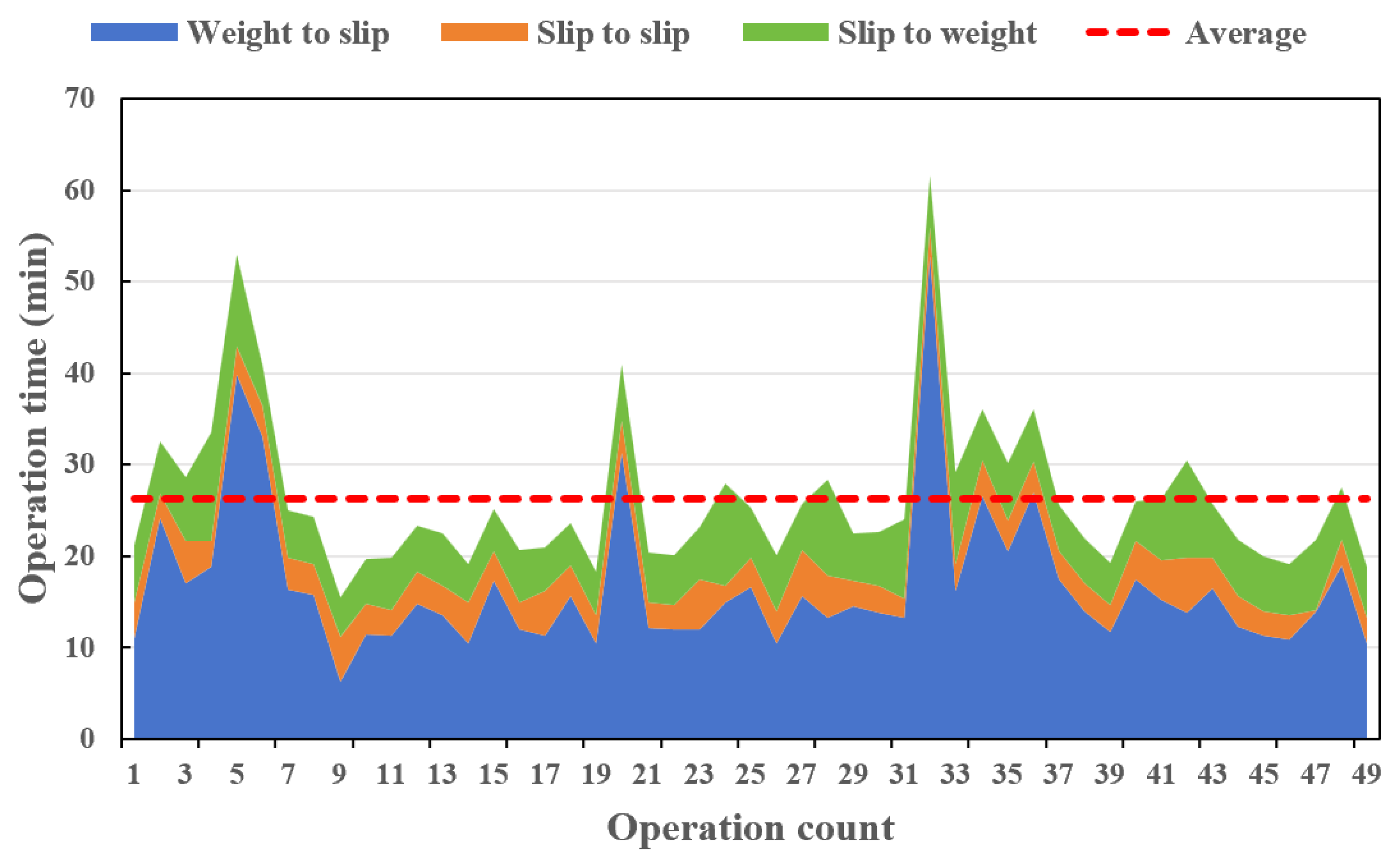
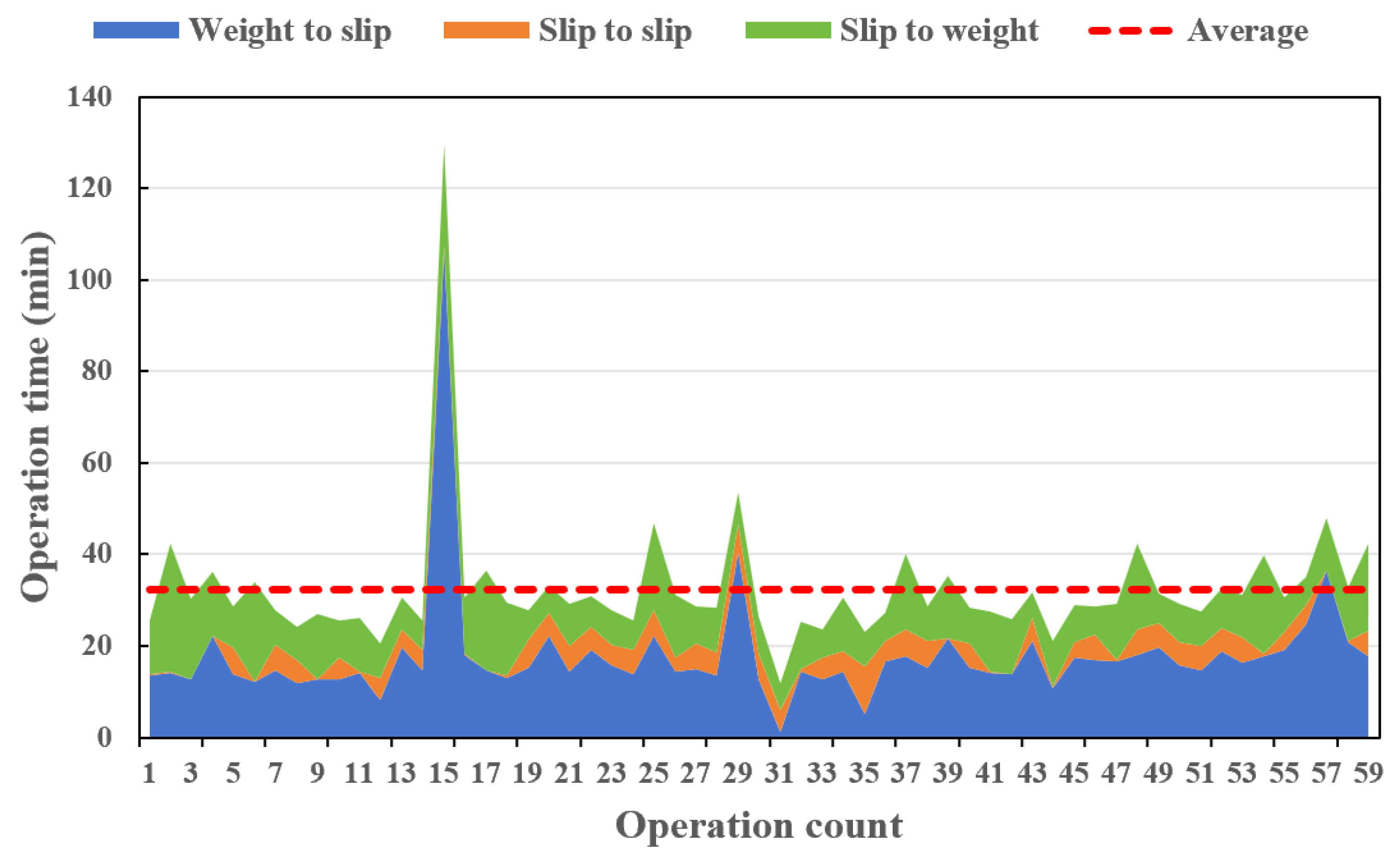
Figure 5 and Figure 6 display weight-to-weight connection times for two drilling crews. Figure 5 shows Crew A’s performance on Well A with an average connection time of 26 min, while Figure 6 presents Crew B on Well B averaging 32 min. These results reveal a distinct performance difference, with Crew A completing connections 23% faster than Crew B.

The integration of automated rig state identification with real-time monitoring enables immediate assessment of crew performance, providing actionable insights for operational optimization.

5.2. ILT Evaluation

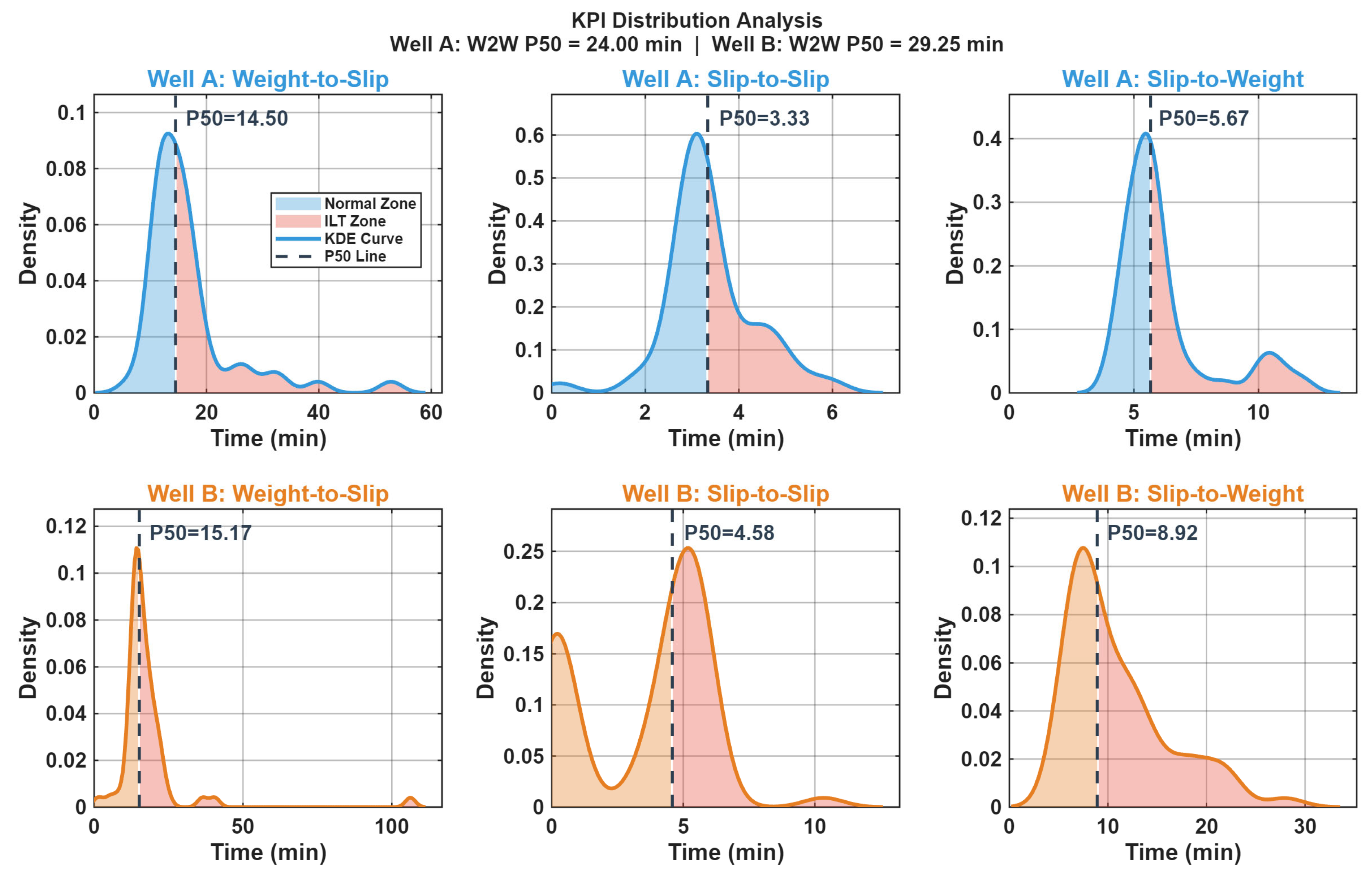
Prior to ILT calculation, establishing an appropriate weight-to-weight benchmark is essential for real-time KPI monitoring. This study employs the P50 method, using the median connection time as the optimal KPI threshold. Connection times exceeding this threshold are classified as ILT [21]. The 50th percentile provides a realistic, achievable target that maintains crew motivation while promoting continuous improvement.

For Well A, Figure 7 present the distributions of the weight-to-slip, slip-to-slip, and slip-to-weight KPIs. The respective P50 values are 14.50 min, 3.33 min, and 5.67 min, yielding an optimal weight-to-weight KPI of 24.00 min. For Well B, the P50 thresholds are 15.17 min for weight-to-slip, 4.58 min for slip-to-slip, and 8.92 min for slip-to-weight, resulting in an optimal weight-to-weight KPI of 29.25 min. ILT for each connection cycle is then calculated as the positive difference between the actual cycle time and the optimal KPI, allowing cumulative potential time savings to be quantified.

Table 9. Potential Time Savings Based on Optimal KPIs.

	Operation Time	KPI	Savings Potential Time	Savings Potential Time (%)
Well A	21 h, 27 min	24.00 min	1 h, 51 min	8.61%
Well B	31 h, 48 min	29.25 min	3 h, 3 min	9.57%
Total	53 h, 15 min	-	4 h, 54 min	9.18%

shows the time that can be saved if the operation times for the two wells tested are adjusted according to the optimal KPIs determined in this study. Using the P50 method, the total time saved is 4 h and 54 min, which accounts for 9.18% of the total operation time. The results demonstrate the effectiveness of the ILT measurement method based on rig state identification used in this study.

5.3. Economic Impact Assessment

The operational time savings identified through ILT analysis translate to significant economic benefits in offshore drilling operations. Based on current market data for shallow-water jack-up rigs in the Bohai Bay area, daily rates typically range from $80,000 to $120,000. For jack-up rigs specifically, though rates in domestic Chinese operations may be somewhat lower due to local market conditions. Using a conservative estimate of $100,000 per day for jack-up operations in Bohai Bay, the identified time savings yield substantial cost reductions. Total savings $20,417 for 4.9 h across both wells.

While these figures are lower than deepwater operations, they remain significant for shallow-water drilling economics. Considering that the CAWPDB implementation requires only software deployment with minimal hardware investment (estimated at <$5000 for system integration), the return on investment exceeds 400% for a two-well campaign.

For operators conducting multiple wells annually in mature fields like those in Bohai Bay, cumulative savings become substantial. A typical 10-well annual drilling program could potentially save 24.5 h, translating to approximately $102,083 in direct rig time savings. These calculations may exclude additional benefits. Furthermore, in the context of Bohai Bay’s mature field environment where margins are increasingly tight, even modest percentage improvements in drilling efficiency can significantly impact project economics and field development viability.

6. Discussion

The successful implementation of the CAWPDB model in field operations requires careful consideration of the human–machine interface and its integration with existing drilling workflows. Field personnel, particularly drillers and tool pushers, typically focus on immediate operational parameters rather than statistical analyses. Therefore, the system’s output has been designed to present actionable information through simple visual indicators rather than complex analytical metrics. Real-time KPI displays use color-coded alerts (green for efficient operations, yellow for marginal performance, red for significant deviations) that align with existing HSE visualization practices familiar to drilling crews. This approach ensures that even personnel without advanced data analytics training can immediately identify and respond to efficiency issues.

The closed-loop optimization mechanism operates through continuous feedback between rig state identification, performance monitoring, and operational adjustment. When the system detects connection times exceeding the P50 benchmark, it automatically generates specific recommendations based on the identified inefficiency source. For instance, if extended weight-to-slip times are detected due to excessive reaming, the system suggests optimal reaming parameters based on historical best practices from the same formation. These recommendations are displayed on the driller’s console as simple operational adjustments rather than abstract efficiency percentages.

This approach overcomes the traditional barrier between complex data analytics and practical field application. The real-time feedback created a “gamification” effect, where teams naturally competed to achieve better KPIs without requiring formal performance targets or management intervention. The system’s non-intrusive nature—operating passively without interfering with drilling operations—has been crucial for acceptance. Drillers maintain full control over operations while receiving data-driven suggestions that they can choose to implement based on their professional judgment and current drilling conditions.

To ensure sustainable adoption, the implementation follows a phased approach. Initially, the system operates in monitoring-only mode for allowing crews to become familiar with the displays without performance pressure. Training is integrated into regular safety meetings rather than requiring separate sessions, minimizing disruption to operations. Most significantly, the system’s benefits are communicated in terms relevant to field personnel: reduced physical workload through optimized operations, fewer stuck pipe incidents through efficient connections, and recognition for achieving best practices rather than criticism for inefficiencies. This human-centered approach is expected to naturally increase voluntary adoption rates and effectively enhance field operations, provided that it is properly adapted to the operational environment and workforce capabilities.

7. Conclusions

This study presents a novel rig-state classification model based on a class-specific attribute-weighted pseudo-dynamic Bayesian (CAWPDB) algorithm, delivering an overall accuracy of 99.985%. The following are the main findings that can be drawn from this study:

(1)

Drilling data exhibit inherent temporal dependencies. By incorporating expert knowledge into a state transition probability matrix, the pseudo-dynamic Bayes model effectively captures these temporal patterns while maintaining superior interpretability compared to conventional machine learning approaches.

(2)

Class-specific attribute weighting successfully addresses the conditional independence limitation of standard Naive Bayes. Benchmark comparisons demonstrate that CAWPDB significantly outperforms Random Forest and Naive Bayes classifiers, particularly for low-frequency rig states, achieving 99.985% overall accuracy.

(3)

Field application confirms CAWPDB’s reliability in identifying rig states from surface drilling data. The resulting classifications enable accurate KPI computation and ILT quantification, providing valuable metrics for crew performance evaluation and operational optimization.

(4)

While this study demonstrates CAWPDB’s effectiveness, several limitations suggest directions for future research. Future work should expand the dataset to improve probability estimates and validate model performance across diverse drilling environments to ensure broader applicability. The reliance on expert-defined state transition matrices, though ensuring interpretability, may limit scalability—future work should explore automated probability learning while maintaining domain knowledge integration. Additionally, developing online learning capabilities for real-time adaptation, improving robustness to sensor noise, and extending the framework to identify complex operational patterns represent promising research directions. Integration with automated drilling systems and transfer learning approaches could further enhance practical deployment across varied drilling operations.

(5)

The CAWPDB model’s Bayes framework, enhanced by expert-derived state transition matrices, enables effective classification with relatively limited training data compared to deep learning approaches. This characteristic makes the model particularly suitable for field deployment where comprehensive labeled datasets may be difficult to obtain, facilitating rapid implementation in new drilling operations.

References

1. Barakat, M.; Abu El Ela, M.; Khalaf, F. Integrating risk management concepts into the drilling non-productive time. J. Pet. Explor. Prod. 2021, 11, 887–900. [Google Scholar] [CrossRef] [Scilit]
2. Youcefi, M.R.; Boukredera, F.S.; Ghalem, K.; Hadjadj, A.; Ezenkwu, C.P. Development of an expert-informed rig state classifier using naive bayes algorithm for invisible loss time measurement. Appl. Intell. 2024, 54, 7659–7673. [Google Scholar] [CrossRef] [Scilit]
3. De Oliveira, G.L.; Zank, C.A.; Costa, A.F.; Mendes, H.M.; Henriques, L.F.; Mocelin, M.R.; de Oliveira Neto, J. Offshore drilling improvement through automating the rig state detection process-implementation process history and proven success. In Proceedings of the SPE/IADC Drilling Conference and Exhibition, Fort Worth, TX, USA, 1 March 2016; p. D031S024R006. [Google Scholar] [CrossRef] [Scilit]
4. Sun, T.; Zhao, Y.; Yang, J.; Yin, Q.; Wang, W.; Chen, Y. Real-Time Intelligent ldentification Method under Drilling Conditions Based on Support Vector Machine. Pet. Drill. Tech. 2019, 5, 28–33. [Google Scholar] [CrossRef]
5. Yin, Q.; Yang, J.; Cao, B.; Long, Y.; Chen, K.; Fan, Z.; He, X. Real-time intelligent rig activities classification model of deep-water drilling using Long Short-Term Memory (LSTM) network. Oil Drill. Prod. Technol. 2022, 1, 97–104. [Google Scholar] [CrossRef]
6. Ma, L. Drilling Condition Identification and Application Based on Logging Data. Master’s Thesis, China University of Petroleum, Beijing, China, 2023. [Google Scholar] [CrossRef]
7. Tran, T.; Pham, N.T.; Lundgren, J. A deep learning approach for detecting drill bit failures from a small sound dataset. Sci. Rep. 2022, 12, 9623. [Google Scholar] [CrossRef] [Scilit] [PubMed]
8. Ben, Y.; James, C.; Cao, D. Development and application of a real-time drilling state classification algorithm with machine learning. In Proceedings of the Unconventional Resources Technology Conference, Denver, CO, USA, 22–24 July 2019; Society of Exploration Geophysicists: Tulsa, OK, USA; pp. 3053–3066. [Google Scholar] [CrossRef] [Scilit]
9. Yin, Q.; Yang, J.; Hou, X.; Tyagi, M.; Zhou, X.; Cao, B.; Xu, D. Drilling performance improvement in offshore batch wells based on rig state classification using machine learning. J. Pet. Sci. Eng. 2020, 192, 107306. [Google Scholar] [CrossRef] [Scilit]
10. Murdoch, W.J.; Singh, C.; Kumbier, K.; Abbasi-Asl, R.; Yu, B. Definitions, methods, and applications in interpretable machine learning. Proc. Natl. Acad. Sci. USA 2019, 116, 22071–22080. [Google Scholar] [CrossRef] [Scilit] [PubMed]
11. Yang, X.; Zhang, Y.; Zhou, D.; Ji, Y.; Song, X.; Li, D.; Zhu, Z.; Wang, Z.; Liu, Z. Drilling conditions classification based on improved stacking ensemble learning. Energies 2023, 16, 5747. [Google Scholar] [CrossRef] [Scilit]
12. Zhang, W.J.; Jiang, L.X.; Zhang, H.; Hu, C. Bayesian classification learning framework based on bias-variance trade-off. Sci. Sin. Informationis 2023, 6, 1078–1095. [Google Scholar] [CrossRef] [Scilit]
13. Friedman, N.; Geiger, D.; Goldszmidt, M. Bayesian network classifiers. Mach. Learn. 1997, 29, 131–163. [Google Scholar] [CrossRef] [Scilit]
14. Zhang, H.; Sheng, S. Learning weighted naive Bayes with accurate ranking. In Proceedings of the Fourth IEEE International Conference on Data Mining, ICDM’04, Washington, DC, USA, 1–4 November 2004; IEEE: New York, NY, USA, 2004; pp. 567–570. [Google Scholar] [CrossRef] [Scilit]
15. Jiang, L.; Zhang, L.; Yu, L.; Wang, D. Class-specific attribute weighted naive Bayes. Pattern Recognit. 2019, 88, 321–330. [Google Scholar] [CrossRef] [Scilit]
16. Ghahramani, Z. Learning dynamic Bayesian networks. International School on Neural Networks; In Adaptive Processing of Sequences and Data Structures; Springer: Berlin/Heidelberg, Germany, 1997; pp. 168–197. [Google Scholar] [CrossRef] [Scilit]
17. Zhu, C.; Byrd, R.H.; Lu, P.; Nocedal, J. Algorithm 778: L-BFGS-B: Fortran subroutines for large-scale bound-constrained optimization. ACM Trans. Math. Softw. 1997, 23, 550–560. [Google Scholar] [CrossRef] [Scilit]
18. Zhang, H. Research on Fine-Grained AttributeWeighting Methods for Naive Bayes. Ph.D. Thesis, China University of Geosciences, Wuhan, China, 2023. [Google Scholar]
19. Mao, G.; Song, X.; Ding, Y.; Cui, M.; Liu, Y.; Zhu, Z. Drilling condition identification method based on gradient boosting decision tree. Oil Drill. Prod. Technol. 2023, 5, 532–539. [Google Scholar] [CrossRef]
20. Shokry, A.; Elgibaly, A.; Salem, A. Implementation of a novel eccentric dog leg reamer in oil well drilling. J. Pet. Explor. Prod. 2021, 11, 1199–1209. [Google Scholar] [CrossRef] [Scilit]
21. Raza, S.A.; Al-Braik, H.; Attalah, M.; Corona, M.; Kojadinovic, N. Performance enhancement of drilling and completions operations in giant offshore field Abu Dhabi by tracking and monitoring invisible lost time and defined KPIs. In Proceedings of the Abu Dhabi International Petroleum Exhibition and Conference, Abu Dhabi, United Arab Emirates, 13 November 2017; p. D011S020R002. [Google Scholar] [CrossRef] [Scilit]
Figure 1. Structural diagram of the CAWPDB model.
Processes 14 00405 g001
Figure 2. The procedure used for converting surface drilling data from numeric variables to categorical variables.
Processes 14 00405 g002
Figure 3. Comparison of Recall for Different Algorithms.
Processes 14 00405 g003
Figure 4. The workflow of drilling efficiency analysis.
Processes 14 00405 g004
Figure 5. Weight-to-weight time of Crew A in Well A.
Processes 14 00405 g005
Figure 6. Weight-to-weight time of Crew B in Well B.
Processes 14 00405 g006
Figure 7. KPI Distribution Analysis for Well A and Well B.
Processes 14 00405 g007