


Abstract
The economic dispatch (ED) problem is a major challenge in power system optimization. In this article, an Enhanced Social Group Optimization (ESGO) algorithm is presented for solving the economic dispatch problem with or without wind units, considering various characteristics related to valve-point effects, ramp-rate constraints, prohibited operating zones, and transmission power losses. The Social Group Optimization (SGO) algorithm models the social dynamics of individuals within a group—through mechanisms of collective learning, behavioral adaptation, and information exchange—and leverages these interactions to guide the population efficiently towards optimal solutions. ESGO extends SGO along three complementary directions: redefining the update relations of the original SGO, introducing stochastic operators into the heuristic mechanisms, and dynamically updating the generated solutions. These modifications aim to achieve a more robust balance between exploration and exploitation, enable flexible adaptation of search steps, and rapidly integrate improved-fitness solutions into the evolutionary process. ESGO is evaluated in six distinct cases, covering systems with 6, 40, 110, and 220 units, to demonstrate its ability to produce competitive solutions as well as its performance in terms of stability, convergence, and computational efficiency. The numerical results show that, in the vast majority of the analyzed cases, ESGO outperforms SGO and other known or improved metaheuristic algorithms in terms of cost and stability. It incorporates wind generation results at an operating cost reduction of approximately 10% compared to the thermal-only system, under the adopted linear wind power model. Moreover, relative to the size of the analyzed systems, ESGO exhibits a reduced average execution time and requires a small number of function evaluations to obtain competitive solutions.
1. Introduction
The economic dispatch (ED) problem represents a central component of operational optimization mechanisms in modern power systems, being employed to determine the optimal allocation of generation among available units such that the demand is met at minimum cost, while strictly satisfying the operational constraints of the generating units and the entire electricity transmission system [1,2].
In the current context, marked by the increasing penetration of renewable resources and by the pressure on operators to maintain economic competitiveness in a volatile environment, the analysis of the ED problem has become an indispensable tool for electricity producers [3]. The outcomes of such analyses directly influence operational strategies and production planning.
In the absence of wind integration, the ED problem exhibits a deterministic structure in which the technical parameters of conventional units (cost curves, operating limits, and ramp-rate constraints) allow a well-defined non-linear mathematical formulation, suitable for solution through classical optimization methods or metaheuristics [4]. Under these conditions, generation companies can rely on predictable system behavior, facilitating the establishment of efficient production schedules and strict control of marginal operating costs.
Several recent algorithms proposed for solving the classical ED problem are summarized below. The Hybridizing Gaining–Sharing Knowledge (GSK) and Differential Evolution (DE) approach is a hybrid method combining the global search ability of DE with the solution-refinement capacity of GSK [5]. The Exponential Hybrid Mutation Differential Evolution (EHMDE) introduces two key strategies—exponential population-size reduction and a hybrid mutation operator—designed to balance exploration and exploitation during optimization [6]. The Hybrid Gray Wolf Optimization (HGWO) algorithm integrates a robust learning mechanism intended to prevent the stagnation of search agents in suboptimal regions [7]. The Growth Optimizer is a recent metaheuristic that inspires individuals to enhance their capabilities through learning and reflection as they evolve within society [8]. The Improved Pelican Optimization Algorithm introduces strategies that more accurately model more the stochastic hunting behavior of pelicans [9]. The Enhanced Social Network Search (ESNS) algorithm improves the original version by increasing search intensity around promising solutions, enhancing exploration, and avoiding entrapment in local minima [4]. The Leader White Shark Optimization algorithm incorporates a leadership mechanism aimed at intensifying exploitation and improving the efficiency of ED problem solving [10]. The Wild Horse Optimizer is a new metaheuristic designed to be simple to implement and to exhibit rapid convergence when applied to the ED problem [11]. The Enhanced Manta Ray Foraging Optimization method provides improved search mechanisms for ED systems of various sizes and characteristics [12]. Finally, the Memetic Salp Swarm Algorithm is a hybrid method that employs an adaptive β-hill climbing strategy for local search [13].
Integrating wind generation into power systems fundamentally alters the ED architecture. The variability of wind power output and the inherent uncertainty of meteorological forecasts require additional probabilistic modeling instruments capable of characterizing wind speed fluctuations in a rigorous manner [14]. For power companies, this extension introduces opportunities associated with cost reduction through the utilization of a resource with a very low marginal production cost. Mathematically, the inclusion of wind generation significantly increases the complexity of the ED problem, as the interaction between uncertainty and the optimal decision becomes a key determinant. The objective function involves multiple terms (e.g., fuel costs, penalties for forecast deviations), reflecting the operational realities of generating companies.
Several mathematical optimization models and appropriate solution algorithms have been proposed in the literature for ED problems that include wind power uncertainty. For example, Ref. [14] introduces a model that extends the classical ED formulation by integrating wind farms into the power system, where wind speed is represented by a Weibull distribution. In addition to fuel cost, the model includes specific penalties for wind power overestimation and underestimation, thus explicitly addressing the risks associated with fluctuating production. Compared to [14], the studies in [15,16] incorporate an additional objective term reflecting emission costs due to thermal unit operation. Optimization for wind–thermal power systems is performed using Quantum-Inspired Particle Swarm Optimization [15] and Gbest-Guided Artificial Bee Colony [16].
In [17], the ED problem with wind integration is solved using the Honey Bee Mating Optimization algorithm with an embedded online learning mechanism, where wind-speed uncertainty is estimated using the 2 m-point method.
The study in [18] applies the Lagrange multiplier method to several power systems (6-unit, 10-unit, and 40-unit) with various demand levels, modeling wind speed through a Weibull distribution. The Fractal Firefly Algorithm is proposed in [19] for allocating generation among thermal and wind units under constraints such as unit capacity limits, power balance, multi-fuel operation, and ramp-rate limitations.
In [20], the authors introduce a hybrid algorithm based on Particle Swarm Optimization (PSO) operating in a scenario-based framework in which wind generation uncertainty is represented through multiple probabilistic scenarios. The method combines enhanced exploration mechanisms with robust selection strategies to ensure that the obtained solutions remain effective under varying wind conditions. Numerical results show that the proposed method achieves lower operating costs and improved convergence stability compared with standard PSO and other existing methods.
An economic dispatch model focusing on the management of wind generation uncertainty is described in [21]. To ensure computational efficiency, the authors employ an Alternating Direction Method of Multipliers (ADMM) combined with a Finite-Step Consensus strategy.
In [3], the authors formulate a probabilistic-constraint ED model and propose a hybrid optimization method that integrates chaotic maps into the Artificial Bee Colony (ABC) algorithm to enhance search diversification and prevent premature convergence—key aspects when dealing with the inherent variability of wind resources. Comparative experiments on test systems (10-unit, 40-unit) demonstrate that the proposed method reduces total operating cost and improves convergence stability relative to classical ABC and other metaheuristics.
In computational intelligence, the modeling of collective and cognitive processes has proven to be a powerful paradigm for developing robust optimization techniques. This is evident across diverse domains, from structural advancements in brain–machine contextual communication [22] to the design of swarm- and social-based metaheuristics. The Social Group Optimization (SGO) algorithm [23] is part of this paradigm, being inspired by the dynamics of social interactions within human groups. It models individual behavior through mechanisms such as social learning, cooperation, and context-based adaptation, aiming to achieve an effective balance between exploration and exploitation of the search space.
The authors propose a solution-update process based on the influence of leaders and information exchange among group members. Tested on an extensive set of benchmark functions, SGO has demonstrated competitive performance relative to established metaheuristics (ABC, PSO, DE, and TLBO), highlighting its potential for global optimization. However, the standard SGO version exhibits several limitations, such as a tendency to stagnate in local optima [24], loss of population diversity [25], low sensitivity to decision-variable changes [25], and reduced stability for large-scale optimization problems [26]. These shortcomings indicate that the algorithm cannot be universally applied without adaptation, as its performance becomes limited in many contexts. The limitations highlighted for the standard version of the SGO algorithm are not isolated, but rather belong to a broader set of challenges characteristic of population-based metaheuristic algorithms. Phenomena such as early search bias toward suboptimal solutions, progressive loss of population diversity, or reduced responsiveness to variations in decision variables are frequently reported in the specialized literature for algorithms inspired by collective behaviors. In this context, improving solution-update mechanisms and search-step generation strategies represents an essential direction for increasing the efficiency of the optimization process.
To overcome these limitations, various SGO variants have been developed, targeting the following: (i) enhanced exploration–exploitation capability using a Self-Perception Probability (SAP) mechanism in the acquiring phase [27]; (ii) reduction in local stagnation by integrating chaotic maps [28]; (iii) dynamic adjustment of the exploration–exploitation balance via an adaptive inertia parameter controlled by a sigmoid function [29]; (iv) maintaining population diversity through new heuristics embedded in the improving phase [30]; and (v) achieving more robust balance through hybridizations with WOA [25] or DE [31]. In this context, the proposed ESGO variant is designed to overcome the limitations of a simple local adjustment of the SGO algorithm through an approach aimed at improving the global behavior of the search process. The introduced modifications seek to support a more effective exploration–exploitation balance, preserve population diversity, and increase the stability of the optimization process. Thus, ESGO provides a strengthened framework for addressing complex optimization problems, and its usefulness is demonstrated in this work in the context of the ED problem.
In this article, to enhance SGO’s ability to identify high-quality and stable solutions for the ED problem, we develop a new variant of the algorithm, denoted Enhanced SGO (ESGO). ESGO introduces a set of restructured heuristics relative to those in SGO, as well as new stochastic operators designed to generate more effective search steps, leading to superior solutions and lower overall costs compared to the traditional SGO.
The main contributions of this article are summarized below:
- (i)
- A new version of the SGO algorithm, denoted ESGO, in which the heuristics used for solution updates have been modified to enable searching both in the vicinity of the best solution (in the improving and acquiring phases) and around the current solution (in the acquiring phase). In the acquiring phase, activation of a heuristic is determined through a double conditioning based on the fitness value and a randomly generated number. Additionally, to obtain appropriate search steps, heuristics incorporate stochastic operators based on combinations of uniformly distributed and Cauchy-distributed random numbers. To the best of the authors’ knowledge, the Cauchy distribution has not previously been integrated into the SGO structure.
- (ii)
- Implementation of ESGO for solving the economic dispatch (ED) problem, considering various practical characteristics, including the presence of wind units.
- (iii)
- Evaluation of ESGO’s feasibility and efficiency for the ED problem on multiple power system configurations (6-unit, 40-unit, 110-unit, and 220-unit). Furthermore, the Wilcoxon nonparametric statistical test is used to determine whether significant differences exist between ESGO and SGO across the analyzed test cases. The results show that ESGO outperforms SGO and other benchmark algorithms reported in the literature for solving the ED problem.
The structure of the article is organized as follows. Section 2 presents the mathematical optimization model of the ED problem, with and without wind integration. Section 3 describes the structure and heuristics underpinning the SGO algorithm. Section 4 details the enhanced ESGO version. Section 5 explains how ESGO is implemented for the ED problem, with or without wind integration. Section 6 presents the analyzed cases and the numerical results obtained by SGO, ESGO, and other reference algorithms. The conclusions are summarized in Section 7.
2. Statement of the ED Problem
We consider a power system in which both thermal units and wind units coexist. The economic dispatch (ED) problem consists of determining an optimal generation schedule for each generating unit such that the total operating cost is minimized, the power demand is fully supplied over the scheduling horizon, and the technical limits of the units and of the system are satisfied.
For the mathematical formulation of the optimization model, we assume that the system includes n = t + w units, where t is the number of thermal units and w is the number of wind units. The power outputs of all units are stored in the vector P = [W, T] = [P1, P2, …, Pj, …, Pn], which is composed of the vectors W and T, where W = [W1, W2, …, Wq, …, Ww] and T = [T1, T2, …, Tk, …, Tt] represent the power output vectors of the wind and thermal units, respectively. The total operating cost (Cost), which defines the objective function for the ED problem, is composed of the cost associated with the thermal units, (CostThermal) and the cost associated with the wind units (CostWind):
These two types of costs can be defined as follows [14,32]:
where ak, bk, ck, ek, and fk are the fuel cost coefficients of thermal unit k; Tk,min is the minimum generation capacity of thermal unit k; , represent the average power corresponding to the overestimation and, respectively, underestimation of wind power of unit q; dq, oq, and uq are the direct cost, overestimation, and underestimation coefficients for q unit.
The production of the thermal units is associated with the fuel cost for each unit k—CostTk(Tk), modeled by the non-convex fuel cost function in (2). The wind power generation of unit q involves an aggregated cost—CostWq(Wq) that includes the following [14]: direct operating costs—the term dq·Wq in relation (3), overestimation penalty costs—modeled by the term , and underestimation penalty costs—modeled by The penalty costs are average costs introduced to model the mismatch between the scheduled and the actual power output of each wind unit q. Thus, overestimation occurs when the scheduled power level for a wind unit is higher than the power that the unit can effectively deliver, given the available wind resource and the forecasted wind conditions at the site; underestimation occurs when the scheduled power is lower than the power available from the wind resource. Equations (2) and (3) are among the most widely used models for defining the costs associated with thermal and wind units and provide good accuracy.
The average powers and are determined considering the probability distribution of the random variable wind power (W), which depends on the random variable wind speed (V). In this work, we assume that V follows a Weibull distribution with probability density function fV(v) given by (5), while the relationship between V and W is assumed to be linear [16]:
where k and c are the shape and the scale parameter, respectively, and v is a value of the random variable V.
The functional relationship W = f(V) explicitly defined in (4) requires the knowledge of the wind speed characteristics for a given location: vin (cut-in wind speed, representing the minimum wind speed required for turbine operation), vr (rated wind speed—speed at which turbine reaches maximum power), and vout (cut-out wind speed—maximum safe operating speed), as well as the rated power (Wr) of the wind unit. Within the operating range vin ≤ V ≤ vr, a linear relationship between wind speed and generated power is assumed. This approximation is commonly adopted in economic dispatch studies to reduce model complexity and computational burden. However, since actual wind turbine power curves are inherently non-linear, this assumption may introduce estimation errors, particularly under high wind penetration levels, which can affect the accuracy of dispatch results.
Given that the wind speed at the site of wind unit q follows a Weibull distribution, the average powers and can be calculated as follows [14]:
where w are the possible values of the random variable wind power Wq, and is the probability density function for Wq. Since the distribution of V is known and the relation W = f(V) is given, the probability density function fW(w) of the wind power W can be obtained as follows:
where R = (vr − vin)/vin.
Prob(Wq = 0) represents the probability that the wind power Wq is equal to zero, i.e., the probability that the wind speed is either less than or greater than [14]:
Prob (Wq = 0) = Prob (V < vin) + Prob (V > vout) = 1 − exp[−(vin/c)k]+ exp[−(vout/c)k]
Prob(Wq = Wrq) is the probability that the wind power of unit q equals its rated capacity Wq, i.e., the probability that the wind speed V lies between vr and vout [14]:
Prob(W = Wrq) = Prob(vr < V < vout) = exp[−(vr/c)k] − exp[−(vout/c)k]
The set of constraints imposed on the ED problem including wind power is as following [15]:
where (11) defines the minimum (Tk,min) and maximum (Tk,max) power limits of thermal unit k. Similarly, the power outputs of the wind units Wq are bounded by a lower limit (Wq,min) and upper limit (Wq,max), as in (12). If the power output () of thermal unit k in the previous hour is imposed, then its operating limits are further restricted by (13), where DRk and URk are the down-ramp and up-ramp limits of the unit k. An additional type of constraint for the generating units refers to prohibited operating zones (POZ), described mathematically by (14). POZs are power intervals in which unit operation is not allowed due to technical reasons, such as mechanical vibrations, resonance phenomena, thermal instabilities, or significant efficiency degradation. The limits Pk,zinf and Pk,zsup represent the lower and upper bounds of the prohibited zone z for unit t, while nzk represents the number of prohibited zones of unit t.
Tk,min ≤ Tk ≤ Tk,max, k = 1, 2, …, t
Wq,min ≤ Wq ≤ Wq,max, q = 1, 2, …, w
Additionally, at system level, the power balance between generated power (PG) from thermal and wind units, demanded power (PD), and power losses (PL) must be maintained:
The transmission losses PL can be calculated using the B coefficient loss formula (Kron’s formula):
where Bij, B0j, and B00 are constant and known loss coefficients for a given load level. For a candidate solution vector [P], the satisfaction of the equality constraint (15) is achieved with less accuracy than an imposed ε:
Accuracy = |PG − PL − PD| < ε
3. Social Group Optimization (SGO)
Social Group Optimization (SGO) is a metaheuristic algorithm inspired by human social behavior, proposed for solving complex optimization problems and various engineering applications by Satapathy and Naik [23]. The basic philosophy of SGO is founded on the observation that individuals within a social group tend to improve their behavior based on interactions with other members of the group.
The essential elements of the social group are the number of individuals in the group, denoted by (N), and the set of traits associated with each individual, denoted by (n). Within the social group, the following associations are established: individuals in the social group are associated with candidate solutions, Xi, i = 1, 2, …, N, the traits of the individuals correspond to the components xij, j = 1, 2, …, n of solution Xi = [x1,i, x2,i, …, xj,i, …, xn,i], and the knowledge accumulated by individuals is associated with the fitness function, f(Xi).
The SGO algorithm starts with an initialization phase in which the traits of the individuals xj are generated randomly between the lower bounds (Xmin = [x1,min, x2,min, …, xj,min, …, xn,min]) and upper bounds (Xmax = [x1,max, x2,max, …, xj,max, …, xn,max]) imposed by the problem. The update of the individuals’ traits is carried out in two successive phases. Improving phase—the best individual in the group (Xbest) attempts to transfer their knowledge to the other members (Xi, i = 1, 2, …, N) in order to help them improve their knowledge base. Acquiring phase—the traits of each individual Xi are updated to a new solution Xi,new based on the interaction among three individuals: the current individual Xi, the best individual in the group Xbest o, and a randomly selected individual Xr, r ≠ i. The mathematical modeling of these concepts in the three phases is given by relations (18)–(20) [23]:
where Xi,new is the new solution obtained by updating Xi using (19) or (20); Xbest is the best solution up to that point (the individual with the best traits/knowledge); for a minimization problem, Xbest corresponds to min{fi,i = 1, 2, …, N}. Xr is a randomly selected solution from the group, r ≠ i; Xmin and Xmax are the imposed lower and upper bounds; c is the self-introspection factor (0 < c < 1); r1, r2, r3, and r4 are random numbers uniformly distributed in the interval (0, 1).
The execution of the SGO algorithm stops when the maximum number of iterations, tmax, is reached. The best solution (Xbest) and its associated fitness value f(Xbest) are then recorded. A pseudo-code of the SGO algorithm is given below in Algorithm 1 [23].
| Algorithm 1: SGO algorithm |
| Set: the population size (N), maximum number of iterations (tmax) {Initialization phase} Initialize solutions Xi, i = 1, 2, …, N using (18) Evaluate fitness f(Xi), then identify Xbest, and f(Xbest) while t ≤ tmax for i = 1 to N do {Improving phase} Update Xi,new by relation (19), then evaluate f(Xi,new) Accept Xi,new if it has a better fitness end for Identify Xbest, and f(Xbest) in the current population for i = 1 to N do {Acquiring phase} Randomly select a solution Xr, r ≠ i Update Xi,new using (20a), or (20b) Evaluate f(Xi,new) Accept Xi,new if it has a better fitness end for Identify Xbest, and f(Xbest) from the population t = t + 1 end while Store Xbest, and the fitness f(Xbest). |
4. Enhanced SGO (ESGO)
The proposed Enhanced SGO (ESGO) algorithm preserves the overall structure and evolutionary steps of the original SGO algorithm; however, several internal mechanisms of SGO are modified in order to increase the global efficiency of ESGO. In its classical form, the SGO algorithm performs the solution update through search steps whose values are controlled exclusively by random variables r1–r4, generated uniformly in the interval (0, 1), according to relations (19) and (20). While this strategy favors diversity and exploration of the search space, its efficiency can be limited for problems with high complexity, such as those where the objective function has many local minima and/or a high dimensionality of variables. Therefore, the exploration–exploitation balance may not be adequate, potentially leading to stagnation in local minima or inconsistent solution quality.
To improve the search process in ESGO compared to the traditional SGO, three directions are followed: modification of the update relations for the solutions (heuristics); inclusion of random operators within the heuristics; and dynamic update of the obtained solutions. Each direction targets a specific objective. Thus, modifying the solution-update relations aims to achieve a better exploration–exploitation balance during the search (avoiding stagnation and obtaining more refined solutions). Including random operators in the heuristics is intended to produce search steps with appropriate amplitude and direction. Dynamically updating improved solutions aims to introduce better candidate solutions into the search process as quickly as possible. Concretely, the improvements introduced in ESGO with respect to SGO are as follows:
- (i).
- In the improving phase, the relation (19) of SGO is replaced by (21) in ESGO:
- (ii).
- In the acquiring phase, relations (20) are replaced by (22) and (23) in ESGO:
The probability density function f(x) and the distribution function F(x) for the Cauchy distribution are defined as follows:
where x0 is the location parameter and s is the scale parameter.
Figure 1 illustrates the shape of the Cauchy distribution for x0 = 0 and different values of the scale parameter: very small (s = 0.01), moderately small (s = 0.1), and relatively large (s = 1). From Figure 1, it can be observed that the Cauchy distribution is symmetric and can generate positive and negative values with higher probability when the value of the parameter s increases. This behavior can be exploited to control the amplitude and direction of the computational steps in the heuristic relations (21)–(23).
Figure 1.
Function f(x) for Cauchy distribution.
- (iii).
- In ESGO, the uniformly distributed random variables r2–r4, used in the original SGO algorithm, are replaced by explicitly defined random operators that are directly embedded in the solution-update relations (21)–(23). In this work, a random operator is defined as a stochastic component with a specific mathematical form that provides explicit control over the scaling and/or sign of the search step, while the geometric orientation of the step is determined by the vector differences between candidate solutions. Three types of explicitly defined random operators are employed:
- (a)
- Uniform random operator rand(0, 1), which introduces stochastic scaling of the update step;
- (b)
- Trigonometric random operator sin(rand(0, 2π)) or cos(rand(0, 2π)), whose absolute value controls the step magnitude, while its sign may reverse the orientation of the displacement along a given reference direction;
- (c)
- Cauchy-based random operator rChy(0, s), which generates heavy-tailed random values symmetrically distributed around zero. Due to its sign and magnitude, this operator can both amplify or attenuate the step length and invert its direction. The scale of these variations is adaptively regulated by the parameter s, which decreases linearly from b to a (b > a > 0) over the iterations, thereby progressively limiting large-amplitude steps and enabling a smooth transition from exploration to exploitation.
In the update relations (21)–(23), the vector differences, such as (Xbest − Xi) and (Xi − Xr), define the reference geometric directions of movement and contribute implicitly to the step magnitude through their norms. The explicitly defined random operators act multiplicatively on these vectors and are responsible for the stochastic regulation of the effective step size and, in some cases, of the direction sign. In relation (21), a composite random operator rand(0, 1)⋅rChy(0, s) is employed to adaptively scale the displacement toward the current best solution, guiding the search process in the direction of Xbest. In the acquiring phase, alternative update heuristics given by relations (22a)–(22b) and (23a)–(23b) are selected stochastically according to the condition rand(0, 1) < 0.5, enabling random switching between locally and globally oriented search behaviors. This combination of explicitly defined random operators and stochastic heuristic selection ensures a balanced and adaptive exploration–exploitation process.
Applying the inverse transformation method to relation (25), we obtain the procedure for generating a random number from a Cauchy distribution with fixed parameters x0 and s:
where u is a random number uniformly distributed in the interval (0, 1), and tan(·) is the tangent trigonometric function.
In this work, the parameter x0 is set to x0 = 0 (to allow the generation of both positive and negative values with equal probability of 50%), while s decreases linearly from β to α (β > α > 0) depending on the current iteration index t and the maximum number of iterations tmax:
According to relation (27), in the early iterations of the optimization process, the parameter s of the Cauchy distribution takes relatively high values, close to β, which favors the exploration phase of the search space. As the iterative process evolves, the value of s decreases, favoring the exploitation phase. Thus, incorporating the Cauchy distribution into the heuristics allows both exploration and exploitation phases to be carried out, as well as a gradual transition from “predominantly exploration” to “predominantly exploitation”. Figure 2 highlights the points generated by the Cauchy distribution for moderate values of the parameter s (s = 0.1, shown by the plot of rChy(0, 0.1)—green points) and for higher values (s = 1, shown by the plot of rChy(0, 1)—blue points). It can be observed that for s = 0.1, the generated values are concentrated close to the origin, x0 = 0, while for s = 1, they exhibit a much larger spread.
Figure 2.
Values generated by rChy(0, 0.1) and rChy(0, 1).
- (iv).
- At each update of the solutions obtained using relations (21)–(23), a greedy process is applied between Xi (the old solution) and Xi,new (the new solution) to select and retain the solution with the better fitness value. The same procedure is used when selecting the best solution (Xbest) generated up to the current moment.
- (v).
- In ESGO, the parameter c is eliminated, and two new parameters (α, β) are introduced, which must be adjusted to increase the performance of the proposed algorithm.
The computational steps for implementing the proposed ESGO are presented in Algorithm 2.
| Algorithm 2: ESGO algorithm |
| Set the parameters for ESGO: N, tmax, α, β {Initialization phase} Initialize solutions Xi, i = 1, 2, …, N using relation (18) Evaluate the fitness f(Xi), then identify Xbest, and f(Xbest) while t ≤ tmax for i = 1 to N do {Improving phase} Update ≤ the s parameter using relation (27) Generate a random number, rChy(0, s), based on relation (26) Update Xi,new using relation (21), then evaluate the fitness f(Xi,new) Update Xi, and XBest, (and correspondingly f(Xi), and f(XBest)) if the new solution has better fitness end for for i = 1 to N do {Acquiring phase} Randomly select a solution Xr, i ≠ r Update the parameter s using relation (27) Generate a random number, rChy(0, s), based on relation (26) If f(Xi) < f(Xr) Then update Xi,new using relations (22a) and (22b) Else update Xi,new using relations (23a) and (23b) Update Xi, and XBest, (and correspondingly f(Xi), and f(XBest)) if the new solution has a better fitness end for t = t + 1 end while Store Xbest, and the fitness f(Xbest). |
5. Implementing the ESGO for the ED Problem
We consider that a solution i of the ED problem is represented by the power vector Pi = [Wi, Ti] = [[W1i, W2i, …, Wqi, …, Wwi] [T1i, T2i, …, Tki, …, Tti]] = [P1,i, P2,i, …, Pj,i, …, Pn,i], n = t + w, i = 1, 2, …, N. The vector Pi thus contains the power outputs of both wind units and thermal units (the first w components correspond to the wind units, while the remaining t components correspond to the thermal units). We use the following notation: Pi,new is the new power vector of Pi powers obtained by applying the solution-update rules (21)–(23); Pbest is the best solution obtained by ESGO for the ED problem; Cost(Pbest) and Cost(Pi,new) denote the values of the objective function associated with the solutions Pbest. and Pi,new, respectively. The ED problem, with or without wind power integration, is solved by applying Algorithm 2 from the previous section, while considering the inequality constraints (11)–(14) and the equality constraint (15), defined in the optimization model in Section 2. The main computational steps for implementing the proposed ESGO algorithm for solving the ED problem are summarized below (Algorithm 3).
| Algorithm 3: ESGO algorithm for the ED problem |
| Step 1.Input data for the ED problem: cost coefficients (a, b, c, e, f) of the thermal units; parameters of the Weibull distribution (c, k); characteristic wind speeds of the wind units (vin, vr, vout); rated power of the wind units (Wr); power limits for thermal and wind units (Tmin, Tmax; Wmin, Wmax); cost coefficients in the objective function for the wind units (dq, oq, uq); B loss coefficients for the transmission lines; and load demand (PD) and accuracy ε. Step 2. Set the parameters for ESGO: N, tmax, α, β. Step 3. Initialization phase: Initialize the solutions Pi, i = 1, 2, …, N using relation (18). Evaluate the objective function Cost(Pi), and identify Pbest, and Cost(Pbest) while t ≤ tmax Step 4. Update solutions Pi in the improving phase for i = 1 to N do Update the s parameter using relation (27); Generate a random number, rChy(0, s), pe based on relation (26); Update Pi,new using relation (21), then evaluate Cost(Pi,new); Align Pi,new towards the closest valve points; Apply the RHM (restrictions handling mechanism) for the inequality constraints (11)–(14); Apply the RHM for adjusting the equality constraint (15); Update Pi, and PBest, (respectively, Cost(Xi) and Cost(XBest)) if they have a better cost; end for Step 5. Update solutions Pi in the acquiring phase for i = 1 to N do Randomly select a solution Pr, i ≠ r; Update the parameter s using relation (27); Generate a random number, rChy(0, s), based on relation (26); If Cost(Pi) < Cost(Pr) Then update Pi,new using relations (22a) and (22b); Else update Pi,new using relations (23a) and (23b); Direct Pi,new towards the nearest valve points; Apply the RHM for the inequality constraints (11)–(14); Apply the RHM for adjusting the equality constraint (15); Update Pi, and PBest, (and correspondingly Cost(Pi), and Cost(PBest)) if they have a better cost end for t = t + 1 end while Step 6. Store the best solution: Pbest, and Cost(Pbest). |
The restriction handling mechanism (RHM), for inequality and equality constraints, is used as a solution-correction stage, systematically applied after generating each candidate solution by the ESGO algorithm (in the initialization, improving, and acquiring phases) and before evaluating the objective function. The role of this mechanism is to ensure feasible solutions through direct adjustments of variables that violate operational constraints. Since the constraints in the optimization model—namely, capacity limits, ramp-rate constraints, and prohibited operating zones—apply individually to each unit and do not involve coupling relations among variables, the RHM acts independently on each component of the solution vector. Corrections are performed in a deterministic sequence as follows: first, the minimum and maximum operating limits of the thermal and wind units (if present) are checked; then, ramp-rate constraints are enforced; and finally, membership in any prohibited operating zones is verified. The RHM is described below as a set of checking and adjustment rules for variables that violate operational constraints [16,33]:
- (i).
- For the inequality constraints (11)–(12) related to the capacity limits of thermal and wind units: if the power of thermal unit k (Tk) or wind unit q (Wq) is outside its operating interval (Tk,min, Tk,max), or (Wq,min, Wq,max), then Tk (respectively, Wq) is set to the reached bound, Tk = Tk,min or Tk = Tk,max (respectively, Wq = Wq,min or Wq = Wq,max);
- (ii).
- For the inequality constraints (13) related to ramp limits: if the power of thermal unit k, Tk is outside the interval (Max(Tk,min, T0k − DRk), Min(Tk,max, T0k + URk)), then Tk is set to the reached bound, Tk = Max(Tk,min, T0k − DRk) or Tk = Min(Tk,max, T0k + URk);
- (iii).
- For the inequality constraints (14) related to POZ: if Tk lies within a prohibited zone, then Tk is set to the upper limit of that zone (Tk = Tk,zsup);
- (iv).
- The RHM for the equality constraint (15) is designed as a separate procedure from the main program, aimed at correcting the power vector [Pi] (generated after each solution update in the initialization, improving, and acquiring phases), such that the power-balance condition is satisfied and the units’ operating constraints are respected. The procedure calls for a vector [Pi] that does not satisfy the power balance and includes an iterative loop that transforms it into a feasible solution. Initially, system power losses are computed using relation (16), and the existing power mismatch is computed using relation (17). Subsequently, as long as this mismatch exceeds a predefined tolerance ε, a generator is selected at random and its power is adjusted incrementally. The direction of the adjustment depends on the sign of the mismatch: The power is increased in the case of a deficit or decreased in the case of a surplus, without exceeding the admissible limits. After each modification, losses and mismatches are updated using the mentioned relations to reflect the new system state. The process is repeated until the power balance is achieved within tolerance ε. At the end, the procedure returns to the main algorithm as a feasible solution [Pi]. The pseudocode of this procedure is presented in detail in [34].
6. Numerical Results and Comparisons
The efficiency of the proposed ESGO algorithm was tested on several power systems of small (6-unit), large (40-unit), and very large (110-unit and 220-unit) sizes. Depending on the characteristics of these systems (such as transmission line losses, prohibited operating zones of generating units, valve-point effects, operating limits of units, or the inclusion of wind power sources in a thermal power system), six cases were analyzed, summarized in Table 1 and described below:
- Case 1 (C1) investigates a power system with six thermal units, where several practical characteristics are considered, such as POZ, ramp-rate limits, and transmission losses. The power demand is 1263 MW. The cost coefficients and B loss coefficients are given in [33], and the term B00 is corrected according to [35].
- Case 2 (C2) represents a large-scale system composed of 40 thermal units, where valve-point effects are considered. The cost coefficients are taken from [32], and the total power demand is 10,500 MW.
- Case 3 (C3): The case C3 is a 40-unit system in which the cost coefficients are identical to those in Case C2, but power losses are considered. The B-loss is given in [36], and the load demand is PD = 10,500 MW.
- Case 4 (C4): This case analyzes the 40-unit system described in Case C3 (the cost and B-loss coefficients are identical [36]), but the first two thermal units are replaced with two wind units, each having a capacity of 550 MW and operating limits between 0 and 550 MW. The wind speed is modeled by a Weibull distribution, where the shape and scale parameters (k, c) have the values k1 = 1.5; c1 = 15; k2 = 1.5; and c2 = 15 [37]. Other characteristics associated with the two wind units are as follows [37]: vin = 5 m/s (cut-in wind speed), vr = 15 m/s (rated wind speed), vout = 45 m/s (cut-out wind speed), and (cost coefficients associated with overestimation and underestimation). The power demand is PD =10,500 MW.
- Case 5 (C5): This case studies a system with 110 thermal units, where valve-point effects and transmission line losses are not considered. The power demand is 15,000 MW, and the input data for the system are taken from [38].
- Case 6 (C6): This case is a system with 220 thermal units obtained by doubling the system in Case C5, with total demand PD = 30,000 MW.
Table 1.
Analyzed cases and parameter settings for SGO and ESGO.
To obtain reliable statistical estimates and reduce the risk caused by the stochastic nature of the SGO and ESGO metaheuristics, as well as to make a fair comparison between SGO and ESGO, 50 independent runs were performed for each case. Based on the objective function Cost defined in relation (1), four relevant statistical indicators were computed to provide a clear picture of the efficiency of the tested algorithms: the best cost (BestCost), the mean cost (MeanCost), the worst cost (WorstCost), and the standard deviation (SDCost). The cost-related items are complemented by the average execution time of an algorithm, denoted Time, computed based on 50 successive runs as the arithmetic mean of the recorded execution durations. The accuracy (Accuracy) in satisfying the equality constraint (15) was set to ε = 10−5 MW for cases with power losses (C1, C3, C4) and ε = 10−10 MW for the other cases (C2, C5, C6).
All algorithms used in this work were implemented in MathCAD 14, and the simulations were run on a computer with the following specifications: Intel i5 processor, 4 GB of RAM, and 2.2 GHz CPU.
6.1. Setting the Parameters
Setting the parameters of metaheuristic algorithms is crucial, as it determines their efficiency, stability, quality of results, and computational cost. Without proper parameter adjustment, a potentially powerful algorithm may become inefficient or inconsistent.
The common parameters (N and tmax) and the specific parameters (α and β) of ESGO were set using experimental trials. First, several trial runs were performed to identify suitable ranges for each parameter; then, candidate values were selected from these ranges. The selection of the best values (N, tmax, α, and β) was based on the statistic MeanCost. The trial values for the ESGO parameters generally differ from case to case, depending on the specific characteristics of each system. For example, in cases C2, C3, and C4, the trial values considered for parameter α, where α = 0.001 (to generate via the Cauchy distribution, small step sizes towards the end of the optimization process), α = 0.5 (for moderate values), and α = 1 (for larger step sizes in the final part of the optimization). For parameter β, which primarily influences the exploration phase, the following trial values were considered: β = {1, 2, …, 9} (for cases C2–C4). In contrast, for cases C5 and C6, which analyze systems with different characteristics compared to C2–C4, the trial values considered were α = 0.001, and β = {0.1, 0.2, …, 0.7}, α = 0.05, and β = {0.05, 0.1, …, 0.40}, and α = 0.1, and β = {0.1, 0.2, …, 0.7}.
Figure 3 shows the results of the tuning process for the specific parameters α and β of the ESGO algorithm for cases C2 and C4. Analyzing the MeanCost indicator, it can be observed that the best combinations are as follows: α = 1 and β = 3 (for C2), and α = 0.5 and β = 6 (for C4). In addition to the tuning plots presented in Figure 3 for cases C2 and C4, an extended robustness analysis was conducted for all six case studies, based on evaluating the variation in the MeanCost indicator as a function of parameters (α, β). The MeanCost analysis shows that, although high-performing (α, β) combinations can be identified for each case, the ESGO algorithm exhibits parameter-space domains where performance varies relatively little (cases C1, C5, and C6, where the cost–power dependency is quadratic) or moderately (cases C2, C3, and C4, where the dependency also includes a sinusoidal term). However, in general, very small values of parameter α combined with very small or very large values of parameter β represent unfavorable regions that should be avoided.
Figure 3.
Selection of parameters α and β: (a) case C2; (b) case C4.
The selected values for the ESGO parameters, as well as for SGO, are presented in Table 1 for each studied system. For the SGO algorithm, the specific parameter c was chosen according to the indications in [23,24,27], namely, c = 0.2.
In an iterative process with tmax iterations, both SGO and ESGO perform two full update cycles over the entire population of individuals (N) per iteration. Thus, the theoretical number of objective function evaluations for both algorithms is the same, given by NE = 2N·tmax. For a fair comparison between SGO and ESGO, the number of objective evaluations (NE) and the population size (N) were set to the same values for each analyzed case (NESGO = NEESGO and NSGO = NESGO), with these values being presented in Table 1. Furthermore, both algorithms start from the same initial solutions.
6.2. Case C1 (6-Unit)
Table 2 presents the best generation schedules for the six-unit system obtained by SGO and ESGO, as well as by several representative algorithms from the literature, such as GA [33], MSSA [39], PSO [33], DHS [1], CSMA [40], and FA [41]. The best solution is obtained by SGO and ESGO, with an optimal cost of approximately BestCost = 15,449.89952487 $/h, while the other algorithms also achieve solutions close to this value. It is worth mentioning that the accuracy of the solutions obtained by SGO and ESGO is very high, with Accuracy < 4 × 10⁻¹¹ MW, which is comparable (CSMA [40], MSSA [39]) or even better than for other algorithms (GA [33], DHS [1], or FA [41]). Although the BestCost indicator has roughly the same value for all competing algorithms, the other statistics (MeanCost, WorstCost, or SDCost) obtained by ESGO are better than those of the competitors listed in Table 2. In particular, ESGO yields better statistics than SGO and shows improved stability of solutions, with SDESGO = 6.92 × 10⁻⁹ $/h > SDSGO = 1.58 × 10⁻⁶ $/h.
Table 2.
Optimal generation schedule obtained by SGO, ESGO, and other algorithms for Case C1 (6-unit).
The number of objective function evaluations (NE), as well as the average execution time (Time), is smaller (1000 evaluations) for SGO and ESGO than for most of the other competitors (an exception is DHS [1], which has a shorter Time but lower-quality cost indicators).
6.3. Case C2 (40-Unit System, Without Power Losses and Without Wind Power)
The best results obtained using the ESGO and SGO algorithms are presented in Table 3. In this case, the operating cost and the solutions identified by the two algorithms differ. The operating cost corresponding to the best solution is lower for ESGO compared to SGO, namely, BestCostESGO = 121,412.5355 $/h < BestCostSGO = 121,548.4552 $/h. From Table 3, it can be observed that the accuracy ε with which the constraints are satisfied is maintained at a very high level for both ESGO and SGO (Accuracy < 10−10 MW).
Table 3.
Generation schedule obtained by ESGO and SGO for cases C2, C3, and C4 (40-unit).
Table 4 reports the main statistical indicators related to the operating cost, obtained by ESGO and SGO, as well as several relevant algorithms from the literature. From Table 4, it is clear that ESGO outperforms all competing algorithms mentioned—both in terms of cost (BestCost, MeanCost, WorstCost, and SDCost) and average execution time (Time), with the only exception being SGO, which achieves a slightly shorter runtime. It can be noted that ESGO surpasses not only established, well-known algorithms (such as DE [5], ABC [5], BWO [42], GWO [4], SCA [43], CSO [44], and others), but also improved or relatively recent hybrid algorithms (MINO [45], ESCSDO [46], EBWO [42], TLABC [47], Jaya-SML [48], and ESNS [4]). ESGO also exhibits good performance stability, achieving a low dispersion value SDCostESGO = 9.13 $/h compared to the other algorithms, which generally have higher dispersion levels, ranging from 29.56 $/h (ABC [5]) to 1391.51 $/h (FOX [10]).
Table 4.
Statistical item values obtained by various algorithms for case C2 (40-units, PD = 10,500 MW).
An additional observation relevant for case C2 is that, for most of the compared algorithms, the range of cost values obtained by ESGO does not overlap with those of competing methods. More specifically, the maximum cost produced by ESGO is lower than the minimum cost reported by most algorithms in the literature, except for a few methods (ABC [5], DE [5], MSSA [13], GSK [5], and ESNS [4]). This clear separation of performance is even more significant given that ESGO achieves these results using a considerably smaller number of objective-function evaluations (NE = 10,000), compared with the 400,000–500,000 evaluations generally required by competing algorithms. Therefore, the results indicate that ESGO combines superior solution quality with high computational efficiency, which increases its potential for practical medium- and large-scale applications.
The average execution time is very good for both SGO (Time = 1.65 s) and ESGO (Time = 2.23 s), considering the characteristics and size of the analyzed system (40-unit). In addition, ESGO obtains a faster average runtime than all the other algorithms listed in Table 4 (except for SGO). This behavior is partly explained by the reduced number of function evaluations required by ESGO to achieve statistically consistent results.
6.4. Case C3 (40-Unit, with Power Losses and Without Wind Power)
This case analyzes a system with 40 thermal units, no wind units, and explicit consideration of power losses. The optimal unit commitment obtained by the ESGO and SGO algorithms is presented in Table 3. To cover the load demand (10,500 MW) and the power losses (approximately 971 MW for ESGO and 967 MW for SGO), the vast majority of generating units are loaded near their maximum capacity; the exceptions are units P27, P28, and P29, which are kept at the minimum (10 MW) due to their high operating costs. The optimal solutions found by ESGO and SGO satisfy all constraints, with high accuracy (below 2 × 10⁻⁶ MW). The best solutions identified are BestCostESGO = 136,448.4868 $/h and BestCostSGO = 136,504.2924 $/h. Table 5 reports the set of standard statistical indicators used in the literature to assess the quality, stability, and robustness of metaheuristic algorithms for the C3 system. The results in Table 5 show that the proposed ESGO algorithm achieves higher performance, in terms of cost (BestCost, MeanCost, WorstCost, and SDCost), than a suite of metaheuristics, such as ACS [50], BBO [51], HGWO [52], SCA [53], SGO, etc. The stability of ESGO, evaluated via SDCost = 42.25 $/h, is moderate and better than that of other algorithms, which range from 49.65 $/h (for SCA [53]) to 752.74 $/h (for MIMO [45]). Additionally, ESGO exhibits a very good average runtime, being shorter than for other algorithms (with the exceptions of HGWO [52] and SGO, which achieve lower Time values but poorer cost–quality metrics).
Table 5.
Statistical item values obtained by various algorithms for case C3 (40-units, with loss of power, PD = 10,500 MW).
6.5. Case C4 (40-Unit, with Power Losses and with Wind Power)
Case C4 is a power system containing 38 thermal units and 2 wind units of 550 MW each, with power losses taken into account. The optimal generator loading identified by SGO and ESGO is presented in Table 3. The presence of the two wind units, loaded at the rated power (550 MW), causes the thermal units to operate at lower power, and, therefore, at lower cost. Operating the wind units at their rated power (550 MW) places both the linear and non-linear wind–power curve representations in a saturated regime. As a result, the dispatch solution in case C4 is unaffected by the choice of curve model. However, a linear approximation may influence the probabilistic estimation of available power and the exact magnitude of cost reduction in scenarios with sub-rated wind speeds.
From Table 3, it can be seen that the BestCost indicator decreases significantly in Case C4 compared to C3 (by approximately 10% for both SGO and ESGO) as a result of including the wind units in the power system. The best operating costs obtained by ESGO and SGO are BestCostESGO = 123,107.28172 $/h and BestCostSGO = 123,405.49347 $/h, respectively. To study the efficiency of ESGO, it is compared with other well-known algorithms (DE, PSO, SCA, and SGO) using the standard statistical set (BestCost, MeanCost, WorstCost, SDCost, and Time). The values of these statistical items are presented in Table 6. It can be observed that ESGO performs better than all the mentioned algorithms in terms of cost and average execution time (except for SGO, which has a slightly better Time than ESGO).
Table 6.
Statistical item values obtained by various algorithms for case C4 (40-units, with loss of power and wind, PD = 10,500 MW).
The stability of the solutions obtained by ESGO is good, SDCostESGO = 47.13 $/h, compared with the other algorithms (which are greater than 143 $/h). It should be noted that, to compare ESGO correctly and rigorously with the competing algorithms (DE, PSO, SCA, and SGO), a set of necessary conditions was imposed: the same initial solutions, the same number of runs (50 runs), the same population size (N = 50), and the same number of objective-function evaluations (NE = 10,000). In addition, the parameters of the competing algorithms were set to the following values: N = 50, tmax = 200, c1 = c2 = 2, wmin = 0.3, and wmax = 0.9, where c1 and c2 are acceleration coefficients, and wmin and wmax are the initial and final inertial weights (for the PSO algorithm); N = 50, tmax = 200, CR = 0.2, F = 1; where CR is the crossover rate, and F is the scaling factor (for the DE); N = 50, tmax = 200, and a = 0.1 (for the SCA).
6.6. Case C5 (110-Unit)
The best-performing solutions obtained by the SGO and ESGO algorithms are summarized in Table 7. The experimental results show that ESGO is more efficient than SGO in obtaining the optimal solution, BestCostESGO = 197,988.1775 $/h < BestCostSGO = 197,998.0824 $/h. For the 110-unit system to cover the required power (15,000 MW), 52 units are loaded at minimum capacity (they have higher operating costs), 40 units at maximum capacity (they have relatively low operating costs), and 18 units at intermediate capacity. The accuracy of the optimal solution identified by SGO or ESGO is very high, Accuracy < 2 × 10⁻¹¹ MW.
Table 7.
Generation schedule obtained by SGO and ESGO for case C5 (110-unit, PD = 15,000 MW).
Table 8 summarizes the statistical indicators obtained by various algorithms applied recently or relatively recently to solve Case C5. Based on these statistics, ESGO outperforms all competitors (HHO [38], IS [38], SNS [4], DiDE [6], GBO [4], ESNS [4], and others) in terms of BestCost, MeanCost, WorstCost, SDCost, and Time. An exception is PPSO [6], which has slightly better stability than ESGO (WorstCostESGO = 197,988.1778 $/h > WorstCostPPSO [6] = 197,998.1776 $/h, and SDCostESGO = 6.22 × 10⁻⁵ $/h > SDCostPPSO [6] = 1.88 × 10⁻⁵ $/h). Also, SGO has a slightly shorter Time than ESGO. It should be noted that ESGO achieves these results using only 12,000 evaluations, whereas PPSO [6] uses 50,000 objective-function evaluations. ESGO shows low dispersion (SDCostESGO = 6.22 × 10⁻⁵ $/h), indicating that the algorithm is stable and predictable, with consistent convergence even for large-scale systems (110 units).
Table 8.
Statistical item values obtained by various algorithms for case C5 (110-units, PD = 15,000 MW).
The number of evaluations required by ESGO to reach these performances is small (NE = 12,000), considering the system size (110 units) and compared with other algorithms (which range between 21,000 and 7,500,000 evaluations).
6.7. Case C6 (220-Unit)
To demonstrate the ability of the ESGO algorithm to maintain its performance as the problem size increases, ESGO is applied to a 220-unit thermal power system. The statistical indicators obtained with ESGO and with several well-known algorithms (SGO, PSO, DE, and SCA) are shown in Table 9. From this Table, it can be observed that ESGO is more effective in extracting a better solution than the competitors mentioned. Moreover, the quality of the solutions (measured by BestCost, MeanCost, WorstCost, and SDCost) and their stability (SDCost) is better for ESGO than for SGO, PSO, DE, and SCA. Considering the size of the system, the average execution time of ESGO is very good, being relatively close to that obtained by the other algorithms. An objective comparison of the algorithms was carried out under identical experimental conditions: the same initial solutions, the same number of runs (50 runs), the same population size (N = 60), and the same number of objective function evaluations (NE = 24,000). The parameters of the competing algorithms were set as follows: N = 60, tmax = 400, c1 = c2 = 2, wmin = 0.3, and wmax = 0.9 (for the PSO); N = 60, tmax = 400, CR = 0.1, and F = 0.4 (for the DE); and N = 60, tmax = 400, and a = 0.1 (for the SCA).
Table 9.
Statistical item values obtained by various algorithms for case C6 (220-units, PD = 30,000 MW).
6.8. Comparison of ESGO with SGO
Statistical testing: The sets of statistical items (BestCost, MeanCost, WorstCost, and SDCost) describing the behavior of the SGO and ESGO algorithms on the different test system configurations are given in Table 2, Table 4, Table 5, Table 6, Table 8 and Table 9 for the experimental cases C1–C6. In all cases, these indicators are better for ESGO than for SGO. However, these statistics provide only a descriptive analysis of the results (best, worst, and average behavior of an algorithm or its stability) and do not explicitly account for the variability and distribution of the samples. To demonstrate that there are statistically significant differences between the SGO and ESGO algorithms, and to avoid conclusions based merely on coincidences due to randomness, it is necessary to apply an inferential statistical test. In this paper, the Wilcoxon signed-rank test for paired data is used, with a significance level of 1%. The number of paired data points is 50, because both SGO and ESGO perform 50 independent runs starting from the same initial solutions. The statistical processing of the results obtained by SGO and ESGO is performed using the Wilcoxon test implemented in the Statistical Package for the Social Sciences (SPSS® version 16). Table 10 reports the p-values obtained by applying the Wilcoxon test to compare the performance of SGO and ESGO. For each dataset considered, the p-value is below the 0.01 threshold, which indicates statistically significant differences and confirms the superiority of the solutions generated by ESGO over SGO.
Table 10.
Comparison of SGO and ESGO by the Wilcoxon test.
The test results confirm that the modifications introduced to strengthen the ESGO version (described in Section 4, points (i)–(v)) lead to an improvement in the efficiency of this algorithm compared with the traditional SGO.
Convergence process: Figure 4a–f illustrate the convergence curves, associated with the best solutions, of the SGO and ESGO algorithms for each analyzed case, C1–C6. By examining these curves, we can observe differences in the evolution of the iterative process towards the optimum. In all cases, the ESGO curve decreases more steeply than the SGO curve in the early iterations, which shows that ESGO has better exploration capability than SGO. Furthermore, ESGO stabilizes faster than SGO and then remains stable in the final iterations. This behavior reflects a successful transition from exploration to exploitation, followed by a strong ability to refine solutions. In the detailed plots of Figure 4e,f, corresponding to cases C5 and C6, it is clearly visible that SGO requires more iterations to reach the performance achieved by ESGO in 120 and 200 iterations, respectively. Thus, the ESGO version, equipped with the new solution-update relations and random operators, exhibits better local and global search behavior than the original SGO algorithm.
Figure 4.
Convergence characteristics obtained by SGO and ESGO: (a) case C1; (b) case C2; (c) case C3; (d) case C4; (e) case C5; and (f) case C6.
The annual Cost saving is computed for each case by taking the difference between MeanCostX and MeanCostESGO, where X denotes a competitor algorithm to ESGO. The Cost saving values are reported in Table 2, Table 4, Table 5, Table 6, Table 8 and Table 9 for each case studied.
For Case C1, the 6-unit small-scale system, the saved cost is negligible, with the exception of the cost corresponding to the GA algorithm [33]. For large-scale systems (40-unit, 110-unit, or 220-unit), the savings are significant, ranging in most situations from hundreds of thousands of $/yr (e.g., ABC [5], DE [5], and MSSA [13] in Case C2; FPA [53] in Case C3; and JDE [6] and SGO in Case C5) to tens of millions of $/yr (for most algorithms applied in Cases C2–C6), and even hundreds of millions of $/yr (HHO [38], JS [38], SNS [4] in Case C5, and DE in Case C6).
6.9. Analysis of the Exploration–Exploitation Dynamics
To explicitly characterize the exploration–exploitation dynamics, this section analyzes the algorithmic behavior of ESGO and SGO, with emphasis on the internal evolution of the search process throughout optimization. The analysis is based on three complementary perspectives: population diversity, search trajectories, and the correlation of these dynamics with the achieved numerical performance. For this purpose, two dynamic metrics are employed: the average population diversity, denoted Div(t), and the average search-step magnitude, denoted Step(t), evaluated at each iteration and subsequently averaged over 50 independent runs. The mathematical definitions of these metrics are provided in Appendix A.
Population diversity: The evolution of Div(t), comparatively illustrated for ESGO and SGO in Figure 5a,b for cases C2 and C4, highlights consistent differences in the way population dispersion is managed. Although both algorithms start from the same initial diversity level, ESGO systematically maintains higher values of this metric during the early and intermediate stages of the optimization process. The ESGO curves indicate a progressive and smooth reduction in diversity, suggesting a controlled narrowing of the search space as solutions concentrate in promising regions. By comparison, SGO exhibits a faster and nearly monotonic decrease in Div(t), reaching low diversity levels within a smaller number of iterations. This behavior indicates a less gradual transition toward an exploitation-dominated regime compared with ESGO. Maintaining diversity over a longer interval enables ESGO to delay pronounced population contraction and to preserve exploration capability during the intermediate stages of the search.
Figure 5.
Evolution of population diversity Div(t): (a) for cases C2, and (b) for cases C4.
Search trajectories and step adaptation: The evolution of the average step magnitude Step(t), presented in Figure 6a,b for cases C2 and C4, provides additional insight into population mobility and into the adaptation of displacement amplitudes during optimization. In both analyzed cases, ESGO is characterized by higher values of the average step in the early and intermediate stages, reflecting broader exploration of the solution space. As iterations progress, Step(t) in ESGO decreases gradually and continuously, indicating a progressive adjustment of displacement amplitudes as a function of the search stage. In contrast, SGO shows a more abrupt reduction in step magnitude, associated with a faster decrease in population mobility and an earlier intensification of exploitation. The observed differences between the Step(t) curves suggest that ESGO implements a more flexible adaptation of search steps over the iterative process.
Figure 6.
Evolution of the average step size Step(t): (a) for cases C2, and (b) for cases C4.
Correlation between dynamics and numerical performance: The dynamic behaviors evidenced by the evolution of Div(t) and Step(t) are fully consistent with the numerical results reported previously. For both cases, C2 and C4, ESGO attains superior values of the minimum, mean, and maximum cost, as well as significantly lower standard deviations compared with SGO, indicating more stable and robust convergence across the 50 independent runs. The convergence curves confirm that ESGO reaches promising regions of the search space more rapidly and stabilizes earlier in the neighborhood of the best identified solution.
The combined analysis of population diversity and search trajectories provides direct quantitative evidence regarding differences in internal dynamics between ESGO and SGO. Maintaining higher diversity in the initial stages, together with a gradual reduction in search-step magnitude, indicates a progressive and controlled transition from exploration to exploitation in the case of ESGO. This dynamic is coherent with the superior numerical performance and robustness observed experimentally and is compatible with the introduced heuristic mechanisms, including the use of Cauchy-based perturbations with an adaptive scale parameter.
7. Conclusions
This article presents a new variant of the SGO algorithm, called ESGO, in which the set of heuristics for updating solutions is modified in both the improving phase and the acquiring phase. The new heuristics are also endowed with stochastic operators based on the uniform and Cauchy distributions. In the acquiring phase, a heuristic is activated by the simultaneous fulfillment of two conditions: the first compares the fitness values of two competing solutions (f(Xi) < f(Xr)), and the second is based on a random condition of the form rnd(1) < 0.5. ESGO was validated on power systems of varying complexity—small (6-unit), large (40-unit, with or without wind integration), and very large (110-unit and 220-unit). For all six analyzed cases, ESGO outperforms SGO in terms of cost, as confirmed by the Wilcoxon test. ESGO is also more cost-efficient than a range of established algorithms (e.g., PSO, DE, TLBO, GWO, and SCA) or hybrid/enhanced algorithms (e.g., Jaya-SML, MSSA, MIMO in Case C2; DE/BBO, ORCCRO, HPSO-DE in C3; DSOS, ISMA, and MPSO in C5). The average runtime of ESGO is very good across all cases (0.05 s for C1; 2.23 s for C2; 4.60 s for C3; 4.83 s for C4; 4.21 s for C5; and 15.07 s for C6), though slightly higher than SGO’s, due to the more complex heuristics.
A key benefit of ESGO is the reduced number of objective-function evaluations—10,000 for the 40-unit configurations, 12,000 for the 110-unit configurations, and 24,000 for the 220-unit configurations—to achieve the performances reported in Table 2, Table 3, Table 4, Table 5, Table 6, Table 7, Table 8 and Table 9. This computational load is substantially lower than that of the competing algorithms.
In terms of stability, the standard deviations of cost (SDCost) are very low in Cases C1 (6.92 × 10⁻⁹ $/h), C5 (6.22 × 10⁻⁵ $/h), and C6 (1.57 × 10⁻⁴ $/h), and moderate in C2 (9.13 $/h), C3 (42.25 $/h), and C4 (47.13 $/h), reflecting good consistency of results. The annual savings resulting from using ESGO in large-scale systems (40-unit, 110-unit, or 220-unit) are considerable, reaching the order of millions, tens of millions, or even hundreds of millions of dollars, compared to the costs generated by other optimization algorithms. The integration of wind capacity in case C4 reduces total operating costs by approximately 10% compared to the thermal-only case C3. This result confirms that ES-GO effectively solves wind-integrated dispatch problems under a linear wind power model.
The results indicate that the modifications introduced in ESGO improve the quality and stability of solutions as well as convergence compared to SGO. However, for the 40-unit system (C2–C4), where non-convex functions appear, solution stability remains moderate, suggesting the need for further improvements to ESGO. In addition, the two ESGO-specific parameters (α and β) must be selected based on the characteristics of the analyzed system. Although this requirement represents a practical limitation, the robustness analysis performed shows that ESGO exhibits relatively stable performance within the investigated ranges for these parameters, and only extreme combinations of them should be avoided.
Given the results obtained with the ESGO algorithm, a natural direction for future research concerns algorithmic enhancements, such as introducing parallel computing to increase execution speed, which is particularly relevant for real-world medium- and large-scale problems. Another important direction is the development and validation of a fully automatic strategy for setting the bounds of parameters α and β. The applicability of ESGO can be extended to related economic dispatch problems, including dynamic economic dispatch with or without renewable sources (wind, solar) and static or dynamic multi-area economic dispatch, as well as hydro-thermal systems. In this context, incorporating non-linear models for wind power generation could lead to a more faithful representation of real-system behavior. Moreover, testing ESGO on complex mathematical benchmark functions, with and without constraints, and conducting rigorous statistical comparisons with the original SGO and other well-established algorithms from the literature, are relevant directions for further evaluating the method’s performance.
Author Contributions
Conceptualization, D.C.S., C.H. and M.L.S.; software data curation, D.C.S.; investigation, D.C.S., C.H., M.L.S., H.N.H. and F.C.D.; writing—original draft preparation, D.C.S., M.L.S. and F.C.D.; writing—review and editing, C.H., H.N.H. and F.C.D. All authors have read and agreed to the published version of the manuscript.
Funding
This research was funded by the University of Oradea, within the Grants Competition “Scientific Research of Excellence Related to Priority Areas with Capitalization through Technology Transfer: INO-TRANSFER-UO—2nd Edition”, Project No. 239/01/11/2022; and the APC was funded by the University of Oradea.
Data Availability Statement
The original contributions presented in this study are included in the article. Further inquiries can be directed to the corresponding author.
Acknowledgments
The research undertaken was made possible by the equal scientific involvement of all the authors concerned.
Conflicts of Interest
The authors declare no conflicts of interest.
Nomenclature
ABC: Artificial bee colony; ACS: Artificial cooperative search algorithm; BBO: Biogeography Based Optimization; BWO: Beluga whale optimization; CSMA: Chaotic number-based slime mold algorithm; CSO: Cuckoo search optimization; DE: Differential evolution; DE/BBO: Hybrid DE with biogeography-based optimization; DiDE: Divergent DE; DHS: Differential harmony search; DSOS: Disruption-based SOS; DSPSO: Differential mutation and novel learning PSO; EBWO: Enhanced BWO; ED: Economic dispatch; EHMDE: Exponential hybrid mutation differential evolution; ESCSDO: Eagle-strategy supply–demand-based optimization algorithm with chaotic; ESGO: Enhanced Social Group Optimization; ESNS: Enhanced SNS; FA: Firefly algorithm; FOX: Fox optimizer; FPA: Flower pollination algorithm; GA: Genetic algorithm; GAAPI: Genetic algorithm with API (API is short for apicalis); GBO: Gradient-based optimizer; GSK: Gain-sharing knowledge-based algorithm; GWO: Gray wolf optimizer; HHO: Harris hawk optimizer; HGWO: Hybrid gray wolf optimizer; HPSO-DE: Hybrid PSO-DE; ISMA: Improved SMA; Jaya-SML: Jaya algorithm with SAMP and Lévy flights; JADE: Adaptive DE with optional external archive; JS: Jellyfish search optimizer; KHA: Krill herd algorithm; MIMO: Modified ion motion optimization; MPSO: motion-encoded PSO; MSSA: Modified social spider algorithm; OKHA: Opposition KHA; OLCSO: Orthogonal learning competitive swarm optimizer; ORCCRO: Oppositional real coded chemical reaction optimization; QILDE: Quadratic interpolation learning differential evolution; POZ: Prohibited operating zones; PPSO: phasor PSO; PSO: Particle swarm optimization; SAMP: Self-adaptive multi-population; SCA: Sine–cosine algorithm; SDO: Supply–demand-based optimization; SGO: Social group optimization; SGO-L: SGO with Laplace operator; SMA: Slime mold algorithm; SNS: Social network search; SOA: Skill optimization algorithm; SOS: Symbiotic organisms search; TLABC: Teaching–learning-based artificial bee colony; TLBO: Teaching–learning-based optimization; VPE: Valve-point effects; WSO: white shark optimizer.
Appendix A. Definition of the Dynamic Metrics
This Appendix Presents the Mathematical Definitions of the Metrics Used to Analyze the Exploration–Exploitation Dynamics.
Appendix A.1. Average Population Diversity
The average population diversity at iteration t, Div(t), is defined as follows:
where Xi(t) is the solution vector of individual i at iteration t; N is the population size; is the population center (centroid); and ‖·‖ denotes the Euclidean norm. This metric quantifies the degree of population dispersion in the search space and is used to characterize the exploration capability of the algorithm.
Appendix A.2. Average Search-Step Magnitude
The average search-step magnitude at iteration t, Step(t), is defined as follows:
where Xi(t) and Xi(t + 1) are successive positions of individual i.
This metric provides a direct measure of the amplitude of the movements generated by the algorithm and enables analysis of search-step adaptation during the optimization process.
The metrics Div(t) and Step(t) are computed for each independent run and then averaged over 50 runs to obtain a robust estimate of the dynamic behavior of the analyzed algorithms.
References
- Wang, L.; Li, L.P. An effective differential harmony search algorithm for the solving non-convex economic load dispatch problems. Int. J. Electr. Power Energy Syst. 2013, 44, 832–843. [Google Scholar] [CrossRef] [Scilit]
- Mahdi, F.P.; Vasant, P.; Kallimani, V.; Watada, J.; Fai, P.Y.S.; Abdullah-Al-Wadud, M. A holistic review on optimization strategies for combined economic emission dispatch problem. Renew. Sustain. Energy Rev. 2018, 81, 3006–3020. [Google Scholar] [CrossRef] [Scilit]
- Alshammari, M.E.; Ramli, M.A.M.; Mehedi, I.M. Hybrid Chaotic Maps-Based Artificial Bee Colony for Solving Wind Energy-Integrated Power Dispatch Problem. Energies 2022, 15, 4578. [Google Scholar] [CrossRef] [Scilit]
- Hassan, M.H.; Kamel, S.; Jurado, F.; Desideri, U. Global optimization of economic load dispatch in large scale power systems using an enhanced social network search algorithm. Electr. Power Energy Syst. 2024, 156, 10971. [Google Scholar] [CrossRef] [Scilit]
- Liu, Q.; Xiong, G.; Fu, X.; Mohamed, A.W.; Zhang, J.; Al-Betar, M.A.; Chen, H.; Chen, J.; Xu, S. Hybridizing gaining–sharing knowledge and differential evolution for large-scale power system economic dispatch problems. J. Comput. Des. Eng. 2023, 10, 615–631. [Google Scholar] [CrossRef] [Scilit]
- Lv, D.; Xiong, G.; Fu, X.; Al-Betar, M.A.; Zhang, J.; Bouchekara, H.R.E.H.; Chen, H. Exponential hybrid mutation differential evolution for economic dispatch of large-scale power systems considering valve-point effects. Appl. Intell. 2023, 53, 31046–31064. [Google Scholar] [CrossRef] [Scilit]
- Tai, T.C.; Lee, C.C.; Kuo, C.C. A hybrid grey wolf optimization algorithm using robust learning mechanism for large scale economic load dispatch with vale-point effect. Appl. Sci. 2023, 13, 2727. [Google Scholar] [CrossRef] [Scilit]
- Shaban, A.E.; Ismaeel, A.A.K.; Farhan, A.; Said, M.; El-Rifaie, A.M. Growth Optimizer Algorithm for Economic Load Dispatch Problem: Analysis and Evaluation. Processes 2024, 12, 2593. [Google Scholar] [CrossRef] [Scilit]
- Garmroudi, S.; Kayakutlu, G.; Kayalica, M.O.; Çolak, U. Improved Pelican optimization algorithm for solving load dispatch problems. Energy 2024, 289, 129811. [Google Scholar] [CrossRef] [Scilit]
- Hassan, M.H.; Kamel, S.; Selim, A.; Shaheen, A.; Yu, J.; El-Sehiemy, R. Efficient economic operation based on load dispatch of power systems using a leader white shark optimization algorithm. Neural Comput. Appl. 2024, 36, 10613–10635. [Google Scholar] [CrossRef] [Scilit]
- Abd-Elazim, S.M.; Ali, E.S.; Hassan, E.S. Solution of Various Economic Load Dispatch Problems Using Wild Horse Optimizer. Saudi J. Appl. Sci. Technol. 2025, 1, 16–26. [Google Scholar] [CrossRef] [Scilit]
- Spea, S.R. Cost-effective economic dispatch in large-scale power systems using enhanced manta ray foraging optimization. Neural Comput. Appl. 2025, 37, 12487–12524. [Google Scholar] [CrossRef] [Scilit]
- Awadallah, M.A.; Al-Betar, M.A.; Braik, M.; Zitar, R.A.; Assaleh, K.; Alkoffash, M.; Shambour, Q.Y. Memetic Salp Swarm Algorithm for economic load dispatch problems. Sci. Rep. 2025, 15, 30539. [Google Scholar] [CrossRef] [Scilit]
- Hetzer, J.; Yu, D.C.; Bhattarai, K. An economic dispatch model incorporating wind power. IEEE Trans. Energy Convers. 2008, 23, 603–611. [Google Scholar] [CrossRef]
- Yao, F.; Dong, Z.Y.; Meng, K.; Xu, Z.; Ho-Ching Iu, H.; Wong, K.P. Quantum-Inspired Particle Swarm Optimization for Power System Operations Considering Wind Power Uncertainty and Carbon Tax in Australia. IEEE Trans. Ind. Inform. 2012, 8, 880–888. [Google Scholar] [CrossRef] [Scilit]
- Jadhav, H.T.; Roy, R. Gbest guided artificial bee colony algorithm for environmental/economic dispatch considering wind power. Expert Syst. Appl. 2013, 40, 6385–6399. [Google Scholar] [CrossRef] [Scilit]
- Ghasemi, A.; Gheydi, M.; Golkar, M.J.; Eslami, M. Modeling of Wind/Environment/Economic Dispatch in power system and solving via an online learning meta-heuristic method. Appl. Soft Comput. 2016, 43, 454–468. [Google Scholar] [CrossRef] [Scilit]
- Mbangeni, L.; Krishnamurthy, S. A Lagrange-Based Multi-Objective Framework for Wind–Thermal Economic Emission Dispatch. Processes 2025, 13, 2814. [Google Scholar] [CrossRef] [Scilit]
- Mehmood, A.; Raja, M.A.Z.; Jalili, M. Optimization of integrated load dispatch in multi-fueled renewable rich power systems using fractal firefly algorithm. Energy 2023, 278, 127792. [Google Scholar] [CrossRef] [Scilit]
- Wang, B.; Zhang, P.; He, Y.; Wang, X.; Zhang, X. Scenario-oriented hybrid particle swarm optimization algorithm for robust economic dispatch of power system with wind power. J. Syst. Eng. Electron. 2022, 33, 1143–1150. [Google Scholar] [CrossRef] [Scilit]
- Zhang, Y.; Ni, M. Fully Distributed Economic Dispatch with Random Wind Power Using Parallel and Finite-Step Consensus-Based ADMM. Electronics 2024, 13, 1437. [Google Scholar] [CrossRef] [Scilit]
- Vesselenyi, T.; Dzitac, I.; Dziţac, S.; Hora, C.; Porumb, C. Preliminary Issues on Brain—Machine Contextual Communication Structure Development. In Proceedings of the 3rd International Workshop on Soft Computing Applications SOFA, Szeged-Arad, Romania, 29 July–1 August 2009; pp. 35–40. [Google Scholar]
- Satapathy, S.; Naik, A. Social Group Optimization (SGO): A New Population Evolutionary Optimization Technique. Complex Intell. Syst. 2016, 2, 173–203. [Google Scholar] [CrossRef] [Scilit]
- Naik, A.; Satapathy, S. A Comparative Study of Social Group Optimization with a Few Recent Optimization Algorithms. Complex Intell. Syst. 2021, 7, 249–295. [Google Scholar] [CrossRef] [Scilit]
- Reddy, A.K.V.K.; Narayana, K.V.L. A combinatorial social group whale optimization algorithm for numerical and engineering optimization problems. Appl. Soft Comput. J. 2021, 99, 106903. [Google Scholar]
- Reddy, A.K.V.K.; Narayana, K.V.L. Social group optimization: A-state-of-the-art review. Multimed. Tools Appl. 2025, 84, 37215–37310. [Google Scholar] [CrossRef] [Scilit]
- Naik, A.; Satapathy, S.C.; Abraham, A. Modified social group optimization—A meta-heuristic algorithm to solve short-term hydrothermal scheduling. Appl. Soft Comput. 2020, 95, 106524. [Google Scholar] [CrossRef] [Scilit]
- Naik, A. Chaotic Social Group Optimization for Structural Engineering Design Problems. J. Bionic Eng. 2023, 20, 1852–1877. [Google Scholar] [CrossRef] [Scilit]
- Jena, J.J.; Satapathy, S.C. A new adaptive tuned social group optimization (SGO) algorithm with sigmoid-adaptive inertia weight for solving engineering design problems. Multimed. Tools Appl. 2024, 83, 3021–3055. [Google Scholar] [CrossRef] [Scilit]
- Naik, A. Enhanced Social Group Optimization algorithm for Solving Optimization Problems. Informatica 2025, 49, 151–176. [Google Scholar] [CrossRef] [Scilit]
- Sahu, S.S.; Satapathy, S.C.; Naik, A. Hybridization of Social Group Optimization and Differential Evolution Algorithm for Solving Speed Reducer Design Problem. Indian J. Sci. Technol. 2024, 17, 2455–2462. [Google Scholar] [CrossRef] [Scilit]
- Sinha, N.; Chakrabarti, R.; Chattopadhyay, P.K. Evolutionary programming techniques for economic load dispatch. IEEE Trans. Evol. Comput. 2003, 7, 83–94. [Google Scholar] [CrossRef] [Scilit]
- Gaing, Z.-L. Particle swarm optimization to solving the economic dispatch considering the generator constraints. IEEE Trans. Power Syst. 2003, 18, 1187–1195. [Google Scholar] [CrossRef] [Scilit]
- Secui, D.C. A modified Symbiotic Organisms Search algorithm for large scale economic dispatch problem with valve-point effects. Energy 2016, 113, 366–384. [Google Scholar] [CrossRef] [Scilit]
- Gaing, Z.-L. Closure to discussion of “particle swarm optimization to solving the economic dispatch considering the generator constraints”. IEEE Trans. Power Syst. 2004, 19, 2122–2123. [Google Scholar] [CrossRef]
- Ciornei, I.; Kyriakides, E. A GA–API solution for the economic dispatch of generation in power system operation. IEEE Trans. Power Syst. 2012, 27, 233–242. [Google Scholar] [CrossRef] [Scilit]
- Dubey, H.M.; Pandit, M.; Panigrahi, B.K. An overview and comparative analysis of recent bio-inspired optimization techniques for wind integrated multi-objective power dispatch. Swarm Evol. Comput. 2018, 38, 12–34. [Google Scholar] [CrossRef] [Scilit]
- Hassan, M.H.; Kamel, S.; Abualigah, L.; Eid, A. Development and application of slime mould algorithm for optimal economic emission dispatch. Expert Syst. Appl. 2021, 182, 115205. [Google Scholar] [CrossRef] [Scilit]
- Elsayed, W.T.; Hegazy, Y.G.; Bendary, F.M.; El-Bages, F.M. Modified social spider algorithm for solving the economic dispatch problem. Eng. Sci. Technol. 2016, 19, 1672–1681. [Google Scholar] [CrossRef] [Scilit]
- Singh, T. Chaotic slime mould algorithm for economic load dispatch problems. Appl. Intell. 2022, 52, 15325–15344. [Google Scholar] [CrossRef] [Scilit]
- Yang, Y.; Wei, B.; Liu, H.; Zhang, Y.; Zhao, J.; Manla, E. Chaos Firefly Algorithm with Self-Adaptation Mutation Mechanism for Solving Large-Scale Economic Dispatch With Valve-Point Effects and Multiple Fuel Options. IEEE Access 2018, 6, 45907–45922. [Google Scholar] [CrossRef] [Scilit]
- Hassan, M.H.; Kamel, S.; Jurado, F.; Ebeed, M.; Elnaggar, M.F. Economic load dispatch solution of large-scale power systems using an enhanced beluga whale optimizer. Alex. Eng. J. 2023, 72, 573–591. [Google Scholar] [CrossRef] [Scilit]
- Alghamdi, A.S. Greedy sine-cosine non-hierarchical grey wolf optimizer for solving non-convex economic load dispatch problems. Energies 2022, 15, 3904. [Google Scholar] [CrossRef] [Scilit]
- Yu, J.-T.; Kim, C.-H.; Rhee, S.-B. Clustering cuckoo search optimization for economic load dispatch problem. Neural Comput. Appl. 2020, 32, 16951–16969. [Google Scholar] [CrossRef] [Scilit]
- Kumar, M.; Dhillon, J.S. A conglomerated ion-motion and crisscross search optimizer for electric power load dispatch. Appl. Soft Comput. 2019, 83, 105641. [Google Scholar] [CrossRef] [Scilit]
- Hassan, M.H.; Kamel, S.; Eid, A.; Nasrat, L.; Jurado, F.; Elnaggar, M.F. A developed eagle-strategy supply-demand optimizer for solving economic load dispatch problems. Ain Shams Eng. J. 2023, 14, 102083. [Google Scholar] [CrossRef] [Scilit]
- Xu, S.; Xiong, G.; Mohamed, A.W.; Bouchekara, H.R.E.H. Forgetting velocity based improved comprehensive learning particle swarm optimization for non-convex economic dispatch problems with valve-point effects and multi-fuel options. Energy 2022, 256, 124511. [Google Scholar] [CrossRef] [Scilit]
- Yu, J.T.; Kim, C.H.; Wadood, A.; Khurshaid, T.; Rhee, S.B. Jaya algorithm with self-adaptive multi-population and Lévy flights for solving economic load dispatch problems. IEEE Access 2019, 7, 21372–21384. [Google Scholar] [CrossRef] [Scilit]
- Kamboj, V.K.; Kumari, C.L.; Bath, S.K.; Prashar, D.; Rashid, M.; Alshamrani, S.S.; AlGhamdi, A.S. A cost-effective solution for non-convex economic load dispatch problems in power systems using slime mould algorithm. Sustainability 2022, 14, 2586. [Google Scholar] [CrossRef] [Scilit]
- Kaboli, S.H.A.; Alqallaf, A.K. Solving non-convex economic load dispatch problem via artificial cooperative search algorithm. Expert Syst. Appl. 2019, 128, 14–27. [Google Scholar] [CrossRef] [Scilit]
- Bhattacharjee, K.; Bhattacharya, A.; Dey, S.H. Oppositional real coded chemical reaction optimization for different economic dispatch problems. Int. J. Electr. Power Energy Syst. 2014, 55, 378–391. [Google Scholar] [CrossRef] [Scilit]
- Jayabarathi, T.; Raghunathan, T.; Adarsh, B.R.; Suganthan, P.N. Economic dispatch using hybrid grey wolf optimizer. Energy 2016, 111, 630–641. [Google Scholar] [CrossRef] [Scilit]
- Secui, D.C.; Rancov, N. Hybrid Sine–Cosine Algorithm with Flower Pollination Algorithm for Economic Dispatch Problem with Valve-Point Effects and Wind Power Integration. Arab. J. Sci. Eng. 2022, 47, 3421–3445. [Google Scholar] [CrossRef] [Scilit]
- Naderi, E.; Azizivahed, A.; Narimani, H.; Fathi, M.; Narimani, M.R. A comprehensive study of practical economic dispatch problems by a new hybrid evolutionary algorithm. Appl. Soft Comput. 2017, 61, 1186–1206. [Google Scholar] [CrossRef] [Scilit]
- Mandal, B.; Roy, P.K.; Mandal, S. Economic load dispatch using krill herd algorithm. Electr. Power Energy Syst. 2014, 57, 1–10. [Google Scholar] [CrossRef] [Scilit]
- Bulbul, S.M.A.; Pradhan, M.; Roy, P.K.; Pal, T. Opposition-based krill herd algorithm applied to economic load dispatch problem. Ain Shams Eng. J. 2018, 9, 423–440. [Google Scholar] [CrossRef] [Scilit]
- Xiong, G.; Shi, D. Orthogonal learning competitive swarm optimizer for economicdispatch problems. Appl. Soft Comput. 2018, 66, 134–148. [Google Scholar] [CrossRef] [Scilit]
- Vedik, B.; Naveen, P.; Shiva, C.K. A novel disruption based symbiotic organisms search to solve economic dispatch. Evol. Intell. 2022, 15, 255–290. [Google Scholar] [CrossRef] [Scilit]
- Secui, D.C.; Hora, C.; Dan, F.C.; Secui, M.L.; Hora, H.N.; Gligor, E. A Social Group Optimization Algorithm Using the Laplace Operator for the Economic Dispatch Problem. Processes 2025, 13, 405. [Google Scholar] [CrossRef] [Scilit]
- Ghasemi, M.; Davoudkhani, I.F.; Akbari, E.; Rahimnejad, A.; Ghavidel, S.; Li, L. A novel and effective optimization algorithm for global optimization and its engineering applications: Turbulent flow of water-based optimization (TFWO). Eng. Appl. Artif. Intell. 2020, 92, 103666. [Google Scholar] [CrossRef] [Scilit]
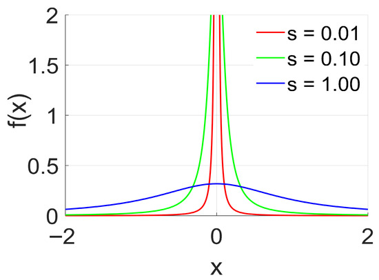
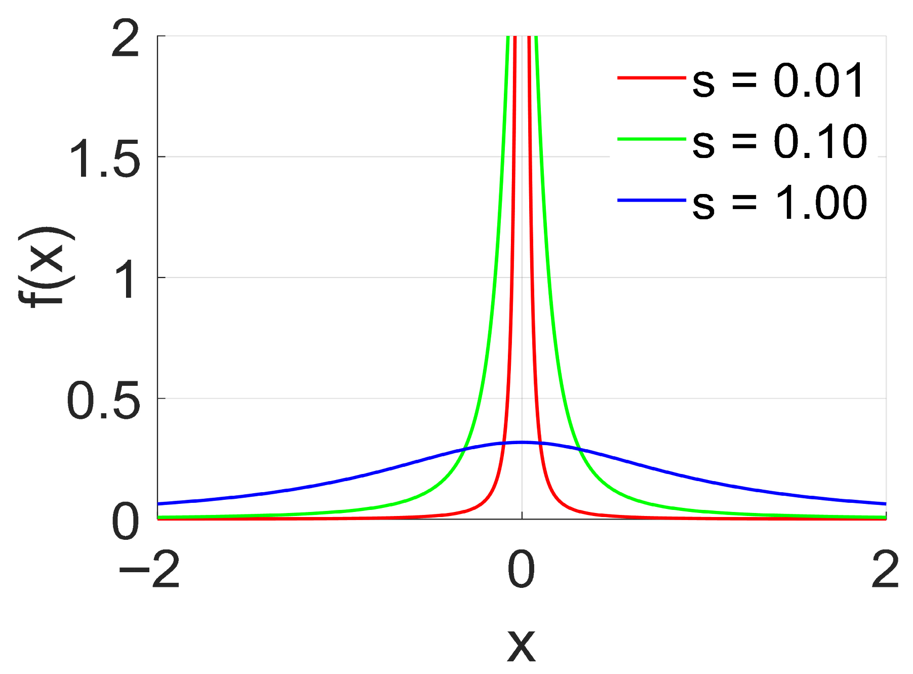
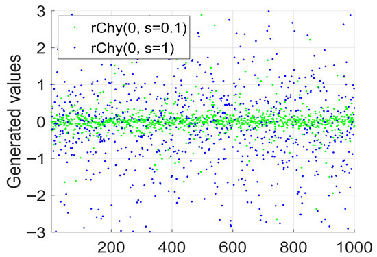
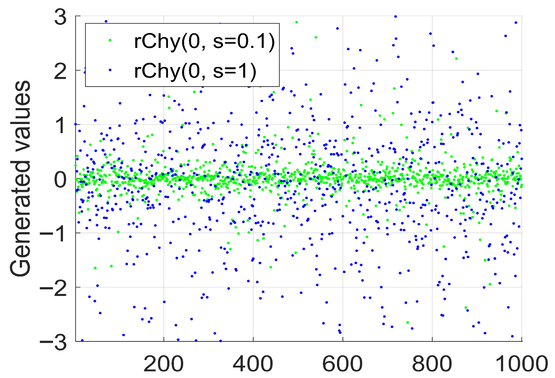
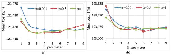
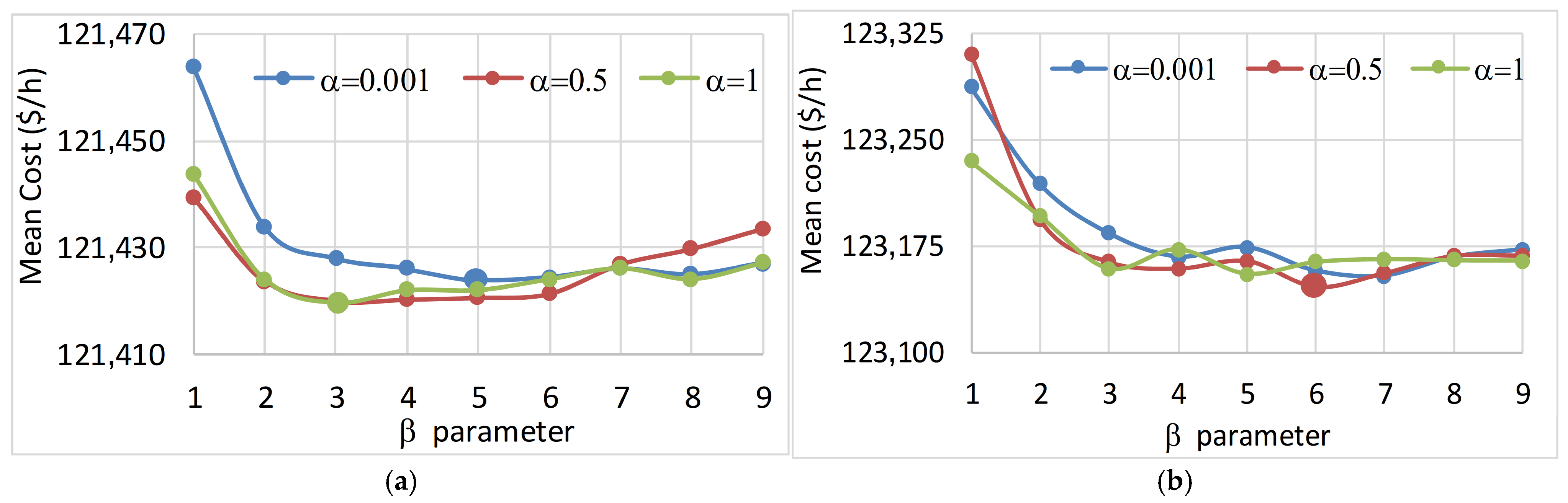
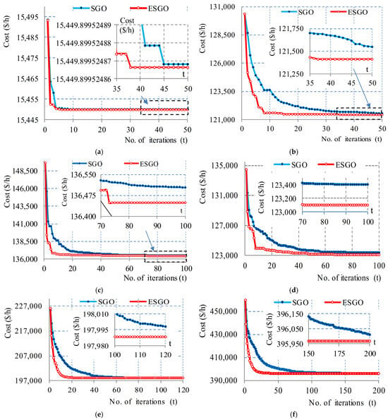
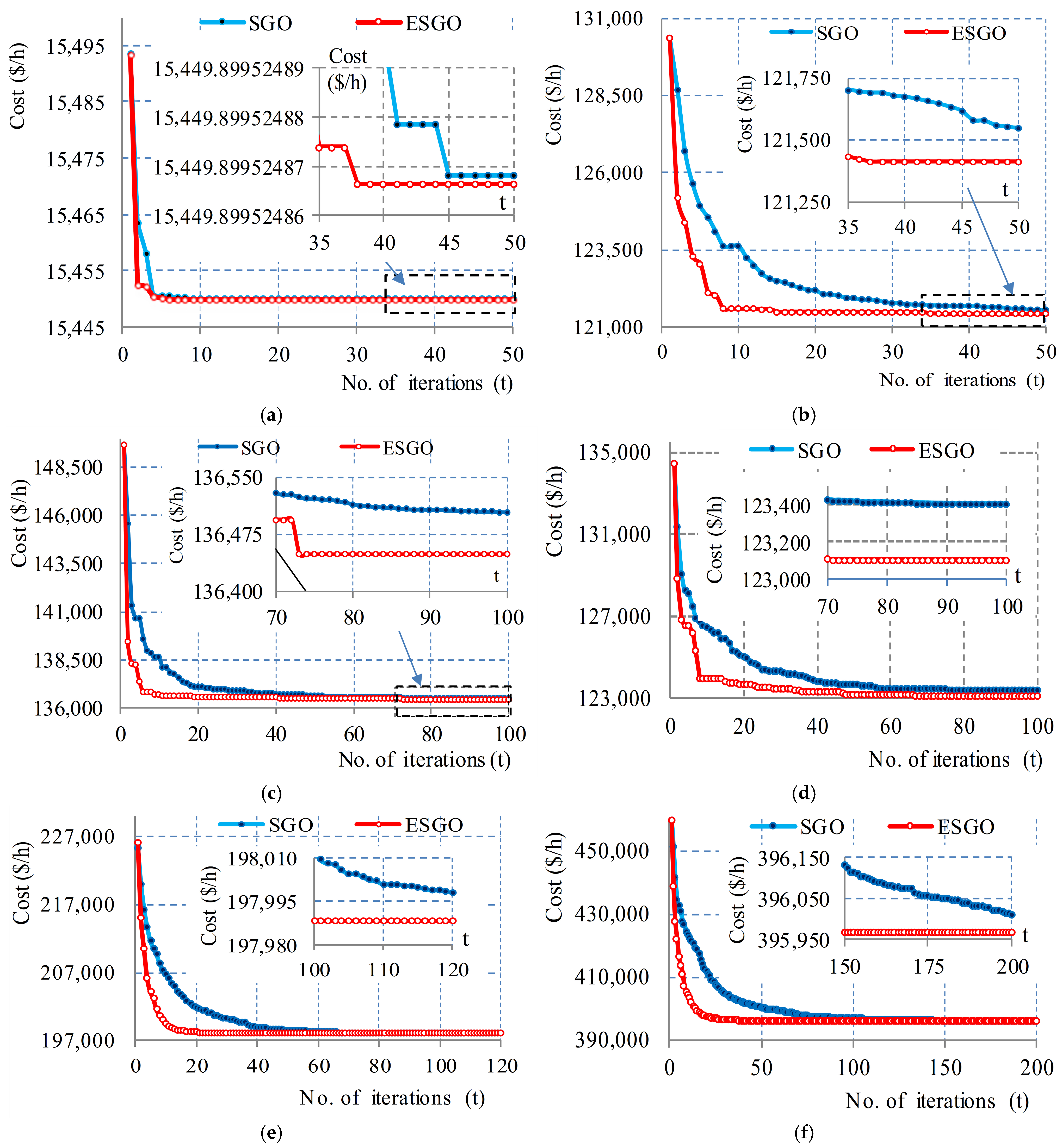
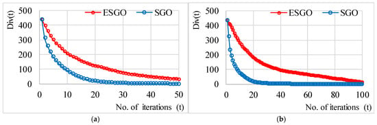
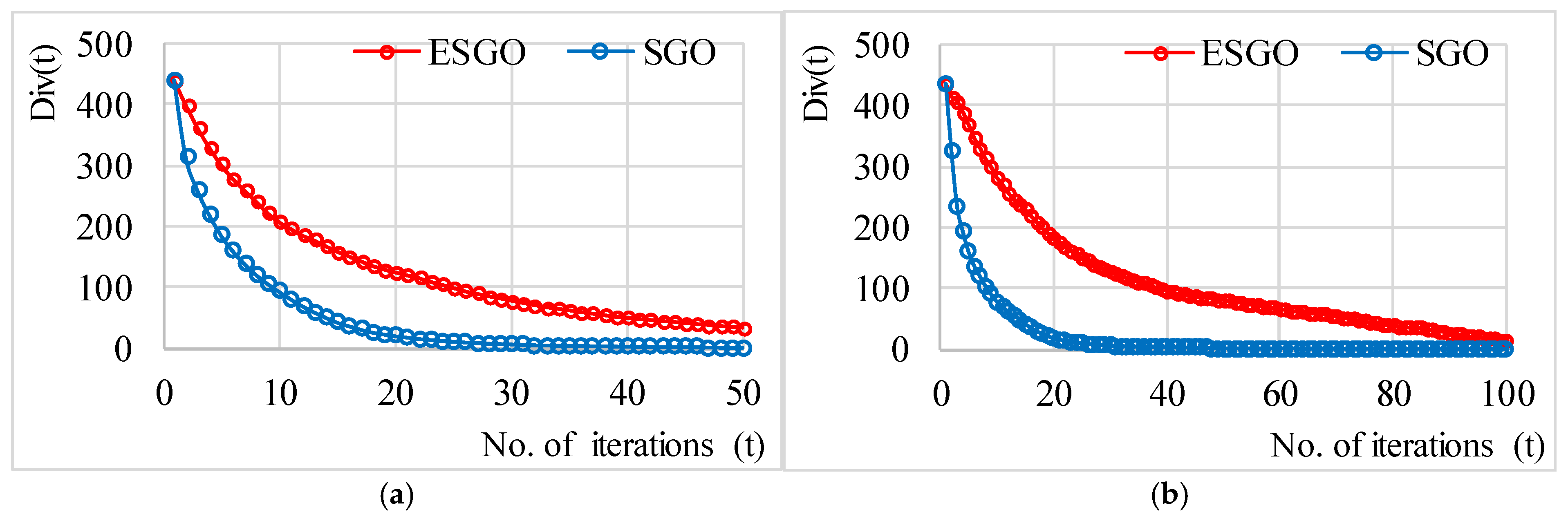
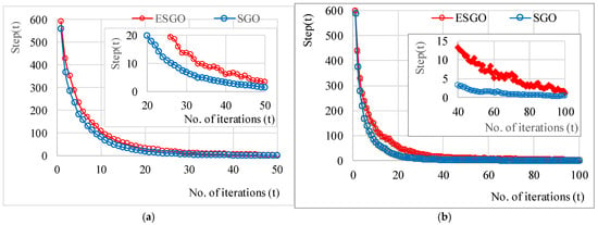
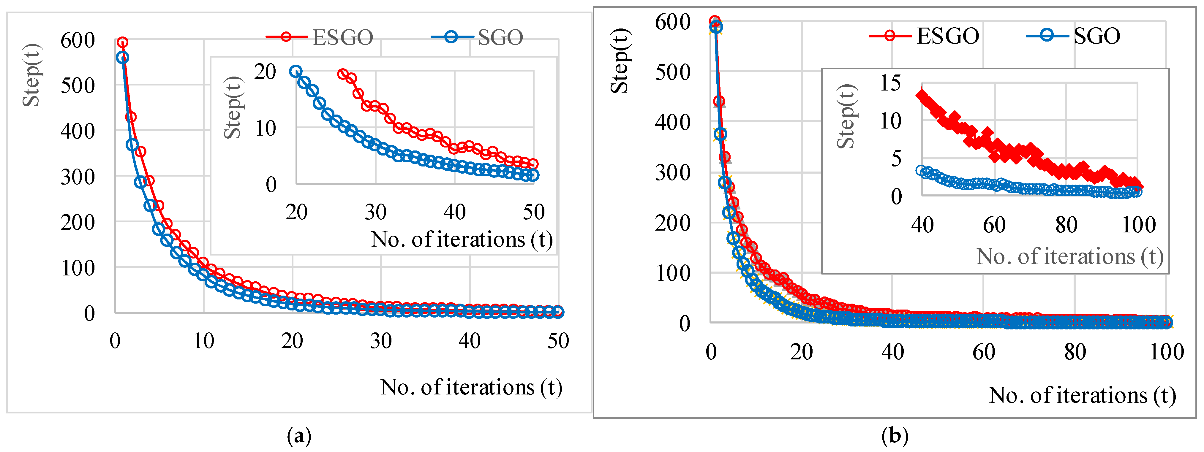

Disclaimer/Publisher’s Note: The statements, opinions and data contained in all publications are solely those of the individual author(s) and contributor(s) and not of MDPI and/or the editor(s). MDPI and/or the editor(s) disclaim responsibility for any injury to people or property resulting from any ideas, methods, instructions or products referred to in the content. |
© 2026 by the authors. Licensee MDPI, Basel, Switzerland. This article is an open access article distributed under the terms and conditions of the Creative Commons Attribution (CC BY) license.