Multi-Dimensional Comfort and EV Stochasticity-Aware Optimization Strategy for Residential PV Storage Systems

Abstract

Residential photovoltaic–battery energy storage systems (PV-BESSs) and electric vehicles (EVs) expose households to a persistent conflict between electricity cost minimization and multi-dimensional comfort. This paper proposes a day-ahead joint scheduling strategy for a PV-BESS, flexible household loads, and a vehicle-to-grid (V2G) capable EV that explicitly quantifies this trade-off. Thermal comfort and temporal preference satisfaction are formulated as bounded indicators and aggregated into a single electricity-consumption comfort index through the efficacy coefficient method. EV availability is characterized by a probability-distribution-based travel model, in which Monte Carlo sampling of the daily mileage and return time is decoupled offline from the optimization so that the conditional charging and discharging logic reduces to linear constraints, and a two-stage scenario-based extension with a chance constraint on the departure energy requirement co-optimizes the household schedule against travel uncertainty. The economic and comfort objectives, explicitly incorporating a cycle-based battery degradation cost to accurately evaluate V2G arbitrage profitability, are combined by a normalized weighted-sum scalarization, and the resulting mixed-integer program with convex quadratic comfort constraints is solved to proven global optimality by GUROBI through YALMIP. For a typical summer household in Southern China, the proposed strategy reduces the daily electricity cost by approximately 7.3% (from 10.69 CNY to 9.91 CNY) at the price of a moderate decrease in the comfort index from 0.86 to 0.77. A sensitivity study of the peak–valley penalty coefficient further shows that flattening the load profile by 1.5 kW raises the user’s daily cost by 2.4 CNY, quantifying the compensation a distribution utility would need to offer to elicit load smoothing. To account for the inevitable forecasting errors of PV generation and outdoor temperature without incurring prohibitive computational burdens, conservative reserve margins and adaptive thermal bounds are introduced into the formulation. Relative to the deterministic representative-scenario schedule, the stochastic extension reduces the expected out-of-sample cost while raising the probability of meeting the EV departure energy requirement from 91.4% to 98.3%. Furthermore, comprehensive benchmark comparisons against pure cost minimization, pure comfort maximization, and deterministic schedules reveal the superiority of the proposed multi-dimensional index over conventional one-dimensional penalties in balancing household economics and occupant satisfaction.

1. Introduction

In recent years, the shortage of conventional energy has become increasingly severe, whereas PV generation offers distinct advantages such as cleanliness and renewability. Consequently, the development of renewable energy has become an essential component of national energy strategies, as supported by the adaptive control studies of hybrid energy storage [1] and the optimization of solar collector models [2]. Currently, the double-sided uncertainty of both generation and load sides constitutes a core challenge for power system scheduling [3]. To address the limitations of conventional energy sources, PV-BESSs utilize PV modules to convert solar energy into electricity and store it, thereby improving the PV utilization efficiency and providing an effective path for energy conservation. The viability of this path has been verified through economic analyses of PV stations [4] and empirical emission-benefit studies of distributed energy systems [5].

A HEMS schedules household loads by analyzing system information such as load profiles, energy storage status, and electricity tariffs [6]. Spanning the critical sectors of smart homes, EVs, and renewable energy, the HEMS has emerged as a pivotal hub for enhancing residential energy efficiency and alleviating grid pressure [7], and comprehensive reviews of HEMS modeling approaches and their computational complexity are provided by Beaudin and Zareipour [8]. Early HEMS formulations focused primarily on cost minimization, which often overlooks dynamic pricing impacts and complex customer behaviors. For instance, Jin et al. [9] highlighted the necessity of considering user comfort in wind power accommodation, while Shafie-Khah and Siano [10] emphasized the impact of response fatigue in stochastic environments. This conventional approach shows clear limitations in accommodating personalized electricity-use habits. Consequently, electricity consumption comfort has been introduced into HEMS optimization as a core metric for multi-objective coordination. Paterakis et al. [11] scheduled household appliances under day-ahead pricing and load-shaping demand response while respecting user-defined operating preferences, and Mohsenian-Rad and Leon-Garcia [12] formulated optimal residential load control that balances the electricity payment against the waiting discomfort induced by load shifting. Recently, Zaytoun et al. [13] developed a robust multi-objective HEMS optimization model that incorporates realistic load classification to comprehensively address user discomfort alongside multi-source uncertainties, and a broad survey of comfort-aware demand response within the HEMS is given by Shareef et al. [14]. For residential flexible loads, accurate quantification of thermal constraints in thermostatically controlled appliances is essential to balance grid demand and occupant preferences. This concept has been explored through the multi-timescale demand response modeling by Liu et al. [15] and the coordinated EV storage scheduling strategy proposed by Yao et al. [16].

As flexible mobile storage, EVs facilitate renewable integration and economic system operation through the joint scheduling of charging and discharging behaviors with renewable outputs. Recent research has systematically evaluated the design challenges and viability of advanced residential EV charging infrastructures [17], and its impacts on distribution systems were reviewed by Yilmaz and Krein [18]. Yang et al. [19] examined residential scheduling with renewable energy and battery storage, Roh and Lee [20] verified the economic benefits of bidirectional flexible-load utilization, while recent studies have further demonstrated the efficacy of practical HVAC operational adjustments in balancing thermal comfort and energy efficiency [21]. However, integrating EVs as mobile storage introduces significant temporal uncertainty. Specifically, Zhou and Sun [22] evaluated the impact of vehicle-to-grid interactions within microgrids, Kanakadhurga and Prabaharan [23] demonstrated the necessity of handling EV uncertainty in smart home demand response, and Cheng et al. [24] highlighted the challenge of travel demand randomness in multi-timescale management. Furthermore, for large-scale EV charging and discharging, single-objective scheduling can no longer meet practical needs, and coordinated frameworks that integrate user cost reduction with grid load-variance mitigation are required [25]; the joint scheduling of EV V2G capability with stationary household storage has been shown to enhance flexibility and economic efficiency in the demand response phase [26]. In parallel, recent studies on prosumer operation planning in retail electricity markets [27] highlight the need to align household-level scheduling with market-side incentive design.

Synthesizing the above literature, three limitations remain. First, studies that incorporate user comfort into the HEMS generally treat the EV connection period as deterministic, so the coupling between EV travel stochasticity and household comfort is not captured. Second, studies that address EV uncertainty typically optimize a single economic objective and quantify comfort, if at all, through one-dimensional penalty terms rather than a bounded multi-dimensional index. Third, joint PV-BESS-EV scheduling frameworks, as explored in the hierarchical dispatch model by Hou et al. [26], the joint optimization methods in [28], and the recent robust integration of PV, EV charging, and demand response by Karimianfard [29], rarely embed an explicit load-smoothing compensation mechanism, In essence, the current literature lacks a unified optimization framework that concurrently incorporates EV travel stochasticity, a multi-dimensional dynamic comfort index, and an explicit mechanism to quantify the economic value of load smoothing. To fill this gap, this paper integrates a probability-distribution-based EV travel model with a multi-dimensional dynamic comfort index within a single day-ahead scheduling framework and quantifies the resulting cost–comfort–smoothness trade-offs, translating the trade-off frontier into an explicit compensation price signal, expressed in CNY per kW of peak–valley reduction, for demand response program design. The main contributions of this paper are summarized as follows:

(1) A bounded multi-dimensional electricity-consumption comfort index is constructed. Thermal comfort and temporal preference satisfaction are each normalized to the interval [0, 1] and aggregated through the efficacy coefficient method so that the comfort degradation caused by load shifting and by temperature relaxation is measured on a single interpretable scale.

(2) A probability-distribution-based EV availability model is developed and made solver-compatible. Monte Carlo sampling of the daily mileage and return time is decoupled offline from the optimization so that the conditional EV charging and discharging logic reduces to linear constraints on binary state variables; the overall scheduling problem is a mixed-integer program whose only nonlinearities are convex quadratic comfort constraints, and it is solved to proven global optimality. A two-stage scenario-based extension with a chance constraint on the departure energy requirement further immunizes the first-stage household schedule against travel uncertainty.

(3) The trade-off frontier between the grid-side peak–valley penalty mechanism and the user’s operating cost is quantified over a range of penalty coefficients, providing a concrete data reference for designing dynamic pricing and demand response compensation mechanisms.

The remainder of this paper is organized as follows: Section 2 describes the physical and decision layer frameworks of the proposed HEMS. Section 3 models the flexible and schedulable household loads. Section 4 formulates the Mixed-Integer Quadratically Constrained Programming (MIQCP) model, detailing the comfort indicators and stochastic extensions. Case studies and numerical analyses under varying penalty coefficients and travel parameters are conducted in Section 5. Finally, Section 6 concludes the paper.

2. HEMS Structure Analysis

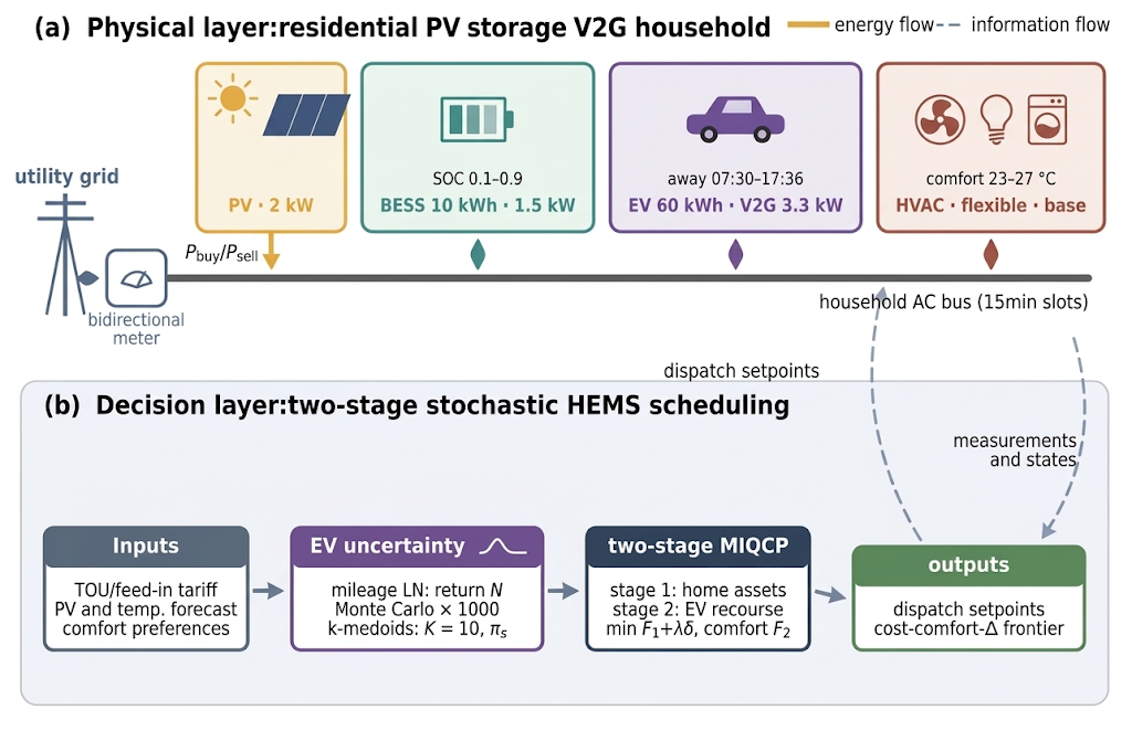
The HEMS is based on smart grid and smart home technology platforms, comprehensively integrating multiple factors such as natural conditions, time-of-use (TOU) electricity tariffs, and consumer power consumption habits. According to their operational characteristics, household loads are classified into three distinct categories: baseloads (or critical loads), such as refrigerators and lighting devices, which exhibit fixed electricity demands and are generally non-adjustable; schedulable loads (or deferrable loads), such as washing machines and dishwashers, whose start and stop times can be intelligently scheduled by the HEMS based on information like TOU electricity tariffs; and thermostatically controlled loads (TCLs), such as air conditioners, the operation of which must balance energy efficiency with the user’s thermal comfort range. The schematic structure of the proposed HEMS is illustrated in Figure 1. The system encompasses two main layers. In the physical layer (Figure 1a), the rooftop PV, the BESS, the V2G-capable EV, and the household loads are coupled to the utility grid through the household AC bus and a bidirectional meter. In the decision layer (Figure 1b), exogenous inputs (such as tariffs, forecasts, and comfort preferences) alongside the EV travel-uncertainty model (which utilizes Monte Carlo sampling followed by k-medoids reduction to K = 10 scenarios) feed the two-stage MIQCP model. The first stage of this optimization commits the home assets, while the second stage adapts the EV schedule according to each scenario. Ultimately, the resulting 15 min dispatch set points and the cost–comfort–Δ trade-off frontier close the loop with the physical layer.

2.1. PV-BESS Model

2.1.1. Photovoltaic System Model

The output power of a residential PV panel depends on the solar radiation intensity, the area of the PV panel, and the photoelectric conversion efficiency [28]. It can be expressed as:

P_PV(t) = A_PVσ_PVG_t

(1)

where P_PV(t) represents the output power of the PV equipment at time t (kW); A_PV denotes the area of the PV solar panel (m²); σ_PV is the photoelectric conversion efficiency; and G_t represents the predicted solar radiation intensity during time interval t (kW/m²).

2.1.2. Battery Energy Storage Model

In practical physical layer implementations, traditional Coulomb counting methods for state-of-charge (SOC) estimation are overly simplistic and highly susceptible to cumulative sensor measurement errors [30]. To ensure the reliable execution of the day-ahead scheduling decisions, the proposed HEMS relies on the underlying Battery Management System (BMS) to perform accurate real-time state monitoring. Therefore, it is assumed that the physical BMS utilizes advanced robust estimation methods, such as Equivalent Circuit Model (ECM)-based algorithms [31], to mitigate sensor inaccuracies and provide high-fidelity initial SOC parameters and operational bounds to the upper-level HEMS optimization framework. This hierarchical decoupling ensures that the exact solvability of the mixed-integer programming at the macro-scheduling level is maintained while preserving robustness against hardware-level measurement noise.

Residential users can store the surplus electricity generated by distributed power sources (such as PV generation) and release it when needed. This achieves autonomous power regulation, thereby improving self-generation utilization and reducing electricity costs. The energy storage model is utilized to represent the variation of the SOC during the charging and discharging processes [29]:

$$\mathit{SOC}(t+1)=\left\{\begin{array}{l}\mathit{SOC}(t)+{\displaystyle \frac{{\eta }_c{P}_{\mathit{bat},\mathit{ch}}(t)\Delta t}{C_{\mathit{bat}}}}\\ \mathit{SOC}(t)-{\displaystyle \frac{P_{\mathit{bat},\mathit{dis}}(t)\Delta t}{{\eta }_d{C}_{\mathit{bat}}}}\end{array}\right.$$

(2)

SOC_min ≤ SOC(t) ≤ SOC_max

(3)

where SOC represents the state of charge of the battery energy storage system at time t; P_bat,ch and P_bat,dis denote the charging and discharging power of the battery at time t, respectively (kW); η_c and η_d are the charging and discharging efficiencies of the battery, respectively; and $C_{\mathit{bat}}$ is the total capacity of the battery energy storage system (kWh).

2.2. EV Charging and Discharging Strategy

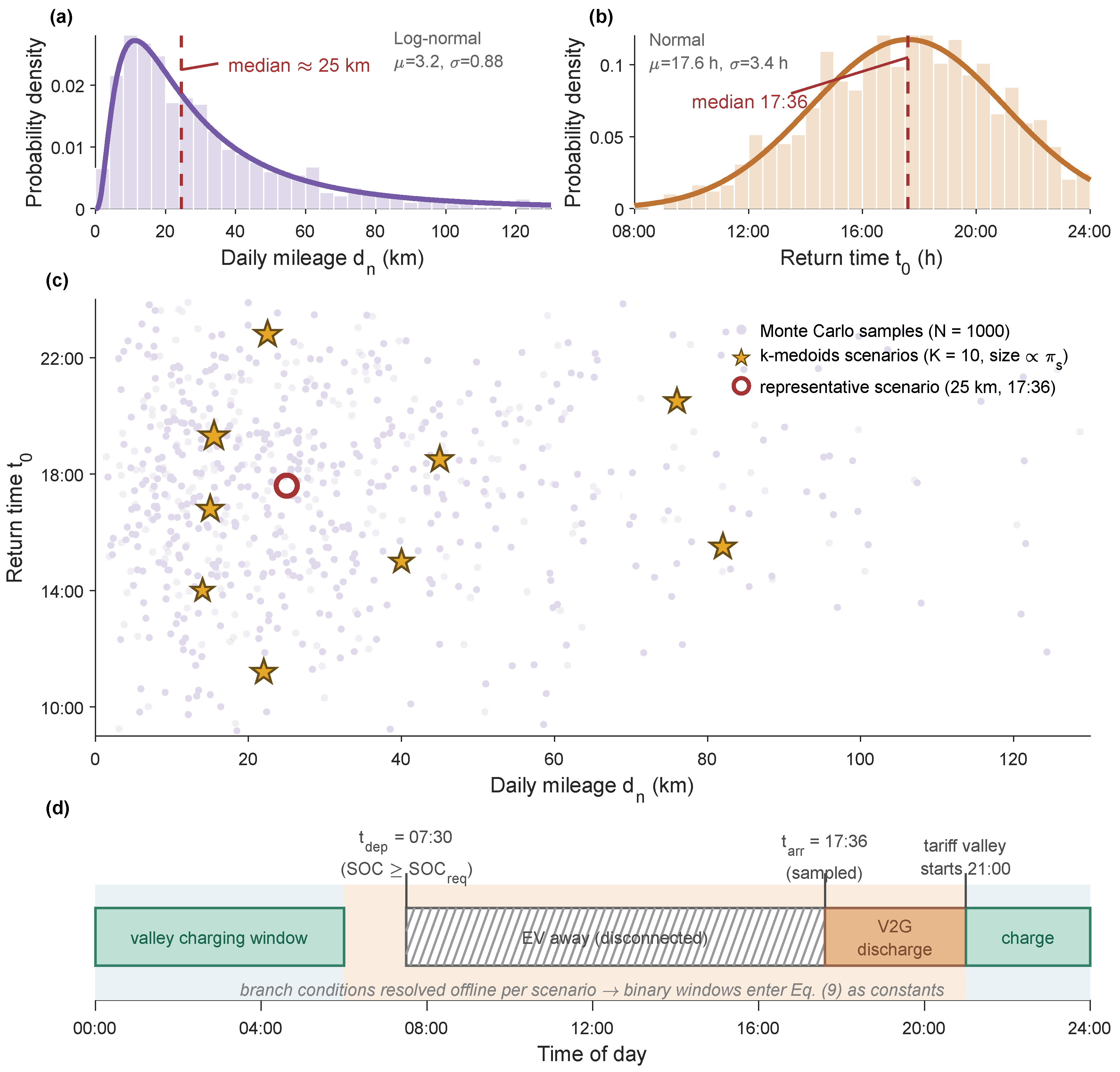
As a mobile energy storage device, an EV can function as both a load and an energy storage unit. Therefore, it is essential to properly schedule the charging and discharging strategy according to the user’s travel habits: charging during electricity tariff troughs and discharging during tariff peaks. Considering the randomness of EV travel, the daily travel mileage is assumed to follow a log-normal distribution, which aligns with recent predictive models of EV charging loads based on user travel characteristics [32]:

$$f_l(x)={\displaystyle \frac{1}{x{\mu }_l\sqrt{2\pi }}}\exp \left[{\displaystyle \frac{{(\ln x-{\mu }_l)}^2}{2{\sigma }_l^2}}\right]$$

(4)

where μ_l = 3.2 and σ_l = 0.88 represent the mean and standard deviation of the travel mileage logarithmic values, respectively.

Assuming that the last charging connection time corresponds to the user’s return time, this arrival time satisfies a normal distribution, which can be expressed as:

$$f_t(x)=\left\{\begin{array}{l}{\displaystyle \frac{1}{{\sigma }_t\sqrt{2\pi }}}\exp \left[-{\displaystyle \frac{{(x+24-{\mu }_t)}^2}{2{\sigma }_t^2}}\right],0<x\le {\mu }_t-12\\ {\displaystyle \frac{1}{{\sigma }_t\sqrt{2\pi }}}\exp \left[-{\displaystyle \frac{{(x-{\mu }_t)}^2}{2{\sigma }_t^2}}\right],{\mu }_t-12<x\le 24\end{array}\right.$$

(5)

where μ_t = 17.6 and σ_t = 3.4 denote the mean and standard deviation of the user’s return time, respectively.

Assuming that the end time of the surplus PV generation period is T_start,p and the start time of the evening peak period is T_start,e, the EV charging start time T_start,c and discharging start time T_start,d are determined by comparing the EV return time t₀(i) with the surplus PV generation period and the evening peak period. When t₀(i) ≤ T_start,p, the charging start time is set as the return time, i.e., T_start,c = t₀(i). Conversely, when T_start,p ≤ t₀(i) ≤ T_start,e, the discharging start time corresponds to the start time of the evening peak, i.e., T_start,d = T_start,e. When t₀(i) ≥ T_start,e, the discharging start time is defined as the user’s return time, i.e., T_start,d = t₀(i).

Simultaneously, the EV charging and discharging strategy proposed in this paper complies with the following two prerequisites: it must neither exceed the maximum depth of discharge (DOD) of the EV battery nor compromise the user’s daily travel demands. To this end, the maximum discharge capacity of the EV should be the minimum value allowed by both constraints, which can be formulated as [33,34]:

$$C_{\mathit{dischar}}(i)=\min \left\{(S_{\mathit{EV}}^{\max }-S_{\mathit{EV}}^{\min })E_{\mathit{EV}}-L(i)\omega ,\delta E_{\mathit{EV}}\right\}$$

(6)

where $S_{\mathit{EV}}^{\max }$ and $S_{\mathit{EV}}^{\min }$ represent the upper and lower limits of the EV SOC, respectively; E_EV denotes the total capacity of the EV battery; L(i) is the driving distance of the i-th vehicle; ω represents the energy consumption rate per kilometer of the EV; and δ denotes the maximum allowable depth of discharge (DOD).

During the grid-connected period, the EV state of charge evolves analogously to that of the stationary battery, and the state of charge at the plug-in (arrival) time is determined by the sampled daily mileage:

$$\begin{array}{l}\mathit{SO}{C}_{\mathit{EV}}(t+1)=\mathit{SO}{C}_{\mathit{EV}}(t)+[{\eta }_{\mathit{ch}}{P}_{\mathit{EV},\mathit{ch}}(t)-P_{\mathit{EV},\mathit{dis}}(t)/{\eta }_{\mathit{dis}}]\Delta t/E_{\mathit{EV}},\\ t\in [t_{\mathit{arr}},t_{\mathit{dep}}]\end{array}$$

(7)

$$\mathit{SO}{C}_{\mathit{EV}}(t_{\mathit{arr}})=\mathit{SO}{C}_{\mathit{dep}}-{\displaystyle \frac{d_n\omega }{E_{\mathit{EV}}}}$$

(8)

where SOC_EV(t) is the EV state of charge at time t; P_EV,ch(t) and P_EV,dis(t) are the EV charging and discharging powers (kW); η_ch and η_dis are the corresponding efficiencies; t_arr and t_dep denote the arrival time and the next-day departure time; and SOC_dep is the state of charge at the preceding departure. Outside the interval [t_arr, t_dep], the EV is disconnected from the household and both powers are zero.

The EV charging and discharging strategy illustrated in Figure 2 involves Monte Carlo random sampling and conditional sequential logic, which cannot be embedded directly in a mathematical program. A parameter offline decoupling approach is therefore adopted. First, the daily mileage and return time are sampled offline from Equations (4) and (5) using 1000 Monte Carlo samples with a fixed random seed; the branch conditions in Figure 2, which compare the sampled return time with the end of the PV surplus period and the start of the evening peak, are evaluated at this stage so that the charging start time, the discharging start time, and the next-day departure time enter the optimization as known constants of the selected scenario. Second, given these constants, the admissible charging and discharging periods are imposed on the binary state variables through the linear equalities and the mutual-exclusion inequality of Equation (9), and the binaries are coupled to the continuous charging and discharging powers only through the box constraints presented in Section 4.3. Because every conditional branch is resolved before optimization, no big-M constants are required, and the EV control logic contributes only linear constraints to the scheduling model.

$$\left\{\begin{array}{l}{u}_{\mathit{ch}}(t)+u_{\mathit{dis}}(t)\le 1,\forall t\in [1,n]\\ u_{\mathit{ch}}(t)=0,u_{\mathit{dis}}(t)=0,\forall t\notin [t_0(i),t_{\mathit{dep}}(i)]\end{array}\right.$$

(9)

Here, u_ch(t) and u_dis(t) represent the binary charging and discharging states of the EV at time t, respectively; t_dep(i) denotes the departure time of the EV on the following day; and n represents the total number of time slots within the scheduling horizon.

3. Household Load Modeling

According to the operational characteristics of household electricity loads, they can be classified into two major categories: baseloads and flexible loads. Baseloads refer to the types of electricity consumption characterized by fixed operational demands, non-adjustability, and a lack of scheduling capability, such as lighting and televisions. In contrast, flexible loads can be further subdivided into two categories: (1) schedulable loads, such as dishwashers and washing machines (these loads possess a certain degree of adjustability regarding their startup times, but their operation cannot be interrupted once initiated), and (2) HVAC equipment, such as air conditioners, whose operational states are governed by temperature settings (their operation can be interrupted during the process, but their overall operating time windows are non-shiftable).

The fundamental operational principle of the HEMS is ‘self-consumption and grid-feeding’. By shifting flexible loads from high-tariff periods to low-tariff periods or from periods with low PV outputs to periods with high PV outputs, the household energy efficiency can be effectively enhanced and the energy consumption cost optimized [35].

3.1. HVAC Load

The load of a single air conditioning unit is formulated utilizing a discrete equivalent thermal parameter (ETP) model, obtained as the exact one-slot solution of the first-order building heat-balance equation [36]:

T_in(t + 1) = e^−Δt/RCT_in(t) + R(e^−Δt/RC − 1)P_hvac(t) + (1 − e^−Δt/RC)T_out(t)

(10)

where T_in and T_out represent the indoor and outdoor temperatures at time t, respectively (°C); R denotes the thermal resistance of the room (°C/kW); C represents the thermal capacity of the room (kWh/°C); and P_hvac is the electrical power of the air conditioner (kW).

3.2. Schedulable Load

Schedulable loads can be summarized by the following typical characteristics: they exhibit a continuous working mode within a single operational cycle, their operating power remains approximately constant during this period, and they possess a predefined fixed working duration. The operating time windows of such loads can be shifted as a whole within the scheduling horizon. However, their startup and shutdown schedules must simultaneously satisfy the total operational duration constraint as well as the predefined allowable startup time window constraint. Taking a dishwasher as an example, the schedulable load model is constructed as follows:

$$t_{\mathit{wash}}^{\mathit{end}}=t_{\mathit{wash}}^{\mathit{start}}+T_{\mathit{wash}}^{\mathit{set}}$$

(11)

$$G_{\mathit{wash},i}(t)=\left\{\begin{array}{l}1,t\in [t_{\mathit{wash}}^{\mathit{start}},t_{\mathit{wash}}^{\mathit{end}}]\\ 0,t\notin [t_{\mathit{wash}}^{\mathit{start}},t_{\mathit{wash}}^{\mathit{end}}]\end{array}\right.$$

(12)

where $t_{\mathit{wash}}^{\mathit{start}}$ and $t_{\mathit{wash}}^{\mathit{end}}$ represent the start and end time slots of the dishwasher’s operation, respectively; $T_{\mathit{wash}}^{\mathit{set}}$ denotes the number of continuous operational time slots required; and G_wash,i(t) indicates the operational status of the dishwasher at time t.

4. Optimization Model Formulation

4.1. Multi-Dimensional Comfort Indicators

4.1.1. Thermal Comfort Indicator

The thermal comfort indicator is constructed from the normalized deviation of the indoor temperature from the user’s preferred set point. Deviations are measured relative to the widths of the acceptable band on either side of the set point, so that the instantaneous indicator equals 1 when the indoor temperature coincides with the set point, decreases quadratically as the temperature approaches either band limit, and reaches 0 at the limits; the quadratic form penalizes large deviations progressively more strongly than small ones, consistent with the nonlinear sensitivity of perceived thermal comfort [36]. The thermal comfort indicator function is formulated as follows:

$$\left\{\begin{array}{l}\mathit{TC}={\displaystyle \frac{{\displaystyle \sum _{t=1}^n\frac{e^{L_{\mathit{AC}}(t)}-1}{e-1}{g}_{\mathit{AC}}(t)}}{{\displaystyle \sum _{t=1}^n{g}_{\mathit{AC}}(t)}}}\\ L_{\mathit{AC}}(t)={\displaystyle \frac{2\times \left|T_{\mathit{in}}(t)-T_{\mathit{set}}(t)\right|}{T_{\mathit{set},\max }-T_{\mathit{set},\min }}}\end{array}\right.$$

(13)

where L_AC(t) represents the percentage deviation between the indoor temperature and the most comfortable temperature set by the user at time t; g_AC(t) denotes the operational state of the air conditioner, taking a value of 0 or 1; T_set(t) is the optimal comfortable indoor temperature set by the user; and T_set,max and T_set,min represent the upper and lower limits of the comfortable temperature range, respectively.

Because the indoor temperature is constrained to remain within the acceptable band whenever the air conditioner is scheduled to operate, each instantaneous term of Equation (13) is bounded in [0, 1]. The quadratic deviation is a convex function of the indoor temperature, which is itself an affine function of the air-conditioning power through Equation (10). The conditional two-branch form of Equation (13) and its product with the binary operating state are handled exactly by decomposing the temperature deviation into non-negative normalized components and introducing an epigraph variable z(t):

$$\left\{\begin{array}{l}{T}_{\mathit{in}}(t)-T_{\mathit{set}}=(T_{\max }-T_{\mathit{set}}){\delta }^{+}(t)-(T_{\mathit{set}}-T_{\min }){\delta }^{-}(t)\\ 0\le {\delta }^{+}(t)\le 1,0\le {\delta }^{-}(t)\le 1\end{array}\right.$$

(14)

$$z(t)+{[{\delta }^{+}(t)]}^2+{[{\delta }^{-}(t)]}^2\le 1$$

(15)

To preserve the convex structure required by the MIQCP solver, the thermal comfort indicator is directly mapped to the quadratic non-negative deviation components. At the optimum, at most one of δ⁺(t) and δ⁻(t) is nonzero, and the epigraph variable z(t) bounds the instantaneous comfort objective.

4.1.2. Temporal Comfort Indicator

Regarding the temporal comfort indicator, the objective is to keep appliance schedules aligned with the user’s habitual electricity-use pattern. For each schedulable load, the user specifies a preferred operating window; the indicator in Equation (16) measures the fraction of each load’s required operating slots that fall inside its preferred window, averaged over all schedulable loads, following the habit-preservation formulation of [37]. The indicator therefore lies in [0, 1], equals 1 when every load runs entirely within its preferred window, and decreases in proportion to the operating time displaced outside that window:

$$\mathit{FC}={\displaystyle \frac{1}{K}}{\displaystyle \sum _{i=1}^K\frac{{\displaystyle \sum _{t=1}^n{G}_{\mathit{wash},i}(t)W_i^{\mathit{pref}}(t)\Delta t}}{T_i^F}}$$

(16)

where K represents the total number of schedulable household loads, and $T_i^F$ denotes the required operational duration of the i-th schedulable load. G_wash,i(t) indicates the operational status of the load at time t, and $W_i^{\mathit{pref}}(t)$ is a binary parameter that equals 1 if time slot t falls within the user’s preferred operating window for appliance i and 0 otherwise. This formulation strictly penalizes operations displaced outside the preferred window.

4.2. Objective Functions and Multi-Objective Scalarization

(1)

Economic Objective Function

The traditional electricity consumption cost C_H is expressed as follows:

$$C_H={\displaystyle \sum _{t=1}^n(r_t{P}_{\mathit{grid}}(t)\frac{24}{n})}$$

(17)

where C_H represents the household electricity cost; n denotes the total number of operational time slots; r_t is the purchasing or selling electricity tariff at time t; and P_grid(t) represents the net power exchanged between the household and the utility grid at time t (kW). When P_grid(t) > 0, the household purchases power from the grid; conversely, when P_grid(t) < 0, the household feeds surplus power back into the grid.

Equation (17) is a compact expression in terms of the net exchange power. Because the purchase tariff and the feed-in remuneration differ, surplus PV power exported to the grid is compensated through a feed-in tariff rather than net metering, and the cost term is implemented with the import and export explicitly separated:

$$\left\{\begin{array}{l}{P}_{\mathit{grid}}(t)=P_{\mathit{buy}}(t)-P_{\mathit{sell}}(t),\\ 0\le P_{\mathit{buy}}(t)\le s_{\mathit{grid}}{P}_{\mathit{grid}}^{\max },\\ 0\le P_{\mathit{sell}}(t)\le [1-s_{\mathit{grid}}{P}_{\mathit{grid}}^{\max }]P_{\mathit{grid}}^{\max }\end{array}\right.$$

(18)

$$\left\{\begin{array}{l}{C}_1={\displaystyle \sum _{t=1}^T[c_{\mathit{buy}}(t)P_{\mathit{buy}}(t)-c_{\mathit{FIT}}{P}_{\mathit{sell}}(t)]\Delta t}+C_{\mathrm{deg}}^{\mathit{BESS}}+C_{\mathrm{deg}}^{\mathit{EV}}\\ C_{\mathrm{deg}}^{\mathit{BESS}}=C_{\mathit{wear}}^{\mathit{BESS}}{\displaystyle \sum _{t=1}^T[P_{\mathit{bat},\mathit{ch}}(t)+P_{\mathit{bat},\mathit{dis}}(t)]\Delta t}\\ C_{\mathrm{deg}}^{\mathit{EV}}=C_{\mathit{wear}}^{\mathit{EV}}{\displaystyle \sum _{t=1}^T[P_{\mathit{EV},\mathit{ch}}(t)+P_{\mathit{EV},\mathit{dis}}(t)]\Delta t}\end{array}\right.$$

(19)

where c_buy(t) and c_FIT are TOU purchasing price and feed-in tariff at time slot t, respectively. $C_{\mathrm{deg}}^{\mathit{BESS}}$ and $C_{\mathrm{deg}}^{\mathit{EV}}$ represent the linearized wear-and-tear costs for the stationary BESS and the EV battery, respectively, which are proportional to their energy throughput: the unit wear costs $C_{\mathit{wear}}^{\mathit{BESS}}$ and $C_{\mathrm{deg}}^{\mathit{EV}}$ (CNY/kWh) are derived from the battery replacement cost apportioned over its total cycle-life energy capacity. Incorporating these terms restrains the optimizer from performing excessive charge–discharge cycles solely for marginal price spreads.

Furthermore, power grids generally expect the user’s load curve to be as smooth as possible. To this end, compensation or incentive mechanisms are often implemented to encourage users to actively adjust their electricity consumption behaviors, thereby optimizing the shape of the load curve. Based on this consideration, the peak–valley difference of the load curve is converted into a corresponding peak–valley difference cost C_PtoV through a coefficient ρ to quantitatively evaluate its economic impact on home energy management:

$$C_{\mathit{PtoV}}=\rho [\underset{t}{\max }(P_{\mathit{grid}}(t))\Delta t-\underset{t}{\min }(P_{\mathit{grid}}(t))\Delta t]$$

(20)

The max and min operators render the peak–valley term nonsmooth; they are removed exactly by introducing auxiliary variables that bound the net exchange power from above and below. Because the peak–valley cost is minimized, the auxiliary variables attain the true peak and valley values at the optimum, so the reformulation is exact:

P_pk ≥ P_grid(t), P_vl ≤ P_grid(t), ∀t; C₂ = λ(P_pk − P_vl)

(21)

In summary, the comprehensive economic objective function can be formulated as:

min(C_PtoV + C_H)

(22)

(2)

Electricity-Consumption Comfort Objective Function

To balance the impacts of different objectives on the scheduling results, the efficacy coefficient method is employed for comprehensive evaluation. This method defines an efficacy coefficient ranging within [0, 1] to assess the performance of a specific objective: a value of 1 indicates the optimal effect of the objective, whereas a value of 0 represents the worst. It is utilized to comprehensively measure the overall performance of the scheduling scheme:

$$C_2=\sqrt[k]{{\displaystyle \prod _{i=1}^k(1-\frac{e^{\mathit{FC}}-1}{e-1}}})$$

(23)

C₃ = 1 − TC

(24)

where C₂ and C₃ represent the efficacy coefficients of the time comfort indicator FC and the thermal comfort indicator TC, respectively.

In summary, the aggregated electricity-consumption comfort objective function is formulated as follows:

$$\max C=\sqrt{C_2{C}_3}$$

(25)

(3)

Multi-Objective Scalarization

The economic objective is measured in CNY, whereas the comfort objective is dimensionless within [0, 1]. The two objectives are combined through a normalized weighted-sum scalarization:

$$\min F={\omega }_1{F}_1/\left|F_1^b\right|-{\omega }_2{F}_2$$

(26)

where $F_1^b$ is the electricity cost of the unoptimized baseline schedule, used as the normalization reference, and ω₁ and ω₂ are non-negative weights with ω₁ + ω₂ = 1. All results in Section 5 are obtained with ω₁ = 0.6 and ω₂ = 0.4, reflecting a user who prioritizes cost saving without trading comfort away entirely. Alternative points on the Pareto frontier can be generated by varying the weight ratio or by imposing an ε constraint on the comfort objective, and the peak–valley penalty sweep in Section 5.2 illustrates one section of this frontier.

(4)

Scenario-Based Stochastic Extension

The representative-scenario model of Equation (26) quantifies the trade-offs for the median travel pattern, but the household decisions taken before the actual travel realization is known should be robust to travel uncertainty. Following two-stage stochastic HEMS formulations [38,39], the model is therefore extended as follows: The 1000 Monte Carlo samples are reduced to K = 10 representative scenarios with probabilities π_s by k-medoids clustering in the (daily mileage, return time) plane. The schedules of the schedulable loads, the HVAC, and the BESS are first-stage (here-and-now) decisions shared by all scenarios, whereas the EV charging and discharging trajectories are second-stage (wait-and-see) decisions indexed by the scenario s. The expected-cost counterpart of Equation (26) is:

$$\min F={\omega }_1{\displaystyle \sum _{s=1}^K{\pi }_s{C}_{1,s}}/\left|F_1^b\right|-{\omega }_2{F}_2$$

(27)

In addition, the punctual availability of the vehicle is protected by a chance constraint requiring the departure energy requirement of Equation (35) to be met with probability at least 1 − ε, implemented exactly for the finite scenario set through per-scenario binary violation indicators:

$$\mathit{SO}{C}_{\mathit{EV},s}(t_{\mathit{tep}})\ge \mathit{SO}{C}_{\mathit{rep}}-M{\xi }_s,{\displaystyle \sum _{s=1}^K{\pi }_s{\xi }_s\le \epsilon ,{\xi }_s\in \left\{0,1\right\}},\forall s$$

(28)

Here, ξ_s indicates violation of the departure requirement in scenario s, ε = 0.05 is the risk budget, and M = SOC_rep − SOC_min is a tight big-M constant bounded by the SOC range itself. The extension preserves the mixed-integer convex structure of the model; its out-of-sample value relative to the deterministic representative-scenario schedule is quantified in Section 5.4.

4.3. Constraints

The operational logic of the proposed HEMS must strictly satisfy several physical and technical constraints to ensure system security and stability:

(1) Real-time Power Balance Constraint: The instantaneous power equilibrium among household load, PV generation, battery energy storage system (BESS), and the utility grid must be maintained at each time slot.

P_load(t) = P_grid(t) + P_PV(t) + P_bat,dis(t) − P_bat,ch(t) − P_EV,ch(t) + P_EV,dis(t)

(29)

(2) PV Output Constraint: The output power of the PV system is bounded by its rated capacity:

0 ≤ P_PV(t) ≤ P_PV,max

(30)

where P_PV,max represents the rated power capacity of the PV system (kW).

(3) BESS Operational Constraints: The charging and discharging power of the household battery must lie within its maximum limits, accompanied by a binary mutually exclusive state constraint to prevent concurrent charging and discharging actions.

0 ≤ P_bat,ch(t) ≤ u_bat,ch(t)P_batmax

(31)

0 ≤ P_bat,dis(t) ≤ u_bat,dis(t)P_batmax

(32)

u_bat,ch(t) + u_bat,dis(t) ≤ 1, ∀t ∈ [1, n]

(33)

P_batmax denotes the maximum allowable charging and discharging power of the stationary battery (kW); u_bat,dis and u_bat,dis are the binary indicators managing the BESS charging and discharging states at time t, respectively.

In addition, the stored energy must remain within its permissible range at every time slot, and the initial and terminal states of charge are fixed to a common value so that the day-ahead schedule is energy-neutral for the BESS and repeatable across days:

SOC_min ≤ SOC(t) ≤ SOC_max, SOC(0) = SOC(T) = SOC_ini

(34)

where SOC_ini = 0.5 is adopted in the case study. The corresponding terminal condition for the EV is imposed by the departure energy constraint of Equation (35).

(4) EV Departure Energy Constraint: Upon the EV’s departure on the following day, its state of charge must be sufficient to support the driving mileage simulated via Monte Carlo sampling while preserving the predefined minimum battery operating capacity.

$$\mathit{SO}{C}_{\mathit{EV}}(t_{\mathit{dep}})\ge S_{\mathit{EV}}^{\min }+{\displaystyle \frac{L(i)\omega }{E_{\mathit{EV}}}}$$

(35)

SOC_EV(t_dep) is the remaining state of charge of the EV battery at the next day’s departure time t_dep.

(5) EV Interactivity Limits: The interactive charging and discharging power of the EV must strictly comply with its technical upper and lower bounds.

$$0\le P_{\mathit{EV},\mathit{ch}}(t)\le u_{\mathit{ch}}(t)P_{\mathit{EV},\mathit{ch}}^{\max }$$

(36)

$$0\le P_{\mathit{EV},\mathit{dis}}(t)\le u_{\mathit{dis}}(t)P_{\mathit{EV},\mathit{dis}}^{\max }$$

(37)

$P_{\mathit{EV},\mathit{ch}}^{\max }$ and $P_{\mathit{EV},\mathit{dis}}^{\max }$ represent the instantaneous charging and discharging power of the EV at time t, respectively (kW).

4.4. Assumptions and Simplifications

The scheduling model contains binary variables for the load start and stop statuses and for the mutually exclusive charging and discharging states of the BESS and the EV; all constraints are linear except the convex quadratic comfort constraints of Equation (15). To preserve this structure and to ensure that branch-and-bound reaches a certified global optimum within seconds, the following assumptions and simplifications are adopted in this study:

(1) The building’s thermal dynamic model is simplified, wherein the equivalent thermal resistance R and thermal capacitance C are assumed to be constant parameters, ignoring the higher-order nonlinear disturbances caused by complex human activities.

(2) Recent critical analyses on the state-of-health of lithium-ion batteries indicate that the degradation attributable to realistic V2G utilization is small per unit of energy throughput but not negligible [35]; for a lithium iron phosphate pack, a commonly adopted equivalent degradation cost is on the order of 0.05–0.10 CNY per kWh of discharged energy. In the case study of Section 5.3, the EV discharges roughly 15 kWh on a typical day, so accounting for degradation would add approximately 0.8–1.5 CNY per day and would reduce the V2G arbitrage benefit (about 4.5 CNY per day at λ = 0) by roughly 20–35%, without altering the qualitative conclusions. A full cycle-life-aware formulation is left for future work.

4.5. Rationale for Optimization Method Selection

The selection of the optimization algorithm is critical to the performance of the HEMS. Nature-inspired meta-heuristic techniques have demonstrated significant efficacy in handling highly complex, non-convex, and black-box economic evaluations, such as the dispatch of virtual power plants. However, meta-heuristic algorithms (e.g., Particle Swarm Optimization or Genetic Algorithms) typically struggle with strict discrete operational constraints and mutually exclusive logic, often requiring heavy penalty functions that can lead to local optima and extensive computation times.

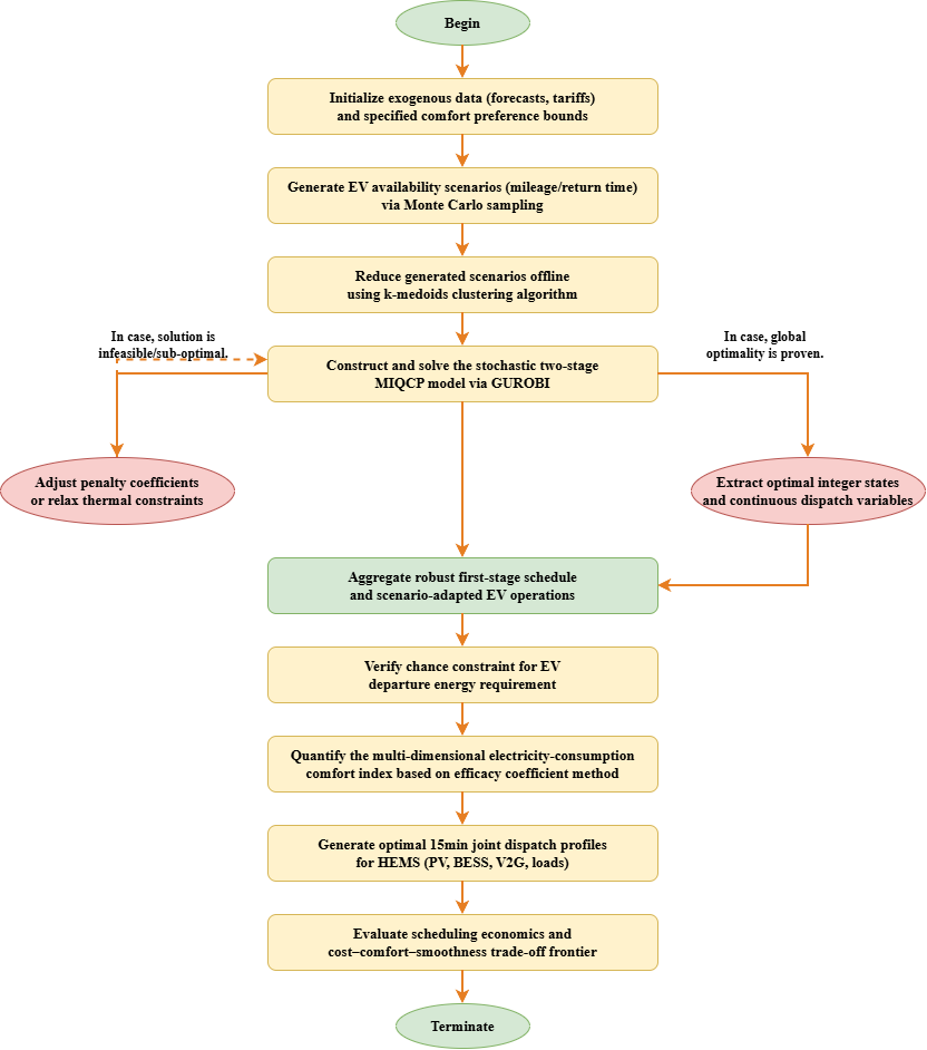
To systematically solve the formulated MIQCP model, the step-by-step optimization logic is detailed in the newly added Algorithm Flowchart (Figure 3). It is worth noting that while multiple nature-inspired meta-heuristic techniques have been recently employed to evaluate the economic viability and perform complex scheduling for broader energy architectures like virtual power plants [40], this study leverages the exact mathematical programming solver GUROBI through YALMIP to guarantee the proven global optimality of the residential HEMS dispatch.

5. Case Study

5.1. Scenario Setup and Parameter Configuration

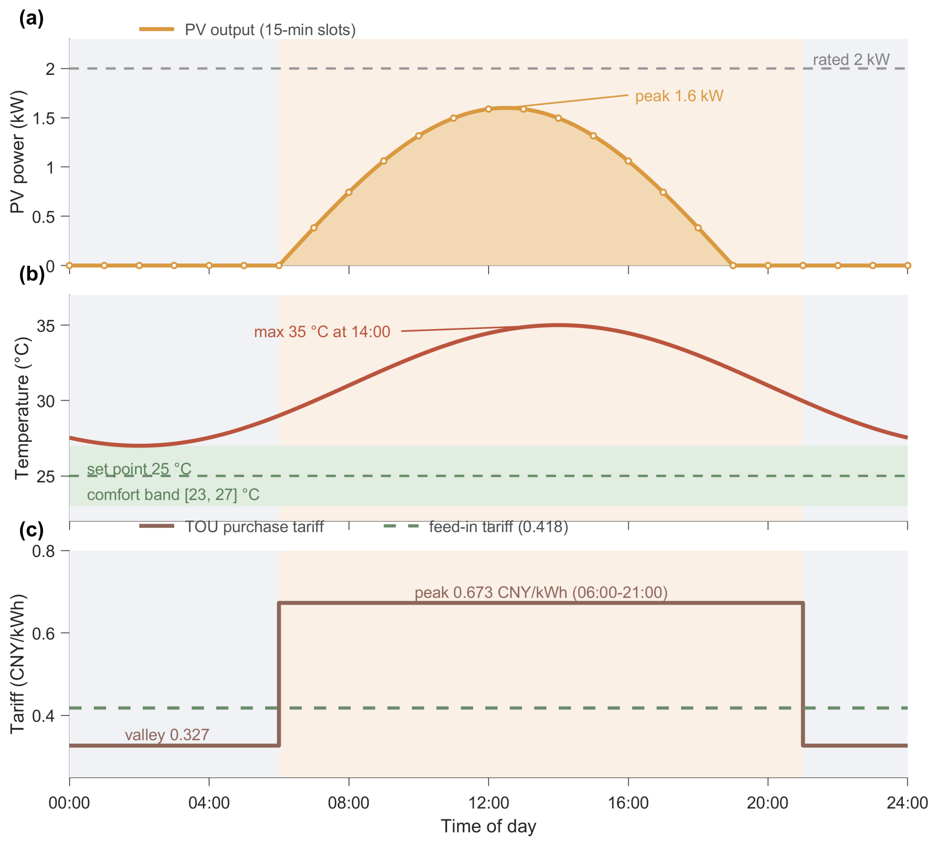
In this case study, a typical household in Southern China during the summer season is considered. The outdoor temperature boundary condition of Equation (10) is taken from typical summer meteorological data for Guangzhou [41], with a daily minimum of about 27 °C in the early morning and a maximum of about 35 °C around 14:00. The PV generation profile shown in Figure 4 corresponds to a clear summer day scaled to the installed capacity. The time-of-use tariff follows the optional residential peak–valley tariff of Guangdong Province [42], and the feed-in remuneration for surplus PV power is set with reference to the provincial benchmark price for surplus electricity from distributed PV. The appliance parameters in

Table 1. Household load parameters.

Load Type	Optimal Start Time	Rated Power (kW)	Operation Duration (h)	Allowable Start-Time Window
Washing machine	17:00	0.8	1	08:00~20:00
Dishwasher	20:00	1	1	18:00~20:00
Air conditioner	─	1.8	16	08:00
Lighting	─	0.1	8	18:00
Rice cooker	─	1.6	0.5	09:00~19:00
Refrigerator	─	0.2	24	00:00
Television	─	0.25	2	19:00

are typical rated values of common household appliances, and the preferred operating windows reflect habitual usage patterns. The parameters are configured as follows:

(1) PV System: A household PV system with an area of 10 m², a photoelectric conversion efficiency of 25%, and a rated power of 2 kW is deployed.

(2) Electricity Tariff: A TOU tariff is applied, where the peak period is 06:00–21:00 with a price of 0.673 CNY/kWh, and the trough period is 21:00–06:00 (the next day) with a price of 0.327 CNY/kWh. The feed-in tariff for surplus PV power is 0.418 CNY/kWh.

(3) Energy Storage System (BESS): The BESS has a capacity of 10 kWh, a maximum charging/discharging power of 1.5 kW, and a round-trip efficiency of 90%, and the operating limits for the SOC are [0.1, 0.9].

(4) EV and HVAC Parameters: The total capacity of the EV battery is 60 kWh; the EV charges and discharges through a home charging pile with a maximum power of 3.3 kW and a charging/discharging efficiency of 0.95; the energy consumption rate is 0.15 kWh/km, the SOC operating range is [0.2, 0.9], the maximum depth of discharge is 0.8, and the next-day departure time is 07:30. For the EV travel model, μ = 3.2 and σ = 0.88 in Equation (4) and μ = 17.6 and σ = 3.4 in Equation (5) are adopted from the statistical modeling of household vehicle travel based on the U.S. National Household Travel Survey [32], which is widely used in residential EV scheduling studies [33]. Although these distributions are fitted to U.S. survey data, the resulting median daily mileage of about 25 km is consistent with reported urban private-car usage intensities in China (typically 20–30 km per day), and the sensitivity analysis in Section 5.4 covers the 12–50 km/day range. Monte Carlo simulation with 1000 samples and a fixed random seed is performed offline; the results reported in Section 5.2 and Section 5.3 correspond to the representative scenario defined by the sample medians (a daily mileage of about 25 km and a return time of 17:36), and the sensitivity of the results to these stochastic parameters is examined in Section 5.4. For the air-conditioning system, the thermal capacity is 0.54 kWh/°C, the thermal resistance is 15 °C/kW, the acceptable temperature band is [23, 27] °C with a preferred set point of 25 °C, and the operating window is 08:00–23:00.

The generation profile of the residential PV system is depicted in Figure 4. The household load parameters are detailed in Table 1, where washing machines and dishwashers are considered as shiftable loads. Temperature-optimized scheduling is shown in Figure 5.

The proposed optimization model involves 0/1 decision variables related to the load start/stop statuses and to the mutually exclusive charging/discharging states of the BESS, the EV, and the grid connection. All constraints are linear except the convex quadratic comfort constraints of Equation (15), so the model constitutes a MIQCP, for which branch-and-bound provides a certified globally optimal solution. The model is implemented in MATLAB (2023b), with YALMIP serving as the modeling interface and GUROBI employed as the solver; the deterministic problem of Equation (26) is solved to a zero optimality gap in less than 10 s per scenario, and the two-stage scenario-based extension of Equations (27) and (28) with K = 10 scenarios is solved in about 40 s on a desktop computer.

5.2. Simulation Results Analysis

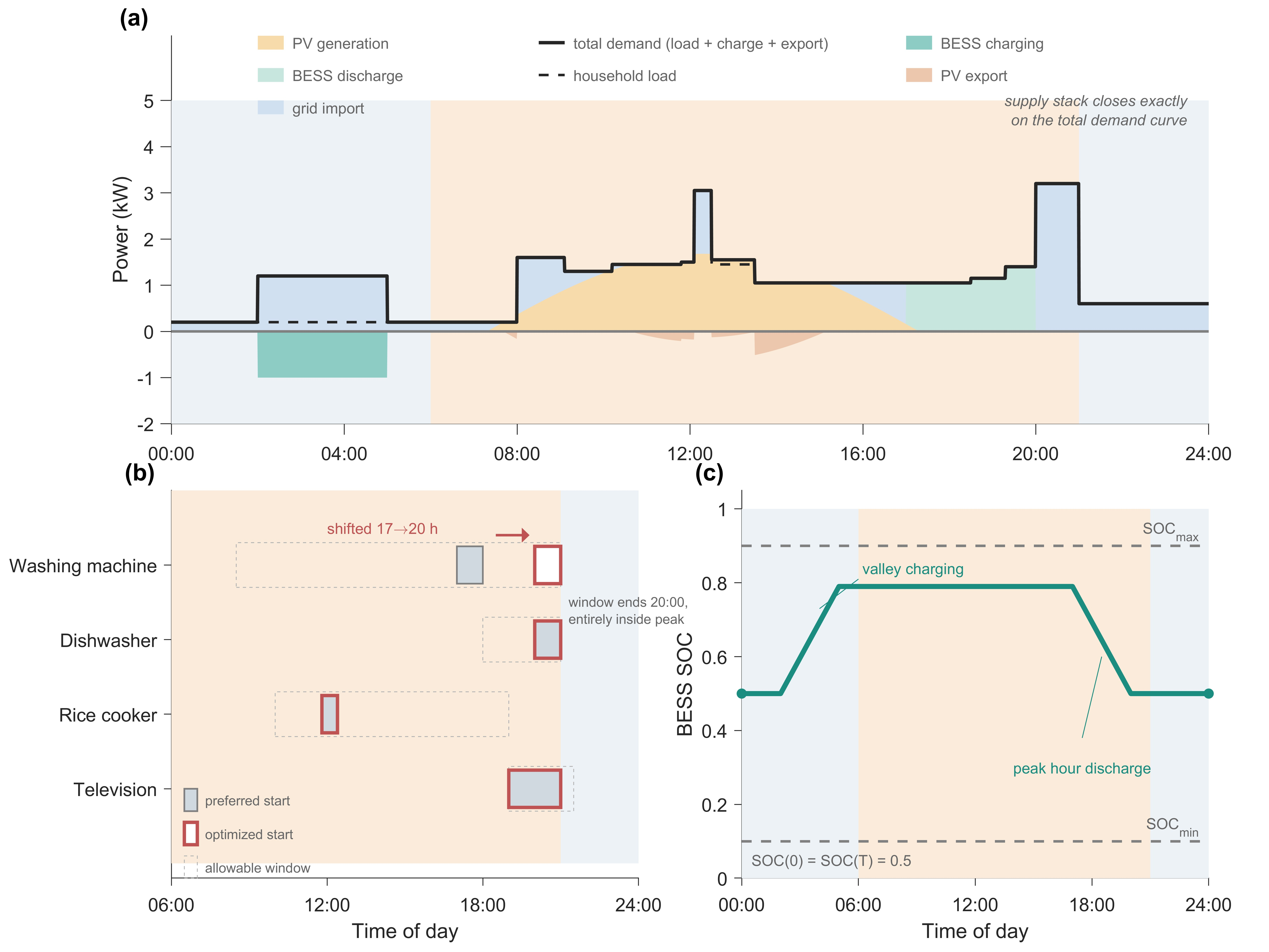
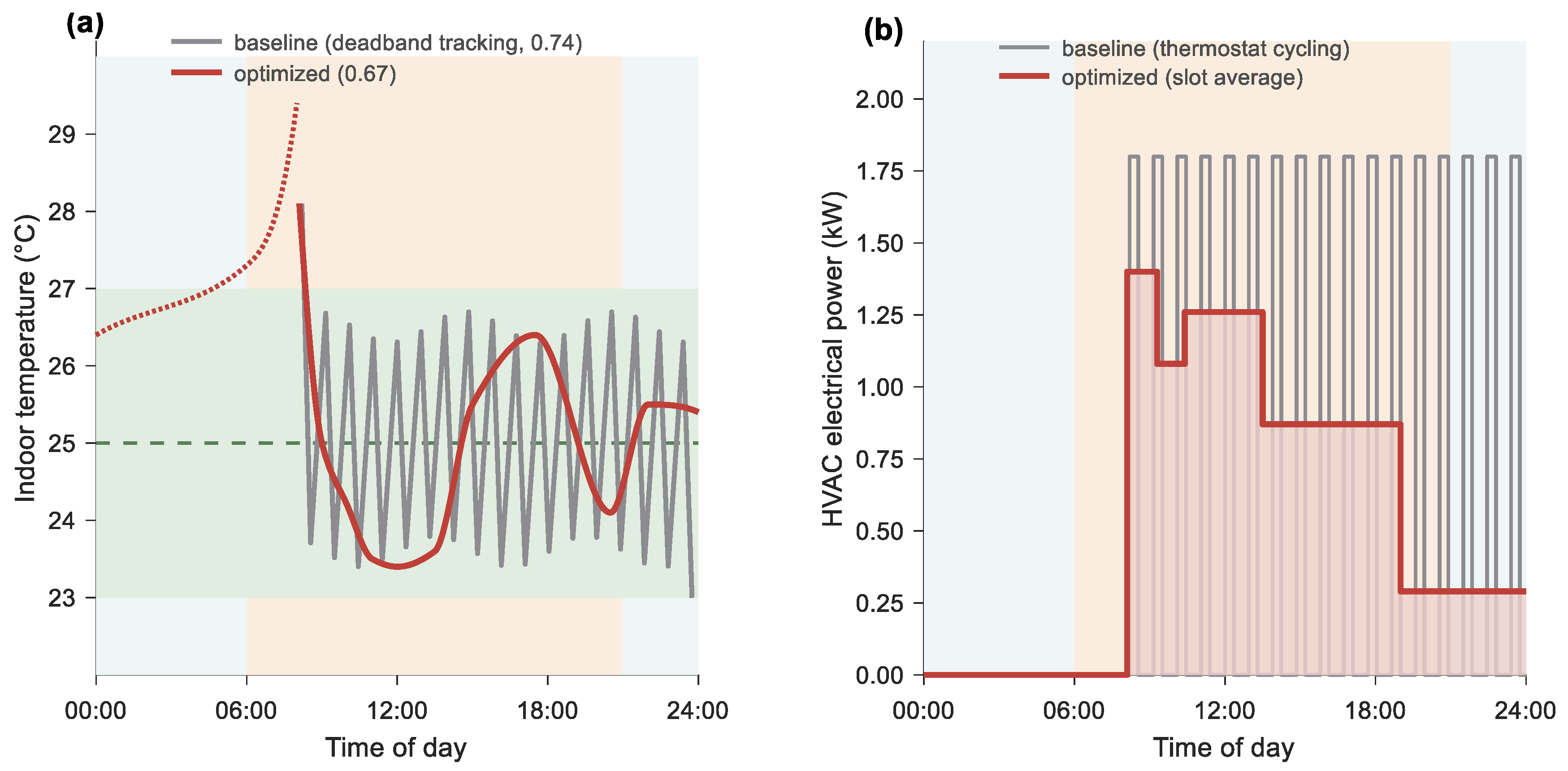
Regarding system energy management, the efficient utilization of PV power is achieved on the load side, where the BESS is charged during periods of PV surplus and discharged during periods of insufficient output at night. Simultaneously, through demand-side management, as illustrated in Figure 6, the operating cycle of the washing machine is shifted from 17:00 to 20:00 to absorb the BESS discharging power, while the dishwasher remains exactly at its preferred start time of 20:00. From an optimization perspective, this demonstrates the algorithm’s capability to intelligently identify the ‘economic–comfort boundary’. Because the dishwasher’s strictly defined admissible window (18:00–20:00) falls entirely within the peak-tariff period, any shifting inside this window would yield exactly zero economic arbitrage. The MIQCP solver correctly determines that sacrificing temporal comfort without corresponding financial compensation is suboptimal, thus perfectly preserving the user’s preference. Furthermore, for the thermostatically controlled load, before optimization the air conditioner cycles within a ±0.85 K deadband around the 25 °C set point, with excursions of up to about 1 °C (thermal comfort 0.74); after optimization, the indoor temperature trajectory is strategically allowed to drift toward the upper boundary of the [23, 27] °C comfort band specifically during the peak-tariff hours. Physically, the scheduling algorithm actively exploits the building’s equivalent thermal inertia (parameterized by R and C in Equation (10)) as a virtual thermal battery. Instead of strictly tracking the 25 °C set point, the HEMS curtails the HVAC’s active compressor power, allowing the room temperature to naturally decay upwards at a rate determined by the outdoor thermal gradient. This thermodynamic relaxation strictly respects the absolute bounds of user tolerance while effectively shifting the electrical cooling demand away from grid stress periods. The cost and comfort index before and after optimization are shown in

Table 2. Costs and comfort indices before and after optimization.

Parameter	Before Optimization	After Optimization
Electricity Cost (CNY)	10.69	9.91
Thermal Comfort	0.74	0.67
Temporal Comfort	1.00	0.91
Electricity Consumption Comfort	0.86	0.77

. Consequently, the thermal comfort indicator structurally drops to 0.67, representing a mathematically optimal compromise. This comprehensive scheme reduces the daily electricity expenditure by approximately 7.3%, from 10.69 CNY to 9.91 CNY. It should be emphasized that this saving is not obtained for free: the electricity-consumption comfort index decreases from 0.86 to 0.77, mainly because the washing machine is displaced by three hours from its preferred start time and the indoor temperature drifts toward the upper comfort limit during peak hours. Whether this degradation is acceptable is ultimately a user-specific judgment; under the adopted weighting (ω₁ = 0.6, ω₂ = 0.4), the comfort index remains above 0.75, and a user who values comfort more highly can increase ω₂, which shrinks both the saving and the comfort loss.

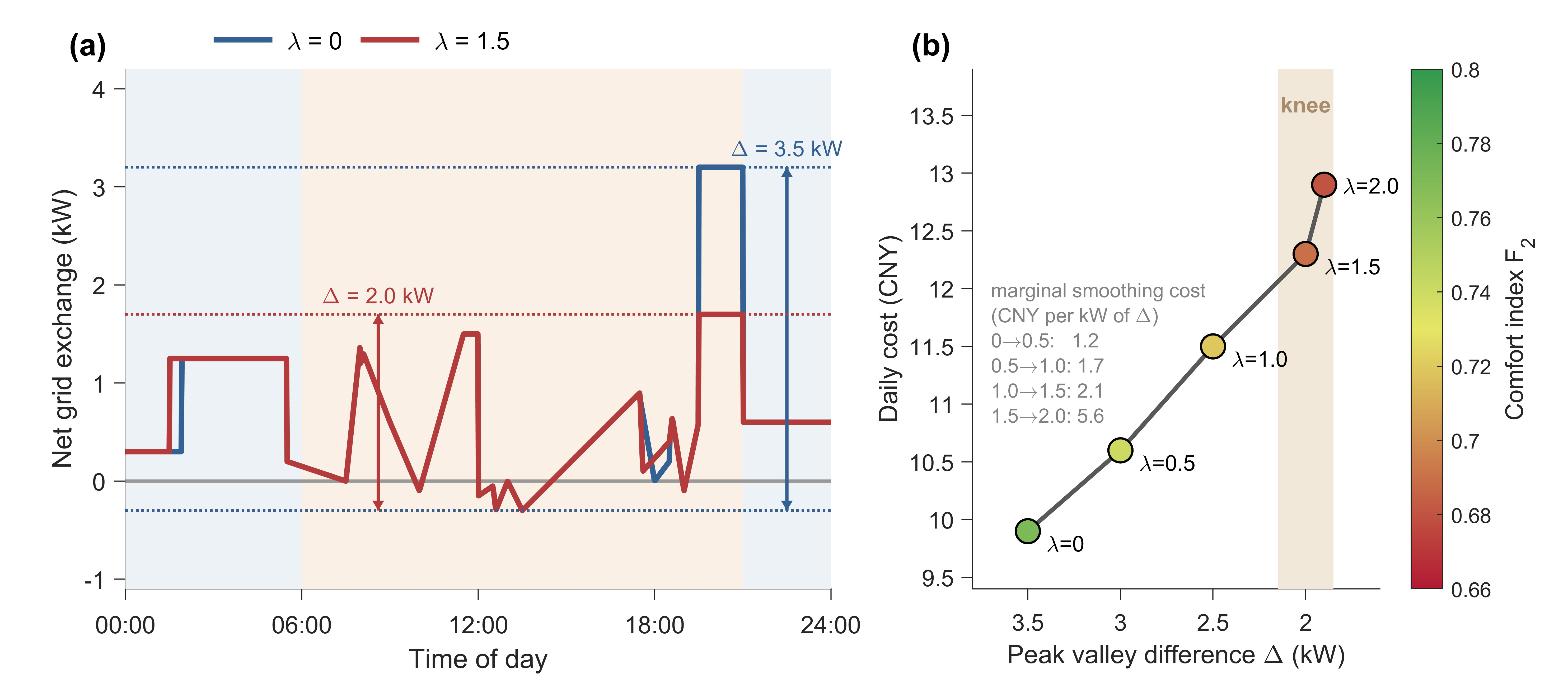
With the introduction of the peak–valley difference penalty coefficient λ, the peak–valley difference of the load curve exhibits a clear convergence trend, as depicted in Figure 7. To characterize the trade-off beyond a single pair of values, the model is solved for λ ∈ {0, 0.5, 1.0, 1.5, 2.0};

Table 3. HEMS optimization results without EV integration.

Parameter	ρ = 0	ρ = 1.5
Peak-to-Valley Difference (kW)	3.5	2
Electricity Cost (CNY)	9.91	12.31
Thermal Comfort	0.67	0.67
Temporal Comfort	0.91	0.74
Electricity Consumption Comfort	0.77	0.70

reports the two boundary cases in detail. The results are summarized in

Table 4. Sensitivity of the scheduling results (without EV) to the peak–valley penalty coefficient λ.

Parameter	λ = 0	λ = 0.5	λ = 1.0	λ = 1.5	λ = 2.0
Peak-to-Valley Difference (kW)	3.5	2.9	2.4	2.0	1.9
Electricity Cost (CNY)	9.91	10.62	11.48	12.31	12.87
Electricity Consumption Comfort	0.77	0.75	0.72	0.70	0.69

. As the λ increases from 0 to 1.5, the peak–valley difference decreases from 3.5 kW to 2.0 kW, while the daily cost rises from 9.91 CNY to 12.31 CNY. The marginal cost of load smoothing grows from about 1.2 CNY/kW at a small λ to about 5.6 CNY/kW beyond λ = 1.5, indicating clearly diminishing returns; λ ≈ 1.0–1.5 constitutes the knee region of the resulting trade-off frontier. It can be inferred that if the power grid aims to guide end users in flattening their load profiles, an economic compensation mechanism must at least offset this cost premium; the marginal-cost values derived from Table 4 provide a direct basis for dimensioning such compensation, and consistent conclusions on aligning household schedules with market-side incentives are reported for prosumer operation planning in retail electricity markets [27].

5.3. Analysis of V2G Strategy

To verify the effectiveness of EVs participating in household energy management, this section presents a comparative analysis between the baseline scenario (Table 3, without EV integration) and the proposed V2G joint optimization scenario (

Table 5. HEMS optimization results considering EV travel and the V2G strategy.

Parameter	ρ = 0	ρ = 1.5
Peak-to-Valley Difference (kW)	4.9	3.5
Electricity Cost (CNY)	5.42	10.67

). It should be noted that Table 3 and Table 4 (household without EV) and Table 5 (household with EV) refer to two different load configurations; the cost premiums of load smoothing reported in Section 5.2 and in this section are therefore defined with respect to different baselines and are not directly comparable.

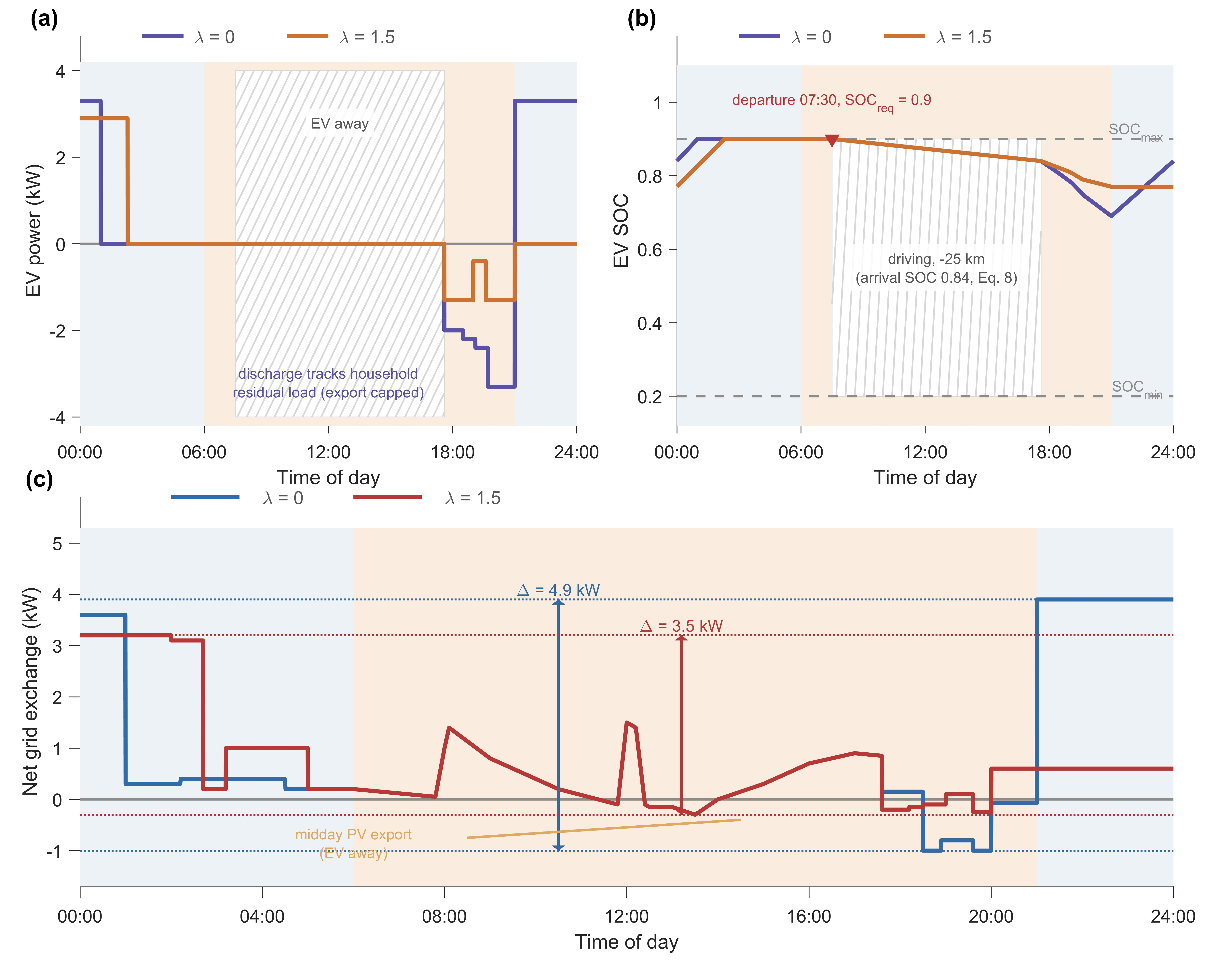
When the system does not incorporate a peak–valley difference penalty mechanism, it exhibits typical purely price-driven behavior. Simulation results demonstrate that in this scenario, the EV fully utilizes its maximum charging and discharging power. During electricity tariff troughs (21:00–06:00), the EV is charged at full power, whereas during peak periods, it discharges power back to the grid (V2G) at the maximum allowable depth of discharge. Although this mode maximizes the user’s arbitrage revenue, it induces significant power fluctuations on the grid side. In particular, the bidirectional power flow enlarges the swing of the net exchange power relative to the no-EV case in Table 3 (from 3.5 kW to 4.9 kW): full-power charging during the night tariff trough raises the maximum import, while peak-hour V2G export drives the net load negative, so the gap between the extremes widens even though the electricity cost falls.

After introducing the peak–valley penalty coefficient λ = 1.5, the objective shifts from purely price-driven arbitrage to a coordinated cost-smoothness optimum. Under this strategy, the high-power charging and discharging behavior of the EV is markedly suppressed. Analytically, the multi-objective formulation dynamically shifts the EV’s role from a ‘grid-scale arbitrage asset’ to a ‘local residual-load tracker’. Since high net grid export now incurs a heavy peak–valley penalty λ, the solver mathematically clips the EV discharge power exactly at the envelope of the household’s residual demand curve. In this mode, the system deliberately foregoes marginal arbitrage revenue; instead, the 60 kWh EV battery is dispatched strictly to self-consume locally, buffering the intermittent spikes of the TCLs. This structural shift effectively mitigates the bidirectional power fluctuations, bounding the grid peak–valley difference at 3.5 kW caused by TCLs such as air conditioning. As shown in Figure 8, the load peak–valley difference is reduced from 4.9 kW to 3.5 kW, i.e., by 1.4 kW, while the daily cost increases from 5.42 CNY to 10.67 CNY. Compared with the no-EV case in Table 3, V2G participation at λ = 0 lowers the daily cost by 4.49 CNY (from 9.91 CNY to 5.42 CNY); it should be noted that this arbitrage benefit would shrink by roughly 20–35% if battery degradation were monetized (Section 4.4), so the reported figures represent an upper bound on the user’s V2G revenue.

To put these figures into perspective at the investment level, the summer-day V2G benefit of 4.49 CNY corresponds, after subtracting the degradation cost of 0.8–1.5 CNY per day estimated in Section 4.4, to a net benefit of roughly 3.0–3.7 CNY per day. Accounting for the seasonal variation examined in Section 5.5 and assuming 330 grid-connected days per year, the annual net benefit amounts to approximately 1000–1200 CNY. Against an incremental hardware cost of 4000–8000 CNY for a bidirectional home charging pile relative to a unidirectional one, the simple payback period is approximately 3.5–7 years, within the typical service life of the equipment, and it shortens further under the wider tariff spreads considered in Section 5.5. The 0.78 CNY/day saving of the no-EV configuration, by contrast, mainly justifies HEMS deployment as an embedded software function of existing smart-home platforms rather than as stand-alone dedicated hardware.

5.4. Value of the Stochastic Extension and Sensitivity to EV Travel Parameters

To ensure a rigorous out-of-sample evaluation, the evaluation in this section utilizes a newly generated, independent set of 1000 Monte Carlo scenarios, distinct from the scenarios used for the K = 10 k-medoids reduction in the optimization stage. A fixed random seed was implemented to guarantee exact reproducibility of both datasets.

Since this work emphasizes EV stochasticity, the dependence of the results on the sampled travel parameters is quantified explicitly. Across the 1000 Monte Carlo scenarios (λ = 0, with V2G), the daily electricity cost has a mean of 7.45 CNY and a standard deviation of 0.62 CNY, and the representative-scenario cost of 7.27 CNY lies close to the distribution median, confirming that the representative scenario is not a favorable outlier.

Table 6. Sensitivity of the daily electricity cost (λ = 0, with V2G) to the EV stochastic travel parameters.

Parameter (Daily Cost in CNY)	Low	Representative	High
EV arrival time	14:12 (6.74)	17:36 (7.27)	21:00 (7.82)
Daily mileage	12 km (6.95)	25 km (7.27)	50 km (7.58)
Arrival SOC	0.70 (7.65)	0.84 (7.27)	0.90 (7.15)

reports one-at-a-time sensitivities in which the EV arrival time, daily mileage, and arrival SOC are varied around their representative values while all other parameters are held fixed. An arrival delayed by one standard deviation (to about 21:00) removes most of the evening-peak discharging window and raises the daily cost by 0.55 CNY; a doubled daily mileage simultaneously reduces the dischargeable energy through Equation (6) and increases the charging demand, raising the cost by 0.31 CNY; and lowering the arrival SOC from its representative value of 0.84, as implied by Equation (8) for the median mileage, to 0.70 raises the cost by 0.38 CNY. In all cases, even with the explicit inclusion of the EV battery degradation penalty, the optimized cost remains well below the no-EV baseline of 9.91 CNY, and the qualitative conclusions regarding the cost–comfort and cost–smoothness trade-offs are unchanged, indicating that the proposed strategy is robust to the EV travel uncertainty. It is worth noting that the above realistic V2G discharging behavior is driven by the incorporation of the degradation costs into the primary objective. Without these penalties, the EV would continuously discharge.

Beyond one-at-a-time sensitivities, the value of explicitly optimizing against travel uncertainty is quantified by comparing the deterministic representative-scenario schedule with the two-stage stochastic schedule of Equations (27) and (28), both evaluated over the same 1000 out-of-sample Monte Carlo scenarios (

Table 7. Out-of-sample comparison of the deterministic and two-stage stochastic schedules.

Metric (1000 Out-of-Sample Scenarios)	Deterministic (Median Scenario)	Stochastic (K = 10, ε = 0.05)
Expected daily cost (CNY)	7.45	7.32
Cost standard deviation (CNY)	0.62	0.48
Mean cost of worst 5% scenarios (CNY)	8.55	7.88
Departure requirement satisfied (%)	91.4	98.3
Solution time (s)	<10	38

). The stochastic schedule lowers the expected daily cost from 7.45 CNY to 7.32 CNY and the cost standard deviation from 0.62 CNY to 0.48 CNY, and it improves the mean cost of the worst 5% of scenarios from 8.55 CNY to 7.88 CNY. Most importantly, the probability of meeting the departure energy requirement rises from 91.4% to 98.3%, at the price of a moderate increase in solution time; the residual violations of the deterministic plan occur almost exclusively in scenarios where the vehicle returns after the scheduled charging window has opened, so that the fixed plan loses part of its charging time. The deterministic schedule therefore remains a reasonable choice when computation is at a premium, whereas the stochastic extension is preferable whenever the punctual availability of the vehicle is critical.

5.5. Generalization Across Seasons and Tariff Structures

To examine whether the conclusions are specific to the summer cooling case, the model is re-solved for two additional configurations: a mild-winter heating day in the same region, in which the HVAC operates in heating mode against an 8–16 °C outdoor temperature profile, and the summer case under a wider residential peak–valley spread of 1.10/0.31 CNY/kWh, representative of provinces with more aggressive time-of-use differentials.

Table 8. Generalization of the main results across seasons and tariff structures (degradation cost included).

Configuration	Cost Saving Without EV (%)	Net V2G Benefit (CNY/day)	Smoothing Premium at λ = 1.5 (CNY)
Summer base case (0.673/0.327 CNY/kWh)	7.3	3.4	5.25
Winter heating case (8–16 °C outdoor)	5.8	2.7	4.10
Widespread tariff (1.10/0.31 CNY/kWh)	10.2	6.0	6.90

summarizes the results with the equivalent degradation cost included at 0.07 CNY/kWh. The qualitative conclusions carry over to both configurations: load shifting yields a 5–10% cost reduction, V2G remains profitable after degradation, and the peak–valley penalty exhibits the same diminishing-returns pattern. Quantitatively, the benefits scale approximately linearly with the tariff spread, indicating that the strategy becomes more attractive precisely in the systems where load smoothing is most valuable; coordinating the household schedule with grid-side energy management, as demonstrated for home–grid coordinated EV charge–discharge management [43], can further increase the utilization of PV energy.

5.6. Comparative Validation of HEMS Strategies

To fully validate the superiority of the proposed framework, a comprehensive comparative analysis is conducted against four baseline strategies commonly discussed in recent literature:

Case 1 (Cost-Minimization Only, CMO): The system purely pursues maximum economic arbitrage without considering the comfort penalty.

Case 2 (Comfort-Maximization Only): Economic costs are entirely deprioritized to maximize the multi-dimensional comfort index.

Case 3 (Deterministic EV Schedule): The stochastic EV travel model is replaced by fixed expected values, as evaluated in Section 5.4.

Case 4 (Conventional 1D Penalty): Represents recent formulations where comfort is modeled simply as a one-dimensional economic penalty (focusing solely on thermal deviation) rather than a normalized multi-dimensional index.

Case 5 (Proposed Strategy): The comprehensive multi-dimensional comfort and EV stochasticity-aware optimization (λ = 0).

As demonstrated in

Table 9. Different scenario comparisons.

Strategy/Case	Daily Cost (CNY)	Thermal Comfort	Temporal Comfort	Comprehensive Comfort	Departure Requirement Satisfied
Case 1: CMO	6.70	0.35	0.45	0.40	98.3%
Case 2: Pure Comfort	12.10	1.00	1.00	1.00	98.3%
Case 3: Deterministic	7.45	0.82	0.72	0.77	91.4%
Case 4: 1D Penalty	6.93	0.89	0.45	N/A (1D penalty)	98.3%
Case 5: Proposed	7.27	0.82	0.72	0.77	98.3%

, the CMO strategy (Case 1) reduces the daily electricity cost to 6.70 CNY. However, this marginal economic gain of 0.57 CNY comes at the cost of severe comfort degradation: schedulable loads are shifted entirely to deep night hours, causing the temporal comfort index to plummet to 0.45, and the comprehensive index drops to an impractical 0.40. Conversely, Case 2 maintains maximum comfort but significantly inflates the operational cost to 12.10 CNY, proving the necessity of a trade-off mechanism.

The necessity of modeling EV stochasticity is explicitly verified by comparing Case 3 and Case 5. The proposed stochastic extension (Case 5) lowers the expected out-of-sample cost compared to the deterministic plan (7.27 CNY vs. 7.45 CNY) while drastically raising the probability of meeting the EV departure requirement from 91.4% to 98.3%. Furthermore, compared to the conventional 1D penalty method (Case 4), which aggressively shifts flexible loads to off-peak hours and neglects temporal user habits, the proposed multi-dimensional index explicitly prevents extreme sacrifice in one domain. The proposed strategy (Case 5) secures a significantly higher temporal comfort index (0.72) and overall comfort index (0.77) while maintaining robust economic savings (7.27 CNY vs. 6.93 CNY of Case 4), thereby preventing the unacceptable user experience inherently caused by simplistic one-dimensional penalties.

Furthermore, a quantitative evaluation of the computational overhead is conducted to ensure the practical feasibility of the proposed framework. As summarized in Table 9, although the proposed multi-dimensional comfort index (Case 5) introduces additional variables and constraints compared to the conventional 1D penalty method (Case 4), it is meticulously formulated to preserve the Mixed-Integer Quadratically Constrained Programming (MIQCP) structure. Using the GUROBI solver, the average simulation time for the conventional 1D penalty scheduling (Case 4) is approximately 1.25 s. In comparison, the proposed multi-dimensional strategy (Case 5) requires an average simulation time of 1.58 s. This indicates that while the multi-dimensional comfort constraints incrementally increase the computational burden, the absolute simulation time remains strictly within a couple of seconds. Such a marginal overhead (an increase of approximately 0.33 s) is entirely negligible for a day-ahead (and even intra-day) scheduling framework, proving that the proposed strategy successfully achieves significant improvements in multi-dimensional user comfort without compromising computational tractability.

6. Conclusions

In this paper, a home energy management strategy considering EV travel randomness is proposed to address the coordinated optimization between economic efficiency and multi-dimensional comfort in a residential PV-BESS. By establishing a bounded comfort aggregation model and an offline-decoupled EV sequential control logic, a mixed-integer convex optimization model is constructed and solved to proven global optimality. Based on the simulation analysis, the main conclusions are drawn as follows:

Quantification of the economic–comfort trade-off: The proposed strategy effectively time-shifts flexible loads, reducing the daily residential electricity expenditure by approximately 7.3%. Meanwhile, the electricity-consumption comfort index remains within an acceptable range (decreasing moderately from 0.86 to 0.77), explicitly validating the cost of comfort preservation.

Mitigation of grid-side power fluctuations: The peak–valley difference penalty mechanism successfully prevents severe power fluctuations induced by purely price-driven EV arbitrage. Achieving a cost–smoothness optimum reduces the household load peak–valley difference by 1.4 kW for a marginal cost premium of 5.25 CNY, indicating the necessity of designing economic compensation mechanisms on the distribution network side.

Robustness against EV travel uncertainty: Internalizing EV travel uncertainty via the two-stage scenario-based framework significantly secures the scheduling. Compared to deterministic approaches, the expected out-of-sample daily cost drops to 7.32 CNY, and the probability of satisfying EV departure energy requirements increases from 91.4% to 98.3% under a 5% risk budget, offering practical investment viability with a payback period of 3.5–7 years.

It is important to acknowledge the limitations of the current study. The proposed framework assumes perfect day-ahead forecasts for PV generation and outdoor temperature to maintain computational tractability while strictly addressing the spatial–temporal uncertainties of EVs and the nonlinear multi-dimensional comfort index. In real-world applications, meteorological conditions are highly stochastic. Introducing full scenario-based stochastic programming for continuous PV and temperature variables into the current two-stage MIQCP model would lead to the curse of dimensionality, exponentially increasing the computational burden. Therefore, our future work will focus on developing a multi-timescale scheduling framework. By integrating Model Predictive Control (MPC) or robust optimization at the intra-day operational stage, we aim to dynamically compensate for real-time PV and temperature forecast errors without compromising the global optimality of the day-ahead scheduling.

Furthermore, regarding the practical implementation of the HEMS, while the proposed two-stage MIQCP framework effectively handles EV stochasticity in the day-ahead phase via offline Monte Carlo sampling, real-time EV availability may occasionally experience extreme deviations from the predetermined representative scenarios (e.g., unexpected late arrivals or severe energy deficits). As a crucial future extension, a real-time dynamic adjustment mechanism will be integrated. This multi-timescale mechanism will employ rule-based sequential logic to adjust dispatch dynamically: in scenarios of severe EV energy deficits, the HEMS will instantly suspend V2G arbitrage and prioritize forced grid-charging to secure departure requirements; conversely, during unexpected energy surpluses, opportunistic V2H discharging will be dynamically unlocked to support flexible loads. While the current study establishes a robust, bottom-up operational framework for a single residential prosumer, realizing comprehensive market-based compensation requires scaling this model to a macroscopic level. Therefore, our future research will extend this framework to a multi-node distribution network level to evaluate grid-side impacts within an aggregator-based transactive energy market.

Finally, the accuracy and precision of the proposed day-ahead strategy are inherently bounded by the static nature of the forecasted household load profiles. Under a highly dynamic and variable load model, high-frequency fluctuations—such as the sudden, stochastic activation of uncoordinated high-power appliances—would introduce real-time deviations from the predetermined 15 min dispatch set points. While these dynamic perturbations marginally reduce the precision of thermal comfort tracking and expected economic arbitrage, the integrated PV-BESS physically functions as an energy buffer, absorbing instantaneous intra-slot power mismatches to mitigate severe operational impacts. To fundamentally enhance the scheduling accuracy and precision against highly variable load profiles, coupling the proposed day-ahead MIQCP framework with an intra-day, rolling-horizon MPC layer will be a crucial direction for our future research.

7. Materials and Methods

While writing this article, the authors used Gemini (3.1Pro) to help with language polishing and flowchart code generation, as well as the syntax for MATLAB/YALMIP (2023b) scheduling code. All code logic, mathematical formulas, and results were independently verified, implemented, and interpreted by the authors, who take full responsibility for this work.