Nonlinear Wave Modeling of Internally Heat-Integrated Air Separation Columns via Local Mechanism-Based Optimization

Abstract

Compared with conventional air separation columns, the internally heat-integrated air separation column (HIASC) offers superior energy efficiency. However, its structural complexity poses significant challenges for model-based online optimization and control. This study proposes a nonlinear wave model based on a model updating strategy, which substantially reduces modeling complexity. First, wave propagation theory is employed to characterize the concentration distribution profiles and their propagation velocities within the HIASC. Subsequently, a localized analytical method based on the distributed wave velocity is developed from local mechanistic insights to evaluate waveform distortion. Furthermore, a model updating strategy is introduced, which determines the optimal updating frequency according to the degree of waveform deformation, thereby mitigating computational redundancy caused by excessive updates. Finally, the proposed strategy is integrated into the nonlinear wave model to achieve an optimal balance between accuracy and computational efficiency. Simulation results validate the effectiveness and robustness of the proposed modeling approach.

1. Introduction

Air separation technology plays a pivotal role across a diverse range of industries, encompassing traditional sectors such as petrochemicals [1,2] and metallurgy [3], as well as healthcare [4], and extending to various modern energy industries [5,6,7]. Entering the 21st century, humanity is confronted with unprecedented challenges and opportunities. Against the global imperative to mitigate climate change and pursue carbon neutrality, air separation technology has assumed a new mission, emerging as a critical enabler within the clean energy and carbon neutrality framework [8,9]. Concurrently, the rapid advancement of high-tech industries, including semiconductors and new energy, has imposed increasingly stringent requirements on both the production capacity and purity of industrial gases [10].

The internally heat-integrated air separation column (HIASC) investigated in this study employs cryogenic distillation. Currently, cryogenic distillation remains the preferred technology for large-scale production of high-purity nitrogen and oxygen. The co-production of these gases significantly enhances energy efficiency while reducing operational costs [11]. However, conventional air separation columns incur substantial energy consumption during the distillation process [12,13]. To mitigate this drawback, several researchers have introduced internally heat-integrated technology into conventional columns [14,15,16,17], which constitutes the primary focus of this work. This technology offers distinct advantages in terms of energy reduction and efficiency improvement [16,18,19]. Specifically, during the heat exchange process, the ascending vapor in the rectifying section is utilized to heat the descending liquid in the stripping section. This integration generates internal reflux in the rectifying column and internal vapor flow in the stripping column, thereby alleviating the thermal load on the condenser and improving overall energy efficiency by over 30% [17,20]. Yan et al. developed a first-principles model of the HIASC based on mass and energy conservation laws and thermally coupled principles. Their study demonstrated that, compared with conventional columns, this model achieves an energy saving of approximately 47% [17]. Similarly, Chang established a rigorous mathematical model for the HIASC and proposed a novel structural configuration capable of simultaneously producing high-purity oxygen and nitrogen. Research indicates that this optimized HIASC structure facilitates more efficient energy utilization compared to conventional cryogenic air separation columns [21,22].

Mechanism-based modeling approaches can effectively construct accurate representations of HIASC systems, thereby providing valuable theoretical guidance for research. However, these first-principles models entail extensive material balance calculations and differential operations, characterized by a large number of differential variables and equations. This complexity poses significant challenges for application scenarios requiring real-time computation, such as online monitoring and control system design, where low-latency feedback is imperative. The computational burden associated with complex models hinders the efficiency of real-time operational strategies. Consequently, real-time model deployment necessitates an optimal trade-off between model accuracy and computational efficiency [23,24,25].

The nonlinear wave theory in separation processes offers a viable paradigm for developing models that reconcile high accuracy with computational efficiency [25,26]. Wave phenomena are ubiquitous in separation processes, meaning that during mass and heat transfer, the profiles of specific parameters, such as component concentration and temperature, maintain a fixed shape and propagate during dynamic processes [27,28]. Wave phenomena also exist in distillation and air separation processes. Extensive studies by Hwang [26], Marquardt [29], Kienle [30], and Zhu [31] et al. have demonstrated that the different steady states of a distillation column can be characterized by the positions of distinct constant waves. Kienle developed a low-order wave model and benchmarked its predictive performance against conventional models for ternary and quinary mixtures. The results indicated that the low-order wave model yielded high accuracy in capturing dynamic characteristics under most operating conditions [30].

Hankins extended the research on nonlinear wave models for distillation columns by incorporating the effects of enthalpy, liquid holdup, and reflux into both theoretical derivations and experimental validations [27]. They concluded that for systems involving mixtures of arbitrary components, all potential transient waves or steady states can be resolved into n−1 correlated waveforms. Bian proposed a novel methodology for the online estimation of wave model parameters and analyzed the interrelationships between tray concentration predictions, parametric sensitivity, and system stability [32,33].

Heat-integrated distillation columns exhibit strong nonlinearity and complex dynamic coupling due to heat exchange between the rectifying and stripping sections. This configuration is significantly more complex than that of conventional distillation columns. Consequently, many foundational assumptions of classical wave theory no longer hold for heat-integrated distillation columns. For instance, the constant molar overflow assumption (i.e., constant molar vapor and liquid flows on each tray) and the assumption of an invariant wave shape are invalid. This invalidates the waveform velocity equations derived from conventional wave theory. In the context of internally heat-integrated distillation, Liu observed that applying wave theory requires accounting for the impact of waveform transformation on propagation velocity. Based on this insight, a comprehensive nonlinear wave model was established and applied to an ideal benzene-toluene mixture to elucidate component prediction and dynamic behavior [34]. Schulze employed wave theory to construct a reduced-order model, which significantly simplifies the model structure and facilitates its implementation in Model Predictive Control (MPC) architectures [35]. The approach demonstrates considerable performance improvements in air separation units, fully substantiating the effectiveness of wave theory.

The separation of ideal systems involves relatively straightforward vapor–liquid equilibrium relationships. In contrast, air separation constitutes a non-ideal separation process characterized by more complex physicochemical properties, necessitating a re-examination of these relationships. In our previous work, we proposed a modeling method for HIASC based on nonlinear wave theory. This approach can effectively reduce the complexity of first-principles models while maintaining high model accuracy, thereby meeting the requirements for subsequent real-time monitoring or control [36].

While the nonlinear wave model-based strategy for HIASC significantly reduces modeling complexity, it also introduces new challenges. Although our 2023 study [13] successfully applied wave theory to HIASC, it relied on the conventional distillation assumption of wave profile invariance (notably in the wave velocity equation), potentially causing model deviations. The assumption of wave profile invariance is similarly adopted in an earlier study [23], potentially leading to comparable model deviations. Furthermore, numerous waveform parameters within the model must be determined via online optimization. Updating these parameters at every sampling interval imposes a substantial computational burden, whereas infrequent updates risk model mismatch and a subsequent degradation in accuracy. To address this dilemma, this study proposes a novel modeling framework designed to achieve an optimal trade-off between accuracy and computational efficiency. We first adopt the global nonlinear wave model of the HIASC grounded in wave propagation theory. Building upon this foundation, a local mechanism-based analytical method is proposed to quantitatively characterize the distinct propagation velocities of concentration waves across individual trays. This method evaluates the degree of waveform distortion to determine the necessity of parameter updates, thereby circumventing the computational redundancy associated with frequent adjustments. Subsequently, a nonlinear optimization model incorporating a parameter updating mechanism is established. By strategically tolerating a marginal sacrifice in accuracy, the model effectively reduces computational costs while significantly enhancing operational speed. Simulation results demonstrate that the proposed model achieves a substantial improvement in computational efficiency without compromising accuracy to any significant extent.

2. Modeling of HIASC Based on Wave Theory

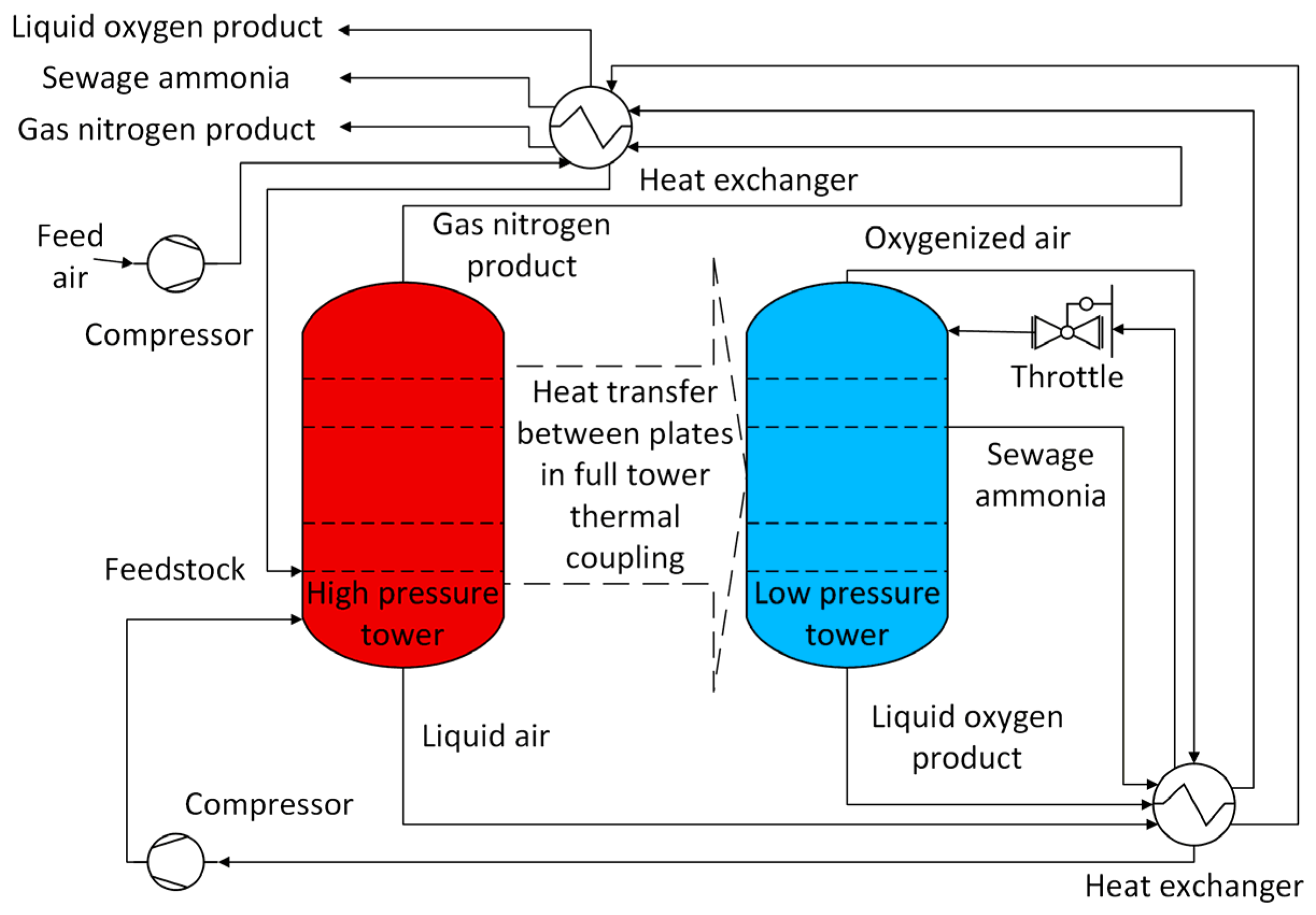
Wave theory has been successfully applied to model conventional air separation columns, demonstrating high accuracy. However, the structural configuration of the HIASC is significantly more complex than that of its conventional counterpart. Consequently, applying wave theory to the HIASC requires a re-evaluation of its internal mass transfer mechanisms, based on which a tailored wave model can be established. The structural schematic of the HIASC is shown in Figure 1.

The HIASC has a relatively large number of trays, and its local mass transfer characteristics are similar to the continuous mass transfer characteristics of a packed column. Its mass transfer process can be described by the following differential equations [13,36]:

$${\displaystyle \frac{\partial x_i}{\partial t}}-{\displaystyle \frac{\partial x_i}{\partial s}}=-MT({y_i}^{*}\left(x_i\right)-y_i)$$

(1)

$${\displaystyle \frac{V}{L}}{\displaystyle \frac{\partial y_i}{\partial s}}=MT({y_i}^{*}\left(x_i\right)-y_i)$$

(2)

Here, $x_i$ and $y_i$ denote the concentrations in the liquid and gas phases, respectively. The parameter $MT$ represents the dimensionless mass transfer coefficient, while $V$ and $L$ correspond to the molar flow rates of the gas and liquid phases. The term $y_i^{*}\left(x_i\right)$ defines the vapor–liquid equilibrium relationship, and $s$ stands for the dimensionless spatial coordinate. The subscript $i$ indicates the specific components involved: oxygen, nitrogen, and argon.

Under the assumption of steady-state conditions (i.e., $\partial x/\partial t=0$), an integral transformation is applied to Equation (1). This transforms the original coordinate system into a moving $\epsilon -t$ sub-coordinate system traveling at velocity $v$, defined as follows:

$$\epsilon =s-s^{\prime }$$

(3)

$$s^{\prime }=\int vdt$$

(4)

By substituting Equations (3) and (4) into Equations (1) and (2), the following equations can be obtained:

$$(1+v){\displaystyle \frac{\partial x_i}{\partial \epsilon }}=MT({y_i}^{*}\left(x_i\right)-y_i)$$

(5)

$${\displaystyle \frac{V}{L}}(1+v){\displaystyle \frac{\partial y_i}{\partial \epsilon }}=MT({y_i}^{*}\left(x_i\right)-y_i)$$

(6)

Equation (7) is derived from Equations (5) and (6), which is expressed as:

$$\epsilon -\int {\displaystyle \frac{(1+v)dx}{MT(C_1+{y_i}^{*}\left(x_i\right)-L{x}_i/v)}}+C_2=0$$

(7)

Here, $C_1$ and $C_2$ denote the integration constants arising from the indefinite integration of Equations (5) and (6). Directly solving for $x_i$ from Equation (7) presents significant challenges. In our previous work [36], a fractional description approximation was used for the vapor–liquid equilibrium relationship. However, such a description is more consistent with the vapor–liquid equilibrium relationship of ideal systems. Since air separation belongs to non-ideal systems, a more general quadratic polynomial is adopted here to describe the equilibrium relationship: $y_i^{*}\left({\widehat{x}}_i\right)=A{{\widehat{x}}_i}^2+B{\widehat{x}}_i+C.$ Subsequently, the integrand in Equation (7) is manipulated via the method of completing the square, resulting in the following expression:

$${\displaystyle \frac{1+v}{B\left(C_1+y_i^{*}\left({\widehat{x}}_i\right)-\frac{L{x}_i}{V}\right)}}={\displaystyle \frac{1}{p\left({\widehat{x}}_i-p_1\right)\left({\widehat{x}}_i-p_2\right)}}$$

(8)

where $p$, $p_1$, and $p_2$ represent the factorization parameters.

Substituting Equation (8) into Equation (7) and performing the integration yields the expression for $x_i$, which is the description function of the component concentration waveform:

$${\widehat{x}}_i=p_2+{\displaystyle \frac{p_1-p_2}{1+e^{p_3\left(\epsilon +p_4\right)}}}$$

(9)

where $p_1$, $p_2$, $p_3$, and $p_4$ represent the structural parameters of the concentration curve. Transforming the above equation back to the original coordinate system, we obtain:

$${\widehat{x}}_i=p_2+{\displaystyle \frac{p_1-p_2}{1+e^{p_3\left(s-S\right)}}}$$

(10)

where $S$ denotes the point of most drastic change in the concentration curve, i.e., the inflection point. The parameters $p_1$, $p_2$, and $p_3$ possess actual physical meanings: $p_1$ and $p_2$ represent the maximum and minimum asymptotic concentrations in the component concentration waveform description function, respectively, while $p_3$ represents the slope characteristic quantity at the inflection point position. Therefore, the description function for the component concentration waveform of the rectifying and stripping sections of the HIASC can be obtained:

$${\widehat{X}}_{i,j}=X_{i,r\_min}+{\displaystyle \frac{X_{i,r\_max}-X_{i,r\_min}}{1+e^{-k_r\left(j-S_r\right)}}} j=\mathrm{1,2},\dots ,{\displaystyle \frac{n}{2}}$$

(11)

$${\widehat{X}}_{i,j}=X_{i,s\_min}+{\displaystyle \frac{X_{i,s\_max}-X_{i,s\_min}}{1+e^{-k_s\left(j-S_s\right)}}} j=f,f+1,\dots ,n$$

(12)

Here, ${\widehat{X}}_{i,j}$ denotes the concentration measurement at the $j$-th tray. The terms $X_{i,r\_max}$, $X_{i,r\_min}$, $k_r$, $X_{i,s\_max}$, $X_{i,s\_min}$, and $k_s$ serve as waveform parameters, while $S_r$ and $S_s$ identify the inflection point locations within the concentration profiles of the rectifying and stripping sections, respectively. These distribution parameters carry specific physical significance: $X_{i,r\_min}$ and $X_{i,s\_min}$ correspond to the minimum asymptotic concentrations for the rectifying and stripping sections. Similarly, $X_{i,r\_max}$ and $X_{i,s\_max}$ represent their respective maximum asymptotic concentrations. The coefficients $k_r$ and $k_s$ act as characteristic slope indicators at the inflection points, reflecting the steepness of the curve without being identical to the geometric slope.

Throughout the dynamic variation process, parameters such as $X_{i,r\_max}$, $X_{i,r\_min}$, $k_r$, $X_{i,s\_max}$, $X_{i,s\_min}$, and $k_s$ remain relatively stable and do not exhibit significant fluctuations. Consequently, it is reasonable to assume that the time derivatives of these variables are zero. This assumption streamlines the derivation without compromising result accuracy. By differentiating both sides of Equations (11) and (12) with respect to time, we obtain the relationship linking the component concentration change on each tray to the velocity of the inflection point:

$${\displaystyle \frac{d{\widehat{X}}_{i,j}}{dt}}={\displaystyle \frac{-k_r(X_{i,r\_max}-X_{i,j})(X_{i,j}-X_{i,r\_\mathrm{m}\mathrm{i}\mathrm{n})}}{X_{i,r\_max}-X_{i,r\_min}}}{\displaystyle \frac{d{S}_r}{dt}}$$

(13)

$${\displaystyle \frac{d{\widehat{X}}_{i,j}}{dt}}={\displaystyle \frac{-k_s(X_{i,s\_max}-X_{i,j})(X_{i,j}-X_{i,s\_\mathrm{m}\mathrm{i}\mathrm{n})}}{X_{i,s\_max}-X_{i,s\_min}}}{\displaystyle \frac{d{S}_s}{dt}}$$

(14)

The material balance equations for each tray of the HIASC are as follows:

$$H{\displaystyle \frac{d{X}_{i,1}}{dt}}=-(V_1+G_1)y_{i,1}-{(L}_1+U_1)x_{i,1}+V_2{y}_{i,2}+F_1{z}_{i,1}$$

(15)

$$H{\displaystyle \frac{d{X}_{i,j}}{dt}}=L_{j-1}{x}_{i,j-1}-(V_j+G_j)y_{i,j}-{(L}_j+U_j)x_{i,j}+V_{j+1}{y}_{i,j+1}+F_j{z}_{i,j}$$

(16)

$$H{\displaystyle \frac{d{X}_{i,n}}{dt}}=L_{j-1}{x}_{i,j-1}-(V_j+G_j)y_{i,j}-{(L}_j+U_j)x_{i,j}+F_j{z}_{i,j}$$

(17)

Here, the index $i$ refers to specific gas components (nitrogen, oxygen, and argon), while $j$ indicates the tray number and $n$ stands for the total number of trays. The variable $H$ denotes the liquid holdup on a tray. Concentrations in the liquid and vapor phases are represented by $x$ and $y$, respectively. Furthermore, $L$ and $V$ correspond to the molar flow rates of the liquid and vapor streams. The terms $G$ and $U$ signify the side-stream withdrawal rates for the vapor and liquid phases, respectively. Finally, $F$ represents the total feed flow rate entering the system, and $z$ indicates the component concentration of the feed.

${\widehat{X}}_j$ is the observed value of $X_j$, and ${\displaystyle \frac{d{\widehat{X}}_{i,j}}{dt}}\approx {\displaystyle \frac{d{X}_{i,j}}{dt}}$. Substituting Equations (13) and (14) into the HIASC material balance Equations (15)–(17), performing addition operations on the trays of the rectifying section and the stripping section, and through mathematical transformation, the movement velocity formulas for the component concentrations of the HIASC are obtained as follows:

$${\displaystyle \frac{d{S}_{i,r}}{dt}}={\displaystyle \frac{V_{\frac{n}{2}+1}{y}_{\frac{n}{2}+1}-V_1{y}_{i,1}-L_{\frac{n}{2}}{x}_{i,\frac{n}{2}}+{\sum }_{j=1}^{\frac{n}{2}}{(F}_j{z}_{i,j}-G_j{y}_{i,j}-U_j{x}_{i,j})}{-H{\sum }_{j=1}^{\frac{n}{2}}\frac{k_r\left(X_{i,r\_\mathit{max}}-X_{i,j}\right)\left(X_{i,j}-X_{i,r\_min}\right)}{X_{i,r\_max}-X_{i,r\_min}}}}$$

(18)

$${\displaystyle \frac{d{S}_{i,s}}{dt}}={\displaystyle \frac{L_{\frac{n}{2}}{x}_{\frac{n}{2}}-V_{\frac{n}{2}+1}{y}_{i,\frac{n}{2}+1}-L_n{x}_{i,n}+{\sum }_{j=\frac{n}{2}+1}^n{(F}_j{z}_{i,j}-G_j{y}_{i,j}-U_j{x}_{i,j})}{-H{\sum }_{j=\frac{n}{2}+1}^n\frac{k_s\left(X_{i,s\_\mathit{max}}-X_{i,j}\right)\left(X_{i,j}-X_{i,s\_min}\right)}{X_{i,s\_max}-X_{i,s\_min}}}}$$

(19)

$y_{i,j}$ represents the concentration of the gaseous light component, which is calculated based on the vapor–liquid equilibrium relationship:

$$y_{i,j}=k_{i,j}{x}_{i,j}$$

(20)

where $k$ is the vapor–liquid equilibrium coefficient.

Heat coupling equation:

$$Q_j=U_{ov}A\Delta T_j$$

(21)

$U_{ov}$ denotes the heat transfer coefficient of the tray, $A$ represents the heat transfer area, and $\Delta T_j$ indicates the temperature difference between two thermally coupled trays.

To improve the accuracy of the model, we no longer use the constant molar overflow assumption to calculate vapor and liquid molar flow rates. Instead, the variation in the molar flow on each tray is fully taken into account during the modeling process. The specific flow relationships are as follows:

$$L_j={\displaystyle \frac{Q_j}{\lambda }}+L_{j-1}+F_j{q}_j-U_j$$

(22)

$$V_j={\displaystyle \frac{Q_j}{\lambda }}+V_{j+1}+F_j{(1-q}_j)-G_j$$

(23)

where $\lambda$ is the latent heat of vaporization, and $q$ is the feed thermal condition.

The concentration profile movement velocity Equations (18) and (19), the concentration profile description Functions (11) and (12), the vapor–liquid equilibrium Equation (20), the heat coupling Equation (21), and the vapor–liquid molar flow rate calculation Equations (22) and (23) collectively constitute the nonlinear dynamic model of the HIASC based on the wave theory. For the convenience of subsequent descriptions, we will refer to this model simply as the wave model.

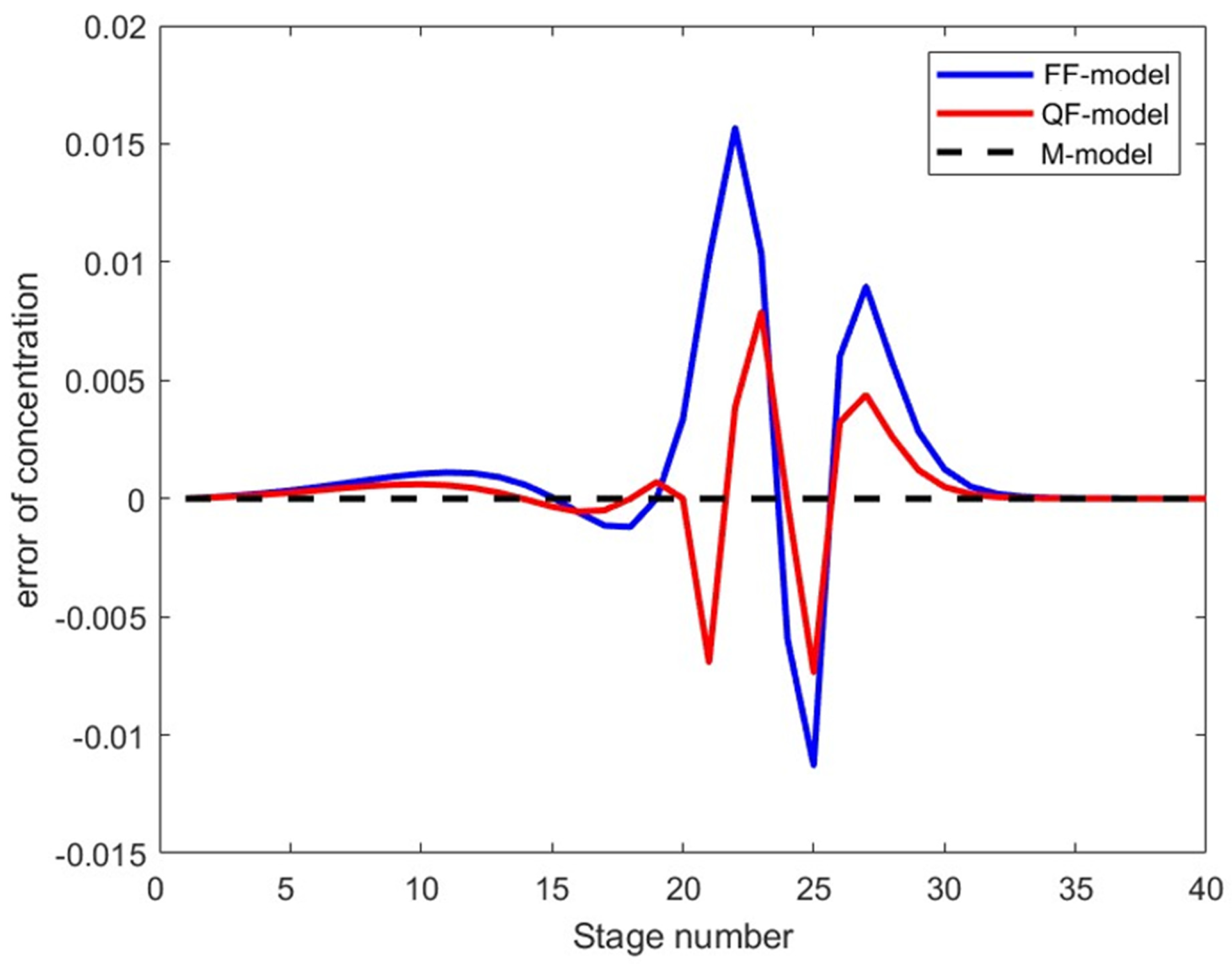
A brief comparison of the steady-state and dynamic performance between the proposed model and our previous model [36] is presented. The steady-state comparison of tray compositions under initial conditions is shown in Figure 2, which was created using Matlab software (Matlab 2024a).

The M-model serves as the mechanism-based benchmark model [16,17]. The FF-model represents the model error associated with the fractional vapor–liquid equilibrium (VLE) relationship, while the QF-model corresponds to the error based on the quadratic VLE relationship. As shown in Figure 2, the proposed model exhibits smaller errors in concentration observations across various trays compared to the previous model, indicating improved accuracy. This demonstrates that the proposed model outperforms the previous model in describing the steady-state concentration distribution profiles.

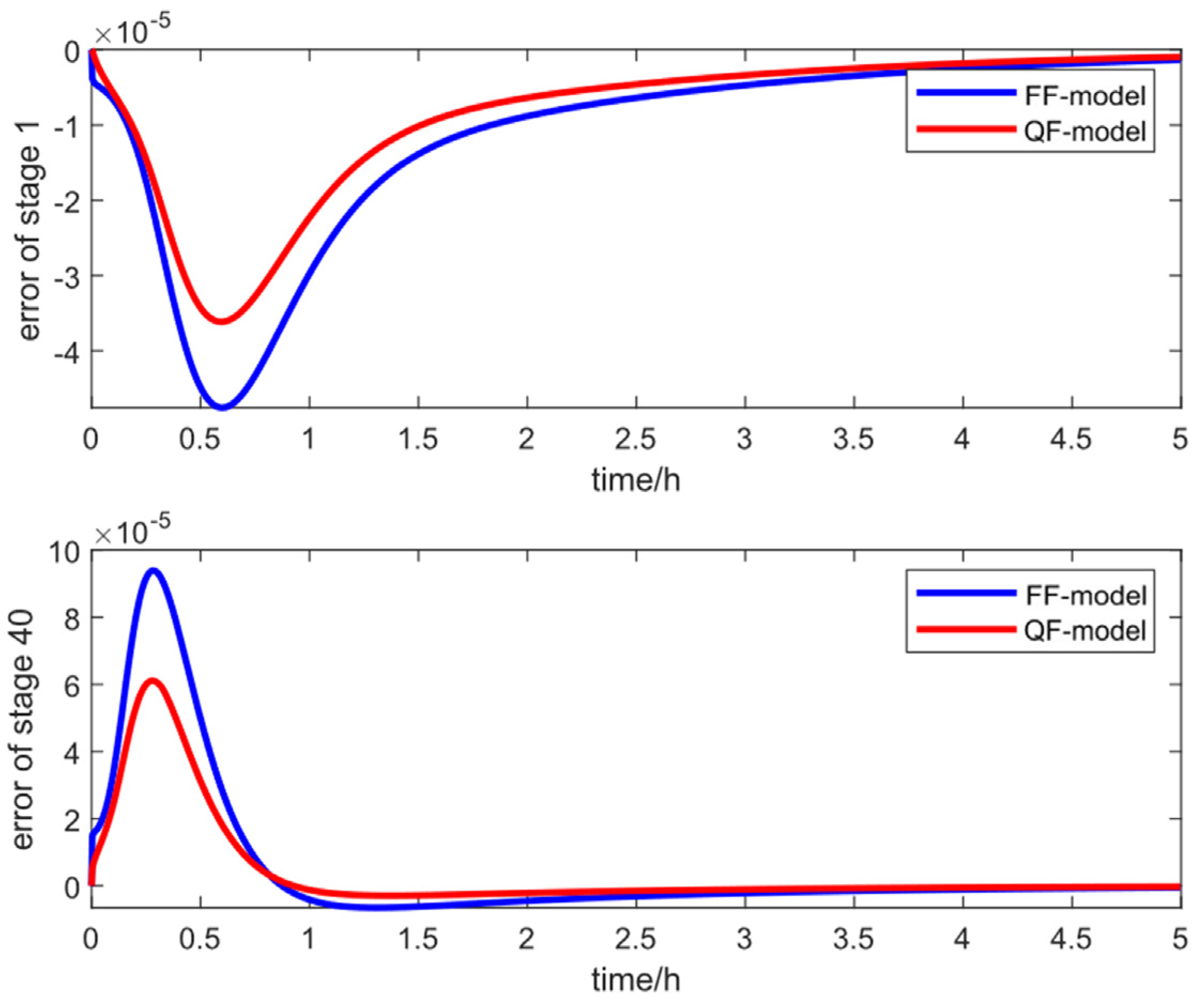
Figure 3 shows the dynamic concentration tracking errors of the two models under a 10% flow increase. It can be observed that the QF-model exhibits a smaller maximum error during the transient process, indicating that the dynamic performance is also improved compared to the previous model.

3. Study on the Movement Law of Concentration Distribution Curves Based on Local Mechanism Analysis

3.1. Local Qualitative Analysis of Component Concentration Profiles

As illustrated in Figure 4, when the feed thermal condition $q$ undergoes a positive or negative step change, the overall shape of the concentration profile remains largely unchanged, whereas significant local deviations emerge. Such deviations can adversely affect the modeling of the HIASC and the prediction of product concentrations. Therefore, a local mechanism analysis is conducted on the concentration profiles to quantitatively evaluate the degree of distortion, thereby providing a more precise description of the dynamic evolution of the component concentration waves.

3.2. Local Quantitative Analysis of Component Concentration Profiles

The essence of traditional mechanistic models lies in calculating the material balance for each tray in the HIASC, which essentially relies on single-tray mechanistic analysis. As illustrated in Figure 5, these models adopt a fixed-tray-position approach. Their core is to analyze the concentration variations of specific components at individual trays during the air separation process, representing the longitudinal propagation denoted by the green arrows. However, the key advancement presented here is shifting the perspective from the longitudinal propagation of a single tray to the spatial configuration changes of the overall component concentration profile across the entire column. The focus is placed on the lateral movement of this profile in the vicinity of each tray, as indicated by the red arrows. If the lateral movement tendencies of different points along the concentration profile differ—i.e., certain segments move faster while others lag behind—the spatial shape of the entire profile will undergo local distortion. The extent of this distortion depends on the discrepancies in the lateral displacement among these points. Therefore, an in-depth investigation into the lateral movement of the local component concentration profile can supplement the dynamic details that are unattainable in whole-column wave models of the HIASC. Building upon this, an enhanced model capable of reflecting the displacement differences of the concentration profile within the tray neighborhood is constructed, enabling a finer and more accurate observation of the concentration variations on each tray.

To investigate the local variations in the component concentration waveforms, the entire profile is divided into $n$ segments, as illustrated in Figure 3. Specifically, the concentration distribution curve in the vicinity of each tray is treated as an independent segment for individual analysis. Here, $n$ represents the total number of trays in the air separation column.

To simplify the derivation process, the discrete trays are treated as continuous here. Therefore, the material conservation equations of Equations (15)–(17) are rewritten in the following form:

$$h{\displaystyle \frac{\partial x_i}{\partial t}}={\displaystyle \frac{\partial \left[\left(V+G\right)y_i\right]}{\partial Z}}-{\displaystyle \frac{\partial \left[\left(L+U\right)x_i\right]}{\partial Z}}+{\displaystyle \frac{\partial \left[F{z}_i\right]}{\partial Z}}$$

(24)

where the same symbols are consistent with those in Equations (15)–(17). $Z={\displaystyle \frac{\overline{Z}}{\Delta Z}}$, $\Delta Z$ is the equivalent plate height, and $\overline{Z}$ represents a certain position in the coordinate system. After this transformation, $Z$ becomes a dimensionless variable, which can describe any position in the HIASC. $h$ represents the liquid holdup per unit height of the HIASC.

Integrating both sides of Equation (24) around a certain tray $j$ ($j-\Delta j$ to $j+\Delta j$):

$${\int }_{j-\Delta j}^{j+\Delta j}h{\displaystyle \frac{\partial x_i}{\partial t}}dZ={\int }_{j-\Delta j}^{j+\Delta j}\left({\displaystyle \frac{\partial \left[\left(V+G\right)y_i\right]}{\partial Z}}-{\displaystyle \frac{\partial \left[\left(L+U\right)x_i\right]}{\partial Z}}+{\displaystyle \frac{\partial \left[F{z}_i\right]}{\partial Z}}\right)dZ$$

(25)

Define the variable $S{\mid }_{j-\Delta j}^{j+\Delta j}$, which represents the local waveform around the $j$-th tray ($j-\Delta j$ to $j+\Delta j$), as shown in Figure 3. To facilitate subsequent research, it is necessary to establish a new coordinate system and let the inflection point of the concentration waveform serve as the origin of the new coordinate system. Therefore, the coordinate transformation formula is defined as:

$$\tilde{Z}=Z-S{|}_{j-\Delta j}^{j+\Delta j}$$

(26)

Transforming Equation (25) from the $x$–$Z$ coordinate system to the $\tilde{x}$–$\tilde{Z}$ coordinate system yields the following form:

$${\int }_{j-\Delta j}^{j+\Delta j}h{\displaystyle \frac{\partial x_i}{\partial t}}dZ={\int }_{j-\Delta j-S{|}_{j-\Delta j}^{j+\Delta j}}^{j+\Delta j-S{|}_{j-\Delta j}^{j+\Delta j}}h{\displaystyle \frac{\partial {\tilde{x}}_i}{\partial t}}d\tilde{Z}={\int }_{j-\Delta j-S{|}_{j-\Delta j}^{j+\Delta j}}^{j+\Delta j-S{|}_{j-\Delta j}^{j+\Delta j}}h{\displaystyle \frac{\partial {\tilde{x}}_i}{\partial \tilde{Z}}}{\displaystyle \frac{\partial \tilde{Z}}{\partial t}}d\tilde{Z}$$

(27)

where $\tilde{x}$ represents the concentration of the liquid phase component in the new coordinate system after the transformation.

Taking the time-domain derivative of both sides of the coordinate transformation Formula (26) simultaneously, we obtain:

$${\displaystyle \frac{d\tilde{Z}}{dt}}=-{\displaystyle \frac{d}{dt}}S{|}_{j-\Delta j}^{j+\Delta j}$$

(28)

Substituting Equation (28) into Equation (27) and rearranging yields:

$$\begin{gathered} {\int }_{j-\Delta j}^{j+\Delta j}h{\displaystyle \frac{\partial x_i}{\partial t}}dZ=-{\int }_{j-\Delta j-S{|}_{j-\Delta j}^{j+\Delta j}}^{j+\Delta j-S{|}_{j-\Delta j}^{j+\Delta j}}h{\displaystyle \frac{\partial {\tilde{x}}_i}{\partial \tilde{Z}}}{\displaystyle \frac{dS{|}_{j-\Delta j}^{j+\Delta j}}{dt}}d\tilde{Z} \\ =-{\displaystyle \frac{dS{|}_{j-\Delta j}^{j+\Delta j}}{dt}}{\int }_{j-\Delta j-S{|}_{j-\Delta j}^{j+\Delta j}}^{j+\Delta j-S{|}_{j-\Delta j}^{j+\Delta j}}h{\displaystyle \frac{\partial {\tilde{x}}_i}{\partial \tilde{Z}}}d\tilde{Z} \\ =-{\displaystyle \frac{dS{|}_{j-\Delta j}^{j+\Delta j}}{dt}}h\left(x_{i,j+\Delta j}-x_{i,j-\Delta j}\right) \end{gathered}$$

(29)

According to the material balance Equations (16) and (25), we can obtain:

$$\begin{gathered} {\int }_{j-\Delta j}^{j+\Delta j}h{\displaystyle \frac{\partial x_i}{\partial t}}dZ={\int }_{j-\Delta j}^{j+\Delta j}\left({\displaystyle \frac{\partial \left[\left(V+G\right)y_i\right]}{\partial Z}}-{\displaystyle \frac{\partial \left[\left(L+U\right)x_i\right]}{\partial Z}}+{\displaystyle \frac{\partial \left[F{z}_i\right]}{\partial Z}}\right)dZ \\ =L_{j-1}{x}_{i,j-1}-(V_j+G_j)y_{i,j}-{(L}_j+U_j)x_{i,j}+V_{j+1}{y}_{i,j+1}+F_j{z}_{i,j} \end{gathered}$$

(30)

Since $S{\mid }_{j-\Delta j}^{j+\Delta j}$ represents the position of a certain point on the component concentration waveform, ${\displaystyle \frac{dS{\mid }_{j-\Delta j}^{j+\Delta j}}{dt}}$ therefore represents the waveform propagation velocity at that point. Combining Equations (29) and (30), we can derive the expression for the local wave velocity of each component concentration around any tray in the HIASC:

$${\displaystyle \frac{d{S}_i{|}_{j-\Delta j}^{j+\Delta j}}{dt}}={\displaystyle \frac{L_{j-1}{x}_{i,j-1}-(V_j+G_j)y_{i,j}-{(L}_j+U_j)x_{i,j}+V_{j+1}{y}_{i,j+1}+F_j{z}_{i,j}}{H\left(x_{i,j-\Delta j}-x_{i,j+\Delta j}\right)}}$$

(31)

For $j-\Delta j$ and $j+\Delta j$ in Equation (31), we cannot obtain their exact numerical values through effective means, so it is necessary to use approximate values as substitutes. To enable Equation (31) to include all positions on the concentration curve, let $\Delta j={\displaystyle \frac{1}{2}}$, yielding the approximate relationship:

$$x_{i,j-\Delta j}-x_{i,j+\Delta j}\approx x_{i,j-{\displaystyle \frac{1}{2}}}-x_{i,j+{\displaystyle \frac{1}{2}}}\approx {\displaystyle \frac{1}{2}}\left(x_{i,j-1}-x_{i,j+1}\right)$$

(32)

Substituting Equation (32) into Equation (31) yields the approximate formula for the local wave velocity of the concentration profile:

$${\displaystyle \frac{d{S}_i{|}_{j-\Delta j}^{j+\Delta j}}{dt}}={\displaystyle \frac{2[L_{j-1}{x}_{i,j-1}-(V_j+G_j)y_{i,j}-{(L}_j+U_j)x_{i,j}+V_{j+1}{y}_{i,j+1}+F_j{z}_{i,j}]}{H\left(x_{i,j-1}-x_{i,j+1}\right)}}$$

(33)

Note that wave theory originates from packed columns, which inherently operate in a continuous mode. While the research object of this work is a tray column, its behavior approaches that of a packed column when the number of trays is sufficiently large. However, the model is fundamentally based on material balances on individual trays, which are naturally discrete by nature. Consequently, the model must adopt a discrete quantitative formulation on a per-tray basis. The observed errors primarily stem from the mismatch between the discrete tray mechanisms and the idealized wave theory. This model error can be demonstrated through subsequent model analysis.

3.3. Movement Rules of Individual Trays Based on Local Quantitative Analysis

Figure 6 illustrates the variations in the local movement velocity of the component concentration waveforms at different sampling times when the feed component concentration $z_u$ increases by 5%. Here, $t_0$ denotes the time when the feed concentration undergoes a step change; $t_m$ represents the time when the local movement velocity approaches its maximum value; and $t_n$ indicates the time when the local movement velocity tends to zero. The black solid lines depict the local movement velocities at different times during the first stage ($t_0$ to $t_m$), while the black dashed lines represent those during the second stage ($t_m$ to $t_n$).

As can be seen from Figure 6, the local movement velocities of the component concentration waveforms are unequal in most cases, indicating that the waveforms undergo continuous evolution throughout the process. Taking the second stage ($t_m$ to $t_n$) as an example, the local movement velocities of the waveforms around the trays near the top and bottom ends of the HIASC are significantly higher than those around the middle trays. Consequently, during the propagation process, the waveforms near the top and bottom ends exhibit faster local movement velocities and larger displacement distances, whereas those around the middle trays show slower velocities and smaller displacement distances.

4. Nonlinear Optimization Model Based on Adaptive Parameter Updating

4.1. Evaluation of Local Displacement Differences in Component Concentration Profiles

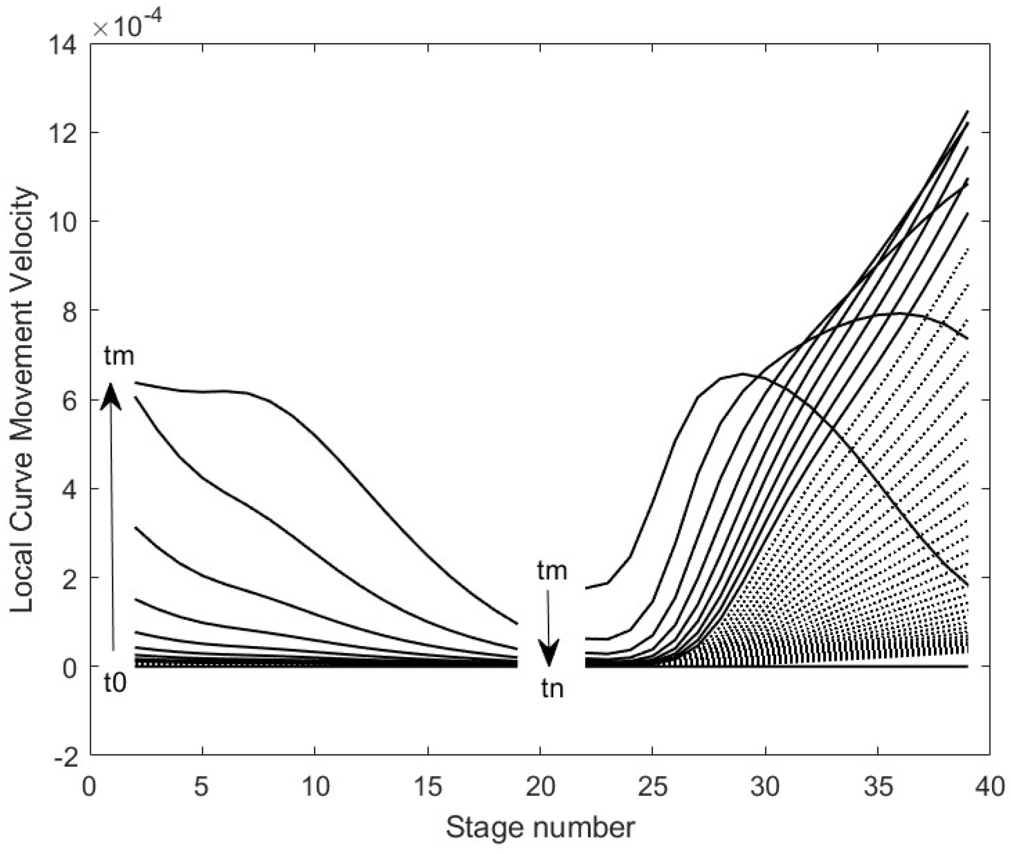
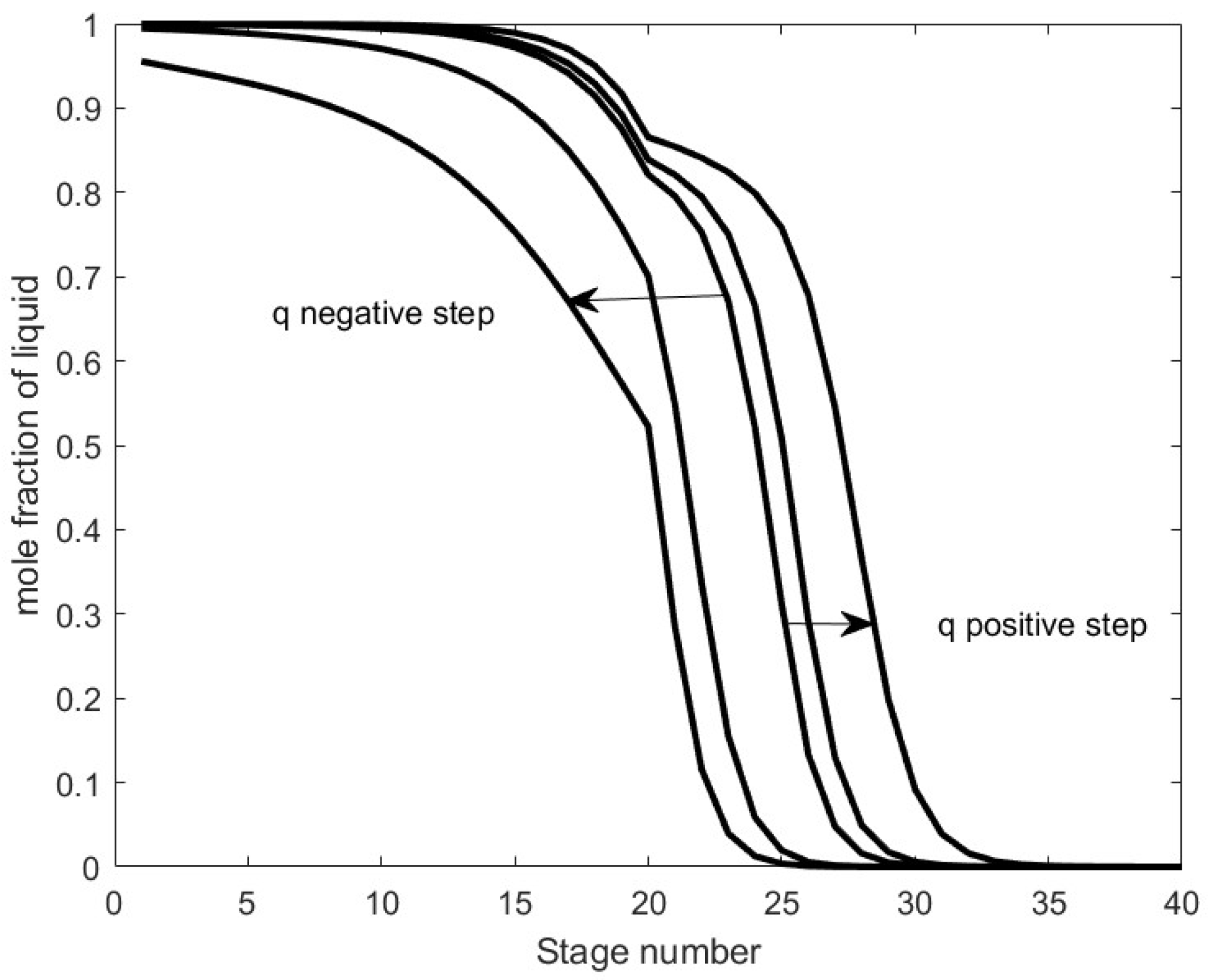
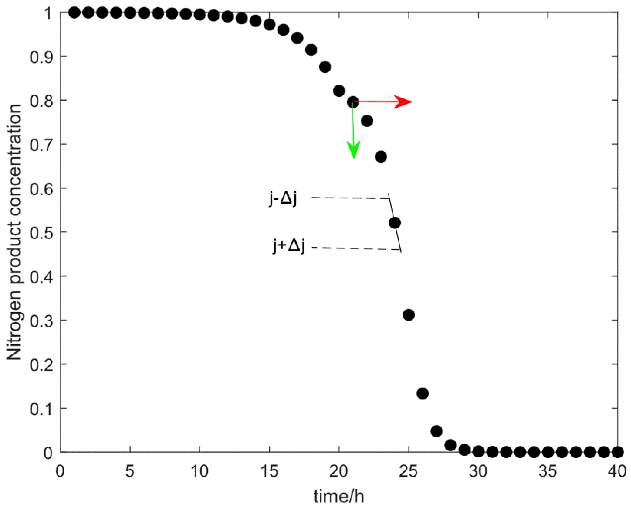
As illustrated in Figure 6, during most dynamic processes, the local movement velocities of the component concentration waveforms around individual trays vary, resulting in a time-varying spatial structure of the waveforms. To accurately capture these variations, the following method is adopted to evaluate the degree of local waveform distortion:

(1) Assume the first sampling instant of the current loop is $k$, let ${\tau }_0=k$, which is recorded as the initial moment for the accumulation of local waveform distortion degree;

(2) Calculate the local wave velocity (${\displaystyle \frac{d{s}_i{\mid }_{j-\Delta j}^{j+\Delta j}}{dt}}$) of all trays at the current moment according to Equation (33);

(3) Use the Euler method to calculate the movement distance of the local waveform:

$$\left\{\begin{array}{c}{S}_{i,j}^k={\displaystyle \frac{d{S}_i^k{|}_{j-\Delta j}^{j+\Delta j}}{dt}},k={\tau }_0\\ S_{i,j}^k=S_{i,j}^{k-1}+{\displaystyle \frac{d{S}_i^k{|}_{j-\Delta j}^{j+\Delta j}}{dt}}\Delta t,k>{\tau }_0\end{array}\right.$$

(34)

where ${\tau }_0$ is the initial moment for the accumulation of local waveform movement distance, $\Delta t$ represents the time interval, and $S_{i,j}^k$ represents the accumulated amount of local waveform displacement for each component concentration starting from the initial moment ${\tau }_0$.

(4) Calculate the average value of the displacement accumulation ${\overline{S}}_{i,j}^k$, and use the standard deviation ${\sigma }_i^k$ to represent the distortion degree of the component concentration waveform, that is:

$${\sigma }_i^k=\sqrt{{\displaystyle \frac{1}{k-{\tau }_0}}{\displaystyle \sum _{\tau ={\tau }_0}^k}{(S_{i,j}^k-{\overline{S}}_{i,j}^k)}^2}$$

(35)

(5) Define the boundary value $d$ for the local deviation degree of the component concentration waveform, which is used to evaluate whether the local deformation degree of the component concentration waveform exceeds the acceptable range. If ${\sigma }_i^k<d$, it indicates that the local deformation degree of the concentration waveform is within the acceptable range. At the next sampling instant $k=k+1$, the calculation starts from step (2), and the value of ${\tau }_0$ remains unchanged; if ${\sigma }_i^k>d$, it indicates that the local deformation degree of the concentration waveform exceeds the acceptable range, and the model needs to be updated at this time. Then, starting from step (1), recalculate ${\sigma }_i^k$, and the value of ${\tau }_0$ at this time will be reset.

When the structure of the component concentration curve of the entire column changes, the smaller $S_{i,j}^k$ is, the smaller the local deformation degree of the concentration waveform; the larger $S_{i,j}^k$ is, the larger the local deformation degree of the concentration waveform. The decision on whether to update the model is determined by the value of ${\sigma }_i^k$. Based on the above content, a model update method based on the local deviation degree of the component concentration waveform is proposed, that is, updating the model when ${\sigma }_i^k>d$.

4.2. Development of Nonlinear Optimization Models with Parameter Updating

It is worth noting that in closed-loop simulation experiments, when the system approaches a steady state, the waveform of the component concentration fluctuates within a very small range. This results in ${\sigma }_i^k$ remaining consistently smaller than $d$, preventing the triggering of model updates and leading to continuous error accumulation. Therefore, relying solely on a single criterion for parameter updates may be unreasonable. To address this issue, we investigate and comparatively study the following four adaptive model parameter update methods:

(1) Update model parameters in real-time at every sampling instant;

(2) Adopt equidistant sampling, updating the model parameters once every 20 sampling times;

(3) Update the model parameters once when ${\sigma }_i^k>d$ ($d=5\times 10^{-5}$);

(4) Update the model parameters once either when ${\sigma }_i^k>d$ ($d=5\times 10^{-5}$) or every 20 sampling times.

Applying these four optimization methods to the nonlinear wave model of the HIASC yields four distinct nonlinear optimization models based on parameter updating. Once the models are established, dynamic testing is required to verify their effectiveness. The solution procedure for the models follows the steps below:

(1) Identify the waveform parameters $X_{i,r\_max}$, $X_{i,r\_min}$, $k_r$, $X_{i,s\_max}$, $X_{i,s\_min}$, $k_s$ and the initial inflection point positions $S_r$, $S_s$ under initial steady-state conditions.

(2) Calculate the moving velocity of each component concentration curve according to the wave velocity Formulas (18) and (19).

(3) Calculate the inflection point positions $S_r$ and $S_s$ at the next time step using the Euler method:

$$S_r^{k+1}=S_r^k+{\displaystyle \frac{d{S}_r}{dt}}\cdot \Delta t$$

(36)

$$S_s^{k+1}=S_s^k+{\displaystyle \frac{d{S}_s}{dt}}\cdot \Delta t$$

(37)

(4) Solve Equations (11) and (12) to obtain the observed concentration values ${\widehat{X}}_{i,j}$ at each tray at the next time step.

(5) Select an optimization method to update the model parameters $X_{i,r\_max}$, $X_{i,r\_min}$, $k_r$, $X_{i,s\_max}$, $X_{i,s\_min}$, $k_s$.

(6) Return to step (2) and proceed to the next sampling instant by setting $k=k+1$, until the simulation time ends.

4.3. Dynamic Testing of the Model

The initial conditions are shown in

Table 1. The initial operating conditions of the HIASC.

Operation Condition	Value	Operation Condition	Value
Feed Flow Rate F (kmol/s)	128.1	Feed Components N2, Ar, O2	0.78118, 0.00932, 0.2095
Feed Temperature Tf (K)	101.3	Holdup H (kmol)	1
Feed Tray f	20	Pressure of Rectifying Section Pr (Pa)	579,573
Number of Trays n	40	Pressure of Stripping Section Ps (Pa)	115,718
Feed Thermal Condition q	0.26	Side Draw Tray	25

. Based on the initial conditions, step changes are applied to the operating conditions, and the established nonlinear optimization model based on parameter updating is evaluated in terms of accuracy and operational efficiency. Subsequently, the pros and cons of the aforementioned optimization methods are comprehensively assessed through the operation results. For convenience of description, the operation curve of the mechanism model [16,17] is denoted as “real concentration”; the optimization method updated every 20 sampling times is denoted as “updating by 20 moments”; the optimization method when ${\sigma }_i^k>d$ ($d=5\times 10^{-5}$) is denoted as “updating with $\sigma >d$ “; and the optimization method when ${\sigma }_i^k>d$ ($d=5\times 10^{-5}$) or every 20 sampling times is denoted as “updating with composite method”.

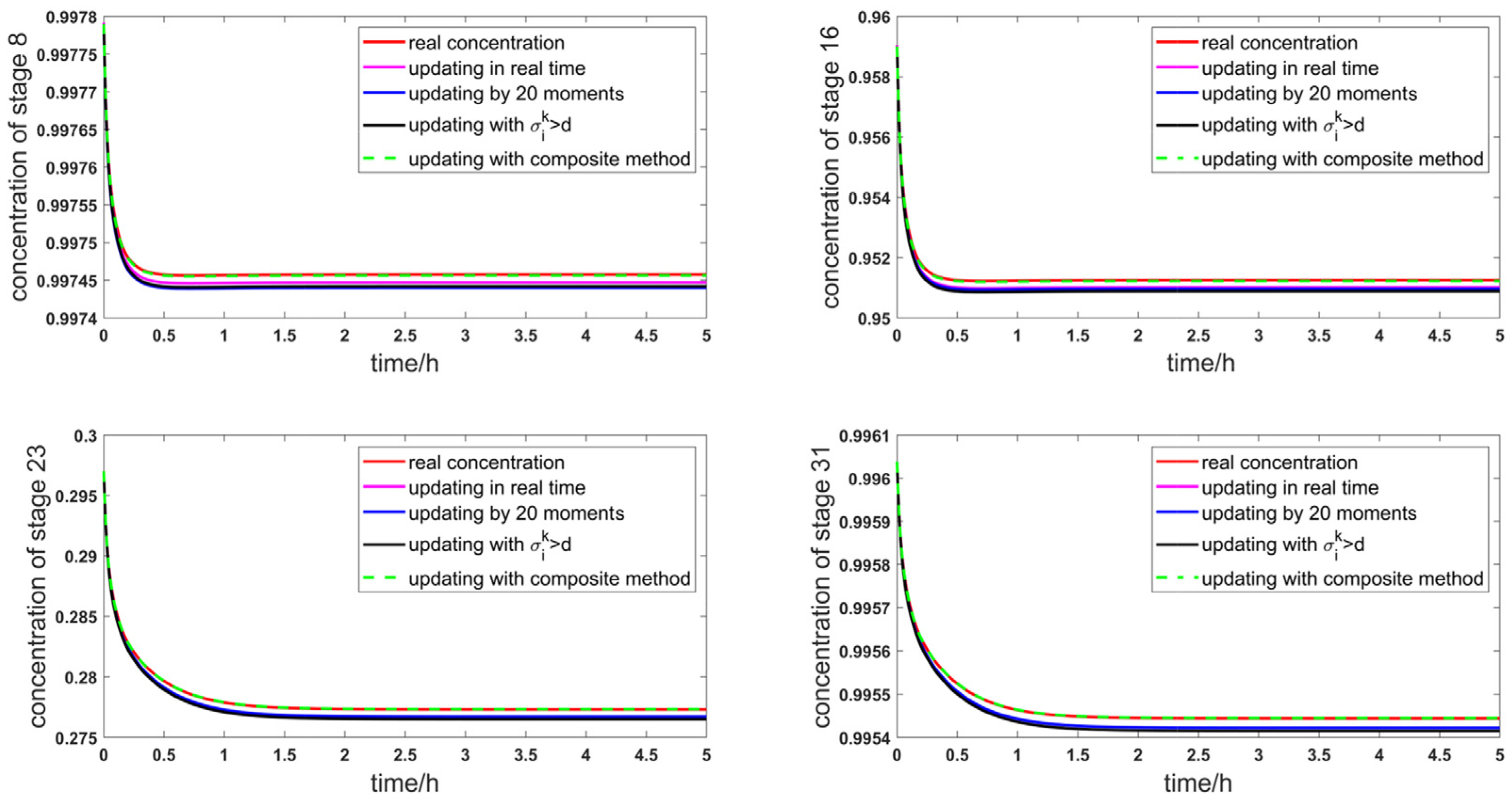
Figure 7 illustrates the dynamic tracking performance of various models for the component concentrations at trays 8, 16, 23, and 31 under different updating methods when the feed flow rate $F$ increases by 10%. As can be seen from the figure, a 10% increase in $F$ leads to certain tracking errors for the middle trays across the different updating methods. Specifically, when the system reaches a steady state, there is a noticeable steady-state error between the observed and real values. However, throughout the entire dynamic response process, all the models are capable of accurately reflecting the variation trends of the concentrations.

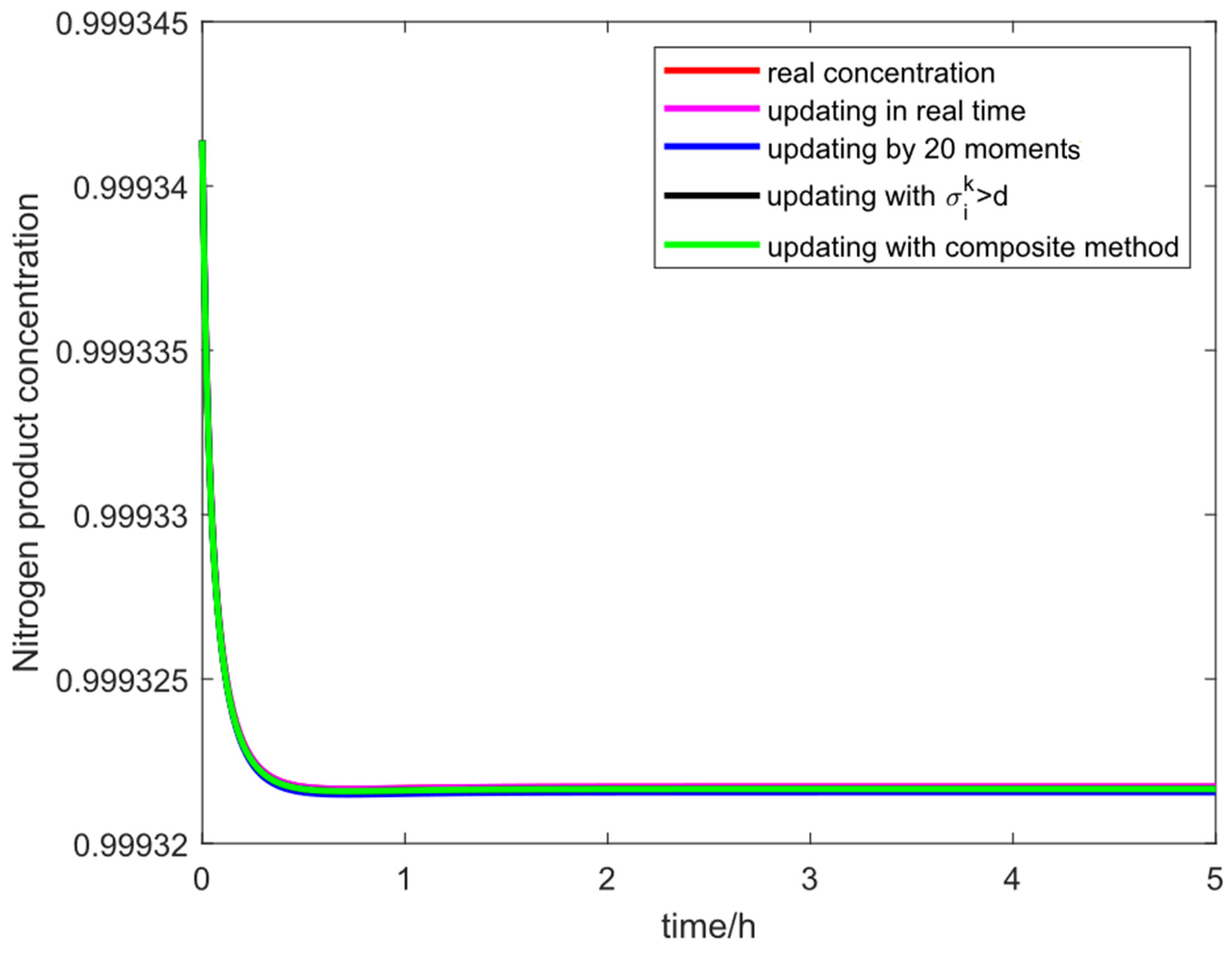
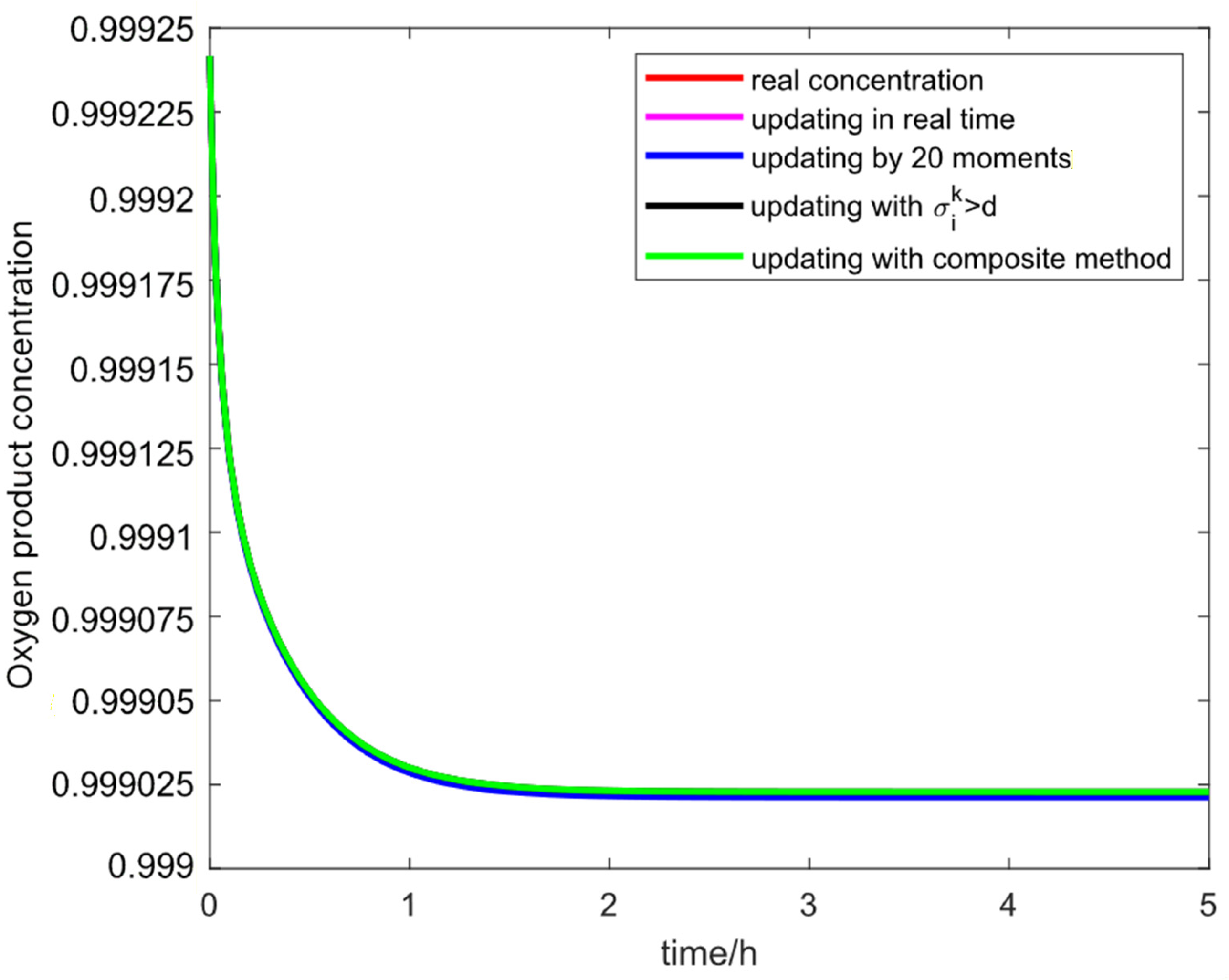
Figure 8 and Figure 9 illustrate the dynamic tracking performance of the models for the top and bottom product concentrations under different updating methods when the feed flow rate $F$ increases by 10%. As observed, the dynamic tracking curves of the models under various updating methods basically coincide with the observation curves of the mechanistic model. This indicates that the observed concentrations are highly consistent with the true concentrations, demonstrating excellent observation accuracy. It should be noted that during the model identification process, the optimization weights are biased towards the accuracy of the top and bottom products. Consequently, the concentration errors at the top and bottom are relatively small, whereas those at the middle trays are larger. The primary reason is that, from the perspectives of both product quality monitoring and subsequent online real-time control, the concentrations of the products at both ends are more critical variables, thus requiring higher observation accuracy.

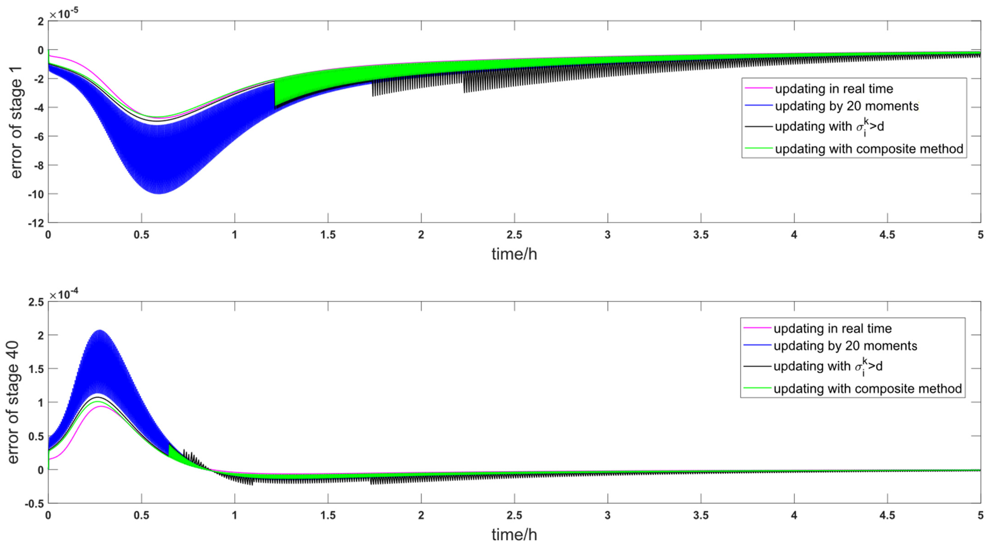
To clearly demonstrate the differences in concentration tracking errors of the products at both ends under different methods, we plotted the error values from Figure 8 and Figure 9 separately. This was done by subtracting the baseline values of the mechanistic model from the concentration values obtained by the four models, as shown in Figure 10.

Observation reveals that when updating model parameters every 20 sampling times, the concentration tracking error exhibits severe oscillations in the early stage of the dynamic response. It takes a long time to converge to zero, and a dynamic tracking error for the bottom product concentration persists. When updating model parameters using the condition ${\sigma }_i^k>d$, the concentration tracking error oscillates after the system reaches a steady state, particularly in the top section of the column. However, the composite update method combines the advantages of these two methods, resulting in very small tracking errors throughout the entire dynamic response process, with virtually no steady-state error.

Subsequently, the computational efficiency of the model under different updating methods is analyzed. The dynamic response time is set to 5 h, and 16,000 sampling points are extracted during the simulation to represent the real-time response. To objectively evaluate the computational efficiency and reduce the random errors generated during a single run, all the simulation times reported in this paper are calculated as the average values obtained from 50 consecutive runs of the program. This metric serves as the core indicator for evaluating computational efficiency.

Table 2. Number of updates and runtime under different update methods when $F$ increases by 10%.

Update Method	High-Pressure Column Update Count	Low-Pressure Column Update Count	Runtime/Second
Real-time update	16,000	16,000	206.81
Every 20 moments	800	800	26.92
σik > d	472	3979	42.03
Composite method	1170	4179	43.21

presents the number of updates and the runtime for the high-pressure and low-pressure columns under different updating methods during the dynamic response process when the feed flow rate $F$ increases by 10%. As can be seen from the table, the real-time update method requires the longest runtime, indicating a high frequency of model parameter updates but also resulting in an excessively high computational burden. Conversely, the method of updating every 20 sampling times has the shortest runtime. While this reduces the computational load due to its low update frequency, it is evident that the updates are insufficiently timely, leading to larger errors.

In contrast, the methods of updating model parameters when ${\sigma }_i^k>d$ and the composite update method not only significantly reduce the number of updates but also substantially improve the computational efficiency. This is primarily because the selection of sampling instants in these two methods is based on the intrinsic characteristics of the HIASC. Consequently, the sampling settings are more rational, effectively balancing model accuracy and computational efficiency. Furthermore, since the composite update method yields higher model accuracy and smaller errors, it achieves the best overall performance.

5. Conclusions

This paper proposes a nonlinear wave model based on model updating for the internally heat-integrated air separation column (HIASC). For such a complex HIASC system, the assumptions of constant wave velocity and constant molar overflow are no longer applicable. Therefore, the model parameters must be time-varying to accurately describe the dynamic process of concentration changes and to observe the product concentrations at both the top and bottom of the column. Since these model parameters cannot be measured directly, they must be estimated online, which inevitably incurs a high computational cost. Based on local mechanistic analysis of the HIASC concentration profiles, this paper proposes a model updating strategy based on the degree of concentration wave distortion.

Traditional wave theory focuses on the overall movement of concentration waves, which fails to accurately describe their local variations. To address this, this paper introduces the concept of distributed wave velocity to conduct a local analysis of the concentration waveform, thereby obtaining the displacement of the waveform at each tray over a given period. By studying the discrete boundaries of the displacement, the local waveform distortion degree is evaluated to determine whether the model parameters need to be updated. This approach effectively balances model accuracy and computational efficiency, thereby reducing the computational cost.

The proposed evaluation method is incorporated into the wave model, and four updating strategies are proposed and tested via simulation. The simulation results indicate that a fixed update frequency causes severe oscillations in the initial stage of disturbance, leading to poor concentration observation performance. Conversely, a single displacement discrete boundary condition produces significant oscillations as the system approaches a steady state. Although the real-time updating strategy yields the smallest error, it incurs the highest computational cost. Ultimately, the composite updating strategy demonstrates significant advantages in comprehensively balancing model simplification, observation accuracy, and operational efficiency.