1. Introduction
The Job Shop Scheduling Problem (JSSP) concerns the assignment and sequencing of operations on shared machines while satisfying technological precedence and machine-capacity constraints [
1,
2,
3]. Minimising the makespan is one of the most widely studied objectives in JSSP optimisation. Due to its combinatorial nature, the deterministic JSSP is NP-hard, and the construction of effective machine-order representations remains a fundamental issue in both exact and approximate scheduling methods. In practice, processing times are rarely known exactly, and reliable probability distributions are often unavailable, but lower and upper duration bounds can usually be estimated effectively. The Interval Job Shop Problem (IJSP) therefore models processing-time uncertainty by representing each operation duration as an interval defined by its lower and upper bounds [
4]. Unlike formulations that rely on explicit probability distributions, such as chance-constrained scheduling [
5], the IJSP can therefore represent processing-time uncertainty using only these interval bounds.
Most IJSP methods adopt a sequence-first strategy in which a complete operation or machine sequence is determined before interval durations are propagated for evaluation [
6,
7,
8]. Robust scheduling research, by contrast, indicates that retaining selected sequencing freedom can support adaptability under uncertain durations [
9,
10,
11]. This contrast motivates a representation that fixes sufficiently stable machine conflicts while deferring timing-sensitive relations to execution.
The key challenge is therefore to determine which machine conflicts should be committed before execution and which should remain open. Resolving all same-machine relations removes potentially useful temporal flexibility, whereas retaining too many leaves an unnecessarily large residual decision space. The resulting problem is to balance combinatorial reduction against flexibility under interval uncertainty.
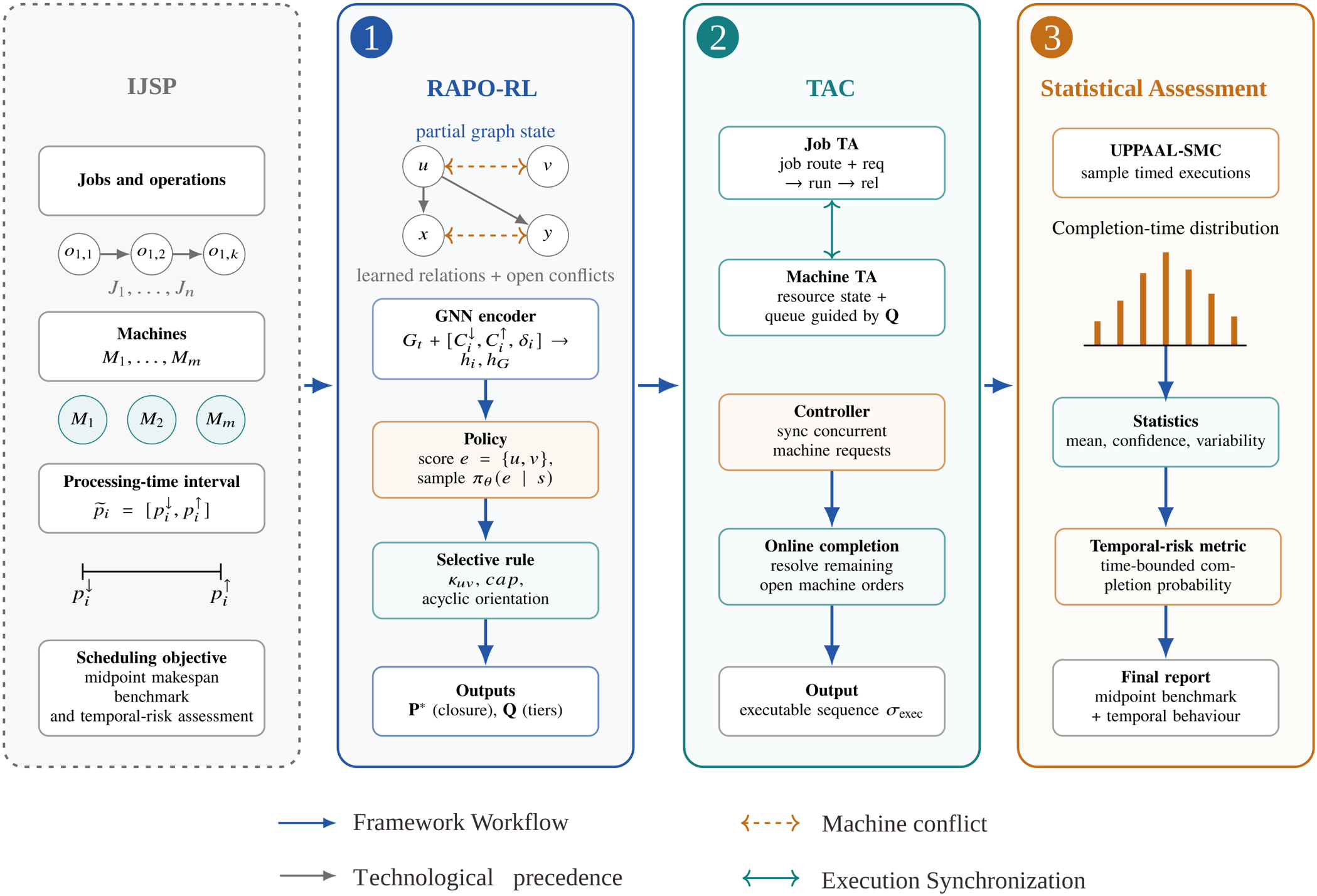
To address this problem, we propose Risk-Aware Partial-Order Reinforcement Learning with Timed Automata Completion (RAPO-RL-TAC). Its learning component, Risk-Aware Partial-Order Reinforcement Learning (RAPO-RL), constructs a machine partial order by resolving comparatively stable conflicts while retaining a bounded number of timing-sensitive relations. Timed Automata Completion (TAC) subsequently resolves the deferred relations as execution evolves, after which statistical model checking characterises completion-time distributions and temporal variability.
The main contributions are as follows:
- 1.
Reinforcement learning for partial-order construction in the IJSP. Rather than learning a complete machine sequence, RAPO-RL learns which machine-conflict relations should be committed before execution, prioritising conflicts that are comparatively less sensitive to interval uncertainty while retaining temporally ambiguous relations for later resolution. The resulting directed partial order eliminates a substantial portion of the combinatorial ambiguity before formal temporal analysis, thereby reducing the residual branching space and improving the tractability of model-checking-based scheduling for the IJSP.
- 2.
A risk-aware selective commitment algorithm under interval uncertainty. We introduce a risk-aware selective-commitment mechanism that explicitly accounts for interval-induced ordering uncertainty when determining which machine conflicts should be fixed before execution. A temporal-determinacy criterion characterises each unresolved conflict using interval-derived execution-window overlap and ordering criticality, while a machine-wise open-edge budget limits the number of deferred relations. By committing comparatively stable conflicts and retaining timing-sensitive conflicts whose ordering is more susceptible to processing-time realisations, the risk-aware mechanism avoids premature commitment and preserves temporal flexibility while controlling the residual decision space.
- 3.
A timed-automata completion framework for the IJSP. We formulate residual machine-order uncertainty and interval processing times within a timed-automata model in which unresolved sequencing relations are completed according to the evolving temporal state. This formulation connects the learned partial order to executable schedules without requiring all machine orders to be fixed in advance; statistical model checking is then used to sample timed executions and characterise completion-time distributions and variability under interval uncertainty.
The remainder of the paper is organised as follows.
Section 2 provides a comprehensive review of the related work.
Section 3 defines the IJSP and presents the overall RAPO-RL-TAC framework.
Section 4 details the reinforcement learning for partial-order construction and the risk-aware selective commitment algorithm, and
Section 5 presents the method of timed automata completion and statistical temporal assessment.
Section 6 reports the benchmark, ablation, and statistical-model-checking experiments.
Section 7 concludes the paper.
2. Related Work
Existing studies relevant to solving job-shop problems under interval or other processing-time uncertainty can be organised into four methodological directions: metaheuristic optimisation, machine-learning-based scheduling, formal methods for JSSP scheduling, and hybrid methods. Metaheuristic optimisation constructs schedules under uncertain durations using neighbourhood, evolutionary, and swarm-intelligence approaches, with robustness-oriented criteria adopted where appropriate to evaluate uncertainty sensitivity; machine-learning-based scheduling learns scheduling or dispatching decisions from structured shop states; formal methods for JSSP scheduling use state-transition models and verification techniques to represent and analyse temporal scheduling behaviour; and hybrid methods combine data-driven decision making with explicit formal or event-based models. Representative foundations include interval and robustness-oriented optimisation methods [
12,
13], graph- and reinforcement-learning-based schedulers [
14,
15,
16,
17], robustness-evaluation methodology [
18], and broader JSSP taxonomies [
19]. This organisation classifies the literature by solution mechanism rather than using the IJSP itself as a research-direction label.
2.1. Metaheuristic Optimisation Under Processing-Time Uncertainty
Metaheuristic optimisation is a principal line of work for the IJSP because interval-valued processing times can be incorporated directly into schedule evaluation. Lei [
6] developed population-based neighbourhood search (PNS) using an ordered operation-based representation and interval-makespan evaluation. Díaz et al. [
7] subsequently proposed a genetic algorithm (GA) in which candidate sequences are decoded and evaluated under interval uncertainty. Artificial-bee-colony and neighbourhood-search variants have also been developed for interval job shops with flexible maintenance, dual-resource and environmental constraints, and makespan objectives [
12,
20,
21,
22]. Díaz et al. [
8] later proposed the Fast Elitist Artificial Bee Colony (fEABC) algorithm, simplifying the underlying artificial bee colony structure to reduce runtime while retaining competitive interval-makespan performance. Afşar et al. [
23] extended interval-based optimisation to a green flexible job-shop setting through a hybrid evolutionary approach with lexicographic production and environmental objectives.
Complementary uncertainty-aware studies evaluate robustness and risk rather than only a nominal interval makespan. Beck and Wilson [
24] studied proactive job-shop scheduling with probabilistic activity durations. Wang et al. [
25] formulated bad-scenario-set robust job-shop scheduling under processing-time uncertainty and solved it with tabu search. For interval-valued blocking job shops, Meloni et al. [
26] evaluated makespan risk using value-at-risk and conditional value-at-risk. Calamita et al. [
27] subsequently used machine learning to accelerate such risk estimation, while Himmiche et al. [
18] presented a broader robustness-evaluation process for schedules under uncertainty.
A related robustness-oriented line preserves sequencing flexibility instead of fixing every resource order in advance. Earlier work studied graph-based decomposition, solution flexibility, and partial-order schedules as mechanisms for retaining alternatives under perturbations [
9,
10,
28,
29]. Rivière et al. [
11] proposed a two-stage stochastic/robust method based on permutable operation groups, allowing part of the sequencing decision to be deferred until uncertainty is realised. Ourari et al. [
30] more recently developed a robust job-shop scheduling approach based on sequential flexibility, retaining alternative machine sequences that can be adapted when disturbances occur during execution.
Taken together, these studies establish metaheuristic optimisation, explicit robustness/risk evaluation, and delayed sequencing as complementary responses to processing-time uncertainty. Most direct IJSP optimisers nevertheless return a complete sequence before temporal execution, whereas flexibility-oriented robust methods preserve alternatives without learning which individual machine conflicts should remain unresolved. This distinction motivates the selective partial-order representation used in RAPO-RL-TAC.
2.2. Machine-Learning-Based Scheduling
Machine-learning-based scheduling increasingly uses learned policies to construct job-shop decisions from structured shop states. Zhang et al. [
14] introduced Learning to Dispatch, representing the evolving JSSP as a disjunctive graph and using a graph neural network (GNN) with Proximal Policy Optimisation (PPO) to learn priority dispatching rules. Park et al. [
15] combined graph neural networks with reinforcement learning for joint representation and policy learning, and demonstrated transfer to previously unseen JSSP instances. Broader methodological perspectives on machine learning for combinatorial optimisation and the reliability of reinforcement-learning-based production scheduling are provided by Bengio et al. [
31] and Waubert de Puiseau et al. [
32], respectively. Cai et al. [
33] and Yang et al. [
34] further illustrate deep-reinforcement-learning and graph-based approaches in static and dynamic job-shop settings.
Uncertain processing times have also been incorporated directly into learned scheduling policies. Wu et al. [
16] formulated dynamic job-shop scheduling with uncertain processing times as a reinforcement-learning problem using priority-rule actions and policy reuse under changing durations. Infantes et al. [
17] addressed JSSP scheduling with uncertain activity durations and used deep reinforcement learning to search for robust schedules while studying generalisation and scalability. These studies show that uncertainty can enter the learning process itself rather than being considered only after a complete deterministic schedule has been generated.
Recent surveys reinforce this methodological trend. Lv et al. [
35] review deep-reinforcement-learning approaches to job-shop scheduling, Smit et al. [
36] focus on graph neural networks for JSSP, and Xu et al. [
37] survey learning-to-optimise methods with comparisons between genetic programming and reinforcement learning. Meilanitasari and Shin [
38] provide a complementary review of prediction and optimisation for sequence-driven scheduling in job-shop flexible manufacturing systems.
Despite differences in state representation and learning architecture, these methods generally use learning to select dispatching actions, operations, or progressively complete a schedule. Comparatively less attention has been paid to policies that deliberately return an incomplete machine-order representation in which only selected conflict relations are committed and the remaining relations are transferred to a separate temporal-completion stage.
2.3. Formal Methods for JSSP Scheduling
Formal methods provide mathematically defined state-transition models for expressing timing, synchronisation, and resource constraints. Timed automata extend finite-state models with real-valued clocks [
39]; tool-supported timed-automata analysis and simulation-based statistical model checking (SMC) provide practical mechanisms for reachability analysis, temporal-property checking, and statistical estimation [
40,
41]. At this methodological level, the emphasis is on the formal modelling and analysis paradigm rather than on any particular software implementation.
Formal temporal models have been applied directly to scheduling and robustness analysis. Behrmann et al. [
42] formulated production scheduling as reachability analysis over timed-automata models. Malik and Pena [
43] used model checking to compute time-optimal task schedules in a flexible manufacturing system. Bendík et al. [
44] analysed the robustness of timed automata under perturbations of timing constants using model-checking techniques. In production scheduling under uncertainty, Himmiche et al. [
18] evaluated how uncertain temporal behaviour affects schedule robustness.
Formal and statistical analysis can also characterise distributional or service-level performance beyond a single nominal makespan. Meloni and Pranzo [
45] studied makespan quantiles and superquantiles in interval-valued activity networks. Flores-Gómez and Dauzère-Pérès [
46] formulated a makespan service-level criterion for flexible job-shop scheduling under machine-related uncertainty, evaluating the probability that makespan remains below a specified threshold.
Existing formal approaches therefore support schedule synthesis, temporal-property verification, robustness analysis, and statistical evaluation of uncertain execution. In most cases, scheduling decisions are generated inside the formal model or supplied as a substantially specified scheduling structure. The use of a learned partial machine order as an intermediate representation for subsequent formal completion remains comparatively underexplored.
2.4. Hybrid Methods
Hybrid methods combine data-driven decision making with explicit formal, logical, or event-based structure. Lassoued and Schwung [
47] proposed PetriRL, which integrates Petri nets with event-based deep reinforcement learning for JSSP optimisation: the Petri-net model represents the production process and constraints, while reinforcement learning operates at decision points in the event-driven environment. This provides an example in which the formal/event model is part of the scheduling environment itself.
A complementary pattern appears in safe reinforcement learning. Hamel-De le Court et al. [
48] proposed probabilistic shielding, in which formally derived safety information is used to restrict actions that could violate a probabilistic safety requirement. Although this work is not a job-shop scheduling method, it is relevant as evidence that formal analysis can constrain a learned policy rather than merely evaluate its output.
These studies illustrate two representative hybridisation patterns: structured models can define the environment in which learning operates, and formal analysis can restrict the action space of a learned policy. By comparison, reinforcement-learning-based schedulers generally generate decisions directly [
14,
15,
16,
17], whereas model-checking-based scheduling approaches perform synthesis or temporal analysis within the formal model [
42,
43]. RAPO-RL-TAC occupies an intermediate position: learning first reduces the machine-order decision space, and a subsequent formal temporal model completes the deliberately retained relations.
Table 1 summarises representative studies across the four methodological directions.
4. Risk-Aware Partial-Order Reinforcement Learning (RAPO-RL)
RAPO-RL is designed to reduce the machine-order decision space before timed execution while preserving a limited number of relations that are strongly affected by interval uncertainty. Starting from the disjunctive-graph representation of an IJSP instance, the method progressively converts selected machine-conflict edges into directed precedence relations. A GNN encodes the evolving partial graph, and a reinforcement-learning policy uses the learned graph representation to determine which unresolved conflict should be processed next. Temporal determinacy and an open-edge budget control which relations are committed during learning and which are retained for subsequent timed-automata completion.
In RAPO-RL, risk awareness refers to explicit sensitivity to interval-induced temporal uncertainty when machine-order relations are committed. The implementation follows three connected stages in this section. First, the risk-aware determinacy assessment in
Section 4.3 quantifies the ordering uncertainty of unresolved machine conflicts. Second, the open-edge budget in
Section 4.4 retains a controlled number of low-determinacy relations for later completion. Third, the reward design in
Section 4.5 incorporates pessimistic residual uncertainty, processing-time interval width, and perturbation sensitivity into policy learning. Together, these mechanisms discourage premature commitment while preserving a bounded degree of temporal flexibility.
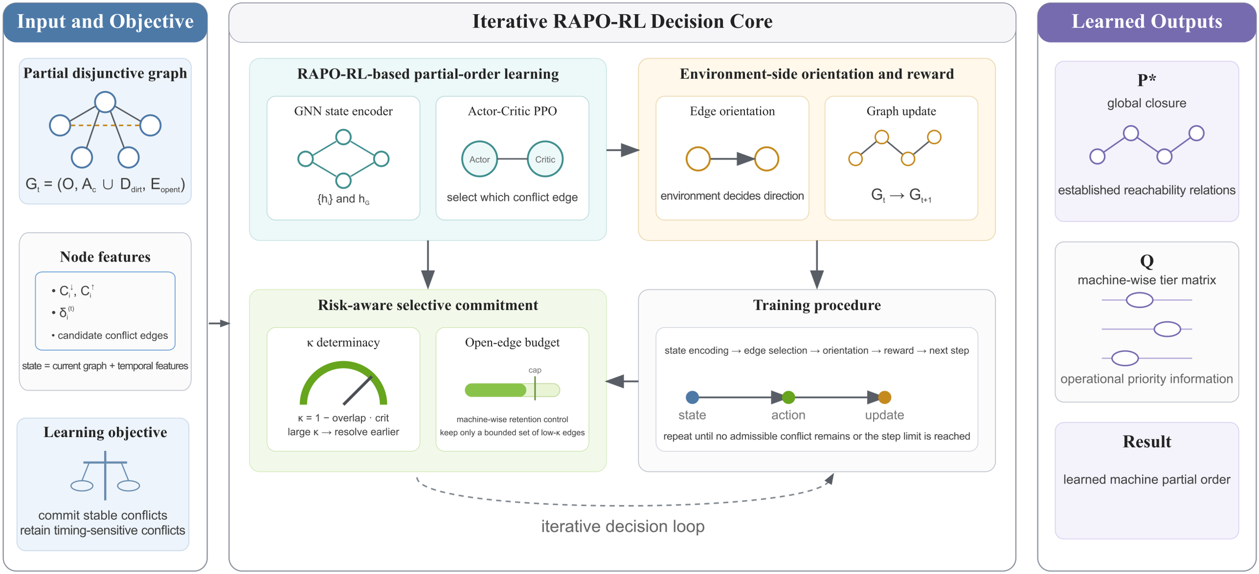
The learning policy does not directly determine the orientation of a selected edge. Instead, it learns a global priority over unresolved machine conflicts, while the environment determines the direction of the selected relation using temporal information and acyclicity-preserving rules. This separation allows the GNN and reinforcement-learning policy to focus on identifying informative conflict-resolution decisions without expanding the action space to all possible edge-direction combinations.
Figure 2 provides an overview of this learning-and-resolution workflow and the two learned output representations used by the subsequent completion stage.
4.1. Disjunctive Graph and Partial Disjunctive Graph Representation
An unresolved IJSP instance is represented by a mixed disjunctive graph , where is the operation set, contains the directed technological-precedence arcs, and contains the undirected conflict edges between operations requiring the same machine. Each edge therefore represents a machine-order relation that has not yet been determined.
During RAPO-RL, selected conflict edges are progressively oriented. At decision step
t, the current partial disjunctive graph is represented as
where
is the set of machine-conflict relations already oriented at step
t, and
is the set of unresolved machine-conflict edges. Initially,
and
. Unlike complete-sequence construction,
is allowed to remain non-empty at termination because selected timing-sensitive relations are deliberately retained for the downstream completion stage.
The directed part of
, consisting of technological arcs and currently established machine-precedence relations, provides the structural input to the GNN. Open conflict edges are maintained separately as candidate decisions rather than being inserted into the message-passing adjacency structure. This avoids propagating messages through dense unresolved machine-conflict cliques and allows the encoded graph to represent only precedence information that has already been established [
14].
Because
is generally incomplete, it does not define a unique executable schedule. Instead, lower and upper completion-time estimates are propagated along the currently established directed relations:
where
and
are the lower and upper completion estimates of operation
, respectively;
and
are its processing-time bounds; and
is the set of currently established predecessors of
. The maximum is taken as zero when
. These quantities do not represent the final makespan; they provide temporal features for evaluating and learning from the evolving partial order.
4.2. RAPO-RL-Based Partial-Order Learning
The partial-order construction process is formulated as a sequential decision problem. At each decision step, RAPO-RL receives the current partial disjunctive graph, encodes its structural and temporal state using a GNN, evaluates the currently admissible machine-conflict edges, and selects one edge for resolution. The environment subsequently determines its direction and updates the graph. Repeating this interaction gradually converts the unresolved disjunctive graph into a machine partial order.
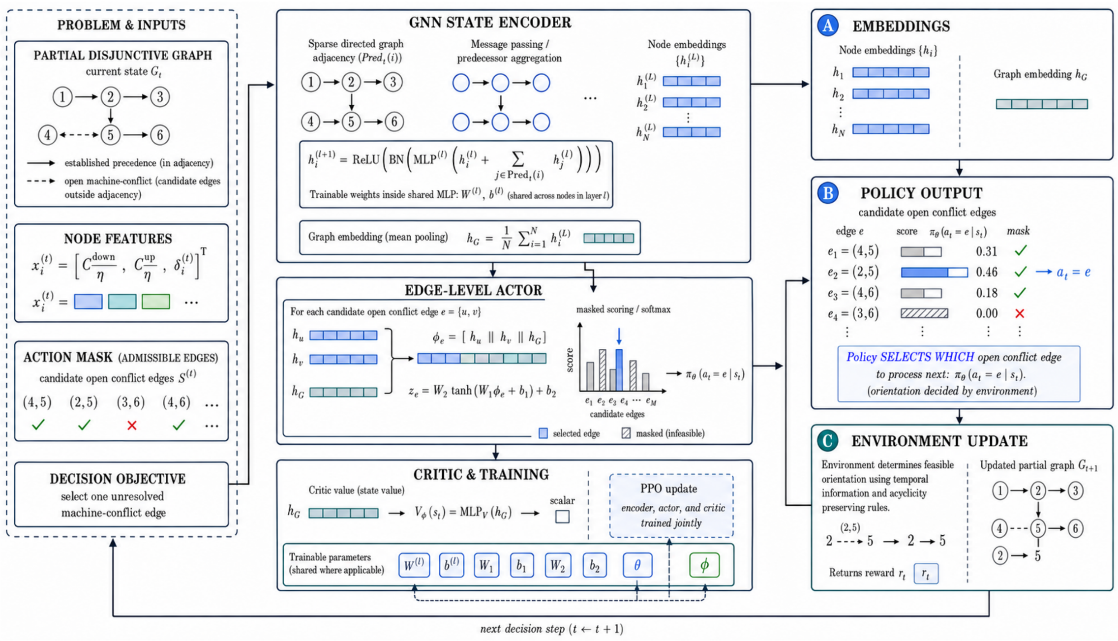
The information flow is therefore: partial disjunctive graph and node features → GNN state encoder → node and graph embeddings → edge-level actor policy → selected open conflict edge → environment update → updated partial graph.
Figure 3 illustrates how the scheduling state is converted from graph and node-feature inputs into learned embeddings, edge-selection probabilities, and the next partial-graph state.
4.2.1. Markov Decision Process
The partial-order construction process is modelled as a Markov decision process
[
14]. At decision step
t, the state
contains the current partial graph together with its temporal and structural features. An action selects one currently admissible machine-conflict edge for processing. Importantly, the action identifies which conflict should be resolved; it does not specify whether
or
should be introduced. That direction is determined by the environment after the edge has been selected. The transition to
therefore reflects both the learned edge choice and the environment-side orientation rule.
4.2.2. State Representation and Node Features
The GNN input combines the current directed precedence structure with interval-derived temporal information. Each operation
is represented by the node-feature vector
where
and
are the propagated lower and upper completion estimates,
is the time-normalisation constant, and
is the proportion of candidate same-machine conflict edges incident to
that have already been oriented. The first two components describe the current optimistic and pessimistic temporal position of the operation, while the third represents local progress in partial-order construction.
The GNN adjacency contains only established technological and machine-precedence relations. An incoming neighbour of therefore corresponds to an operation that is currently known to precede . Open machine-conflict edges remain outside the adjacency and are handled later by the edge-selection policy and its action mask.
4.2.3. GNN State Encoder
The purpose of the GNN is to transform the partially resolved scheduling graph into learned representations that capture both local operation relationships and the global state of the current partial order. The initial node embedding is
. Using sum aggregation, each message-passing layer applies a multilayer perceptron (MLP), batch normalisation (BN), and a rectified linear unit (ReLU) activation to update operation
as
where
is the embedding of operation
at layer
l,
is its predecessor set in the current directed graph, and
denotes the trainable MLP at layer
l. The trainable weight matrices and bias vectors inside the MLP are shared across operation nodes within the same layer and are learned jointly with the reinforcement-learning policy through PPO; they are not manually assigned scheduling weights.
After the final message-passing layer, the node embeddings are pooled into a graph-level representation:
where
N is the number of operations,
is the final embedding of operation
, and
summarises the overall partial-order state. Thus, the GNN produces operation-level embeddings for local conflict evaluation and a graph-level embedding for global context.
4.2.4. Edge-Level Actor Network
For each admissible unresolved machine-conflict edge
, the actor combines the embeddings of the two endpoint operations with the global graph representation. The edge representation and its policy score are defined by
where ‖ denotes vector concatenation;
,
,
, and
are trainable actor parameters; and
is the scalar score assigned to edge
e. The same actor weights are shared across all candidate edges, allowing conflicts from different machines and decision steps to be evaluated by one learned policy.
After prohibited edges are masked, the remaining scores are normalised into the edge-selection distribution
where
is the actor policy with parameters
,
is the current admissible-edge set, and
denotes selection of edge
e. The actor therefore answers the question: which unresolved machine conflict should be processed next, given the current partial-order state?
4.2.5. Critic Network
A critic network operates in parallel on the graph-level embedding and estimates the value of the current state, . The actor and critic share the GNN encoder but use separate output heads, so the encoder is trained to support both edge selection and state-value estimation. The critic is used only as the baseline required by actor–critic optimisation and does not introduce an additional scheduling decision.
4.2.6. PPO Policy Optimisation
The GNN encoder, actor, and critic are trained jointly using PPO [
14]. PPO updates the policy from collected trajectories while clipping excessively large policy changes between successive updates. Advantages are computed from the standardised trajectory returns and the critic baseline. The optimisation objective combines the clipped policy loss, value-function loss, and entropy regularisation, i.e.,
. Because PPO is used as the optimisation mechanism rather than as a new methodological contribution, the standard component losses are not expanded further here. This keeps the presentation focused on the scheduling-specific elements: graph-state encoding, edge prioritisation, selective commitment, and environment-side orientation.
4.3. Risk-Aware Determinacy Assessment for Selective Commitment
Risk-aware selective commitment in RAPO-RL begins by assessing the uncertainty associated with each unresolved machine conflict. Under interval processing times, the possible execution periods of two same-machine operations may overlap to different degrees, so some conflicts exhibit a comparatively stable ordering preference whereas others remain sensitive to the realised processing times. RAPO-RL quantifies this ordering uncertainty through a time-conflict determinacy score, which provides the primary criterion for deciding whether a conflict should be committed during learning or retained for later completion.
4.3.1. Estimated Execution Window
For each operation
, an estimated execution window is constructed from its current completion bounds:
where
is the estimated earliest start time,
is the pessimistic completion estimate,
and
are the propagated completion bounds, and
is the lower processing-time bound. The numerical window width is
.
4.3.2. Normalised Temporal Overlap
For an unresolved same-machine conflict
, the normalised overlap between the two estimated execution windows is
where
and
are the estimated start and completion limits of operations
u and
v, and
are their corresponding window widths. Values near zero indicate well-separated execution windows, whereas values near one indicate strong temporal overlap.
4.3.3. Ordering Criticality
Temporal overlap alone does not indicate how important the ordering choice is to the current schedule. We therefore compare the pessimistic local completion estimates associated with the two possible orders. Their normalised ordering criticality is
where
and
are the current pessimistic completion estimates,
and
are the corresponding upper processing-time bounds, and
is the current global pessimistic completion estimate.
4.3.4. Time-Conflict Determinacy Score
The final time-conflict determinacy score combines temporal overlap and ordering criticality:
where
measures the temporal overlap between the two operations and
measures the potential importance of their ordering. A larger
indicates a conflict whose ordering is comparatively more determinate under the current temporal approximation, whereas a smaller value identifies a more temporally ambiguous relation. Given the determinacy threshold
, conflicts with
are eligible for learning-stage resolution, whereas conflicts with
are treated as low-determinacy candidates for retention, subject to the machine-wise budget in
Section 4.4.
4.4. Open-Edge Budget Mechanism
The open-edge budget forms the second component of risk-aware selective commitment. A low determinacy score indicates that a relation may benefit from being resolved later during timed execution; however, retaining every such relation would leave an unnecessarily large residual decision space for the downstream timed-automata model. RAPO-RL therefore introduces a machine-wise open-edge budget.
For each machine, low-determinacy conflicts are ranked by
. When their number does not exceed the prescribed budget
, they are retained as open relations. If the number exceeds the budget, only the
conflicts with the smallest determinacy scores are retained; the remaining conflicts are returned to the admissible action set and must be processed by RAPO-RL. Consequently, the terminal partial order satisfies
where
is the set of low-determinacy conflicts remaining open on machine
at the end of learning,
is the maximum number of such relations allowed per machine, and
m is the number of machines. This mechanism creates an explicit trade-off between early conflict reduction and retained temporal flexibility: relations with relatively clear temporal structure are resolved before timed execution, while only a controlled number of the most temporally ambiguous relations remain open.
4.5. Environment-Side Orientation Rules and Reward Design
The reinforcement-learning policy determines which unresolved edge should be processed, whereas the environment determines the direction assigned to that edge. The environment also provides the reward used to train the policy. This separation keeps the learned action space compact while enforcing precedence consistency independently of the policy. The reward design further embeds risk awareness into policy learning by penalising decisions that increase pessimistic residual uncertainty or prematurely commit relations associated with wide processing-time intervals.
4.5.1. Local Edge Orientation Rules
To evaluate candidate orientations, the current partial graph is associated with the relaxed completion proxy
where
is the current partial graph and
are the propagated completion bounds of operation
. The quantity
is used only to rank local decisions and should not be interpreted as the realised or expected makespan of the completed schedule.
For a selected edge
, directions that would introduce a directed cycle are discarded. If the estimated execution windows are strictly separated, the temporally consistent acyclic direction is adopted directly. Otherwise, the environment selects
where
is the set of acyclic candidate directions for the selected edge and
is the direction producing the smallest relaxed completion proxy. This division allows the policy to focus on global edge prioritisation while the environment uses temporal structure and completion bounds for local orientation.
4.5.2. Pessimistic Reserve Metric
The immediate effect of an orientation is complemented by a pessimistic reserve that reflects the remaining uncertainty associated with unresolved conflicts:
where
denotes the current state,
is its maximum upper completion estimate,
is the unresolved conflict set, and the summation measures the difference between the two local pessimistic ordering estimates of each open conflict.
4.5.3. Step-Wise Reward
For the selected edge
, let
denote the combined processing-time interval width. The reward associated with an accepted conflict resolution is
where
is the reward for the transition from
to
,
and
are weighting coefficients,
is the pessimistic reserve, and
is the interval-width term defined above. The first term rewards improvement of the relaxed completion proxy, the second discourages decisions that increase residual pessimistic uncertainty, and the third discourages premature commitment of relations involving wide processing-time intervals.
4.5.4. Termination Robustness Reward
A terminal robustness term complements the step-wise reward by evaluating the learned partial order under sampled processing-time perturbations. Let
denote the makespan obtained using interval-midpoint processing times and let
be the corresponding makespan under Monte Carlo sample
k. The relative-deviation measure is
where
is the number of terminal Monte Carlo samples,
is the midpoint-based reference makespan, and
is the makespan obtained from sample
k. The terminal reward is
, where
controls the contribution of robustness to the learning signal. A smaller variation under processing-time perturbations therefore produces a larger terminal reward.
4.6. Training Procedure of RAPO-RL
Each RAPO-RL episode starts from the unresolved disjunctive graph of one IJSP instance and progressively constructs a partial order. At every decision step, the current completion bounds and node features are updated, the GNN generates node and graph embeddings, and the actor evaluates the admissible machine-conflict edges. After an edge is selected, the environment determines its orientation, updates the graph, and returns the corresponding reward. The next decision is therefore based on a newly encoded partial-order state.
Training is performed using multiple parallel environments and PPO updates. The GNN encoder, actor, and critic are trained jointly so that the learned graph representations become informative for edge-selection decisions. An episode terminates when no admissible conflict remains or the prescribed maximum number of decision steps is reached. Algorithm 1 summarises the complete training procedure.
| Algorithm 1 Compact pseudo-code of RAPO-RL partial-order learning and training. |
Input: , , , , , , PPO parameters .
Output: trained policy and instance-level outputs .
- 1:
Initialise encoder, actor, critic, and optimiser states. - 2:
for
do - 3:
Reset environments with . - 4:
while active environment exists do - 5:
Compute , node features , and determinacy scores . - 6:
Construct the action mask subject to and . - 7:
Encode and sample . - 8:
Apply and update . - 9:
Store . - 10:
If terminal, add with estimated from Monte Carlo completion samples. - 11:
end while - 12:
Compute standardised returns and advantages . - 13:
Update using the PPO objective defined in Section 4.2.6. - 14:
Every 100 iterations, evaluate the greedy policy and keep the best checkpoint. - 15:
end for - 16:
output and .
|
Algorithm 1 uses compact notation for the training loop. The input statement specifies the initial disjunctive graph , determinacy threshold , per-machine open-edge budget , maximum episode length , number of parallel environments , maximum number of PPO update iterations , and actor–critic parameters and . The set in Step 6 denotes the current conflicts protected from policy selection because they are retained by the low-determinacy rule and the machine-wise open-edge budget; is the indicator function, which equals 1 when its argument is true and 0 otherwise, so only conflicts outside remain selectable. The output statement records the trained policy together with the final directed and open conflict sets and the two instance-level representations and .
The numbered algorithm steps operate as follows. Step 1 initialises the shared GNN encoder, actor, critic, and optimiser states. Step 2 starts the outer PPO-update loop indexed by
q. Step 3 resets the
parallel environments to
. Step 4 opens the within-episode loop for all environments that have not terminated. Step 5 recomputes the lower and upper completion estimates, node-feature matrix
, and determinacy scores
from the current partial graphs. Step 6 converts the determinacy threshold and open-edge budget into the binary action mask
, preventing protected low-determinacy conflicts from being selected. Step 7 applies the GNN to obtain the encoded state
and samples the next admissible conflict
from
. Step 8 invokes the environment-side orientation rule, which uses
, the relaxed completion proxy
, and acyclicity to orient the selected conflict and construct
. Step 9 stores the transition, log-probability, reward, and critic value required for the PPO update. Step 10 adds the terminal robustness reward
when an episode ends, where
is estimated from Monte Carlo completion samples. Step 11 closes the within-episode loop after all active environments have terminated or reached
. Step 12 converts the collected trajectories into standardised returns
and advantages
. Step 13 updates the actor–critic parameters with the PPO objective described in
Section 4.2.6. Step 14 performs periodic greedy evaluation and retains the best checkpoint. Step 15 closes the outer training loop after
updates. Finally, Step 16 returns the trained policy and the learned partial-order outputs used by TAC.
4.7. Partial-Order Matrix Generation
The terminal partial disjunctive graph contains both established machine-precedence relations and a bounded number of unresolved conflicts. To support subsequent formal execution, the learned structure is converted into two complementary representations: the global closure , which preserves the structural reachability information learned by RAPO-RL, and the machine-wise tier matrix , which provides the operational priority structure used during timed-automata completion.
4.7.1. Global Priority Transitive Closure
A dummy source S and dummy sink T are added to the operation graph, together with the technological and learned machine-precedence relations. The transitive closure of this directed graph defines . An entry indicates that a directed path from to has already been established before timed execution. The global closure therefore records the structural consequences of the learned partial order and supports consistency and traceability analysis. It is not used to force every reachable relation as a hard execution prerequisite in the standard timed-automata execution model.
4.7.2. Machine-Wise Priority Matrix via Antichain Layering
For each machine, the learned local precedence graph is decomposed into successive antichain tiers using topological layering. Operations with no unresolved predecessor in the current residual graph are assigned to the same tier, removed, and the process is repeated until all operations on the machine have been assigned. Operations in the same tier remain mutually incomparable and therefore preserve their unresolved relative order. A compression step may move an incomparable operation to an earlier tier when all of its established predecessors already lie in preceding tiers; this preserves every learned precedence relation while avoiding artificial tier separation.
The resulting machine-wise matrix is defined by
where
is the tier assigned to the operation of job
processed on machine
,
denotes that operation, and
is the antichain layer obtained from the learned machine partial order. Smaller tier values represent earlier learned priority, whereas equal-tier operations remain available for online resolution. The two outputs consequently play different roles:
preserves the global structural record of the learned partial order, whereas
provides a compact operational representation for timed execution.
5. Timed Automata Completion (TAC)
TAC converts the partial-order output of RAPO-RL into executable schedules under interval processing times while explicitly modelling synchronisation, queue evolution, and duration uncertainty.
5.1. Timed Automata Model Structure
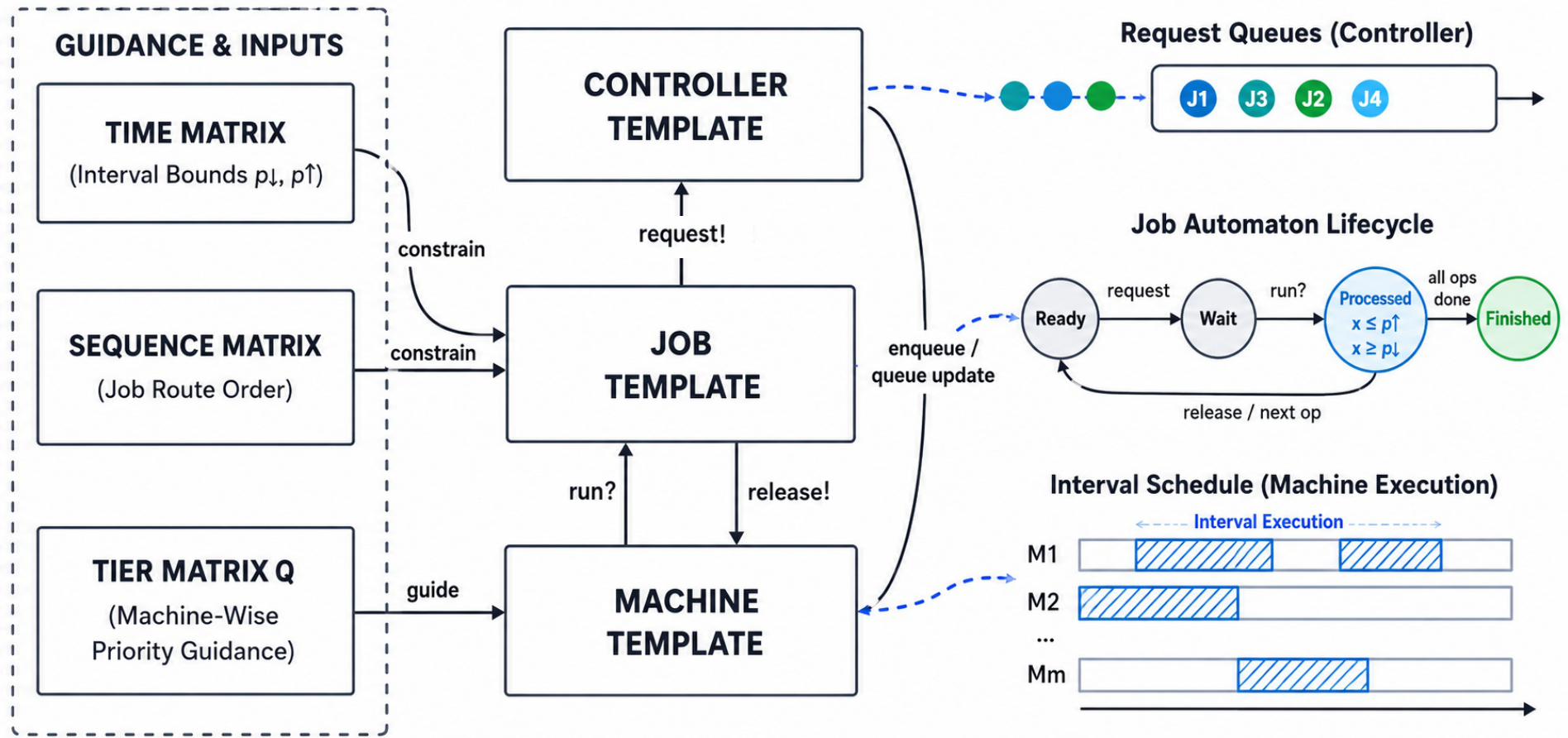
The TAC model represents residual machine-sequence uncertainty and continuous processing-time uncertainty through three reusable timed-automata templates: Job, Machine, and Controller. For a generic
n-job,
m-machine instance, the network contains one Job automaton per job, one Machine automaton per machine, and one Controller. The Job template is parameterised by
, the Machine template by
, and the Controller carries no formal parameter. Shared data provide interval bounds and job routes; the Controller maintains request queues, and the Machine template consults
when selecting among currently waiting requests.
Figure 4 summarises the interaction among the three templates, while
Section 5.2,
Section 5.3 and
Section 5.4 detail their transition semantics.
To implement the timed-automata representation in the proposed framework, we use the UPPAAL Statistical Model Checking (UPPAAL-SMC) tool as the modelling, simulation, and statistical-verification environment [
40,
41]. Each job, machine, and residual sequencing decision is represented through timed-automata templates whose clocks, guards, invariants, and synchronisation channels describe temporal evolution and resource interactions. The partial-order information learned by RAPO-RL is transferred to TAC primarily through the tier matrix
, which guides queue-level machine selection rather than imposing every learned relation as a global hard execution prerequisite; same-tier conflicts remain available for online completion. This implementation supports statistical model checking of sampled timed executions and analysis of completion-time distributions under interval processing-time uncertainty.
5.2. Job Automaton
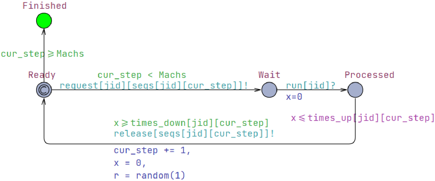
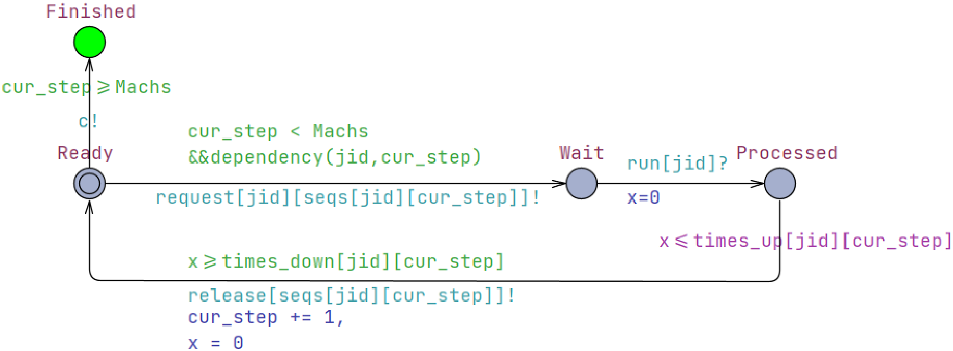
Each job is represented by a parameterised automaton with the principal locations Ready, Wait, Processed, and Finished. From Ready, a job requests the machine required by its next operation and enters Wait. Once admitted by the corresponding Machine automaton, it synchronises into Processed and resets its local operation clock to zero.
Let x be that local clock and let the current operation have duration interval . The Processed location uses the invariant , and its completion transition uses the guard . Thus, the operation may complete at any time satisfying . After completion, the job releases the machine, advances its operation index, and returns to Ready; after all operations have been processed, it enters Finished.
The state transitions and timing constraints of the Job automaton are illustrated in
Figure 5.
5.3. Controller Automaton
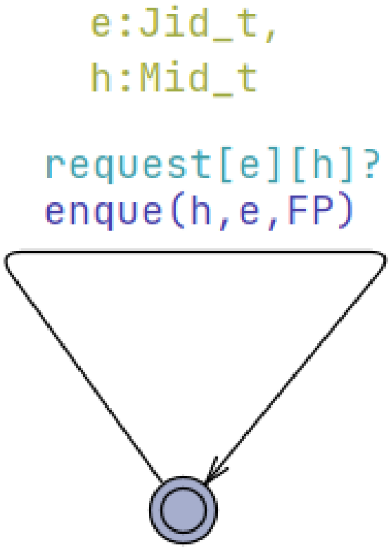
The Controller receives the machine requests emitted by the Job automata and inserts them into the corresponding waiting queues. Its self-loop uses together with the synchronisation to receive any currently enabled job-machine request. This mechanism represents the possible interleavings when several jobs issue requests concurrently.
Figure 6 shows the Controller template and its request-handling transition structure.
5.4. Machine Automaton
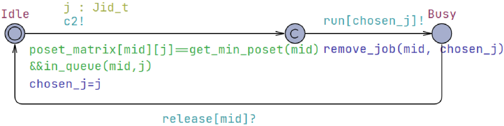
Each machine is represented by an automaton whose operational locations are Idle, a committed selection location
C, and Busy. When machine
is idle and its queue is non-empty, let
denote the set of jobs currently waiting for that machine. The automaton identifies the minimum priority tier
and forms the candidate set
UPPAAL selects a candidate through with the guard . The committed location prevents time from elapsing during machine assignment and therefore avoids artificial waiting.
The corresponding machine-selection and processing transitions are shown in
Figure 7.
5.5. Guided Nondeterministic Completion
The tier matrix guides rather than hard-constrains the UPPAAL selection mechanism.
If , the lower-tier operation is preferred when both requests are currently waiting. The comparison is evaluated only over the current queue: a higher-tier operation is therefore not blocked solely because a lower-tier operation has not yet entered the queue. This queue-level priority semantics allows the timed-automata model to adapt the realised machine sequence to the evolving temporal state.
If , the two operations belong to the same tier and their relative order remains unresolved. When several same-tier jobs are simultaneously available, , the select construct generates alternative legal execution branches. These branches complete the machine-sequencing alternatives intentionally retained by RAPO-RL.
The resulting execution semantics preserves flexibility in two ways. Same-tier jobs retain an explicit nondeterministic choice, while queue availability can also make a currently available higher-tier job execute before a lower-tier job that has not yet entered the queue. Thus, guides the realised machine sequence without imposing machine idling or a global hard execution order.
5.6. Statistical Model Checking
For the job-shop models considered here, exhaustive state-space exploration may become computationally prohibitive as residual branching grows. The final timed-automata model is therefore assessed with UPPAAL-SMC, which samples stochastic timed behaviour without exhaustively enumerating the complete state space.
Let
t denote the global observation clock used for the completion-time analysis. For a specified time bound
T, the principal time-bounded completion query is
UPPAAL-SMC estimates the probability that all jobs complete within the specified bound and also returns sampled completion-time behaviour that can be summarised by probability-density outputs, sample means, and confidence information.
The resulting statistics reflect both the discrete choices retained in the machine partial order and the continuous variation of processing times within their intervals. These results are model-based estimates under the UPPAAL-SMC stochastic semantics, with uncertainty quantified by the reported confidence information; they do not represent a uniform aggregation over all nondeterministic execution paths.
5.7. Monte Carlo Robustness Evaluation
Monte Carlo sampling is used at two distinct stages. During RAPO-RL training, a small sample set provides the terminal robustness reward defined in
Section 4.5.4. After the learned tier matrix
is transferred to TAC, UPPAAL-SMC independently evaluates the completed timed model and reports completion-time and time-bounded statistics. The interval-makespan midpoint remains the nominal criterion used for comparison with established IJSP methods.
6. Experiments and Results
The experiments evaluate seven aspects of RAPO-RL-TAC: nominal schedule quality under the conventional midpoint criterion, statistical significance across matched benchmark instances, robustness to PPO/GNN training randomness, computational and structural efficiency, the contributions of partial-order learning and queue-level completion, sensitivity to the determinacy threshold and open-edge budget, and the additional temporal information provided by UPPAAL-SMC. These aspects are examined through benchmark comparison with paired significance testing, random-seed robustness analysis, computational profiling and residual-conflict analysis, controlled ablation, hyperparameter sensitivity analysis, and statistical model checking.
6.1. Experimental Setup and Evaluation Procedure
RAPO-RL is evaluated as an instance-specific optimiser, with a dedicated policy trained independently for each benchmark instance. Accordingly, the experiments assess per-instance optimisation rather than cross-instance generalisation. For each instance, training uses 10,000 PPO update iterations, parallel environments, , the determinacy threshold , and Monte Carlo samples for terminal robustness evaluation. Every 100 updates, deterministic checkpoint evaluation is performed for the current instance and the best checkpoint is retained; inference then uses greedy edge selection. Processing-time interval bounds remain fixed throughout optimisation and evaluation. The open-edge budget is fixed a priori to for every reported RAPO-RL-TAC run and is not tuned per benchmark instance. All experiments were conducted under Windows 11 with 16 GB of random-access memory (RAM), using Python 3.10.5, PyTorch 2.11.0, CUDA 12.6, and UPPAAL 5.0.0.
After greedy inference,
and
are fixed and the TAC stage is run independently 30 times for each instance. Each exported
.uctr trace is decoded from Machine selection events into a complete per-machine permutation
. Holding this permutation fixed, the makespan is evaluated once at the lower processing-time bounds and once at the upper bounds, yielding
Table 2 reports
over the 30 completed traces; UPPAAL-SMC statistics are analysed separately in
Section 6.7.
6.2. Comparative Evaluation on IJSP Benchmarks
6.2.1. Benchmark Performance Comparison
The principal comparison uses 14 benchmark instances: ORB1–ORB5 and LA16–LA24. Nominal schedule quality is measured by the midpoint of the interval makespan. Let the reported midpoint value of method
a on instance
i be
and let
denote the benchmark lower bound. The relative gap for each method–instance pair is defined as
The mean gap is the arithmetic average of these relative gaps over the 14 instances, with lower values indicating better nominal schedule quality. Descriptive benchmark results are reported here using per-instance midpoint values and mean relative gaps; paired inferential testing across the same 14 instances is reported separately in
Section 6.2.2.
The PNS and GA values are taken from the comparison study of Díaz et al. [
7], with the original PNS method described by Lei [
6]. The fEABC and Fast Elitist Artificial Bee Colony with Local Search (fEABC-LS) results were obtained from our reimplementation of the method in [
8] on the same 14 instances. Because this reproduced benchmark set is broader than that reported in the original fEABC study, the corresponding columns should be interpreted as reproduction results rather than transcribed literature values.
RAPO-RL-TAC achieves a mean midpoint makespan of 998.59, improving on PNS and GA by 2.92% and 1.63%, respectively. The reproduced fEABC and fEABC-LS variants achieve lower mean midpoint makespans, by 0.77% and 2.12%, respectively. At the instance level, RAPO-RL-TAC attains the lowest midpoint on LA21 and LA24 while retaining machine-order flexibility for subsequent timed-automata completion. Its mean relative gap to the listed lower bounds is 6.65%.
6.2.2. Statistical Significance Analysis
To assess whether the per-instance differences in
Table 2 are systematic across the benchmark set, paired two-sided Wilcoxon signed-rank tests were conducted between RAPO-RL-TAC and each comparison method. The 14 matched benchmark instances constitute the paired observations, with one midpoint value from RAPO-RL-TAC and one corresponding midpoint value from the comparison method for each instance. The 30 TAC traces used to obtain the RAPO-RL-TAC midpoint for an instance are therefore not treated as independent samples in this test. The Wilcoxon procedure provides a non-parametric paired comparison without requiring normally distributed instance-level differences.
Table 3 reports the Wilcoxon statistic
W, the two-sided
p-value, and the win/tie/loss (W/T/L) count from the perspective of RAPO-RL-TAC, where a win denotes a lower midpoint makespan. Statistical significance is assessed at
.
The comparison with PNS is statistically significant (
,
), with RAPO-RL-TAC obtaining a lower midpoint on 13 of the 14 instances. The difference relative to GA is also significant (
,
), with 12 wins and 2 losses. In contrast, the difference between RAPO-RL-TAC and the reproduced fEABC results is not statistically significant (
,
). For fEABC-LS, a significant difference is observed (
,
), but the direction favours fEABC-LS, which obtains a lower midpoint on 11 of the 14 instances. These results refine the descriptive comparison in
Table 2: statistical evidence supports the lower midpoint performance of RAPO-RL-TAC relative to PNS and GA, while no significant difference is established relative to fEABC and fEABC-LS remains stronger under the conventional midpoint criterion. Nevertheless, RAPO-RL-TAC achieves lower midpoint makespans than fEABC on 6 of the 14 instances and than fEABC-LS on 3 instances, including the lowest values among all compared methods on LA21 and LA24.
6.3. Random-Seed Robustness Analysis
Training randomness is evaluated separately from the stochasticity of timed-automata execution. For each of the 14 benchmark instances, three independent PPO/GNN training runs were conducted using random seeds 10, 20, and 30. Each run starts from an independently initialised learning process and produces its own learned representations
and
. For each training seed, the learned representation is then fixed and evaluated through 30 independent TAC executions using the same procedure defined in
Section 6.1. The mean midpoint makespan over these 30 TAC traces is used as the seed-level observation. The three seed-level mean midpoint makespans constitute the independent observations used to summarise training-seed variability for each instance.
Across the three seed-level observations, we report the arithmetic mean, sample standard deviation (Std), and two-sided 95% confidence interval computed using Student’s
t distribution with two degrees of freedom.
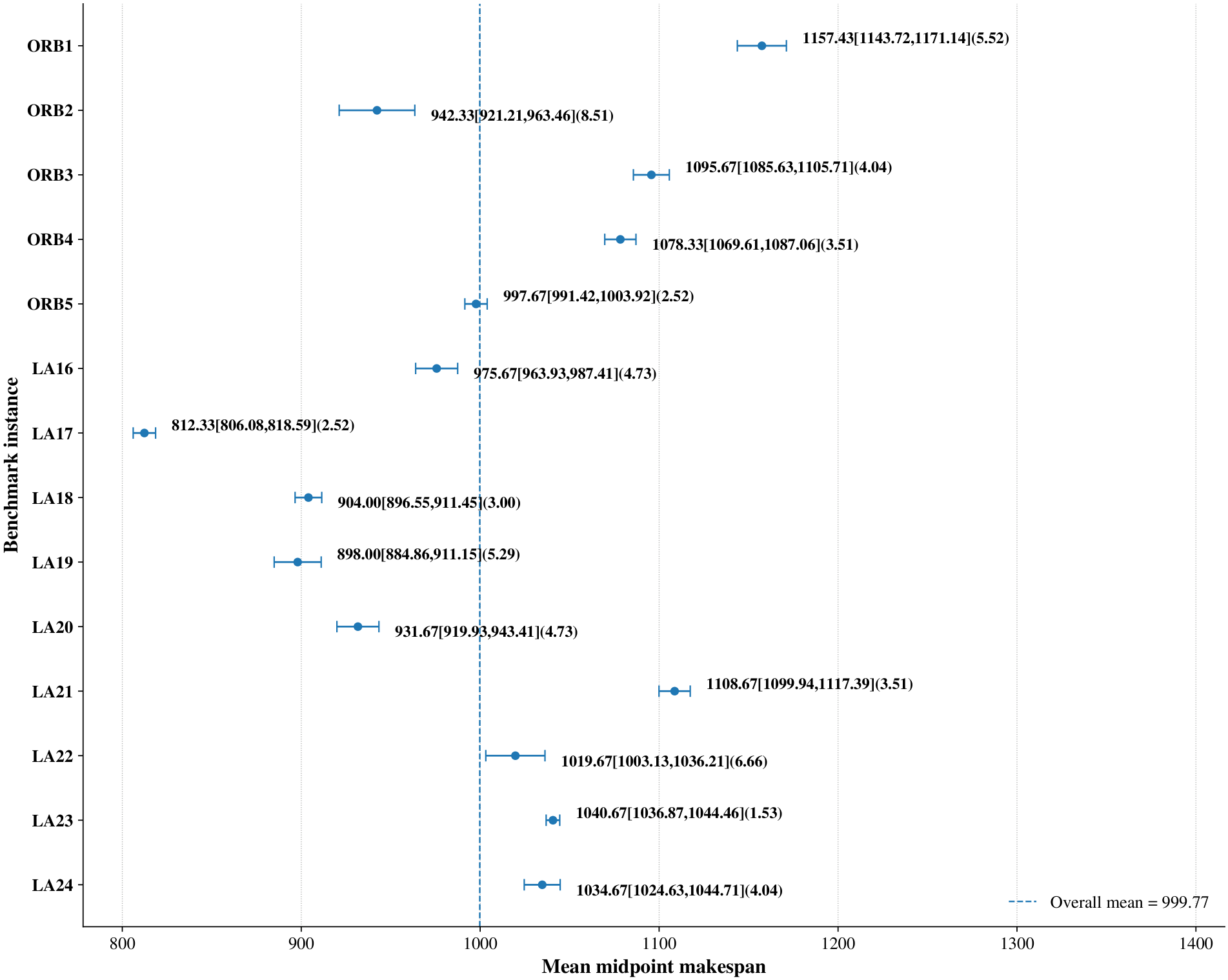
Figure 8 is a horizontal interval plot that summarises these statistics for all 14 benchmark instances. Each row corresponds to one instance: the circular marker denotes the mean midpoint makespan across the three training seeds, the horizontal error bar spans the corresponding 95% confidence interval, and the adjacent annotation reports “Mean[95% CI Lower, 95% CI Upper](Std)”. The vertical dashed line marks the overall mean of the 14 seed-averaged midpoint values, providing a common reference across instances.
The seed-level variability is small relative to the magnitude of the midpoint makespans. Across the 14 instances, the sample standard deviation ranges from 1.53 to 8.51. The coefficient of variation remains below 1% for every instance, with an average of approximately 0.43% and a maximum of approximately 0.90%. The average of the 14 seed-averaged midpoint values is 999.77, which is close to the mean midpoint of 998.59 reported in
Table 2; the absolute difference is 1.18, or approximately 0.12%. Under the three tested training seeds, the resulting schedule quality is therefore relatively stable and remains consistent with the performance level observed in the primary benchmark experiment.
6.4. Computational and Structural Efficiency Analysis
To quantify computational cost and the structural reduction produced by the learned partial order, we record training, inference, TAC, and residual-conflict metrics for the same 14 ORB and LA benchmark instances. In the main experimental campaign, multiple instance-specific training jobs are executed concurrently, so their elapsed times are affected by shared computational resources and do not provide a directly comparable per-instance reference. We therefore profile each benchmark instance separately under the same within-instance parallel-environment configuration, recording the wall-clock time required for each environment to complete 1000 training episodes. The resulting values are reported as reference measurements of single-instance training cost. Inference time is averaged over repeated greedy-inference measurements, and TAC time is the mean wall-clock time per run over the 30 independent TAC executions for each fixed learned representation.
For structural comparison, let
denote the number of initial same-machine conflict relations and
the number left unresolved after RAPO-RL inference. For a
instance,
, whereas for a
instance,
. We report the machine-conflict reduction ratio as
The resulting computational and structural efficiency metrics are reported in
Table 4. The training-time column represents single-instance profiling measurements under the same
configuration, while inference time and TAC time are obtained from repeated measurements and 30 independent executions, respectively. The table also reports the initial machine-conflict relations, unresolved edges after RAPO-RL inference, and the corresponding reduction ratio.
The single-instance profiling results show a clear increase for the larger instances, whereas post-training inference remains below 6 s for all tested instances. Mean TAC execution time remains within 12–18 s per run. During training, the maximum observed peak CPU/GPU memory across instances of the same scale is 1.51/1.79 GB for the group and 2.15/8.30 GB for the group. These measurements indicate that the dominant computational cost is associated with offline learning, while inference and timed-automata completion incur substantially smaller wall-clock costs under the evaluated environment.
As shown in
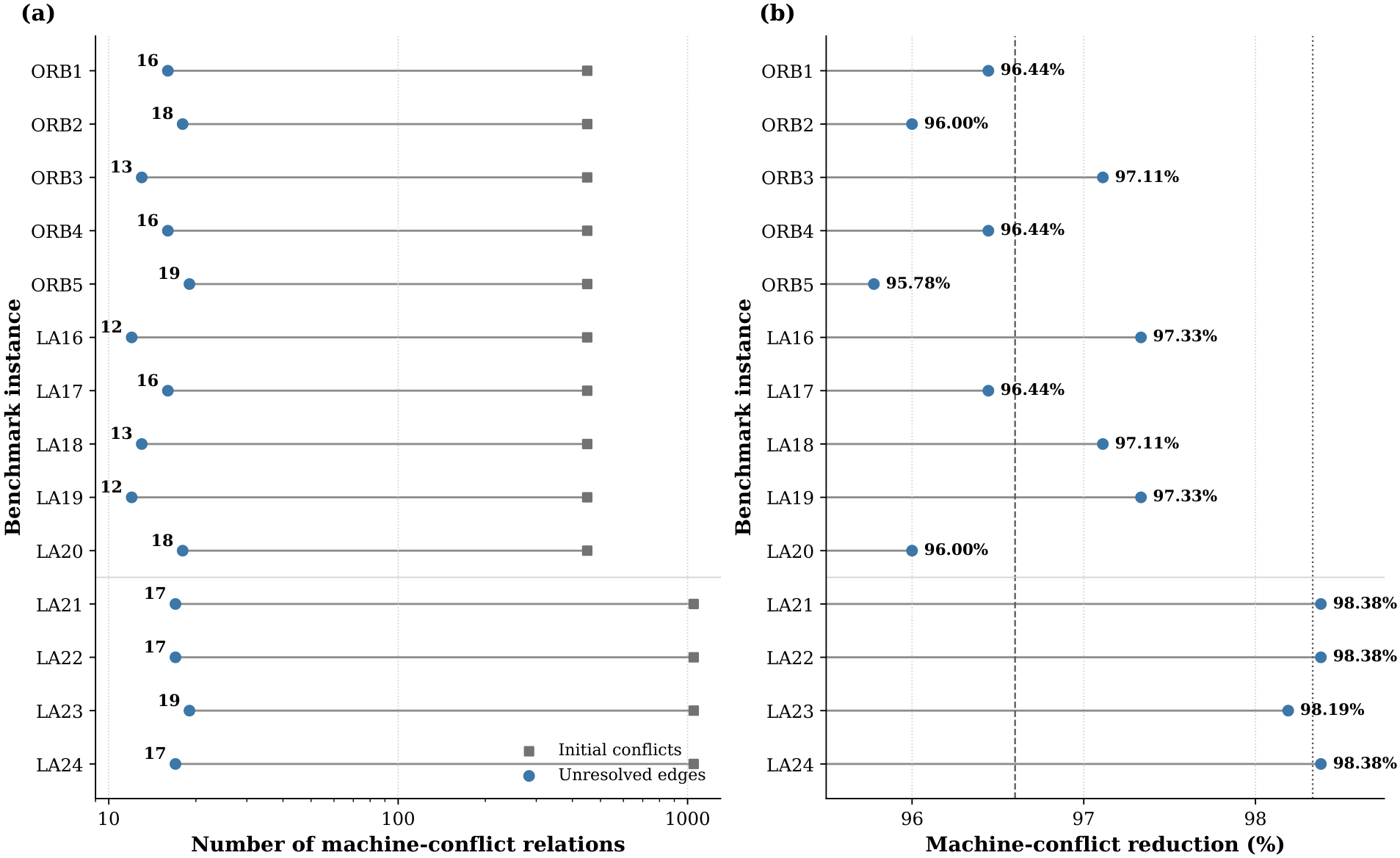
Figure 9, RAPO-RL leaves only 12–19 unresolved machine-conflict relations for TAC. The reduction ratio ranges from 95.78% to 97.33% for the
instances, with a mean of 96.60%, and from 98.19% to 98.38% for the
instances, with a mean of 98.33%. These percentages quantify reduction in machine-conflict relations rather than an exhaustive UPPAAL state-space reduction. Because UPPAAL-SMC evaluates stochastic timed behaviour through statistical sampling rather than exhaustive symbolic enumeration, exact exhaustive state or branch counts are not directly reported; the initial/residual conflict counts, runtime, and memory measurements are therefore used as computational and structural indicators of the residual decision space.
6.5. Ablation Study
Four configurations are compared. Reinforcement-learning-only (RL-only) resolves all machine conflicts through the learned policy and omits timed-automata completion; statistical-model-checking-only (SMC-only) removes the learning stage; Hard-constraint enforces learned dependencies before queue admission; and RAPO-RL-TAC uses the learned tiers only to prioritise currently waiting requests. The RAPO-RL-based variants use the same open-edge budget
, so the Hard-constraint comparison isolates how the learned relation is interpreted by the timed-automata model.
Figure 10 shows the additional
dependency(jid,cur_step) guard used by the Hard-constraint Job template; the dependency must be satisfied before queue admission.
The ablation study selects four instances ABZ9, FT20, LA21, and LA24 to assess the contributions of partial-order learning and timed-automata completion under structurally different job-shop settings. These four instances are drawn from three classical benchmark families, namely ABZ, FT, and LA [
49,
50,
51], and span different job–machine configurations and instance scales, thus forming a representative and heterogeneous subset for mechanism-level evaluation of the proposed framework. ABZ9 originates from the Adams–Balas–Zawack benchmark family and represents a larger-scale benchmark configuration compared with several conventional small-sized instances. FT20 originates from the Fisher–Thompson benchmark family and provides a different job–machine configuration from the other selected instances. LA21 and LA24 are selected from the Lawrence benchmark family and use the
configuration considered in the main evaluation, providing additional cases from the larger Lawrence instance group. This combination allows the ablation study to examine the contribution of each RAPO-RL-TAC component across distinct scheduling structures, providing a more informative mechanism-level comparison of partial-order learning, timed completion, and hard enforcement.
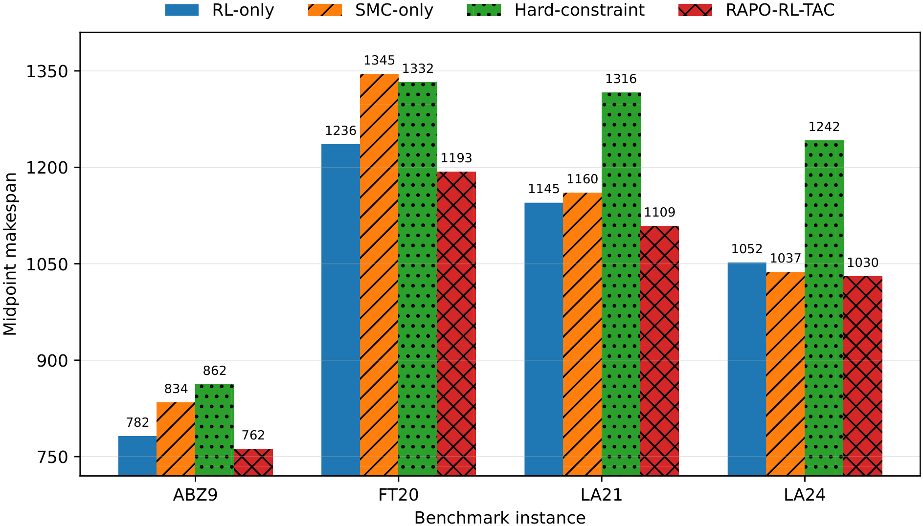
As shown in
Figure 11, RAPO-RL-TAC achieves the lowest midpoint makespan on all four ablation instances, with a mean of 1023.50 compared with 1053.75 for RL-only, 1094.00 for SMC-only, and 1188.00 for Hard-constraint. This corresponds to reductions of 2.87%, 6.44%, and 13.85%, respectively. The largest deterioration occurs under hard enforcement, supporting the use of learned relations as queue-level guidance rather than pre-queue prerequisites. Because the ablation covers four representative instances, these results should be interpreted as mechanism-level evidence rather than a general dominance result.
6.6. Hyperparameter Sensitivity Analysis
A brief sensitivity study is conducted for the temporal-determinacy threshold and the machine-wise open-edge budget , which are fixed to and in the main experiments. The four ablation instances ABZ9, FT20, LA21, and LA24 are used so that the sensitivity analysis remains aligned with the mechanism-level evaluation. For each parameter setting, the same training seed is used and all remaining training settings are held fixed; the resulting learned representation is evaluated using the same 30-run TAC protocol as the main experiments. One parameter is varied at a time, with and .
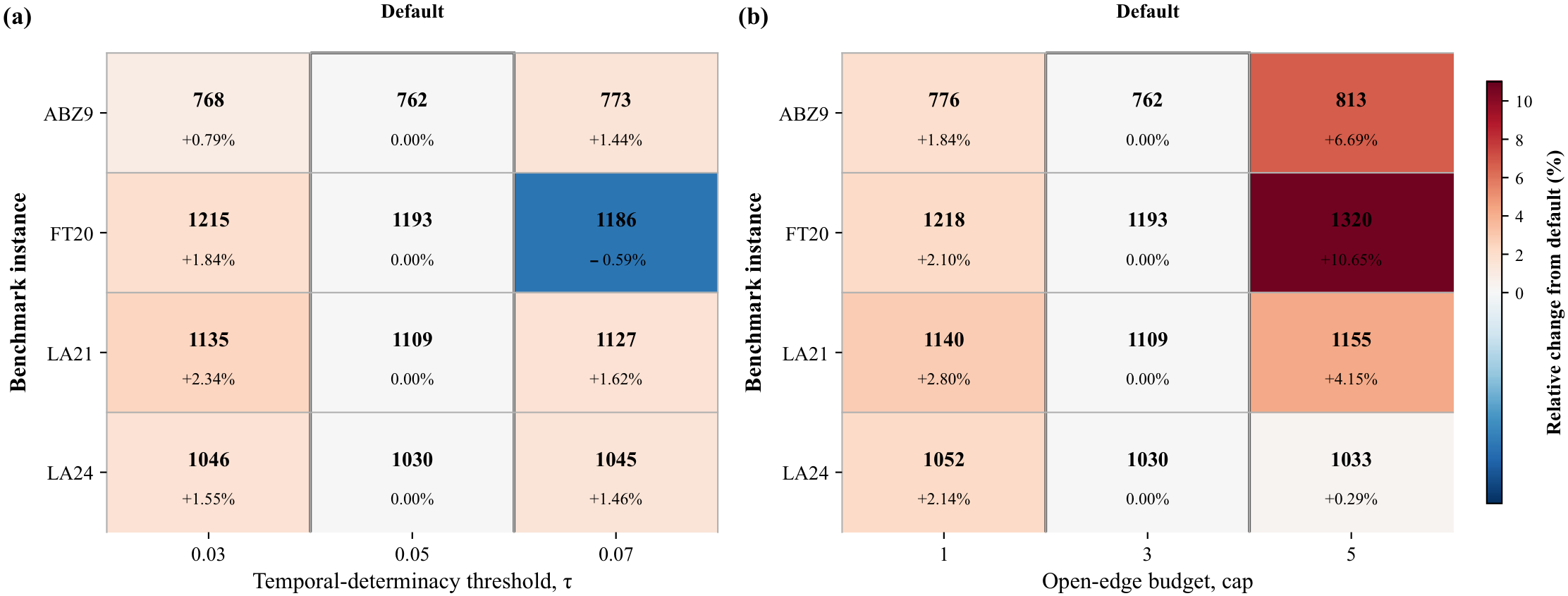
The sensitivity results for
and
are summarised in
Figure 12. The figure presents the tested parameter settings and the corresponding midpoint makespan variations relative to the default configuration.
For the threshold study, the four-instance mean midpoint makespans are 1041.00, 1023.50, and 1032.75 for , 0.05, and 0.07, respectively. Thus, gives the lowest average among the tested values. At the instance level, ABZ9, LA21, and LA24 also attain their lowest midpoint at , whereas FT20 is slightly lower at (1186) than at the default setting (1193).
The open-edge budget exhibits a clearer pattern over the evaluated settings. The four-instance mean midpoint makespans are 1046.50, 1023.50, and 1080.25 for , 3, and 5, respectively; relative to , these correspond to average increases of approximately 2.25% and 5.54% for and . The default budget produces the lowest midpoint on all four tested instances. This pattern is consistent with the intended trade-off: a smaller budget can reduce retained temporal flexibility, whereas a larger budget leaves more residual machine-order ambiguity for timed completion.
6.7. Statistical Model Checking Assessment
The SMC experiment complements the midpoint benchmark by characterising timed executions after
is transferred to TAC. UPPAAL-SMC reports completion-time distributions, sample statistics, confidence information, and time-bounded completion probabilities, thereby providing temporal information that is not represented by the scalar midpoint criterion. Time-bounded completion probability is conceptually aligned with makespan service-level measures used in uncertain job-shop research [
46].
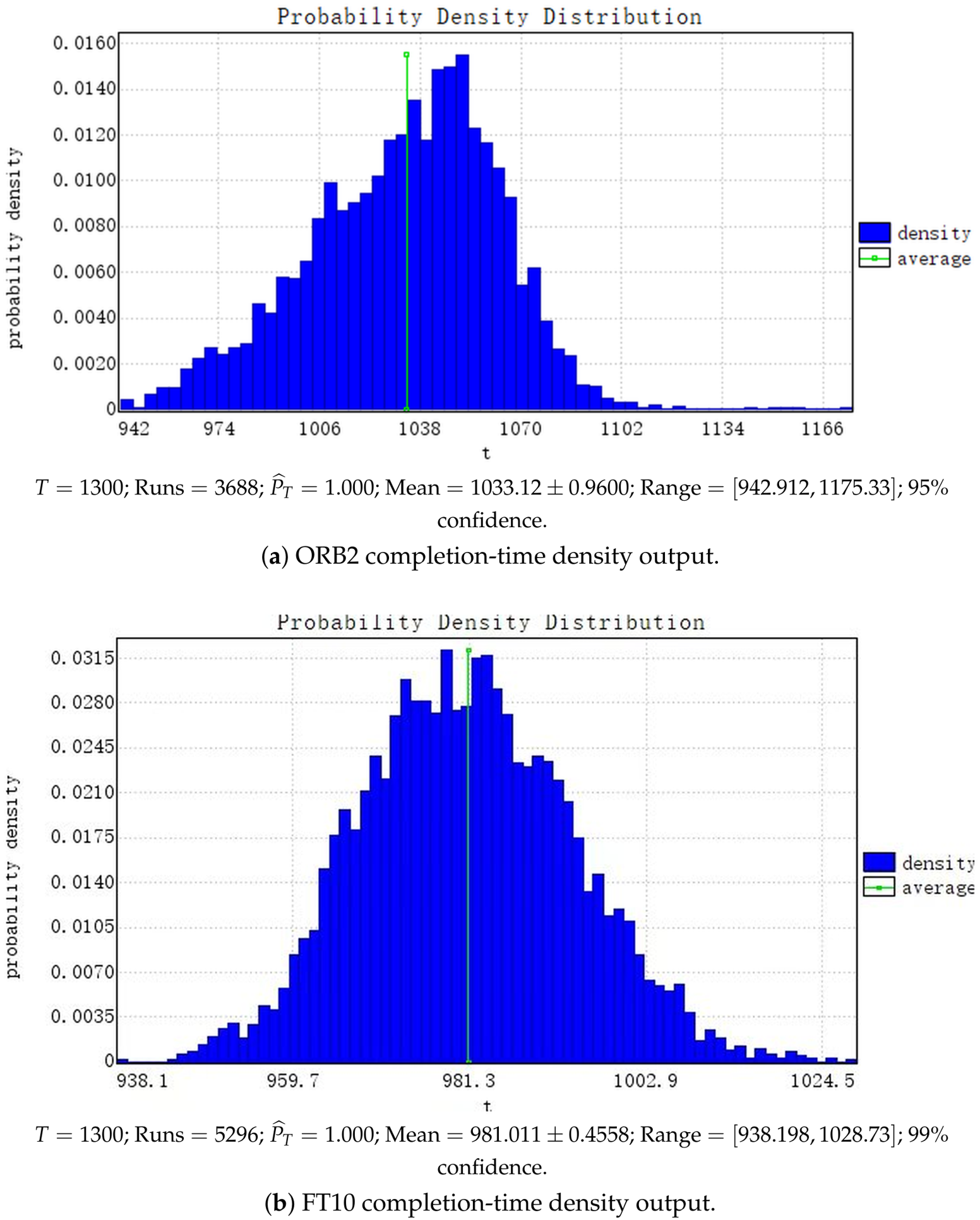
Two representative cases, ORB2 and FT10, are evaluated using a common time bound of .
As shown in
Figure 13, all sampled executions in both cases finish within
, yielding
. ORB2 exhibits a markedly wider observed completion-time range than FT10, indicating greater temporal variability under the sampled UPPAAL-SMC execution semantics.
6.8. Discussion
The benchmark and statistical comparisons show that RAPO-RL-TAC maintains competitive nominal schedule quality across the evaluated IJSP instances while retaining timing-sensitive machine-order relations for subsequent completion. Its mean midpoint makespan is 998.59, compared with 1028.67 for PNS and 1015.17 for GA, corresponding to mean improvements of 2.92% and 1.63%, respectively. The paired Wilcoxon tests further show that these differences are statistically significant: RAPO-RL-TAC obtains lower midpoint makespans than PNS on 13 of the 14 matched instances (, ) and than GA on 12 instances (, ). The reproduced fEABC obtains a lower mean midpoint of 990.91, but the difference from RAPO-RL-TAC is only 0.77% and is not statistically significant (, ). The reproduced fEABC-LS achieves the lower overall mean midpoint of 977.87 and is statistically favoured in the paired comparison (, ), with a lower midpoint on 11 of the 14 instances. At the same time, RAPO-RL-TAC obtains lower midpoint makespans than fEABC on 6 instances and than fEABC-LS on 3 instances, and achieves the lowest midpoint among all compared methods on LA21 and LA24. Taken together, these results show that RAPO-RL-TAC remains competitive under the conventional midpoint objective while preserving the partial-order flexibility required by its timed-completion mechanism.
The random-seed analysis indicates that the observed schedule quality is relatively stable across the three independently trained PPO/GNN seeds. Across the 14 benchmark instances, the sample standard deviations range from 1.53 to 8.51, while the coefficient of variation remains below 1% for every instance, with an average of approximately 0.43% and a maximum of approximately 0.90%. Moreover, the overall mean of the seed-averaged midpoint values is 999.77, only approximately 0.12% different from the mean value of 998.59 in the primary benchmark experiment. These results indicate limited performance variation under the three tested training seeds.
The computational and structural measurements further clarify where the workload of the framework is concentrated and how much scheduling ambiguity is retained for TAC. In the single-instance reference profiles, training time ranges from 3826 to 4471 s for the instances and from 24,127 to 25,109 s for the instances. Post-training inference remains below 6 s for all evaluated instances, and mean TAC execution time ranges from 12 to 18 s per run. The observed peak CPU/GPU memory increases from 1.51/1.79 GB for the group to 2.15/8.30 GB for the group, indicating that the measured computational burden is concentrated primarily in offline training. Structurally, only 12–19 same-machine conflict relations remain unresolved after RAPO-RL inference. The mean machine-conflict reduction reaches 96.60% for the instances and 98.33% for the instances. These results show that RAPO-RL resolves the large majority of same-machine conflicts before timed execution while retaining a small subset for state-dependent completion. The reported percentages quantify reduction in machine-conflict relations and do not represent exhaustive UPPAAL state-space reduction.
The ablation study provides direct mechanism-level evidence for the complementary roles of partial-order learning and timed completion. Across ABZ9, FT20, LA21, and LA24, RAPO-RL-TAC achieves a mean midpoint makespan of 1023.50, compared with 1053.75 for RL-only, 1094.00 for SMC-only, and 1188.00 for Hard-constraint, corresponding to reductions of 2.87%, 6.44%, and 13.85%, respectively. RAPO-RL-TAC also obtains the lowest midpoint on each of the four evaluated instances. The deterioration observed when either the learned partial-order stage or the timed-completion stage is removed supports the complementary contribution of the two stages. The substantially larger deterioration under Hard-constraint further supports using the learned precedence information as queue-level guidance, allowing TAC to retain state-dependent flexibility during execution. The sensitivity results are consistent with this interpretation. For , 0.05, and 0.07, the four-instance mean midpoint makespans are 1041.00, 1023.50, and 1032.75, respectively, so the default provides the lowest average among the tested thresholds, although FT20 is slightly better at . For , 3, and 5, the corresponding means are 1046.50, 1023.50, and 1080.25, and yields the lowest midpoint on all four tested instances. Within the evaluated ranges, these patterns indicate that the adopted settings provide a reasonable balance between resolving sufficiently determinate conflicts before execution and retaining a controlled amount of temporal flexibility for TAC.
The UPPAAL-SMC analysis provides a complementary view of schedule behaviour under interval-valued processing times. For both ORB2 and FT10, all sampled executions complete within the common bound , giving . However, their observed completion-time distributions differ substantially: ORB2 spans approximately 942.91–1175.33, whereas FT10 spans approximately 938.20–1028.73. The markedly wider range for ORB2 indicates greater temporal variability under the sampled execution semantics. These results illustrate that statistical model checking can reveal distributional and time-bounded execution characteristics that are not represented by the scalar fixed-sequence midpoint used in the benchmark comparison.
Several limitations of the present study should be acknowledged. First, RAPO-RL is currently trained separately for each benchmark instance, and cross-instance generalisation has therefore not been evaluated. Second, information currently flows only from RAPO-RL to TAC, and the outcomes of formal temporal analysis are not used to update the learned policy. Third, owing to time and computational-resource constraints, the random-seed analysis is based on three independent PPO/GNN training seeds, and the hyperparameter sensitivity study considers three values for each parameter on four ablation instances. These evaluations provide evidence on training-seed variability and local parameter behaviour within the tested settings, while broader validation across additional training runs and parameter configurations remains necessary.
7. Conclusions
This study established RAPO-RL-TAC, a reinforcement-learning-guided formal framework for the Interval Job Shop Problem (IJSP), demonstrating that selectively partitioning machine-order decisions between RAPO-RL and TAC effectively balances schedule quality and temporal flexibility under interval uncertainty. By resolving most machine conflicts prior to execution, this approach substantially reduces the residual decision space while retaining critical uncertainty-sensitive relations. Comparative experiments confirm that this selective strategy preserves essential scheduling flexibility when optimal sequences depend on actual temporal realizations, while maintaining competitive nominal schedule quality. Furthermore, the ablation results show that integrating RAPO-RL and TAC effectively reduces the makespan of IJSP solutions. Statistical model checking complements the optimisation results by revealing completion-time variability across sampled timed executions, providing a broader view of schedule behaviour under interval uncertainty. In conclusion, RAPO-RL-TAC provides a robust methodology for mitigating decision complexity, preserving sequence flexibility, and rigorously assessing temporal performance in the IJSP.
Future work will focus on extending the framework to larger and more diverse IJSP instances, evaluating cross-instance generalisation, conducting broader random-seed and parameter studies, and developing bidirectional interaction between RAPO-RL and TAC so that outcomes from formal temporal analysis can enhance learning-based scheduling decisions.