Collaborative Optimization of Ladle Furnace Operating Parameters Using Prediction Models and Case-Guided Genetic–Tabu Search

Abstract

Intelligent control of the ladle furnace (LF) process and its endpoint is essential for product quality and stable continuous casting. Existing studies mainly address endpoint prediction or operating-parameter recommendation. Prediction models rarely provide multivariable operating schemes directly, whereas recommendation models often suffer from insufficient coordination among modules and complex commissioning. This study proposes a collaborative LF operating-parameter optimization method combining endpoint prediction with case-guided genetic–tabu search. Given the initial heat state and target endpoint temperature, the method treats electric energy input, power-on duration, and key material additions as decision variables, evaluates each candidate using temperature and composition prediction models, and coordinates the variables through a unified objective. A dynamic weighting mechanism coupling generational annealing with feasible-population temperature-error feedback balances endpoint quality against resource input. Case-based reasoning guides population initialization, while a real-coded genetic algorithm and tabu search strengthen global exploration and local exploitation. For 400 independent historical heats, the method obtained a recommendation satisfying all model constraints for every heat. Relative to the corresponding historical operations, the mean recommended quantities of lime, slag agent, aluminum granules, high-carbon ferromanganese, electric energy input, and power-on duration were reduced by 6.98%, 12.79%, 9.34%, 8.85%, 7.89%, and 8.95%, respectively. Case-guided initialization improved first-generation solution quality and early convergence, whereas tabu search enhanced mid-to-late local refinement. The method converts existing endpoint-prediction capability into coordinated multivariable operating recommendations.

1. Introduction

The ladle furnace (LF) is a key secondary-metallurgy unit linking the basic oxygen furnace or electric arc furnace to continuous casting. It performs molten-steel heating, desulfurization, deoxidation, fine composition adjustment, and inclusion control; consequently, its endpoint temperature and composition directly affect casting stability and product quality. An excessively high endpoint temperature increases electricity consumption, refractory erosion, and the difficulty of controlling temperature loss, whereas an insufficient temperature may require reheating, delay production, or even interrupt casting. An unsuitable charging practice also wastes alloys and slag-forming materials and can increase the electrical energy demand through material thermal effects. Previous studies of intelligent LF control, thermodynamic analysis, and ladle heat transfer have demonstrated the close relationship between endpoint control and energy utilization [1,2,3,4,5]. Therefore, determining electric energy input, processing time, and material additions while ensuring endpoint quality is essential to stable LF operation, energy conservation, and carbon-emission reduction.

Research on intelligent LF refining has mainly followed two routes: endpoint prediction and operating-parameter recommendation. Endpoint prediction estimates the final process state from the initial heat conditions and process records, thereby supporting quality assessment and subsequent adjustment. For example, Guo et al. developed an online endpoint-temperature control model based on big-data learning [6], and Beden et al. combined random forests with semantic reasoning for predictive analysis of steelmaking [7]. Other studies have addressed multi-output prediction, joint tap-temperature and power-consumption control, endpoint-temperature presetting, and ensemble regression [8,9,10,11,12,13,14,15,16]. To improve adaptation to operating regimes, case retrieval, dynamic regression ensembles, and information-interaction enhancement have been introduced [17,18,19]. Nonlinear representation and robustness have further been improved through expert-knowledge/deep-network fusion, dynamic outlier ensembles, heterogeneous ensembles, IF-ZCA-DNN, and mechanism–GA–BP models [20,21,22,23,24]. CBR-based error correction, explainable modeling, PSO–LSTM, mechanism–data residual compensation, and thermodynamic–statistical hybrid models have also broadened the available methods [25,26,27,28,29]. Overall, current models can predict endpoint temperature and composition with high accuracy; however, operators must still compare the predictions with process targets and determine electric energy, power-on duration, and material adjustments from experience, so coordinated multivariable operating schemes are not generated directly.

Unlike endpoint prediction, operating-parameter recommendation directly determines alloy additions, slag-forming materials, and power-supply schedules [30]. Existing studies cover alloy-addition prediction and element-yield modeling [31,32], as well as energy and schedule optimization. Kothari et al. developed a real-time ferroalloy-addition optimizer based on target composition and economic objectives [33]; Regulski et al. embedded power-on-duration prediction in coordinated control of the ladle metallurgy station and continuous casting [34]; and Song et al. proposed a power-saving process for a 120 t LF [5]. These studies extend operating recommendations from alloy calculation to power supply, auxiliary materials, and processing time. Nevertheless, the models are generally developed for individual control objects and therefore employ different inputs, thresholds, correction factors, and mechanistic assumptions. When connected sequentially, mismatched interfaces and inconsistent local decisions can prevent endpoint quality, energy input, and material input from being evaluated coherently within the same candidate scheme. Mechanistic and prediction models have also been embedded in operation optimization. Jawahery et al. established a thermophysical model for online optimization and control of the electric arc furnace [35], while Tian et al. embedded an AdaBoost.IR soft sensor in robust LF operation optimization to coordinate endpoint-temperature stability with electric energy, refining time, and slag quantity [36]. Nevertheless, a unified coupling of multiple endpoint-prediction interfaces with multivariable operation optimization remains underdeveloped, and the relative priority assigned to end-point quality and resource input is not adjusted as candidate schemes evolve. Moreover, combined predictors, material-batch rules, and the historical support domain render the problem nonconvex, nondifferentiable, and multimodal [37]. To address these issues, this study proposes a collaborative LF operating-parameter optimization method based on prediction models and case-guided genetic–tabu search. The proposed method encapsulates the temperature and composition predictors as a unified candidate-evaluation interface. The normalized temperature-deviation and resource-input index terms form the aggregate objective, while electric energy input and material additions are treated as decision variables. Candidate schemes are iteratively optimized subject to endpoint-quality, operating-range, and historical-support-domain constraints. Similar qualified heats jointly define the heat-specific reference level, historical support domain, and initial genetic population; dynamic weights adjust the relative importance of the quality and resource objectives; and genetic global search is combined with tabu local search. This design provides a practical method for reusing existing prediction models to generate coordinated multivariable LF operating recommendations.

2. Prediction–Optimization Control Model

2.1. Problem Description and Objective Function

The proposed prediction–optimization control model comprises two core components: high-accuracy prediction models and a constrained optimization controller. The prediction models characterize the complex relationships between operating parameters and endpoint states. The optimization controller uses these models as candidate evaluators and searches the feasible operating domain for a control scheme that simultaneously satisfies endpoint-quality and resource objectives. Each scheme includes electric energy input, power-on duration, key material additions, and other operating parameters. Its overall workflow is described below.

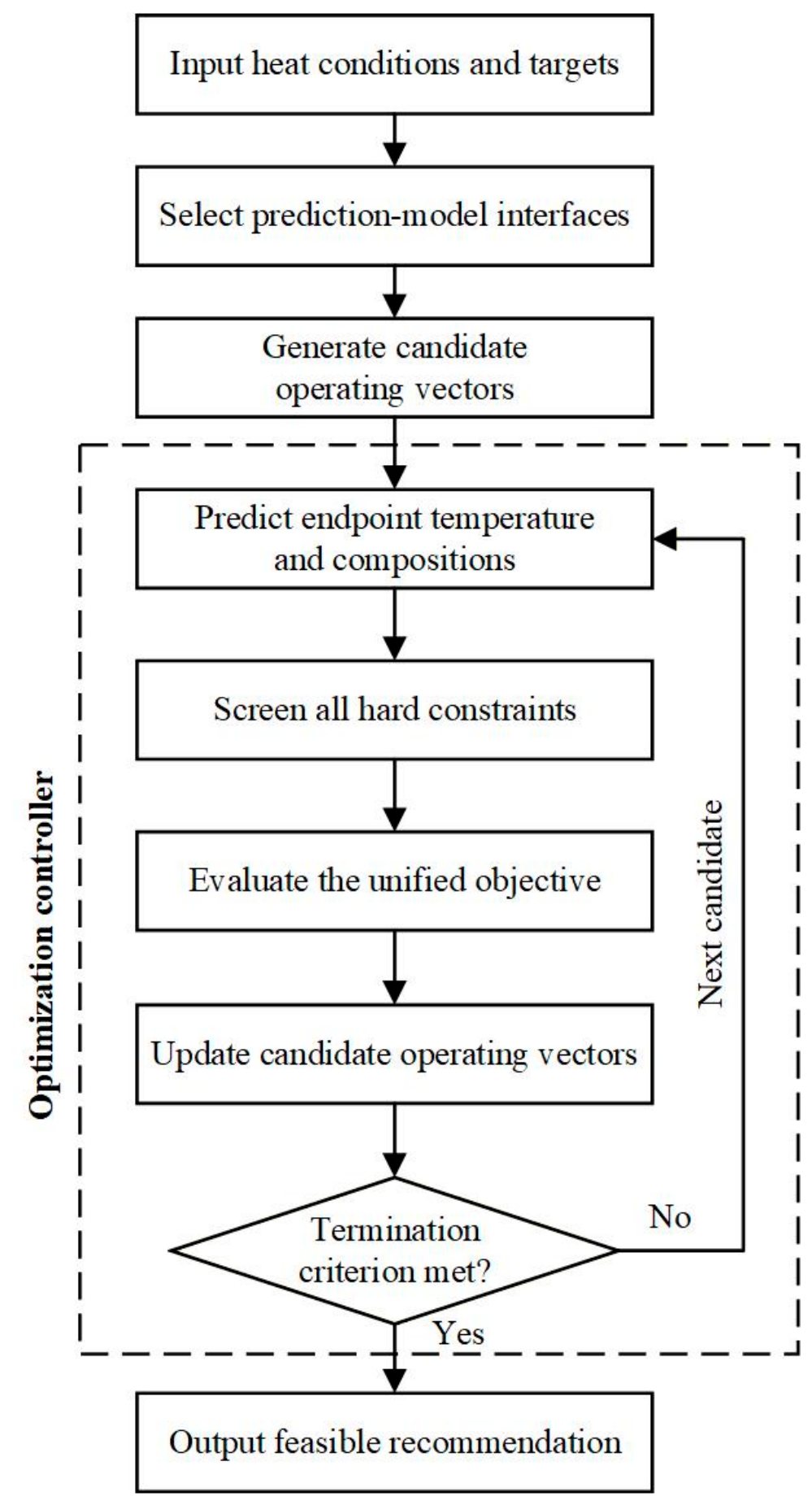
First, the optimization controller generates a set of control parameters within the mechanistic constraints and supplies them, together with the other initial conditions, to the endpoint-prediction models. The models return the process endpoints of greatest interest. For example, the LF endpoint-sulfur model predicts the final sulfur content, and the endpoint-temperature model predicts the final temperature. Second, the controller calculates the aggregate objective value of the candidate parameter set over the multiple optimization objectives. Until the termination criterion is reached, a classical mathematical programming method or a heuristic optimization algorithm adjusts the control-parameter combination and reevaluates the aggregate objective. After termination, the parameter set with the best objective value is selected as the recommended operating reference. The complete workflow is shown in Figure 1.

Within this framework, the objective function consists of two terms, as shown in Equation (1): minimization of the deviation between the predicted and target endpoint temperatures, and minimization of the normalized change in the dimensionless resource-input index constructed from electric energy and key material inputs. Because the two terms have different numerical ranges, the temperature deviation is normalized by the allowable temperature tolerance. The candidate resource-input index is compared with the heat-specific reference resource-input index derived from similar qualified heats and scaled by a characteristic index-change rate with an explicit process interpretation, as expressed in Equation (2).

$$min J_g\left(u\right)={\lambda }_1^{\left(g\right)}{\overline{e}}_T\left(u\right)+{\lambda }_2^{\left(g\right)}{\overline{e}}_C\left(u\right), {\lambda }_1^{(g)}+{\lambda }_2^{(g)}=1$$

(1)

$${\overline{e}}_T\left(u\right)={\displaystyle \frac{\left|g_T\left(x,u\right)-T_{set}\right|}{\Delta T_{tol}}}, {\overline{e}}_C(u)={\displaystyle \frac{C(u)-C_{ref}(x)}{{\delta }_C{C}_{ref}(x)}}$$

(2)

where u is the candidate vector composed of operating variables; x is the heat state known before optimization; $J_g(u)$ is the aggregate objective minimized at generation g; ${\overline{e}}_T\left(u\right)$ and ${\overline{e}}_C(u)$ are the temperature-deviation and resource-input index terms, respectively; and ${\lambda }_1^{(g)}$ and ${\lambda }_2^{(g)}$ are their shared dynamic weights. $g_T(x,u)$ denotes the endpoint-temperature prediction function, $T_{\mathrm{s}\mathrm{e}\mathrm{t}}$ is the externally specified target endpoint temperature, and $\Delta T_{\mathrm{t}\mathrm{o}\mathrm{l}}$ is the allowable temperature tolerance. $C(u)$ and $C_{ref}(x)$ are the resource-input index of the candidate scheme and the reference resource-input index derived from similar cases for the current heat, respectively, and ${\delta }_C$ is the characteristic index-change rate. Although the symbol C is retained in the formulation, it denotes a dimensionless resource-input index rather than a monetary cost. The candidate and case resource-input indices are defined as

$$C(u)={\sum }_{r=1}^R(c_r{m}_r),C_v={\sum }_{r=1}^R(c_r{m}_{v,r})$$

(3)

where R is the number of resource items included in the index and r is the resource-item index; $m_r$ and $m_{v,r}$ are the quantities of resource r in the candidate scheme and historical case v, respectively; $c_r$ is the corresponding median-based normalization coefficient; and $C_v$ is the aggregate resource-input index of historical case v. The coefficients $c_r$ remain constant across all heats and optimization iterations. In this study, R = 6, and the resource items are lime, slag agent, aluminum granules, high-carbon ferromanganese, electric energy input, and power-on duration. To remove differences in units and orders of magnitude, $c_r={\displaystyle \frac{1}{6 \times {\mathrm{m}\mathrm{e}\mathrm{d}\mathrm{i}\mathrm{a}\mathrm{n}}_{\mathrm{nonzero}}(r)}}$. Consequently, when all six inputs equal their respective historical nonzero medians, each contributes 1/6 to C. The resource items and their normalization coefficients are summarized in Table 1.

Table 1. Resource items and normalization coefficients for the dimensionless resource-input index.

Resource Item	Unit	Historical Nonzero Median	Normalization Coefficient
Lime	kg	494.0	3.3738 × 10−4
Slag agent	kg	194.0	8.5911 × 10−4
Aluminum granules	kg	151.0	1.1038 × 10−3
High-carbon ferromanganese	kg	95.0	1.7544 × 10−3
Electric energy input	kWh	4338.66	3.8414 × 10−5
Power-on duration	min	10.30	1.6181 × 10−2

Table 1. Resource items and normalization coefficients for the dimensionless resource-input index.

Resource Item	Unit	Historical Nonzero Median	Normalization Coefficient
Lime	kg	494.0	3.3738 × 10−4
Slag agent	kg	194.0	8.5911 × 10−4
Aluminum granules	kg	151.0	1.1038 × 10−3
High-carbon ferromanganese	kg	95.0	1.7544 × 10−3
Electric energy input	kWh	4338.66	3.8414 × 10−5
Power-on duration	min	10.30	1.6181 × 10−2

If the mean resource-input index of all historical heats were used directly as $C_{ref}(x)$, normal resource differences arising from the initial temperature, steel mass, and ladle thermal state would be confounded with the optimization effect. To establish a reference consistent with the current heat, this study uses the retrieval and reuse stages of case-based reasoning. The case base contains heats of the same steel grade and process route that precede the evaluation set chronologically, have complete production records, and satisfy the endpoint-quality requirements. The state of the current heat and those of the cases are first standardized using case-base statistics, after which the weighted state distance is calculated using Equation (4) [38].

$$d_x(x,x_v)=\sqrt{{\sum }_{q=1}^{Q_x}[{\omega }_q^x{({\tilde{x}}_q-{\tilde{x}}_{v,q})}^2]}$$

(4)

where $d_x(x,x_v)$ is the state distance between the current heat and historical case v; $Q_x$ is the number of state features used for retrieval; q is the feature index; ${\tilde{x}}_q$ and ${\tilde{x}}_{v,q}$ are the corresponding standardized state features; and ${\omega }_q^x$ is the retrieval weight. Retrieval variables include only information available before optimization, such as arrival temperature and composition, steel mass, ladle thermal state, and planned conditions; candidate operations and measured endpoint results are excluded. The $K_c$ nearest cases form the similar-qualified-heat set $N_{K_c}(x)$.

To assign greater influence to cases that more closely match the current state, $C_{ref}(x)$ is calculated using normalized inverse-distance weights:

$${\alpha }_v={\displaystyle \frac{1/[d_x(x,x_v)+{\epsilon }_d]}{{\sum }_{j\in N_{K_c}(x)}1/[d_x(x,x_j)+{\epsilon }_d]}}$$

(5)

$$C_{\mathrm{r}\mathrm{e}\mathrm{f}}\left(x\right)={\sum }_{v\in N_{K_c}\left(x\right)}\left({\alpha }_v{C}_v\right), {\sum }_{v\in N_{K_c}(x)}({\alpha }_v)=1$$

(6)

where ${\alpha }_v$ is the normalized weight of case v, ${\epsilon }_d$ is a small positive constant that prevents division by zero, and j is the case index in the normalization sum. The similar-case set, case weights, and reference resource-input index are calculated once before optimization of each heat and remain fixed throughout all generations.

2.2. Dynamic Weights and Constraints

The weights assigned to the two objective terms should vary during optimization. According to operating practice, when the predicted temperature differs substantially from the target, the model should prioritize accurate temperature control and impose a stronger penalty as the deviation increases. Once the predicted temperature approaches the target, the marginal benefit of further error reduction decreases, and the influence of the temperature penalty should be reduced. This behavior is more consistent with field-control requirements. Accordingly, a dynamic weight is constructed by combining a prior based on generational progress with temperature-error feedback from the feasible population. For ${\lambda }_1^{(g)}$,

$${\lambda }_1^{(g)}={\lambda }_{min}+({\lambda }_{max}-{\lambda }_{min})\{h(g)+[1-h(g)](1-{\tau }_g)q_T(g)\}$$

(7)

$$q_T\left(g\right)={\displaystyle \frac{1}{1+e^{-k\left[{\overline{e}}_T\left(g\right)-b\right]}}}, h\left(g\right)={\displaystyle \frac{e^{-\rho {\tau }_g}-e^{-\rho }}{1-e^{-\rho }}}, {\tau }_g={\displaystyle \frac{g-1}{G_{max}-1}}$$

(8)

$${\overline{e}}_T\left(g\right)=median\{{\overline{e}}_T(u_n)\mid u_n\in P_g^F\}$$

(9)

where $P_g^F$ is the set of candidates satisfying all hard constraints at generation g; ${\overline{e}}_T(g)$ is the median normalized temperature-error term in that generation; $q_T(g)$ is the temperature-error feedback factor; b and k are the feedback transition point and slope, respectively; ${\tau }_g$ is the normalized generation progress; $G_{max}$ is the maximum number of generations; $h(g)$ is a normalized annealing function that decays from 1 to 0; $\rho$ is the annealing decay coefficient; and ${\lambda }_{min}$ and ${\lambda }_{max}$ are the lower and upper bounds of the temperature weight. Equations (7) and (8) give ${\lambda }_1(1)={\lambda }_{max}$ at the first generation and makes the weight approach ${\lambda }_{min}$ in the final generation; during the intermediate stage, temperature-error feedback adjusts the decay rate.

In addition to minimizing the objective function, each candidate scheme must satisfy requirements for endpoint temperature, endpoint composition, operating variables, equipment capability, and similarity to historical operating conditions. Equation (10) bounds the predicted endpoint-temperature error, Equation (11) constrains the predicted values of key compositions, and Equation (12) specifies the basic lower and upper bounds of the operating variables.

$$|g_T(x,u)-T_{set}|\le \Delta T_{tol}$$

(10)

$$y_{i,min}\le g_i\left(x,u\right)\le y_{i,max}, i\in \{S,Mn,Als,O,\cdots \}$$

(11)

$$l_j\le u_j\le h_j,j=1,2,\dots ,D$$

(12)

where $g_i(x,u)$ is the prediction function for endpoint component $i$; $y_{i,min}$ and $y_{i,max}$ are its permitted lower and upper bounds, respectively; and $i\in \{S,Mn,Als,O\}$ denotes the key constraints explicitly optimized in this study, namely sulfur (S), manganese (Mn), acid-soluble aluminum (Als), and dissolved oxygen (O). Other elements that are insensitive to the current decision variables or can be calculated reliably from charging rules are constrained by the steel-grade process specification. $D$ is the number of decision variables, $u_j$ is the $j$th operating variable, and $l_j$ and $h_j$ are its lower and upper bounds. These bounds jointly reflect the historical data range, equipment capability, and steel-grade operating practice.

Although the preceding quality and operating bounds enforce explicit process limits, equipment and operating capability must also be considered to prevent the optimizer from exploiting extreme parameter combinations to obtain an apparently favorable objective value. The similar-case set retrieved by Equation (4) is therefore reused to calculate the minimum weighted distance from a candidate operating vector to local historical cases. The 95th percentile of the corresponding distance distribution in the historical data is used as the support-domain threshold, as defined in Equations (13) and (14).

$$d_H(z)=min\{d(z,z_v)\mid v\in N_{K_c}(x)\}\le {\tau }_{0.95}$$

(13)

$$d(z,z_v)=\sqrt{{\sum }_{q=1}^Q[{\omega }_q{(z_q-z_{v,q})}^2]}$$

(14)

where z is the standardized state–operation vector formed from the current heat state and candidate operation; $z_v$ is the standardized state–operation vector of historical case $v$; $v$ is the case index; $d(z,z_v)$ is the weighted Euclidean distance between candidate vector z and case $v$; $Q$ is the number of features in $z$; $q$ is the feature index; $z_q$ and $z_{v,q}$ are the corresponding standardized components at feature $q$; and ${\omega }_q$ is the associated feature weight. $d_H(z)$ is the minimum distance between the candidate scheme and the historical cases in $N_{K_c}(x)$, and ${\tau }_{0.95}$ is the 95th-percentile threshold of analogous historical distances. Here, $d_x$ retrieves cases using only the pre-optimization state, whereas $d_H$ additionally includes the candidate operation to determine whether a specific scheme lies within the local support of the historical data. The two distances therefore serve different purposes while sharing the same case set. A candidate is deemed infeasible when $d_H$ exceeds ${\tau }_{0.95}$.

2.3. Integration of the Prediction Models

The objective and constraints above define how candidate schemes are evaluated, while their endpoint temperature and composition are calculated by the corresponding prediction models. The temperature, S, Mn, Als, and O models integrated here use historical variables from the same LF line under consistent definitions, but model-specific datasets were constructed from records with valid labels for each endpoint.

Endpoint temperature is predicted using our previously published mechanism–data hybrid method [28]. The method first uses $k$-means to identify operating regimes and trains a backpropagation neural network with adaptive dropout within each regime. A heat-balance model describes electric energy input, material thermal effects, and heat dissipation, while the data-driven model compensates for mechanistic residuals. The model was trained on 2800 cleaned LF heats collected in 2023 and validated using subsequent production data. After further process optimization, its prediction hit rate within ±5 °C reached 95.73%.

The composition models follow the same operating-regime-specific modeling and residual-compensation strategy as the temperature model. Because the completeness of endpoint labels differs among S, Mn, Als, and O, each model was trained and tested separately using its corresponding valid records collected from January to December 2023. Model inputs are listed in

Table 2. Input variables of the endpoint-prediction models.

Output	Input Variable
Endpoint temperature	Arrival temperature, steel weight, arrival composition, ladle thermal state, waiting time, electric energy input, power-on duration, lime, slag agent, aluminum granules/wire, high-carbon ferromanganese, and deoxidizer
Endpoint S	Arrival S, lime, arrival temperature, slag agent, steel weight, arrival Als, and power-on duration
Endpoint Mn	Arrival Mn, high-carbon ferromanganese, steel weight, arrival temperature, electric energy input, power-on duration, aluminum granules, and slag agent
Endpoint Als	Arrival Als, arrival O and S, aluminum granules/wire, deoxidizer, lime, slag agent, arrival temperature, power-on duration, and steel weight
Endpoint O	Arrival O and Als, aluminum granules/wire, deoxidizer, lime and slag agent, arrival temperature, power-on duration, and steel weight

, and the training-set and independent-test sizes and test performance are reported in

Table 3. Sample sizes and test performance of the endpoint-prediction models.

Output	MAE	RMSE	Hit Rate (%)	Training Set, n	Test Set, n
Endpoint temperature	1.491	3.356	±5/±10 °C: 95.73/99.19	2800	867
Endpoint S	0.00120	0.00170	±0.002/±0.003%: 83.31/91.61	3300	1192
Endpoint Mn	0.00510	0.01980	±0.010/±0.020%: 92.45/99.50	3300	1192
Endpoint Als	0.00499	0.00647	±0.005/±0.010%: 75.25/87.16	3300	1192
Endpoint O	2.3 ppm	3.6 ppm	±5 ppm: 87.20	2000	656

. All endpoint models used the same chronological split: data from January to September 2023 constituted the training set, whereas data from October to December 2023 constituted the independent test set. For each model, the model structure and hyperparameters, missing-value treatment, outlier-screening thresholds, and all preprocessing parameters were determined solely using the training set, whereas the independent test set was used only for final performance evaluation.

A common data-cleaning protocol was applied before chronological partitioning: duplicate heat IDs, records with missing key inputs or outputs, physically impossible negative additions, sensor-failure records, and non-standard production events were removed. Continuous inputs were winsorized using only the 0.5th and 99.5th percentiles of the training data and then standardized using the training-set mean and standard deviation.

MAE and RMSE denote mean absolute error and root mean square error, respectively, and are defined in Equations (15) and (16). In Table 3, temperature errors are reported in °C; S, Mn, and Als errors are expressed as mass fractions in %; and O errors are reported in ppm. The hit rate of Als within ±0.005% is lower than those of the other outputs, partly because this threshold is narrow relative to its process-control interval. In SPHC production, the requirements for Als are relatively lenient. Als is judged against an allowable interval rather than a single point target, and the ±0.010% hit rate is therefore reported as a supplementary indicator. The influence of prediction errors on optimization constraints is further examined in Section 4.2.

$$\mathrm{M}\mathrm{A}\mathrm{E}={\displaystyle \frac{1}{M}}{\sum }_{a=1}^M(|y_a-{\widehat{y}}_a|)$$

(15)

$$\mathrm{R}\mathrm{M}\mathrm{S}\mathrm{E}=\sqrt{{\displaystyle \frac{1}{M}}{\sum }_{a=1}^M[{(y_a-{\widehat{y}}_a)}^2]}$$

(16)

where $M$ is the number of independent-test samples, $a$ is the sample index, and $y_a$ and ${\widehat{y}}_a$ are the measured and predicted values of sample $a$, respectively. Hit rates are calculated using the error thresholds listed in Table 3.

3. Case-Guided Genetic–Tabu Hybrid Algorithm

3.1. Case Initialization and Real-Coded Genetic Search

The combined prediction models, piecewise rules, and hard constraints defined above generally make the objective nondifferentiable and may produce multiple local optima. Direct solution by gradient-based nonlinear programming is therefore unsuitable. To balance exploration across regions with fine local optimization, a genetic algorithm provides the global search framework, while case-based reasoning and tabu local search are embedded as enhancements.

3.1.1. Real-Coded Representation and Genetic Operators

(1)

Population initialization

Because all decision variables are continuous operating quantities, real-valued encoding is used. A chromosome represents a complete candidate control scheme, and each gene corresponds to an adjustable operating parameter expressed directly in its physical units. This representation avoids binary-to-real conversion and introduces no additional discretization error associated with coding length.

The genetic search minimizes $J_g$ in Equation (1). After the feasible population at generation g has been formed, the shared weights for that generation are calculated using Equations (7)–(9), and the parents, offspring, and retained elites are then re-evaluated with the same weights. Considering the characteristics of process optimization, tournament selection, simulated binary crossover (SBX), and the corresponding polynomial mutation operator are adopted [39,40].

(2)

Selection

Tournament selection randomly samples $k$ individuals from the population, where $k$ is the tournament size and is usually 2–5. The best individual among these $k$ candidates enter the mating pool, and the process is repeated until the mating pool is filled. Adjusting $k$ controls the selection pressure: a larger $k$ increases the probability of selecting elite individuals and accelerates convergence. Candidates are ranked directly by the smaller aggregate objective value, without a positive-fitness transformation; the value used in this study is listed in the algorithm-parameter table.

(3)

Crossover

This paper uses SBX to generate continuously varying offspring within the parent’s neighborhood. For parent individuals $p_1$ and $p_2$, two offspring $c_1$ and $c_2$ are generated as follows [39]:

Perform the following operations independently for each gene pair:

Generate a random number $r$ ∈ [0, 1].

Specify the distribution index ${\eta }_c$, a non-negative real number typically between 2 and 5. A smaller value promotes wider exploration, whereas a larger value emphasizes local exploitation; the index controls the proximity of the offspring to their parents.

Calculate the coefficient $\beta$:

$$\beta =(2r{)}^{1/({\eta }_c+1)}, r\le 0.5$$

(17)

$$\beta =[{\displaystyle \frac{1}{2(1-r)}}{]}^{1/({\eta }_c+1)}, r>0.5$$

(18)

Generate the offspring:

$$c_1=0.5[(1+\beta )p_1+(1-\beta )p_2],c_2=0.5[(1-\beta )p_1+(1+\beta )p_2]$$

(19)

SBX therefore produces continuous candidate operations around high-quality parent schemes while retaining a controllable degree of exploratory variation.

(4)

Mutation

Polynomial mutation is also designed for real-coded variables. For parent $p$, the mutated offspring $c$ is generated as follows:

Apply mutation to each gene with a small probability.

Generate a random number $r$ ∈ [0, 1].

Specify the distribution index ${\eta }_m$, which is typically between 20 and 100.

Calculate the perturbation $\delta$. When $r$ ≤ 0.5, $\delta$ is evaluated using Equation (20); when $r$ > 0.5, $\delta$ is evaluated using Equation (21).

$$\delta =[2r+(1-2r)(1-{\delta }_1{)}^{{\eta }_m+1}{]}^{1/({\eta }_m+1)}-1$$

(20)

$$\delta =1-[2(1-r)+(2r-1)(1-{\delta }_2{)}^{{\eta }_m+1}{]}^{1/({\eta }_m+1)}$$

(21)

$${\delta }_1={\displaystyle \frac{p-lb}{ub-lb}},{\delta }_2={\displaystyle \frac{ub-p}{ub-lb}}$$

(22)

where $p$ and $c$ are the gene values before and after mutation; $lb$ and $ub$ are the lower and upper variable bounds; ${\delta }_1$ and ${\delta }_2$ are the normalized distances from $p$ to the lower and upper bounds; ${\eta }_m$ is the mutation distribution index; and $r$ is a uniform random number on [0, 1].

The mutated offspring is calculated using Equation (23):

$$c=p+\delta (ub-lb)$$

(23)

Polynomial mutation adjusts the perturbation scale according to the individual’s position in the search space, keeps the result within the variable bounds, and uses local perturbations to explore candidate schemes that may further reduce the temperature deviation or the resource-input index [40].

3.1.2. Case-Guided Initialization

The similar qualified heats retrieved using Equations (4)–(6) provide not only the reference resource-input index but also historical operating schemes matched to the current heat state. However, if case-based reasoning were used alone as the recommendation model, its output would be limited by case-base coverage and historical operating quality, and abnormal or low-quality cases could affect retrieval. To retain the condition-matching advantage of case knowledge without directly reusing historical schemes, the retrieved cases guide the initial search positions of the genetic algorithm rather than serving as final recommendations.

Specifically, the historical case schemes and their perturbed samples within the bounds form the case-initialized portion of the population, causing the initial population to preferentially cover high-quality feasible regions supported by historical data. The remaining individuals are sampled randomly within the variable bounds to preserve exploration of new operating combinations. This design reuses the case retrieval, reference resource-input index, and support-domain definitions from Section 2 during optimization and provides a consistent operating-condition basis for the subsequent genetic and tabu searches.

Accordingly, half of the initial population starts near historical feasible schemes, whereas the other half retains the ability to explore operating combinations not previously observed. An individual that violates any hard constraint is discarded and resampled near a similar case or within the variable bounds until a feasible initial population is formed or the specified candidate-generation limit is reached.

3.1.3. Tabu Local Search

Genetic operators can maintain exploration across regions, but the population may still become concentrated in local regions during the middle and late stages. To alleviate search stagnation, every G_L generations, several optimal feasible individuals are selected from the current population as initial solutions for tabu search. For general design of the tabu list, the aspiration criterion, and local reinforcement, see Reference [41]; for tabu search and global optimization approaches in continuous variable spaces, see Reference [42]. Combining the continuity and boundary characteristics of the LF operational variables, this paper employs bounded Gaussian perturbations to generate neighborhood candidates within the normalized decision space.

The specific implementation is as follows: a local search is triggered once every 10 generations, selecting the two best feasible individuals; each local iteration generates 24 neighborhood candidates, with a normalization step ratio of 0.025 and a taboo length of 10, and each elite is allowed to perform up to six local iterations. In each round, the following steps are performed sequentially: neighborhood generation, boundary projection, process discretization, batch endpoint prediction, hard constraint screening, and tabu evaluation. Additionally, the candidate with the minimum objective value is allowed to update the current local solution, and the resulting local optimal feasible solution ultimately replaces the corresponding elite.

3.2. Termination Criteria and Computational Procedure

To avoid comparing aggregate objective values calculated with different dynamic weights, stagnation is evaluated using a fixed-weight comparison index. The main loop terminates when the maximum generation Gmax is reached or when this comparison index fails to improve by more than 10⁻⁴ for Gstop = 24 consecutive generations. The fixed-weight index is used only for termination assessment and does not affect selection under the dynamic objective. The principal computational complexity of the hybrid algorithm can be approximated by Equation (24).

$$O(G_{max}N{C}_s+{\displaystyle \frac{G_{max}}{G_L}}{n}_e{I}_L{n}_N{C}_s)$$

(24)

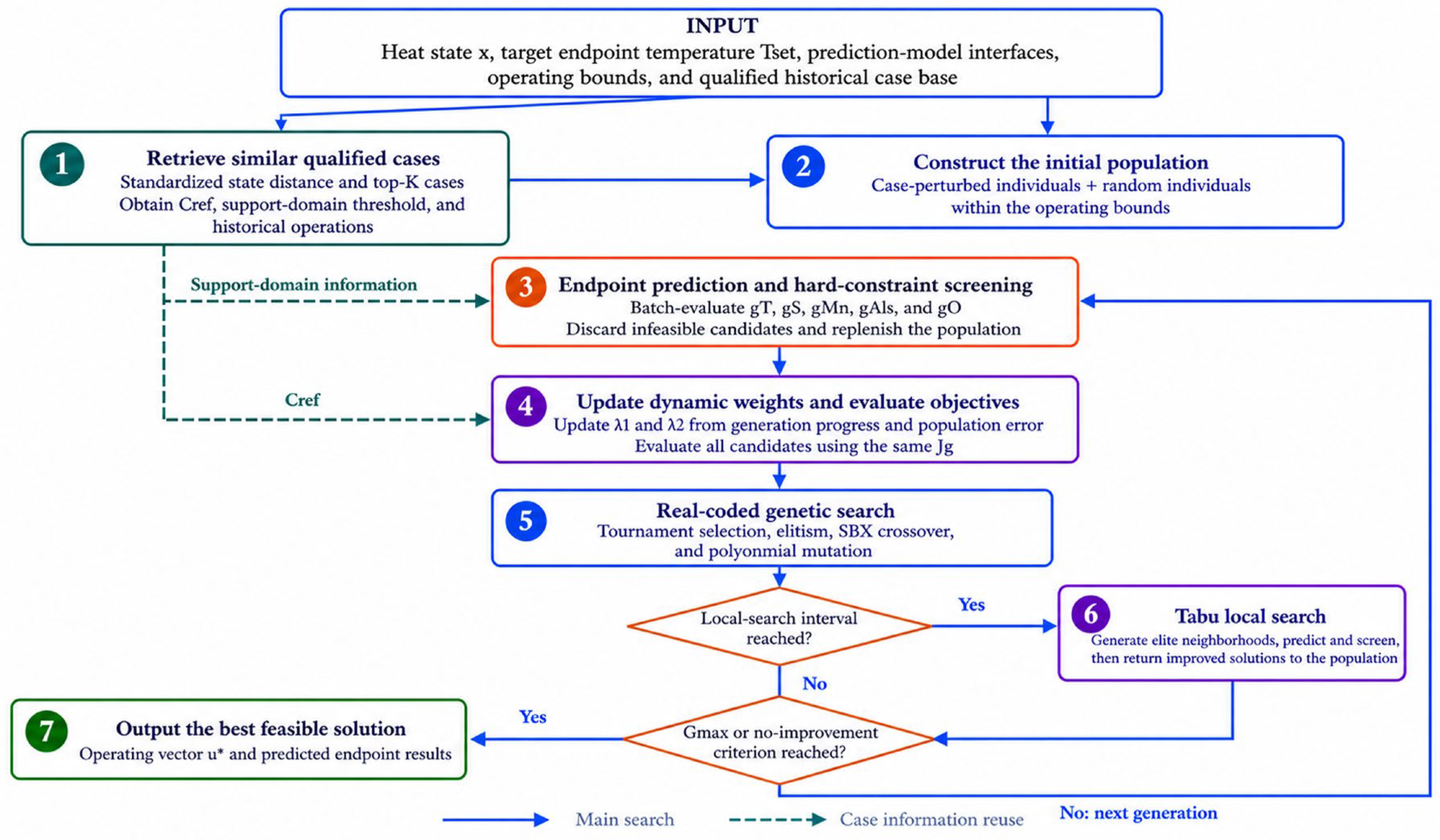
where $G_{max}$ is the maximum number of genetic generations, $N$ is the population size, and $C_s$ is the average cost of invoking all endpoint-prediction models and evaluating the constraints for one candidate. $G_L$ is the local-search interval, $n_e$ is the number of elite individuals entering local search, $I_L$ is the maximum number of local iterations in one tabu search, and $n_N$ is the number of neighborhood candidates generated per local iteration. Candidates within the same generation are predicted in batches, and repeated operations are cached to reduce model-evaluation cost. The complete procedure is shown in Figure 2 and is summarized as follows:

(1)

Input the current heat state $x$, target endpoint temperature $T_{\mathrm{s}\mathrm{e}\mathrm{t}}$, endpoint-prediction-model interfaces, operating bounds, and qualified historical case base. Retrieve similar qualified cases using Equations (4)–(6) to obtain the similar-case set, heat-specific reference resource-input index $C_{\mathrm{r}\mathrm{e}\mathrm{f}}$, historical-support-domain threshold ${\tau }_{0.95}$, and corresponding historical operations.

(2)

Construct the case-initialized individuals from the historical operations of similar cases and their within-bound perturbations, and supplement them with random individuals sampled within the variable bounds to form the initial candidate population.

(3)

Invoke the endpoint temperature and composition prediction models, including $g_T$, $g_S$, $g_{\mathrm{M}\mathrm{n}}$, $g_{\mathrm{A}\mathrm{l}\mathrm{s}}$, and $g_O$, in batches. Check the hard constraints on endpoint quality, operating ranges, and the historical support domain; discard infeasible candidates and replenish the feasible population using the same initialization rules.

(4)

Update the shared dynamic weights ${\lambda }_1$ and ${\lambda }_2$ from the current generation progress and the median temperature error of the feasible population, and calculate $J_g$ for all feasible candidates using the same weight pair.

(5)

Apply tournament selection, elitist retention, SBX crossover, and polynomial mutation to the feasible population to generate the next candidates. When the generation reaches the local-search trigger interval $G_L$, select elite individuals from the current population for tabu search.

(6)

Generate local neighborhoods around the elite individuals, repeat prediction and hard-constraint screening, and select improved solutions according to the tabu list and aspiration criterion. Write the resulting local best feasible solutions back to the genetic population.

(7)

Determine whether the maximum number of generations $G_{\mathrm{m}\mathrm{a}\mathrm{x}}$ has been reached or whether the fixed-weight comparison index has failed to improve by more than 10⁻⁴ for 24 consecutive generations. If neither criterion is met, return to step (3); otherwise, output the best feasible operating vector $u^{\ast }$ and its predicted endpoint results.

Figure 2. Computational procedure of the case-guided genetic–tabu hybrid algorithm.

Figure 2. Computational procedure of the case-guided genetic–tabu hybrid algorithm.

4. Experiments and Discussion

4.1. Dataset and Algorithm Settings

The study considers SPHC steel refined in the LF process of a steel plant, using the same data source as the prediction models. LF operations for this grade comprise molten-steel receipt, crust breaking and slag melting, electric heating, slag formation and deoxidation, composition adjustment, and final soft stirring before departure. According to the production specification, the principal endpoint composition requirements are $[C]\in [0.03, 0.06]$, $[S]\le 0.015$, $[\mathrm{M}\mathrm{n}]\in [0.15, 0.40]$, $[\mathrm{S}\mathrm{i}]\le 0.03$, $[P]\le 0.022$, $[\mathrm{A}\mathrm{l}\mathrm{s}]\in [0.023, 0.040]$, and $[\mathrm{C}\mathrm{a}]\in [15 \mathrm{p}\mathrm{p}\mathrm{m},25 \mathrm{p}\mathrm{p}\mathrm{m}]$. The required molten-steel temperature is 1595 ± 5 °C.

The prediction-model datasets and case base were obtained from January to December 2023. The optimization-evaluation data were collected from production records in January 2024 and were completely disjoint by heat ID from all prediction model training sets, independent test sets, and the case base. The January 2024 production database contained 1147 available heats. After heats with missing arrival-state or endpoint-state information were removed, 943 heats remained. Among the remaining 943 heats, the final evaluation set retained SPHC heats produced on the investigated LF line via the standard process route, for which the six decision variables, prediction-model inputs, target information, and heat identifiers were complete. Recorded values were required to fall within predefined valid ranges jointly determined by expert-based process-plausibility assessment and the 3σ rule. Heats with records of equipment faults, unplanned process termination, or other non-standard events were also excluded. All screening criteria were established before optimization, and inclusion was not determined by optimization performance, recommendation feasibility, or whether the historical endpoint outcome was favorable. This screening yielded 400 heats for optimization evaluation, representing routine SPHC production on the target line under the standard process route.

The case base was screened by steel grade, completeness of key fields, and simultaneous qualification of endpoint temperature, S, Mn, O, and Als. After incomplete records and heats with unqualified endpoints were removed, 911 qualified heats were retained. The time spans and purposes of the data subsets are summarized in

Table 4. Temporal partitioning and purposes of the modeling, case-base, and optimization-evaluation datasets.

Data Subset	Time Span	Number of Heats	Purpose
Prediction-model datasets	Training: January–September 2023; independent testing: October–December 2023	See Table 3 for each model	Model fitting, selection, and independent testing
Case base	January–December 2023	911	Standardization, case retrieval, $C_{\mathrm{r}\mathrm{e}\mathrm{f}}$, support domain, and initialization
Optimization-evaluation data	January 2024	400	Offline recommendation generation and per-heat comparison with historical operation

.

The aggregate resource input is represented by the dimensionless index C. For each resource item, the normalization coefficient is defined as the reciprocal of its nonzero median in the training set divided equally by the number of resource items, so that all resources have equal initial contributions under typical operating conditions.

Table 5. Main parameters of the optimization algorithm.

Parameter	Symbol	Value	Parameter	Symbol	Value
Population size	$N$	20	Maximum generations	$G_{max}$	120
Crossover probability	$p_c$	0.80	Mutation probability	$p_m$	0.09
SBX distribution index	${\eta }_c$	5	Mutation distribution index	${\eta }_m$	20
Case-initialization proportion	${\rho }_c$	0.50	Similar reference cases	$K_c$	35
No-improvement generations	$G_{stop}$	24	Characteristic index-change rate	${\delta }_C$	0.10
Lower temperature-weight bound	${\lambda }_{min}$	0.20	Upper temperature-weight bound	${\lambda }_{max}$	0.85
Sigmoid transition point	$b$	0.55	Sigmoid slope	$k$	10
Tournament size	$k_t$	3	Elite individuals	$n_e$	2
Local-search interval	$G_L$	10	Neighborhood candidates	$n_N$	24
Tabu length	$L_t$	10	Maximum local iterations	$I_L$	6
Weight-annealing decay coefficient	$\rho$	3.0	Neighborhood step-size ratio	$s$	0.025
Effective-improvement threshold	${\epsilon }_{stop}$	10−4	Comparison temperature weight	${\lambda }_{1cmp}$	0.50

lists the main algorithm parameters.

4.2. Results and Analysis

4.2.1. Overall Endpoint-Prediction and Recommended-Operation Results

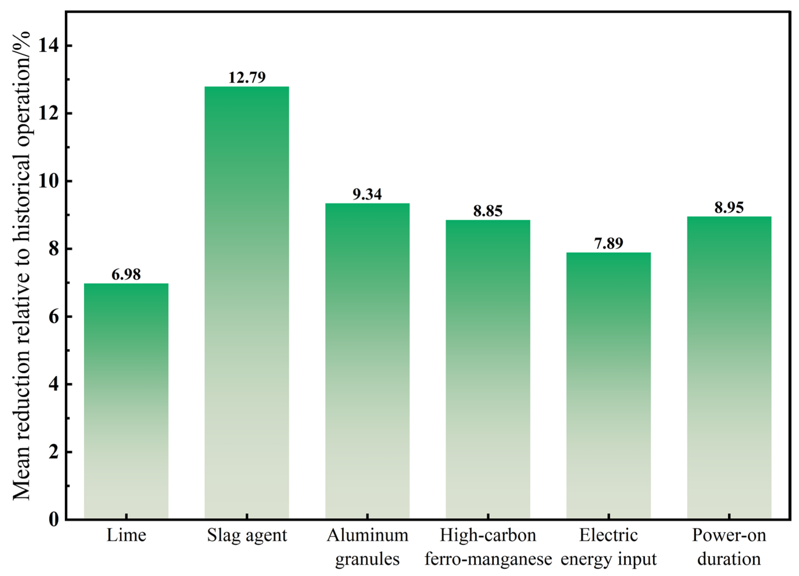
For all 400 heats, the optimizer produced feasible recommendations satisfying the requirements for temperature, S, Mn, Als, O, operating bounds, and the historical support domain. Differences between the recommended and corresponding historical operations were compared for material and energy-input variables to determine whether the optimizer achieved endpoint-quality control by reallocating resource input.

Table 6. Comparison of mean operating quantities between the recommended and historical schemes.

Operating Quantity	Recommended	Historical	Mean Absolute Reduction	Mean Reduction (%)
Lime (kg)	370.66	398.49	27.83	6.98
Slag agent (kg)	125.55	143.97	18.41	12.79
Aluminum granules (kg)	174.62	192.62	17.99	9.34
High-carbon ferromanganese (kg)	70.44	77.28	6.84	8.85
Electric energy input (kWh)	4255.55	4620.15	364.60	7.89
Power-on duration (min)	10.31	11.32	1.01	8.95

lists the mean values of the six principal operating quantities, and Figure 3 shows their relative changes. Electric energy input and power-on duration primarily affect heat input; lime and slag agent jointly alter slag-forming conditions; and aluminum granules and high-carbon ferromanganese provide deoxidation and fine composition adjustment, respectively.

For resource item r in heat i, the absolute reduction is defined as the historical quantity minus the model-recommended quantity. The mean absolute reduction in Table 6 is the average of this quantity over the 400 heats, and the mean reduction is the mean absolute reduction divided by the mean historical quantity.

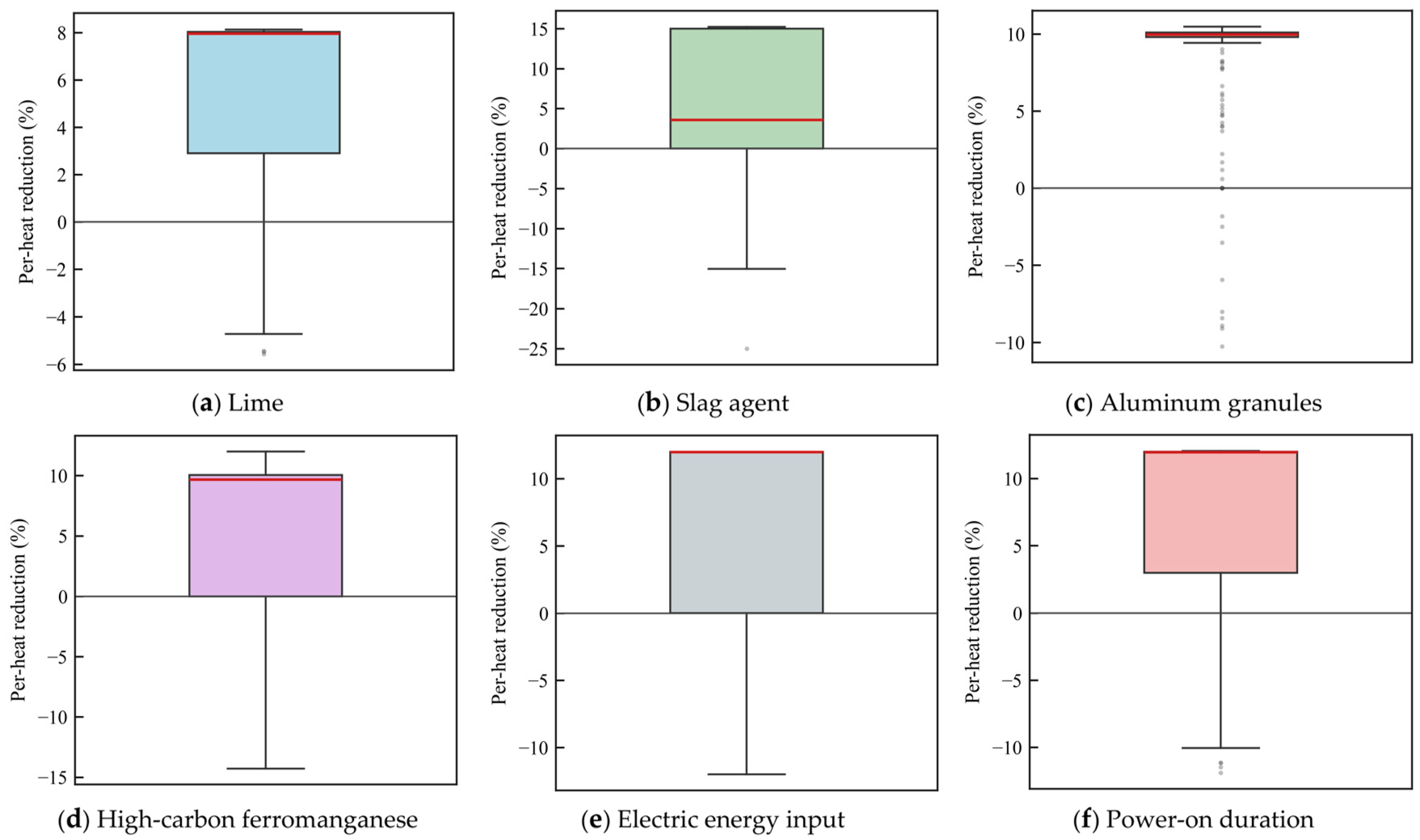
The mean values of all six recommended operating quantities were lower than their corresponding historical values, although the magnitude of reduction differed because of their process functions and allowable adjustment ranges. The mean additions of lime, slag agent, aluminum granules, and high-carbon ferromanganese decreased from 398.49, 143.97, 192.62, and 77.28 kg to 370.66, 125.55, 174.62, and 70.44 kg, corresponding to mean relative reductions of 6.98%, 12.79%, 9.34%, and 8.85%, respectively. Electric energy input and power-on duration decreased from 4620.15 kWh and 11.32 min to 4255.55 kWh and 10.31 min, corresponding to mean relative reductions of 7.89% and 8.95%. Figure 4 and

Table 7. Robust statistics of the per-heat operating-quantity reductions.

Operating Quantity	Median Reduction (%)	Interquartile Range (%)	Heats with No Increase (%)
Lime	7.96	[2.90, 8.04]	97.75
Slag agent	3.57	[0.00, 14.98]	98.00
Aluminum granules	9.96	[9.79, 10.09]	97.00
High-carbon ferromanganese	9.68	[0.00, 10.06]	94.75
Electric energy input	11.99	[0.00, 12.08]	79.00
Power-on duration	11.96	[2.98, 12.00]	91.25

further report the distributions and robust statistics of the per-heat relative reductions.

Figure 4 and Table 7 reveal the between-heat distributions of the recommended operations. Positive values in the boxplots indicate that the recommended quantity is lower than the historical operation, whereas negative values indicate an increase. The boxes for all operating quantities lie predominantly above the zero baseline. In particular, the 25th percentiles of lime, aluminum granules, and power-on duration are clearly positive, indicating positive reductions in at least approximately 75% of the evaluation heats. The lower box edges for the slag agent and high-carbon ferromanganese lie at zero, but their median reductions remain 3.57% and 9.68%, respectively; the median reduction in electric energy input is 11.99%. Thus, the overall adjustment direction remains downward. When the endpoint-temperature, composition, and historical-support-domain constraints are satisfied, the resource objective consequently drives these variables toward their permitted lower levels.

The lower whiskers of some variables extend into the negative region, indicating that the recommended quantities exceed the corresponding historical values for a small number of heats. This result confirms that the method does not impose a uniform proportional reduction on every resource; instead, it allocates resources on a heat-specific basis to balance an overall reduction in resource input against endpoint feasibility. To determine whether the mean reductions were driven by a small number of extreme heats, bootstrap interval estimation, Wilcoxon signed-rank tests, and effect-size analysis were performed on the paired quantity differences for all 400 heats. The results are presented in

Table 8. Statistical tests of the per-heat reductions in the six operating quantities.

Operating Quantity	Mean Reduction	95% BCa Confidence Interval	Holm-Adjusted p-Value	Rank-Biserial Effect Size
Lime (kg)	27.83	[25.89, 29.64]	<0.001	0.993
Slag agent (kg)	18.41	[16.45, 20.55]	<0.001	0.994
Aluminum granules (kg)	17.99	[17.08, 18.86]	<0.001	0.995
High-carbon ferromanganese (kg)	6.84	[6.19, 7.50]	<0.001	0.977
Electric energy input (kWh)	364.60	[327.16, 400.47]	<0.001	0.815
Power-on duration (min)	1.01	[0.93, 1.10]	<0.001	0.940

.

Table 8 shows that the 95% bias-corrected and accelerated (BCa) confidence intervals for the mean reductions in all six quantities lie entirely above zero, and all Holm-adjusted Wilcoxon signed-rank tests yield p < 0.001. The overall reductions are therefore not driven by a few extreme heats. The rank-biserial effect sizes are 0.993, 0.994, 0.995, and 0.977 for lime, slag agent, aluminum granules, and high-carbon ferromanganese, respectively, and 0.940 for power-on duration, indicating a consistent downward direction across most heats. The effect size for electric energy input is 0.815; although lower than those of the other variables, it still indicates a strong directional change. These results agree with Figure 4: individual inputs may increase in a small number of heats to maintain endpoint feasibility, but the overall distributions consistently indicate lower resource input.

To examine the influence of prediction error on hard-constraint screening, the independent-test MAE of each model in Table 3 was used as the error scale for its corresponding output. The allowable prediction intervals for temperature, S, Mn, O, and Als were contracted inward by $\alpha$ times the relevant MAE, with $\alpha$= 0, 0.25, 0.50, and 1.00. The feasible-recommendation acquisition rate is defined as the proportion of evaluation heats for which at least one recommendation satisfying all model constraints is obtained within the prescribed candidate-generation limit. The acquisition rate, temperature error, resource-input index reduction, and runtime under the different contraction levels are compared in

Table 9. Results of the constraint-contraction experiment based on independent-test MAE.

Constraint Setting	Heats with a Recommendation	Feasible-Recommendation Acquisition Rate (%)	MATD (°C)	Resource-Input Index Reduction (%)	P50 Runtime (s)
$\alpha =0$	400/400	100.00	1.789	8.67	0.779
0.25 × MAE	385/400	96.25	1.740	8.45	1.541
0.50 × MAE	373/400	93.25	1.689	8.15	1.439
1.00 × MAE	352/400	88.00	1.500	6.31	1.083

.

In the optimization experiments below, the mean absolute target-temperature deviation (MATD) is defined as the temperature metric, namely, the mean absolute difference between the endpoint temperature predicted for a recommended scheme and the externally specified target temperature. This metric differs from the prediction-model MAE in Table 3, which is calculated relative to measured endpoint temperatures.

As $\alpha$ increases from 0 to 0.25, 0.50, and 1.00, Table 9 shows that the feasible-recommendation acquisition rate decreases to 96.25%, 93.25%, and 88.00%, respectively, while the resource-input index reduction decreases from the baseline value of 8.67% to 8.45%, 8.15%, and 6.31%. Among the heats for which a recommendation is obtained, the MATD decreases progressively from 1.789 °C to 1.500 °C. Contracting the prediction intervals therefore requires candidate temperatures to lie closer to the target and also changes the composition of the feasible heats included in the statistics. The results indicate that moderate constraint contraction can absorb part of the prediction uncertainty while retaining a practical recommendation-acquisition rate.

4.2.2. Dynamic-Weight Evolution and Parameter Sensitivity

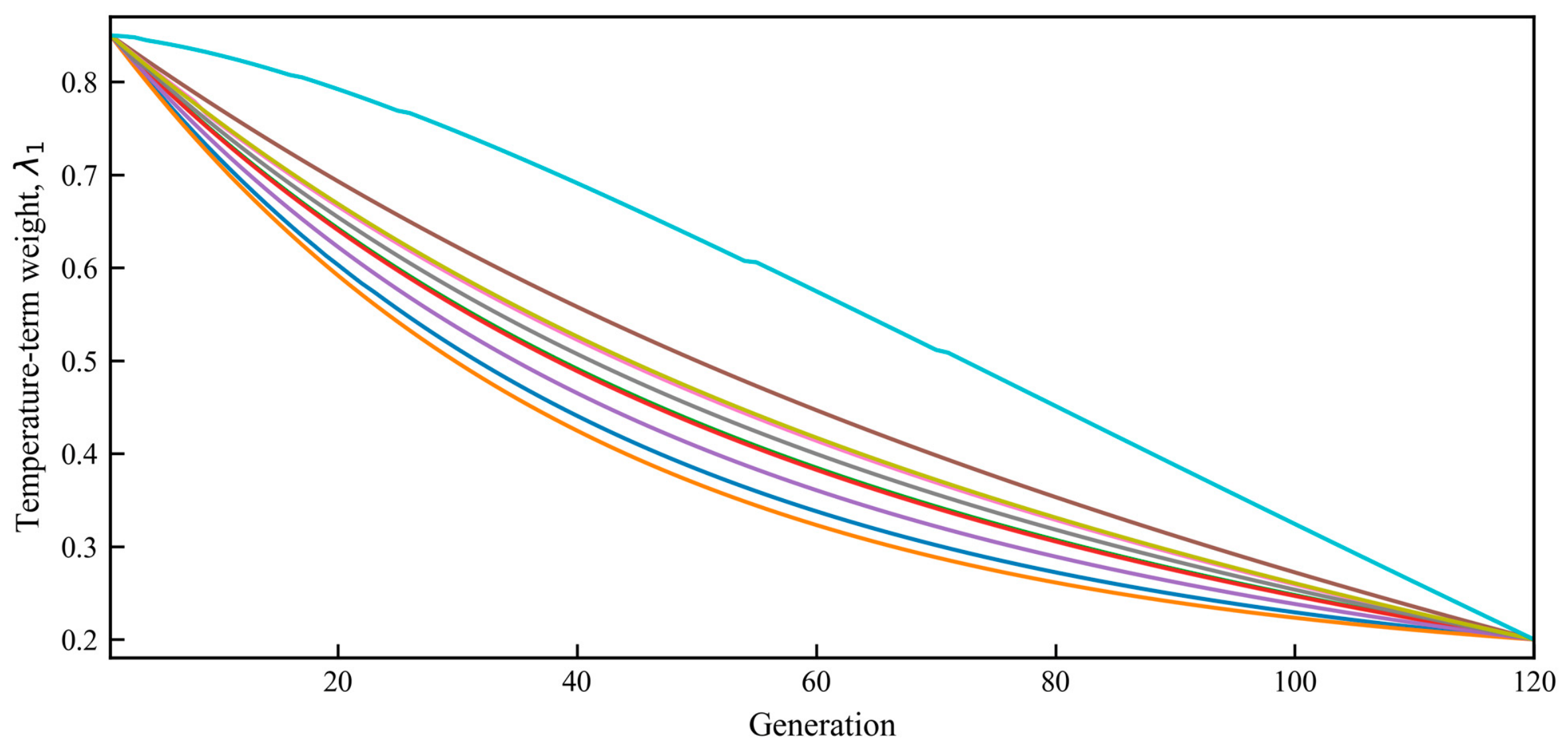
To further verify whether generational progress and feasible-population temperature-error feedback jointly coordinate the two objectives, Figure 5 presents the temperature-term weight trajectories of 10 representative heats over 120 generations. Each trajectory is calculated using Equations (7)–(9). The generational annealing term prescribes a gradual transition from endpoint-feasibility priority to resource optimization, whereas the temperature-error feedback term adjusts the decay rate according to the current feasible population. The resource-input index term weight is determined simultaneously by λ2 = 1 − λ1.

As shown in Figure 5, the temperature weight of every heat starts at its upper bound of 0.85, decreases smoothly as the search proceeds, and approaches the lower bound of 0.20 during the late stage. The trajectories differ visibly in the intermediate stage. Heats with larger feasible-population temperature errors exhibit slower decay to maintain emphasis on endpoint-temperature control, whereas those with smaller errors increase the resource-term weight more rapidly. The weighting mechanism therefore retains a clear process interpretation across the search stages while adaptively adjusting the objective-transition rate according to heat difficulty.

Fixed weights, different sigmoid parameters, and different characteristic index-change rates were further compared on 60 stratified heats; the results are presented in

Table 10. Sensitivity results for the dynamic weights and characteristic index-change rate.

Setting	${\mathit{\delta }}_{\mathit{C}}$	$\mathit{b}$	$\mathit{k}$	MATD (°C)	Feasible-Recommendation Acquisition Rate (%)	Resource-Input Index Reduction (%)
Fixed weights	0.10	–	–	2.167	100.00	9.56
Temperature-oriented	0.10	0.40	8	1.911	100.00	8.87
Baseline setting	0.10	0.55	10	1.960	100.00	9.08
Resource-oriented	0.10	0.80	4	1.989	100.00	9.15
Index-change rate 0.05	0.05	0.55	10	2.023	100.00	9.46
Index-change rate 0.15	0.15	0.55	10	1.869	100.00	8.47

.

Table 10 shows that the MATD values under fixed weights and the baseline dynamic weights are 2.167 °C and 1.960 °C, respectively, while the corresponding resource-input index reductions are 9.56% and 9.08%. Relative to fixed weights, the baseline dynamic weights reduce MATD by 0.207 °C while retaining a resource-input index reduction above 9%. The two alternative sigmoid settings produce MATD values of 1.911 °C and 1.989 °C and resource-input index reductions of 8.87% and 9.15%, indicating limited variation over the tested range. Because the prediction models and constraints are coupled nonlinearly, neither metric varies monotonically with an individual parameter. By contrast, increasing the characteristic index-change rate from 0.05 to 0.15 reduces MATD from 2.023 °C to 1.869 °C while decreasing the resource-input index reduction from 9.46% to 8.47%, revealing a clear temperature–resource trade-off. All six settings achieve a 100% feasible-recommendation acquisition rate, indicating that the baseline parameters lie within a stable feasible region.

Further, to test whether the conclusions obtained with equal typical contributions from the six resources depend on a single coefficient setting, 20 evenly spaced sampled heats and 10 random seeds were used. Taking the baseline coefficients as the reference, one of the six resource coefficients was increased or decreased by 20% at a time, producing 12 one-factor perturbation schemes. Each scheme comprised 200 identical heat–seed combinations, while all other algorithm parameters were held constant. The results are reported in

Table 11. Robustness results for ±20% one-factor perturbations of the resource coefficients.

Coefficient Scheme	MATD (°C)	Resource-Input Index Reduction (%)	Feasible-Recommendation Acquisition Rate (%)
Baseline setting	1.819	8.01	100.00
±20% one-factor perturbations	1.813 ± 0.010	7.97 ± 0.06	100.00

.

Under the baseline coefficients, Table 11 gives a MATD of 1.819 °C and a resource-input index reduction of 8.01%. Across the 12 one-factor perturbations, the two metrics average 1.813 ± 0.010 °C and 7.97% ± 0.06%, respectively, and feasible recommendations are obtained in all 2400 perturbed runs. At the individual-scheme level, MATD ranges from 1.795 to 1.823 °C and the resource-input index reduction ranges from 7.89% to 8.06%. Although coefficient changes alter the relative contribution of each resource to the aggregate index, perturbations of ±20% do not change the principal conclusions of controlled temperature error, reduced overall resource input, and successful recommendation acquisition for every test task.

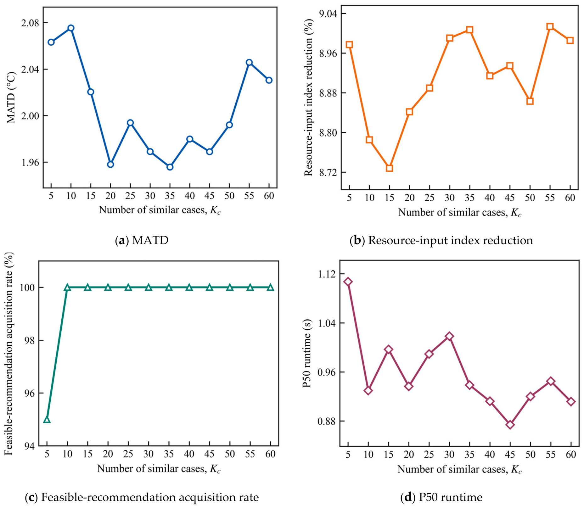
The number of similar cases, $K_c$, determines the range of local historical information used to establish the heat-specific reference level and initialize the population. To examine the influence of the retrieval range, $K_c$ was varied from 5 to 60 on 60 evenly spaced sampled heats using five identical random seeds, producing 12 parameter settings and 3600 optimization tasks. All settings used the same search budget and were run in randomized interleaved order after warm-up to reduce batch effects in runtime comparisons. The results are presented in Figure 6.

Figure 6 shows that the feasible-recommendation acquisition rate is 95.00% at $K_c$ = 5, indicating that an excessively narrow case neighborhood cannot provide a stable reference level and initialization information for a small number of heats. All tasks obtain feasible recommendations when $K_c$ ≥ 10. MATD remains between 1.956 and 1.994 °C for $K_c$ = 20–50, while the resource-input index reduction ranges from 8.84% to 9.01%, forming a stable performance region. $K_c$ = 35 provides a favorable combination of MATD, resource-input index reduction, and runtime and is therefore selected as the baseline for the main experiment and algorithm comparison. Except at $K_c$ = 5, P50 runtime ranges from 0.874 to 1.018 s and does not increase systematically with the number of retrieved cases, indicating that the additional computational cost of a wider retrieval range is small for the present case-base size and fixed search budget.

To distinguish the influence of historical case utilization intensity from that of local-search frequency, the case-initialization ratio ${\rho }_c$ and local-search interval $G_L$ were varied separately on the same 60 evenly spaced sampled heats and five random seeds, while all other parameters were held constant. The results are presented in

Table 12. Sensitivity results for the case-initialization ratio and local-search interval.

Parameter	Value	MATD (°C)	Resource-Input Index Reduction (%)	Feasible-Recommendation Acquisition Rate (%)	P50 Runtime (s)
${\rho }_c$	0.25	1.970	8.84	100.00	0.988
${\rho }_c$	0.50	1.956	9.01	100.00	0.930
${\rho }_c$	0.75	1.963	8.91	100.00	1.050
$G_L$	5	1.986	8.92	100.00	1.238
$G_L$	10	1.956	9.01	100.00	0.930
$G_L$	20	1.977	8.99	100.00	0.951

.

All parameter settings in Table 12 achieve a 100% feasible-recommendation acquisition rate. When ${\rho }_c$ increases from 0.25 to 0.50 and 0.75, the MATD values are 1.970, 1.956, and 1.963 °C; the resource-input index reductions are 8.84%, 9.01%, and 8.91%; and the P50 runtimes are 0.988, 0.930, and 1.050 s, respectively. Thus, ${\rho }_c$ = 0.50 performs favorably on all three metrics. For $G_L$ values of 5, 10, and 20, the MATD values are 1.986, 1.956, and 1.977 °C; the resource-input index reductions are 8.92%, 9.01%, and 8.99%; and the P50 runtimes are 1.238, 0.930, and 0.951 s, respectively. Among the three tested levels, $G_L$ = 10 simultaneously yields the lowest MATD, the largest resource-input index reduction, and a short runtime. The baseline settings ${\rho }_c$ = 0.50 and $G_L$ = 10 therefore balance search quality, population diversity, and computational efficiency.

4.2.3. Convergence and Stability of the Hybrid Algorithm

To analyze the effects of case initialization and tabu search, standard GA, GA with case initialization, GA with tabu search, and the complete method were compared on 20 evenly spaced sampled heats using 10 identical random seeds. Differential evolution (DE) was included as a population-based reference algorithm using the best/1/bin strategy, a mutation factor of 0.5–1.0, a crossover probability of 0.70, 24 individuals, and 120 generations, without terminal local refinement. All algorithms used the same heats, random seeds, prediction-model interfaces, hard constraints, and maximum number of generations.

Using one candidate scheme evaluated through the complete endpoint-model interface as the common counting unit, standard GA and GA with case initialization require approximately 2.4 × 10³ candidate evaluations for a complete 120-generation run. The methods incorporating tabu search require up to approximately 5.9 × 10³ evaluations under the settings of 12 local-search triggers, two elite solutions per trigger, at most six local iterations per elite, and 24 neighborhood candidates per iteration. DE with a population size of 24 requires approximately 2.9 × 10³ evaluations. If the no-improvement termination criterion is triggered early, the actual number of evaluations will be lower than these upper bounds. Candidate evaluation budget, solution quality, G95, and runtime are considered jointly in the following discussion.

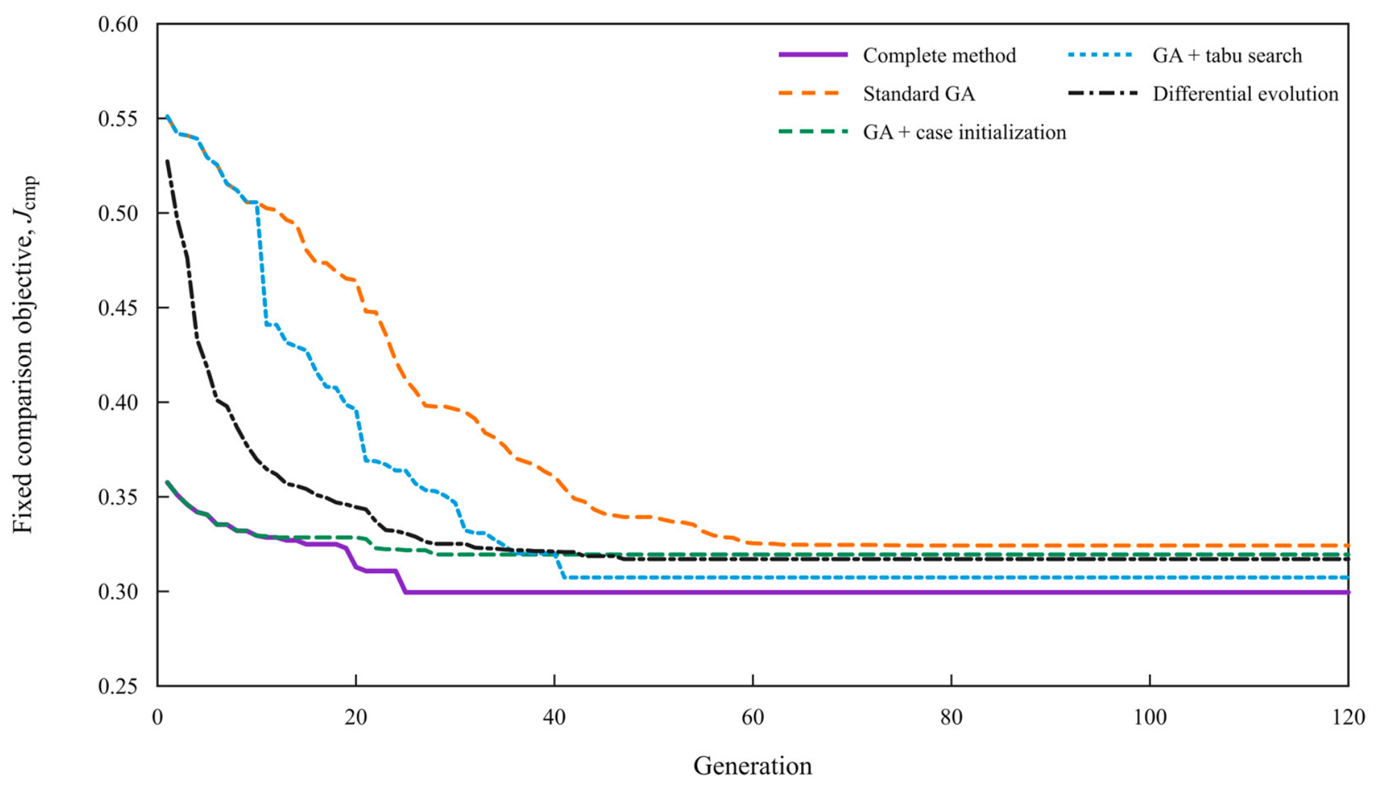
Because the dynamic weights make search-objective values from different generations incomparable, all feasible candidates in each generation were re-evaluated using a common comparison index with equal 50% contributions from the temperature-error and resource-input terms, and the best value obtained up to each generation was recorded. This index is used only to compare convergence on a common scale and does not participate in individual selection or termination. Figure 7 presents the median trajectories over 200 runs, and

Table 13. Results of repeated algorithm runs.

Algorithm	MATD (°C)	Resource-Input Index Reduction (%, Mean ± SD)	Feasible-Recommendation Acquisition Rate (%)	Runtime P50 (s)	Runtime P95 (s)
Standard GA	1.858	7.86 ± 3.01	100.00	1.509	2.203
GA + case initialization	1.837	7.90 ± 2.95	100.00	0.618	1.867
GA + tabu search	1.823	7.96 ± 2.73	100.00	1.468	2.381
Complete method	1.819	8.01 ± 1.85	100.00	0.814	1.873
DE	2.069	8.08 ± 2.39	100.00	5.081	7.251

summarizes MATD, resource-input index reduction, feasible-recommendation acquisition rate, and runtime for the five algorithms. P50 and P95 are the 50th and 95th percentiles, respectively, of the 200-run runtime distribution. G95 is defined as the earliest generation at which 95% of the total decrease from the first-generation value to the final value of the common comparison index has been achieved.

Figure 7 shows that GA with case initialization and the complete method both begin at 0.358, which is 35.1% lower than the initial value of 0.551 for standard GA and GA with tabu search. Similar cases therefore guide the initial population toward a better search region. As iteration proceeds, standard GA, GA with case initialization, GA with tabu search, the complete method, and DE converge to final index values of 0.324, 0.320, 0.307, 0.300, and 0.317, respectively. Relative to standard GA, tabu search reduces the final index from 0.324 to 0.307; adding tabu search to case initialization further reduces it from 0.320 to 0.300. The complete method consequently achieves the lowest final index among the five algorithms, indicating that case guidance and local refinement are complementary. The corresponding G_95 values are 54, 28, 41, 25, and 27 generations. Case initialization shortens G_95 from 54 to 28 generations, tabu search shortens it to 41 generations, and their combination further reduces it to 25 generations and produces a stable plateau after approximately generation 25. Thus, case initialization primarily improves the starting point and early search efficiency, whereas tabu search improves solution quality during the middle and late stages; together, they produce the fastest principal improvement and the best final result.

Table 13 shows that all 200 repeated runs of each of the five algorithms yield recommendations satisfying the prescribed model constraints. The complete method achieves a MATD of 1.819 °C, a mean resource-input index reduction of 8.01%, and a standard deviation of 1.85 percentage points. Relative to standard GA, it lowers MATD by 0.039 °C and increases the resource-input index reduction by 0.15 percentage points. Relative to GA with case initialization, the improvements are 0.018 °C and 0.11 percentage points, while relative to GA with tabu search, they are 0.004 °C and 0.05 percentage points. The complete method achieves both the lowest MATD and the largest resource-input index reduction among the four genetic variants, together with the smallest standard deviation of resource-input index reduction, indicating that the combination of case initialization and tabu search improves both solution quality and repeated-run stability. DE yields a resource-input index reduction of 8.08%, 0.07 percentage points higher than that of the complete method, but its MATD increases to 2.069 °C, 0.250 °C above that of the complete method; thus, its additional resource reduction is accompanied by a larger target-temperature deviation. In terms of computational efficiency, the complete method has P50 and P95 runtimes of 0.814 and 1.873 s, respectively. Relative to standard GA, these values are shorter by 46.1% and 15.0%; relative to GA with tabu search, they are shorter by 44.6% and 21.3%; and relative to DE, they are shorter by 84.0% and 74.2%. GA with case initialization has the shortest P50 runtime of 0.618 s, but its final common comparison index and the temperature–resource results in Table 13 are inferior to those of the complete method. Compared with that algorithm, the complete method increases P50 by 31.7% and P95 by only 0.3%. Together with Figure 7, these results show that case initialization reduces the computation required to enter a high-quality region and offsets part of the cost of tabu local search, enabling the complete method to retain per-heat runtimes on the order of seconds while achieving the lowest common comparison index and a favorable temperature–resource balance.

To further examine the paired differences between the complete method and GA + case initialization, GA + tabu search, and DE, the mean paired differences in MATD and resource-input index reduction, their 95% bias-corrected and accelerated (BCa) confidence intervals obtained from 50,000 heat-level bootstrap resamples, the results of two-sided exact Wilcoxon signed-rank tests with Holm correction for the three comparisons, and the rank-biserial effect sizes are summarized in

Table 14. Heat-level paired statistical comparisons between the complete method and reference algorithms.

Metric	Comparator	Mean Paired Difference (Comparison with the Complete Method)	95% BCa CI	Holm-Adjusted Wilcoxon p-Value	Rank-Biserial Effect Size
MATD	GA + case initialization	−0.018	[−0.032, −0.007]	0.0306	−0.610
MATD	GA + tabu search	−0.004	[−0.016, 0.012]	0.5706	−0.152
MATD	DE	−0.250	[−0.311, −0.186]	<0.001	−0.990
Resource-input index reduction	GA + case initialization	+0.110	[−0.077, 0.274]	0.6073	+0.333
Resource-input index reduction	GA + tabu search	+0.050	[−0.069, 0.172]	0.7768	+0.190
Resource-input index reduction	DE	−0.070	[−0.198, 0.057]	0.7768	−0.229

. Specifically, the 10 random-seed results obtained by each algorithm for each heat were first averaged, and the subsequent analyses were conducted using the resulting 20 heat-level means.

Table 14 further clarifies the statistical and practical significance of the performance differences summarized in Table 13. Compared with GA + case initialization, the complete method reduced the MATD by 0.018 °C. Its 95% BCa confidence interval lay entirely below zero, and the difference remained statistically significant after Holm correction (p = 0.0306), with a rank-biserial effect size of −0.610. This result indicates that the incorporation of tabu search produced a modest improvement in temperature-control error, with a relatively consistent direction across the evaluated heats. By contrast, the differences between the complete method and GA + tabu search were only −0.004 °C for MATD and +0.050 percentage points for resource-input index reduction. Both confidence intervals crossed zero, and both Holm-adjusted p-values were greater than 0.05. Therefore, within the scope of the present experiments, the primary contribution of case initialization was reflected in improved search efficiency, including a lower initial unified comparison metric, a smaller G95, and shorter P50 and P95 runtimes, while also providing feasible baseline candidate solutions for the subsequent search. Furthermore, compared with DE, the complete method reduced the MATD by 0.250 °C. The corresponding confidence interval lay entirely below zero, the Holm-adjusted p-value was less than 0.001, and the rank-biserial effect size was −0.990. Although the resource-input index reduction achieved by DE was 0.070 percentage points greater than that achieved by the complete method, this difference was not statistically significant. These results further demonstrate that the complete method achieved a favorable combination of MATD and resource-input index reduction while maintaining a good overall balance among temperature-control performance, convergence behavior, and computational efficiency.

5. Conclusions

(1)

A collaborative LF operating-parameter optimization method based on prediction models and case-guided genetic–tabu search was developed within a prediction–optimization control framework. The normalized temperature-deviation and resource-input index terms were combined in a unified objective, and the weights were dynamically adjusted by coupling generational annealing with feasible-population temperature-error feedback. Endpoint temperature, S, Mn, Als, O, operating ranges, and the historical operating-condition support domain were imposed as hard constraints. Similar qualified heats were used consistently for heat-specific reference-index calculation, support-domain construction, and population initialization, linking case retrieval, candidate evaluation, and optimization.

(2)

For the 400 independent evaluation heats, every optimized recommendation satisfied the hard constraints. Relative to the historical operations, the mean recommended quantities of lime, slag agent, aluminum granules, and high-carbon ferromanganese decreased by 6.98%, 12.79%, 9.34%, and 8.85%, respectively, while electric energy input and power-on duration decreased by 7.89% and 8.95%. The 95% BCa confidence intervals for all six per-heat reductions lay above zero, and all Holm-adjusted p-values were below 0.001. Error-margin experiments for the temperature, S, Mn, O, and Als interfaces yielded feasible recommendations for 96.25% and 93.25% of heats at margins of 0.25 × MAE and 0.50 × MAE, respectively, while retaining resource-input index re-ductions of 8.45% and 8.15%.

(3)

Extended sensitivity experiments showed that the overall temperature–resource trade-off remained stable as the number of similar cases, case-initialization ratio, local-search interval, and resource coefficients varied within the tested ranges. Algorithm comparison further demonstrated that case initialization markedly improved the starting point of the search and that tabu search strengthened local exploitation during the middle and late stages. Across 20 heats and 10 random seeds, the complete method achieved a MATD of 1.819 °C, a resource-input index reduction of 8.01%, and a 100% feasible-recommendation acquisition rate, with P50 and P95 runtimes of 0.814 and 1.873 s per heat, respectively. These results indicate a favorable overall balance among temperature control, resource reduction, and computational efficiency.

(4)

The quantitative results apply to SPHC steel from the investigated LF line within its historical data support domain. The objective organization, candidate-evaluation interface, case-guidance mechanism, and genetic–tabu hybrid search workflow can be transferred to other metallurgical settings; however, transfer to another grade, ladle condition, furnace capacity, or process route requires the endpoint-prediction models, operating bounds, case-base statistics, retrieval weights, support-domain threshold, resource coefficients, and necessary search parameters to be rebuilt or recalibrated using chronologically separated data from the target line. Before online deployment, prospective heats should be used to evaluate actual resource savings, endpoint-quality stability, abnormal-condition handling, and operational safety.

References

1. Zhang, R.H.; Yang, J. State of the art in applications of machine learning in steelmaking process modeling. Int. J. Miner. Metall. Mater. 2023, 30, 2055–2075. [Google Scholar] [CrossRef] [Scilit]
2. Pepe, C.; Farella, G.; Bartucci, G.; Zanoli, S.M. Recent innovations in computer and automation engineering for performance improvement in the steel industry production chain: A review. Energies 2025, 18, 1981. [Google Scholar] [CrossRef] [Scilit]
3. Guo, X.P.; Ryan, S.; Walla, N.; Zhou, C. Numerical simulation of electric arc heating process in the refining ladle. Steel Res. Int. 2023, 94, 2300195. [Google Scholar] [CrossRef] [Scilit]
4. Makela, I.; Visuri, V.V.; Fabritius, T. A mathematical model for the thermal state of a steel ladle. Ironmak. Steelmak. 2023, 50, 867–877. [Google Scholar] [CrossRef] [Scilit]
5. Song, J.; Zhang, J.M.; Yin, Y.B.; Zhen, X.-G. Optimizing power-saving process for a 120-t ladle furnace. J. Iron Steel Res. Int. 2025, 32, 594–605. [Google Scholar] [CrossRef] [Scilit]
6. Guo, J.W.; Zhan, D.P.; Xu, G.C.; Yang, N.-H.; Wang, B.; Wang, M.-X.; You, G.-W. An online BOF terminal temperature control model based on big data learning. J. Iron Steel Res. Int. 2023, 30, 875–886. [Google Scholar] [CrossRef] [Scilit]
7. Beden, S.; Lakshmanan, K.; Giannetti, C.; Beckmann, A. Steelmaking predictive analytics based on random forest and semantic reasoning. Appl. Sci. 2023, 13, 12778. [Google Scholar] [CrossRef] [Scilit]
8. Dong, Q.Q.; Li, M.; Hu, S.J.; Yu, Y.; Gu, M. Multi-output prediction model for basic oxygen furnace steelmaking based on the fusion of deep convolution and attention mechanisms. Metals 2024, 14, 773. [Google Scholar] [CrossRef] [Scilit]
9. Choi, S.W.; Seo, B.G.; Lee, E.B. Machine learning-based tap temperature prediction and control for optimized power consumption in stainless electric arc furnaces (EAF) of steel plants. Sustainability 2023, 15, 6393. [Google Scholar] [CrossRef] [Scilit]
10. Yang, J.P.; Zhang, J.S.; Guo, W.D.; Gao, S.; Liu, Q. End-point temperature preset of molten steel in the final refining unit based on an integration of deep neural network and multi-process operation simulation. ISIJ Int. 2021, 61, 2100–2110. [Google Scholar] [CrossRef] [Scilit]
11. Wang, X.J.; You, M.S.; Mao, Z.Z.; Yuan, P. Tree-structure ensemble general regression neural networks applied to predict the molten steel temperature in ladle furnace. Adv. Eng. Inform. 2016, 30, 368–375. [Google Scholar] [CrossRef] [Scilit]
12. Wang, X.J.; Yuan, P.; Mao, Z.Z.; You, M. Molten steel temperature prediction model based on bootstrap feature subsets ensemble regression trees. Knowl.-Based Syst. 2016, 101, 48–59. [Google Scholar] [CrossRef] [Scilit]
13. Wang, X.J. Ladle furnace temperature prediction model based on large-scale data with random forest. IEEE/CAA J. Autom. Sin. 2017, 4, 770–774. [Google Scholar] [CrossRef] [Scilit]
14. Feng, K.; He, D.F.; Xu, A.J.; Wang, H. End temperature prediction of molten steel in LF based on CBR-BBN. Steel Res. Int. 2016, 87, 79–86. [Google Scholar] [CrossRef] [Scilit]
15. Wang, X.J.; Wang, X.Y.; Zhang, Q.; Mao, Z.-Z. The soft sensor of the molten steel temperature using the modified maximum entropy based pruned bootstrap feature subsets ensemble method. Chem. Eng. Sci. 2018, 189, 401–412. [Google Scholar] [CrossRef] [Scilit]
16. Yang, Q.D.; Zhang, J.; Yi, Z. Predicting molten steel endpoint temperature using a feature-weighted model optimized by mutual learning cuckoo search. Appl. Soft Comput. 2019, 83, 105675. [Google Scholar] [CrossRef] [Scilit]
17. Yuan, F.; Xu, A.J.; Gu, M.Q. Development of an improved CBR model for predicting steel temperature in ladle furnace refining. Int. J. Miner. Metall. Mater. 2021, 28, 1321–1331. [Google Scholar] [CrossRef] [Scilit]
18. Qiao, Z.H.; Wang, B. Molten steel temperature prediction in ladle furnace using a dynamic ensemble for regression. IEEE Access 2021, 9, 18855–18866. [Google Scholar] [CrossRef] [Scilit]
19. Yang, Q.D.; Fu, Y.C.; Zhang, J. Molten steel temperature prediction using a hybrid model based on information interaction-enhanced cuckoo search. Neural Comput. Appl. 2021, 33, 6487–6509. [Google Scholar] [CrossRef] [Scilit]
20. Xin, Z.C.; Zhang, J.S.; Zheng, J.; Jin, Y.; Liu, Q. A hybrid modeling method based on expert control and deep neural network for temperature prediction of molten steel in LF. ISIJ Int. 2022, 62, 532–541. [Google Scholar] [CrossRef] [Scilit]
21. Wang, B.; Wang, W.J.; Meng, G.L.; Qiao, Z.; Guo, Y.; Wang, N.; Wang, W.; Mao, Z. Boosting the prediction of molten steel temperature in ladle furnace with a dynamic outlier ensemble. Eng. Appl. Artif. Intell. 2022, 116, 105359. [Google Scholar] [CrossRef] [Scilit]
22. Chen, C.; Wang, N.; Chen, M.; Yan, X. A framework based on heterogeneous ensemble models for liquid steel temperature prediction in LF refining process. Appl. Soft Comput. 2022, 131, 109724. [Google Scholar] [CrossRef] [Scilit]
23. Xin, Z.C.; Zhang, J.S.; Zhang, J.G.; Zheng, J.; Jin, Y.; Liu, Q. Predicting temperature of molten steel in LF-refining process using IF-ZCA-DNN model. Metall. Mater. Trans. B 2023, 54, 1181–1194. [Google Scholar] [CrossRef] [Scilit]
24. Feng, M.L.; Lin, L.; He, S.; Li, X.-C.; Hou, Z.-X.; Yao, T.-L. Temperature prediction model for ladle furnace based on mathematical mechanisms and the GA-BP algorithm. Ironmak. Steelmak. 2024, 51, 692–702. [Google Scholar] [CrossRef] [Scilit]
25. He, D.F.; Song, C.W.; Guo, Y.Z.; Feng, K. An error correction method based on CBR for end temperature prediction of molten steel in ladle furnace. ISIJ Int. 2024, 64, 1291–1300. [Google Scholar] [CrossRef] [Scilit]
26. Xin, Z.C.; Zhang, J.S.; Peng, K.X.; Zhang, J.; Zhang, C.; Wu, J.; Zhang, B.; Liu, Q. Explainable machine learning model for predicting molten steel temperature in the LF refining process. Int. J. Miner. Metall. Mater. 2024, 31, 2657–2669. [Google Scholar] [CrossRef] [Scilit]
27. Wang, H.; Wang, M.; Liu, Q.; Yang, Z.; Xing, L. Prediction of ladle furnace refining endpoint temperature based on particle swarm optimization algorithm and long short-term memory neural network. JOM 2025, 77, 282–293. [Google Scholar] [CrossRef] [Scilit]
28. Li, X.L.; He, D.F.; Guo, Y.Z.; Feng, K. Improvement in stability and generalization ability of end-point temperature prediction model in ladle furnace. J. Sustain. Metall. 2025, 11, 4347–4363. [Google Scholar] [CrossRef] [Scilit]
29. Kavic, D.; Bernhard, M.; Rossler, R.; Schalk, L.; Bernhard, C. Enhanced temperature prediction in ladle furnace steel refining: Hybrid process modeling based on computational thermodynamics and statistical learning methods. Metall. Mater. Trans. B 2025, 56, 5682–5699. [Google Scholar] [CrossRef] [Scilit]
30. Andreiana, D.S.; Acevedo Galicia, L.E.; Ollila, S.; Guerrero, C.L.; Roldán, Á.O.; Navas, F.D.; Torres, A.d.R. Steelmaking process optimised through a decision support system aided by self-learning machine learning. Processes 2022, 10, 434. [Google Scholar] [CrossRef] [Scilit]
31. Shi, C.Y.; Wang, B.S.; Guo, S.Y.; Yin, X.X.; Wang, Y.K.; Zhang, L.; Chen, R.; Ma, Z.C. Prediction of alloy addition in ladle furnace (LF) based on LWOA-SCN. Metalurgija 2023, 62, 359–362. [Google Scholar]
32. Xin, Z.C.; Zhang, J.S.; Jin, Y.; Zheng, J.; Liu, Q. Predicting the alloying element yield in a ladle furnace using principal component analysis and deep neural network. Int. J. Miner. Metall. Mater. 2023, 30, 335–344. [Google Scholar] [CrossRef] [Scilit]
33. Kothari, A.K.; Ranjan, R.; Singh, R.S.; Kumar, G.; Kumar, A.; Agrawal, A. A real-time ferroalloy model for the optimum ladle furnace treatment during the secondary steelmaking. Ironmak. Steelmak. 2019, 46, 211–220. [Google Scholar] [CrossRef] [Scilit]
34. Regulski, K.; Rauch, L.; Hajder, P.; Bzowski, K.; Opaliński, A.; Pernach, M.; Hallo, F.; Piwowarczyk, M.; Kalinowski, S. Optimizing continuous casting through cyber-physical system. Processes 2024, 12, 1761. [Google Scholar] [CrossRef] [Scilit]
35. Jawahery, S.; Visuri, V.V.; Wasbo, S.O.; Hammervold, A.; Hyttinen, N.; Schlautmann, M. Thermophysical model for online optimization and control of the electric arc furnace. Metals 2021, 11, 1587. [Google Scholar] [CrossRef] [Scilit]
36. Tian, H.X.; Liu, Y.D.; Li, K.; Yang, R.-R.; Meng, B. A new AdaBoost.IR soft sensor method for robust operation optimization of ladle furnace refining. ISIJ Int. 2017, 57, 841–850. [Google Scholar] [CrossRef] [Scilit]
37. Kannisto, P.; Kargar, Z.; Alvarez, G.; Kleimt, B.; Arteaga, A. Resilient, adaptive industrial Self-X AI pipeline with external AI services: A case study on electric steelmaking. Processes 2024, 12, 2877. [Google Scholar] [CrossRef] [Scilit]
38. Saadi, F.; Atmani, B.; Henni, F. Improving retrieval performance of case based reasoning systems by fuzzy clustering. Int. J. Interact. Multimed. Artif. Intell. 2024, 9, 84–91. [Google Scholar] [CrossRef] [Scilit]
39. Chen, Z.H.; Xu, X.C.; Liu, H.B. Improved dual-population genetic algorithm: A straightforward optimizer applied to engineering optimization. Sustainability 2023, 15, 14821. [Google Scholar] [CrossRef] [Scilit]
40. Dutta, S.; Mallipeddi, R.; Das, K.N. Hybrid selection based multi/many-objective evolutionary algorithm. Sci. Rep. 2022, 12, 6861. [Google Scholar] [CrossRef] [Scilit] [PubMed]
41. Sakabe, M.; Yagiura, M. An efficient tabu search algorithm for the linear ordering problem. J. Adv. Mech. Des. Syst. Manuf. 2022, 16, JAMDSM0041. [Google Scholar] [CrossRef] [Scilit]
42. Lai, X.; Lin, Z.; Hao, J.K.; Wu, Q. An efficient optimization model and tabu search-based global optimization approach for the continuous p-dispersion problem. INFORMS J. Comput. 2025, 37, 1018–1043. [Google Scholar] [CrossRef] [Scilit]
Figure 1. Workflow of the prediction–optimization control model.
Processes 14 02994 g001
Figure 3. Mean reductions in recommended operating quantities relative to historical operation.
Processes 14 02994 g003
Figure 4. Per-heat distributions of operating-quantity reductions among the 400 feasible recommendations: (a) Lime. (b) Slag agent. (c) Aluminum granules. (d) High-carbon ferromanganese. (e) Electric energy input. (f) Power-on duration. The red solid line indicates the median, the box spans the interquartile range (IQR), and the dots denote observations lying more than 1.5 times the IQR below the first quartile or above the third quartile.
Processes 14 02994 g004
Figure 5. Dynamic temperature-weight trajectories for 10 representative heats. The different colors are used only to distinguish the temperature-weight trajectories of the 10 representative heats and do not represent additional process categories.
Processes 14 02994 g005
Figure 6. Effects of the number of similar cases on: (a) MATD; (b) resource-input index reduction; (c) feasible-recommendation acquisition rate; (d) P50 runtime.
Processes 14 02994 g006
Figure 7. Median convergence trajectories of the common comparison index with 50% temperature-error and 50% resource terms for five algorithms.
Processes 14 02994 g007