An Analytical Method for Estimating Large-Scale Cave Volume in Fractured-Vuggy Carbonate Reservoirs of the Tarim Basin, China

Abstract

Large-scale caves provide important storage space in carbonate oil and gas reservoirs. However, accurately estimating their volume remains challenging because of complex geometries and limited access to underground cavities. In this study, an analytical well-test method is proposed to estimate large-scale cave volume from pressure-transient responses. A physical model is first established and mathematically formulated, followed by the derivation of an analytical solution in the Laplace domain. Stehfest’s numerical inversion is then applied to obtain pressure and pressure-derivative-type curves under different outer boundary conditions. The results identify four characteristic flow regimes: the wellbore-storage regime, the transition-flow regime, the cave-storage regime, and the boundary-dominated flow regime. A distinct concave feature is observed in the pressure-derivative curves. Sensitivity analysis shows that the pressure response is mainly influenced by three dimensionless parameters: the depth coefficient, radius coefficient, and shape coefficient. The depth coefficient primarily determines the transition time of the wellbore-storage regime, the radius coefficient mainly affects the width and depth of the concave response, and the shape coefficient mainly influences its magnitude. Finally, two field cases are presented to demonstrate the applicability of the proposed method for estimating cave volume.

1. Introduction

Large-scale caves represent important storage spaces in fractured-vuggy carbonate reservoirs and are particularly common in the western regions of China. These cavities may originate from natural geological processes or be generated during reservoir stimulation operations, such as acidizing treatments. In terms of spatial structure, these caves usually exhibit irregular geometries, variable sizes, and complex connectivity with surrounding fractures, vugs and matrix pores. Temporally, prolonged geological evolution, including dissolution, collapse, filling, and fluid-rock interactions, may continuously modify cave geometry and storage capacity after their initial formation. Moreover, drilling operations may introduce additional uncertainties, including drill-string unloading and drilling-fluid losses, which may result in partial filling of the cavities [1]. The spatial distribution and temporal evolution of large-scale caves introduce significant uncertainties into reservoir characterization and make the accurate determination of cave volume challenging, particularly in deeply buried carbonate reservoirs where direct observation is extremely difficult.

Analytical well-test models remain valuable tools for investigating pressure-transient behavior and estimating reservoir parameters, particularly in complex carbonate reservoirs. In recent years, numerous analytical and semi-analytical models have been developed to describe fracture-cave systems with increasing geological complexity [2,3,4,5,6]. For fractured-caved carbonate reservoirs, Du et al. developed a generalized pressure and rate transient analysis model, in which Laplace-domain solutions were obtained for different cave configurations and characteristic flow regimes were analyzed using type curves [7].

Although considerable progress has been made, existing well-test models mainly focus on estimating effective reservoir properties, including permeability and interporosity-flow parameters, whereas direct evaluation of cave geometry remains limited. Several techniques have been developed to characterize underground cavities. Gravity-based methods can identify subsurface voids by analyzing gravity anomalies associated with density contrasts. Braitenberg et al. [8] investigated the feasibility of detecting karst caves using airborne and terrestrial gravity measurements based on a well-characterized cave system. However, these methods mainly provide information on cavity location and distribution, and their application to deeply buried carbonate reservoirs is restricted by resolution and accessibility. Moreover, electrical resistivity tomography and seismic refraction tomography have been combined to detect buried cavities by exploiting contrasts in electrical resistivity and seismic velocity between voids and host rocks [9]. However, these methods have limited accuracy for volume estimation, limited spatial resolution, and insufficient adaptability to complex cave geometries.

Direct measurement and three-dimensional reconstruction techniques have also been applied to cave characterization. Geological observations, sampling, and underground investigations have been used to analyze cave development and geometric evolution. For example, Van Hout et al. [10] proposed a methodology for evaluating cave evolution in mining environments through drawpoint sampling and geological observations. Recent advances in laser scanning and photogrammetric technologies have further enabled high-resolution reconstruction of complex cave structures. Fabbri et al. [11] demonstrated that terrestrial laser scanning (TLS) can generate centimeter-scale three-dimensional cave models and accurately quantify cave morphology and volume. Cazes et al. [12] integrated close-range photogrammetry and laser scanning to reconstruct full-scale cave structures and compared the accuracy of different three-dimensional modeling approaches. Zhang et al. [13] combined laser scanning and photogrammetry to establish high-precision real-scene three-dimensional models of karst cave landscapes, achieving improved geometric completeness through multi-source data fusion. Nevertheless, these direct measurement approaches generally require physical access to the cave environment and are therefore mainly applicable to exposed or shallow caves. Their application to deeply buried fractured-vuggy carbonate reservoirs remains highly challenging.

For subsurface carbonate reservoirs, dynamic-response methods provide an alternative approach to evaluating cave characteristics. Chen et al. [14] developed a pressure-transient model for fractured-vuggy carbonate reservoirs containing large-scale caves by incorporating cave-storage effects into well-test analysis. Their results indicated that pressure-derivative characteristics can be used to identify cave-related flow behavior. However, the model only infers the location and size of large-scale caves and cannot directly calculate cave volume. Wan et al. [15] further established a numerical well-test model for caved carbonate reservoirs and analyzed the effects of cave size, location, and connectivity on pressure responses; however, the model characterizes caves through simplified geometric assumptions and cannot directly estimate the actual cave volume. Li et al. [16] proposed a well-test model for fractured-vuggy carbonate reservoirs with a vertical bead-on-a-string structure and introduced a dimensionless cave storage parameter to characterize cave-storage effects. However, the authors acknowledged that no field data were available to accurately describe cave locations and volumes at that time, and the proposed model still requires further field validation. In addition, Yue et al. [17] used water-injection curves to evaluate the dynamic behavior of fractured-vuggy carbonate reservoirs and estimated the effective storage capacity. This approach can estimate cave volume, but it relies on long-term production data, which limits its applicability to rapid evaluation of newly drilled wells. Therefore, an effective methodology that can quantitatively estimate the volume of irregular large-scale caves while accounting for reservoir dynamic responses is still required.

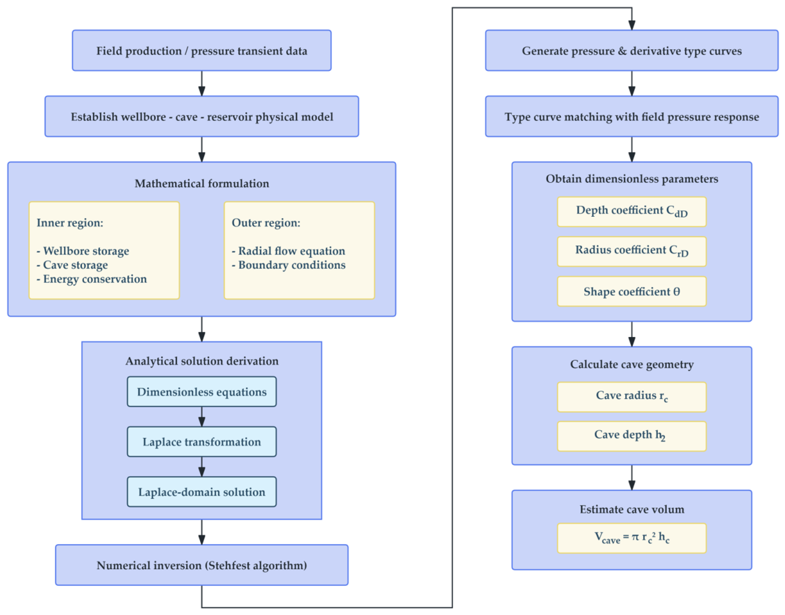
Based on these observations, a new method is needed to determine large-scale cave volume. The main objective of this study is to propose an analytical well-testing model that can meet this requirement. The proposed model is first established based on the physical characteristics of cave-containing reservoirs, and the governing equations are subsequently converted into dimensionless forms. Analytical solutions under different outer boundary conditions are derived through Laplace transformation. Using numerical inversion techniques, pressure and pressure-derivative-type curves are generated to identify characteristic flow regimes and analyze the effects of key model parameters. Finally, two field cases are presented to demonstrate the applicability of the proposed approach for quantitative cave-volume estimation. Figure 1 illustrates the workflow of the proposed analytical method for estimating large-scale cave volume.

2. Materials and Methods

2.1. Geographical and Geological Setting

The Tarim Basin, located in northwestern China, is a large intracratonic basin surrounded by the Tianshan, Kunlun, and Altun Mountains. Thick marine carbonate successions were widely deposited from the Cambrian to the Middle Ordovician, providing an important geological foundation for carbonate reservoir development. Since the Middle-Late Ordovician, the basin has experienced multiple stages of tectonic deformation, regional uplift, erosion, and unconformity development. Extensive fault systems developed in major structural zones, particularly in the Tabei and Tazhong areas. These tectonic structures provided preferential pathways for fluid migration and played an important role in controlling the distribution and development of subsequent paleokarst systems.

The Ordovician carbonate successions subsequently underwent prolonged dissolution and karstification, resulting in complex and strongly heterogeneous reservoir spaces. These processes generated multiscale storage and flow units, including fractures, vugs, dissolution pores, and large-scale caves. Fault zones are closely associated with the development and distribution of these karst-related reservoir spaces because they facilitate fluid circulation and enhance dissolution [18]. Consequently, the Ordovician carbonate reservoirs of the Tarim Basin are characterized by deep burial, complex tectonic modification, multiscale reservoir architecture, and strong spatial heterogeneity.

The geological framework provides an important basis for investigating the dynamic behavior of large-scale caves. In particular, the coexistence of fractures, vugs, and caves produces strong spatial variability in storage capacity and fluid-flow pathways. Therefore, a geological description that accounts for the formation and distribution of these reservoir spaces is essential for establishing a model to quantitatively interpret the pressure response associated with large-scale cave storage.

2.2. Geological Model and Petrophysical Characteristics

Fractured-vuggy carbonate reservoirs contain multiple types of reservoir spaces, including rock matrix, fractures, vugs, dissolution pores, and large-scale caves. The characteristic dimensions and geometries of these storage spaces can vary over several orders of magnitude. Large-scale dissolution caves may have irregular shapes and characteristic diameters ranging from several tens of millimeters to several tens of meters [19]. The coexistence of reservoir spaces with substantially different scales results in diverse fracture-vug-cave configurations and complex connectivity relationships within the reservoir. Accordingly, fluid flow may occur through different mechanisms and at different spatial scales, ranging from Darcy flow in the matrix to relatively free flow in larger caves and fractures. Under some conditions, the flow regime may also vary from predominantly laminar flow in small-scale porous spaces to more complex local flow in larger conduits [20].

A distinctive petrophysical characteristic of fractured-vuggy carbonate reservoirs is the extremely low matrix porosity and permeability. Statistical analysis of approximately 2000 core samples from the Tahe Oilfield showed that matrix porosity ranges from 0.06% to 1.3%, with an average value of 0.62%, and that 92.9% of the samples have porosity below 1%. Matrix permeability ranges from 0.001 to 1.97 mD, with an average value of 0.066 mD, and approximately 80% of the samples have permeability below 0.1 mD [21]. These characteristics indicate that the matrix has limited flow capacity, whereas well-developed fractures generally provide substantially more effective pathways for fluid migration. Consequently, fractures can act as preferential flow channels and may establish hydraulic communication between different vugs and caves.

The present-day geological architecture of these reservoirs results from multiple stages of geological evolution, including superimposed karstification, hydrocarbon accumulation, and repeated tectonic deformation [22]. As a result, fractures and dissolution-related cavities are distributed heterogeneously, with variable geometries, sizes, and connectivity. Large-scale caves and fractures may occur as discrete, spatially separated bodies, and different fracture-vug-cave assemblages may be associated with different fluid contacts and pressure systems [21]. In addition, large-scale caves may undergo post-formational modification through physical and chemical processes. Cave collapse and subsequent filling with unconsolidated materials, such as gravel, sand, and mud, can reduce effective void space and alter the storage and flow characteristics of the cavity [23,24].

These geological and petrophysical characteristics make direct characterization of large-scale cave volume particularly challenging. Strong reservoir heterogeneity, a broad range of spatial scales, irregular cave geometries, variable connectivity, and post-formational modification introduce substantial uncertainty into the determination of effective cave size and storage capacity. Therefore, the geological model considered in this study focuses on the dominant storage and flow characteristics of a large-scale cave and its surrounding formation, rather than attempting to reproduce the detailed three-dimensional geometry of an individual natural cave.

2.3. Physical Model and Assumptions

Given the complex geological and petrophysical characteristics described above, a simplified physical model is established to investigate the dominant pressure-transient response associated with large-scale cave storage while maintaining analytical tractability. The purpose of this simplification is to establish a quantitative relationship between the storage and geometric characteristics of the cave and the pressure response observed at the wellbore. The detailed three-dimensional heterogeneity, irregular cave geometry, and complex fracture-cave connectivity of natural reservoirs are therefore not explicitly reproduced in the analytical model.

To ensure that the problem is tractable, the following assumptions are adopted:

(1)

The large-scale cave is cylindrical and concentric with the wellbore.

(2)

The formation is isotropic and cylindrical. A well is located at the center of the formation and produces at a constant surface flow rate q, where Bq represents the corresponding reservoir-condition volumetric flow rate.

(3)

Formation properties, such as permeability, thickness, and porosity, are constant.

(4)

We consider single-phase compressible oil. The compressibility and viscosity of the oil are also assumed constant.

(5)

Gravity and capillary effects are neglected.

(6)

The reservoir pressure in every site is uniform and equal to p_i.

(7)

The fluid flow in the formation obeys Darcy’s law and is isothermal.

It should be noted that the cylindrical and concentric representation provides a simplified geometric description of the cave that enables an analytical solution to be derived while retaining the principal storage effect of the cavity. The model also introduces a shape coefficient to approximately account for deviations of the actual cave geometry from the ideal cylindrical configuration. Consequently, the proposed framework is intended to capture the dominant pressure-transient characteristics associated with large-scale cave storage rather than reproduce the detailed three-dimensional geometry of individual natural caves.

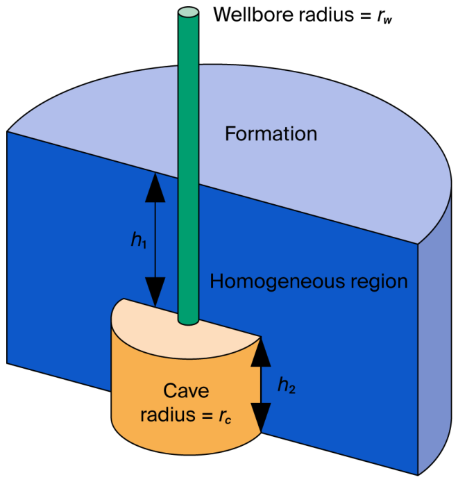
Based on the above assumptions, the physical model is shown in Figure 2. In this work, the reservoirs are divided into two sections. The inner region is the wellbore and the large-scale cave. The wellbore is connected to the cave, and the radii of the wellbore and the cave are r_w and r_c; the depths of the wellbore and cave are h₁ and h₂, respectively. For clarity, h₁ and h₂ are also explicitly labeled in Figure 3. The outer region is the formation, which is regarded as a homogeneous region, and the permeability, porosity, and compressibility are k, $\varphi$, and c_t.

3. Mathematical Model

In this section, the governing equations and their solutions are presented. The equations are first transformed into dimensionless forms, and the Laplace transformation is then applied to derive the pressure solution in the Laplace domain.

3.1. Governing Equations

For most well-test models, the following continuity and momentum conservation equations are considered:

$${\displaystyle \frac{\partial \rho }{\partial t}}+{\displaystyle \frac{\partial }{\partial x}}(\rho v)=0$$

(1)

$$\rho \left({\displaystyle \frac{\partial v}{\partial t}}+v{\displaystyle \frac{\partial v}{\partial x}}\right)+{\displaystyle \frac{\partial p}{\partial x}}=0$$

(2)

where t is the time, ρ represents the density of the fluid, and v denotes the velocity.

Expanding Equations (1) and (2) gives

$${\displaystyle \frac{\partial \rho }{\partial t}}+v{\displaystyle \frac{\partial \rho }{\partial x}}+\rho {\displaystyle \frac{\partial v}{\partial x}}=0$$

(3)

$$\rho {\displaystyle \frac{\partial v}{\partial t}}+\rho v{\displaystyle \frac{\partial v}{\partial x}}+{\displaystyle \frac{\partial p}{\partial x}}=0$$

(4)

Multiplying Equation (3) by $v$, we obtain

$$v{\displaystyle \frac{\partial \rho }{\partial t}}+v^2{\displaystyle \frac{\partial \rho }{\partial x}}+\rho v{\displaystyle \frac{\partial v}{\partial x}}=0$$

(5)

Adding Equations (4) and (5), we obtain

$$\rho {\displaystyle \frac{\partial v}{\partial t}}+v{\displaystyle \frac{\partial \rho }{\partial t}}+v^2{\displaystyle \frac{\partial \rho }{\partial x}}+2\rho v{\displaystyle \frac{\partial v}{\partial x}}+{\displaystyle \frac{\partial p}{\partial x}}=0$$

(6)

We know that

$$\rho {\displaystyle \frac{\partial v}{\partial t}}+v{\displaystyle \frac{\partial \rho }{\partial t}}={\displaystyle \frac{\partial }{\partial t}}\left(\rho v\right)$$

(7)

$$v^2{\displaystyle \frac{\partial \rho }{\partial x}}+2\rho v{\displaystyle \frac{\partial v}{\partial x}}={\displaystyle \frac{\partial }{\partial x}}\left(\rho v^2\right)$$

(8)

Substituting Equations (7) and (8) into Equation (6) yields

$${\displaystyle \frac{\partial }{\partial t}}\left(\rho v\right)+{\displaystyle \frac{\partial }{\partial x}}\left(\rho v^2\right)+{\displaystyle \frac{\partial p}{\partial x}}=0$$

(9)

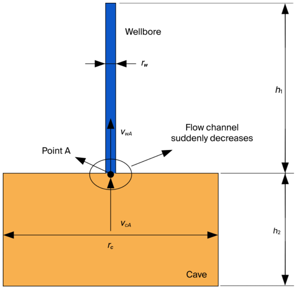
However, the energy conservation equation was not considered in previous studies, so the wellbore pressure $p_w$ is equal to the cave pressure $p_c$. In fact, the $r_c$ is much larger than the $r_w$. Therefore, when oil flows from the cave into the wellbore, the oil velocity changes drastically owing to the sudden decrease in the radius, as shown in Figure 3. This results in a pressure difference between $p_w$ and $p_c$, which is described as

$$p_c+{\displaystyle \frac{1}{2}}\rho v_{cA}^2=p_w+{\displaystyle \frac{1}{2}}\rho v_{wA}^2$$

(10)

where v_cA is the velocity of the fluid in the cave at point A, and v_wA is the velocity of the fluid in the wellbore at point A. We, therefore, have

$$\pi r_c^2{v}_{cA}=\pi r_w^2{v}_{wA}$$

(11)

because $r_c\gg r_w$, it follows that $v_{cA}\ll v_{wA}$. Therefore, the v_cA in Equation (10) can be neglected, yielding

$$p_c=p_w+{\displaystyle \frac{1}{2}}\rho v_{wA}^2$$

(12)

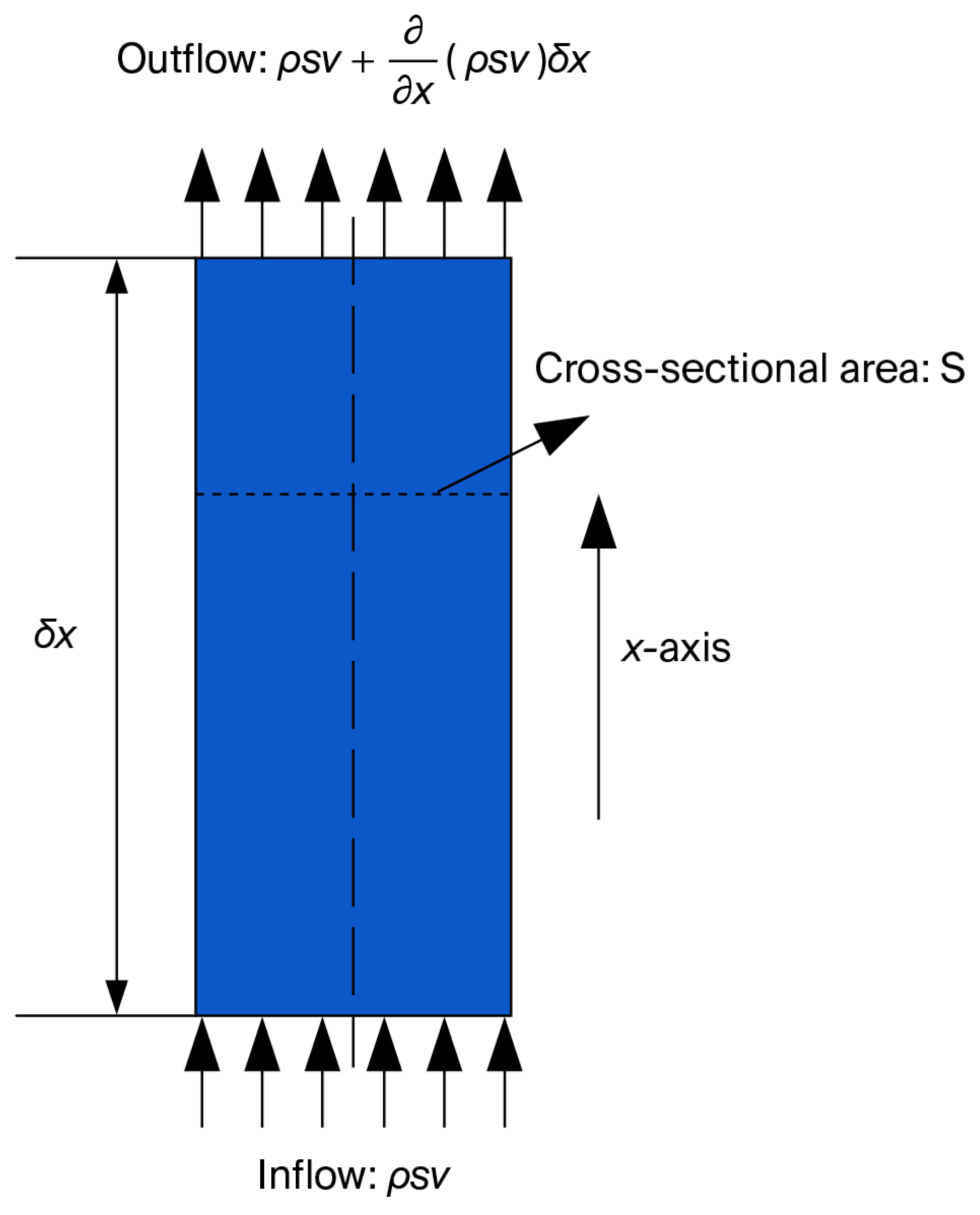
Therefore, we need to determine the expression for v_wA. As an example, consider an infinitesimal fluid element in the wellbore, as shown in Figure 4.

The mass conservation must be satisfied

$$\left[\rho sv+{\displaystyle \frac{\partial }{\partial x}}\left(\rho sv\right)\delta x\right]-\rho sv={\displaystyle \frac{\partial }{\partial t}}\left(\rho s\delta x\right)$$

(13)

where s is the cross-sectional area of the infinitesimal, and

$$s=\pi r_w^2$$

(14)

Equation (13) can be modified to

$${\displaystyle \frac{\partial v}{\partial x}}+{\displaystyle \frac{v}{s}}{\displaystyle \frac{\partial s}{\partial x}}+{\displaystyle \frac{v}{\rho }}{\displaystyle \frac{\partial \rho }{\partial x}}+{\displaystyle \frac{1}{s}}{\displaystyle \frac{\partial s}{\partial t}}+{\displaystyle \frac{1}{\rho }}{\displaystyle \frac{\rho }{\partial t}}=0$$

(15)

According to the following relationship between total and partial derivatives in fluid mechanics

$${\displaystyle \frac{dj}{dt}}={\displaystyle \frac{\partial j}{\partial t}}+\nu {\displaystyle \frac{\partial j}{\partial x}},j=\rho ,s$$

(16)

Then Equation (15) can be written as

$${\displaystyle \frac{\partial \nu }{\partial x}}+{\displaystyle \frac{1}{\rho }}{\displaystyle \frac{d\rho }{dt}}+{\displaystyle \frac{1}{s}}{\displaystyle \frac{ds}{dt}}=0$$

(17)

We know that the density term ρ is a function of pressure p owing to oil compressibility, which means

$${\displaystyle \frac{1}{\rho }}{\displaystyle \frac{d\rho }{dt}}={\displaystyle \frac{1}{\sigma }}{\displaystyle \frac{dp}{dt}}$$

(18)

where σ is the bulk modulus of the oil.

The wellbore is usually composed of an elastic material; therefore, the radial deformation is related to the pressure deformation. For a small pressure increment $dp$, the corresponding increment in hoop stress is given by the thin-wall relation

$$d{\sigma }_{\theta }={\displaystyle \frac{r_w}{l}}\hspace{0.17em}dp$$

(19)

where ${\mathrm{r}}_{\mathrm{w}}$ is the wellbore radius and $\mathrm{l}$ is the wall thickness. Neglecting the Poisson effect and axial-stress contribution, the hoop strain follows Hooke’s law,

$$d{\epsilon }_{\theta }={\displaystyle \frac{d{\sigma }_{\theta }}{E}}={\displaystyle \frac{r_w}{El}}\hspace{0.17em}dp$$

(20)

where E is the Young’s modulus of the wellbore material.

The hoop strain is also related to the radial deformation through the circumference of the cylindrical wellbore. Since $L=2\pi r_w$,

$$d{\epsilon }_{\theta }={\displaystyle \frac{dL}{L}}={\displaystyle \frac{2\pi d{r}_w}{2\pi r_w}}={\displaystyle \frac{d{r}_w}{r_w}}.$$

(21)

Therefore,

$${\displaystyle \frac{d{r}_w}{r_w}}={\displaystyle \frac{r_w}{El}}dp$$

(22)

According to Equation (14), Equation (22) can be written as

$${\displaystyle \frac{1}{s}}{\displaystyle \frac{ds}{dt}}={\displaystyle \frac{2r_w}{lE}}{\displaystyle \frac{dp}{dt}}$$

(23)

Inserting Equations (18) and (23) into Equation (17) yields

$${\displaystyle \frac{\partial \nu }{\partial x}}+({\displaystyle \frac{1}{\sigma }}+{\displaystyle \frac{2r_w}{El}}){\displaystyle \frac{dp}{dt}}=0$$

(24)

For convenience, we define

$${\displaystyle \frac{1}{{\delta }^2}}=\rho \left({\displaystyle \frac{1}{\sigma }}+{\displaystyle \frac{2r_w}{lE}}\right)$$

(25)

Substituting Equation (25) into Equation (24) yields

$${\displaystyle \frac{\partial \nu }{\partial x}}+{\displaystyle \frac{1}{\rho {\delta }^2}}{\displaystyle \frac{dp}{dt}}=0$$

(26)

Meanwhile, the momentum conservation can be described as (the gravity and resistant force are neglected)

$${\displaystyle \frac{dv}{dt}}+{\displaystyle \frac{1}{\rho }}{\displaystyle \frac{\partial p}{\partial x}}=0$$

(27)

Combining Equations (26) and (27) yields the following one-dimensional wave equations:

$${\displaystyle \frac{{\partial }^{2}p}{\partial t^2}}={\delta }^2{\displaystyle \frac{{\partial }^{2}p}{\partial x^2}}$$

(28)

and

$${\displaystyle \frac{{\partial }^{2}v}{\partial t^2}}={\delta }^2{\displaystyle \frac{{\partial }^{2}v}{\partial x^2}}$$

(29)

Therefore, $\delta$ is essentially the propagation velocity of the one-dimensional pressure wave. Taking the initial state $p=p_i$,$v=v_i$ as the reference, we obtain

$$p-p_i=\rho \delta \left(v-v_i\right)$$

(30)

At point A, cave pressure and the corresponding flow velocity are represented by the lumped temporal variables $p_c\left(t\right)$ and $v_{cA}\left(t\right)$, respectively. Differentiating Equation (30) with respect to time gives

$${\displaystyle \frac{d{p}_c}{dt}}=\rho \delta {\displaystyle \frac{d{v}_{cA}}{dt}}$$

(31)

Introducing the cave storage constant,

$$C_{cave}{\displaystyle \frac{d{p}_c}{dt}}=-\pi r_c^2{\nu }_{cA}$$

(32)

Substituting Equation (32) into Equation (31) yields

$${\displaystyle \frac{d{\nu }_{cA}}{dt}}+{\displaystyle \frac{1}{\rho \delta }}{\displaystyle \frac{\pi r_c^2{\nu }_{cA}}{C_{cave}}}=0$$

(33)

Equation (33) is an ordinary differential equation, and the solution can be expressed as

$${\nu }_{cA}={\nu }_{i}exp\left(-{\displaystyle \frac{\pi r_c^2}{\rho \delta C_{cave}}}t\right)$$

(34)

where v_i is the initial velocity determined by the reservoir-condition flow rate Bq.

Accordingly, the v_wA can be obtained from Equation (11)

$${\nu }_{wA}={\displaystyle \frac{r_c^2}{r_w^2}}{\nu }_{i}exp\left(-{\displaystyle \frac{\pi r_c^2}{\rho {\delta C}_{cave}}}t\right)$$

(35)

The final expression of energy conservation relationship can be written as

$$p_c=p_w+1/2\rho v_{wA}^2=p_w+1/2\rho v_i^2{\displaystyle \frac{r_c^4}{r_w^4}}exp\left(-{\displaystyle \frac{2\pi r_c^2}{\rho \delta C_{cave}}}t\right)$$

(36)

Equation (36) is the governing equation for the inner region.

Section 3.2 presents the governing equations for the outer region. For the outer region, the flow equation in the homogeneous formation can be written as

$$k{\mathsf{\nabla }}^2{p}_{re}=\mu c_t\varphi {\displaystyle \frac{\partial p_{re}}{\partial t}}$$

(37)

where p_re denotes the pressure in the outer region.

The initial condition is

$$p_{re}(r,t=0)=p_i$$

(38)

The surface flow rate q is constant and serves as the inner boundary condition. It consists of three contributions:

(1)

The oil produced by the cave storage $\left(C_{\mathrm{c}\mathrm{a}\mathrm{v}\mathrm{e}}{\displaystyle \frac{\partial p_c}{\partial t}}\right)$;

(2)

The oil infiltrates from the outer formation into the wellbore $\left(-{\left.2\pi r_w{h}_1{\displaystyle \frac{k}{\mu }}{\displaystyle \frac{\partial p_{re}}{\partial r}}\right|}_{r_w}\right)$;

(3)

The oil infiltrates from the outer formation into the cave $\left(-{\left.2\pi r_c{h}_2{\displaystyle \frac{k}{\mu }}{\displaystyle \frac{\partial p_{re}}{\partial r}}\right|}_{r_{\mathrm{c}}}\right)$.

Therefore, the inner boundary condition is

$$-Bq=C_{cave}{\displaystyle \frac{\partial p_c}{\partial t}}-{\left.2\pi r_w{h}_1{\displaystyle \frac{k}{\mu }}{\displaystyle \frac{\partial p_{re}}{\partial r}}\right|}_{r_w}-{\left.2\pi r_c{h}_2{\displaystyle \frac{k}{\mu }}{\displaystyle \frac{\partial p_{re}}{\partial r}}\right|}_{r_c}$$

(39)

Note that the skin factor and wellbore storage are not considered at this stage.

$$p_{re}(r=r_w,t)=p_w$$

(40)

For the outer boundary condition, three cases are considered:

(a)

Infinite Reservoir

$$p_{re}(r\to \infty ,t)=p_i$$

(41)

(b)

Closed Circular Reservoir

$${\left.{\displaystyle \frac{\partial p_{re}(r,t)}{\partial r}}\right|}_{r=r_e}=0$$

(42)

(c)

Finite Reservoir with Constant Pressure

$$p_{re}(r=r_e,t)=p_i$$

(43)

where r_e is the external radius.

The governing equations for the model are given by Equations (37)–(43).

3.2. Solution to the Mathematical Model

For clarity, the dimensional pressure relationship in Equation (36) is first converted into dimensionless form. According to Equation (36),

$$p_c-p_w={\displaystyle \frac{1}{2}}\rho v_i^2{\displaystyle \frac{r_c^4}{r_w^4}}exp\left(-{\displaystyle \frac{2\pi r_c^2}{\rho \delta C_{\mathrm{c}\mathrm{a}\mathrm{v}\mathrm{e}}}}t\right)$$

(44)

To introduce the dimensionless parameters used in the subsequent formulation, the dimensionless pressure and time are defined as

$$p_D={\displaystyle \frac{2\pi k(h_1+h_2)}{qB\mu }}(p-p_i)$$

(45)

and

$$t_D={\displaystyle \frac{k}{\varphi \mu c_t{r}_w^2}}t$$

(46)

Therefore, the dimensionless pressure difference between the cave and the wellbore is

$$p_{cD}-p_{wD}={\displaystyle \frac{2\pi k(h_1+h_2)}{qB\mu }}(p_c-p_w)$$

(47)

Substituting Equation (44) into the above relation gives

$$\begin{array}{ll}{p}_{cD}-p_{wD}& ={\displaystyle \frac{2\pi k(h_1+h_2)}{qB\mu }}{\displaystyle \frac{1}{2}}\rho v_i^2{\displaystyle \frac{r_c^4}{r_w^4}}exp\left(-{\displaystyle \frac{2\pi r_c^2}{\rho \delta C_{\mathrm{c}\mathrm{a}\mathrm{v}\mathrm{e}}}}t\right)\\ & ={\displaystyle \frac{\pi \rho k(h_1+h_2)r_c^4{v}_i^2}{qB\mu r_w^4}}exp\left(-{\displaystyle \frac{2\pi r_c^2}{\rho \delta C_{\mathrm{c}\mathrm{a}\mathrm{v}\mathrm{e}}}}t\right).\end{array}$$

(48)

According to the definition of dimensionless time,

$$t={\displaystyle \frac{\varphi \mu c_t{r}_w^2}{k}}{t}_D$$

(49)

Hence, the exponential term can be rewritten as

$$\begin{array}{ll}exp\left(-{\displaystyle \frac{2\pi r_c^2}{\rho \delta C_{\mathrm{c}\mathrm{a}\mathrm{v}\mathrm{e}}}}t\right)& =exp\left[-{\displaystyle \frac{2\pi r_c^2}{\rho \delta C_{\mathrm{c}\mathrm{a}\mathrm{v}\mathrm{e}}}}{\displaystyle \frac{\varphi \mu c_t{r}_w^2}{k}}{t}_D\right]\\ & =exp\left(-{\displaystyle \frac{2\pi \varphi \mu c_t{r}_c^2{r}_w^2}{\rho \delta C_{\mathrm{c}\mathrm{a}\mathrm{v}\mathrm{e}}k}}{t}_D\right)\end{array}$$

(50)

Based on the above nondimensionalization, the following dimensionless coefficients are introduced:

$$C_{dD}={\displaystyle \frac{\pi \rho k(h_1+h_2)r_c^4{v}_i^2}{qB\mu r_w^4}}$$

(51)

and

$$C_{rD}={\displaystyle \frac{2\pi \varphi \mu c_t{r}_c^2{r}_w^2}{\rho \delta C_{cave}k}}$$

(52)

The physical meanings of $C_{rD}$ and $C_{dD}$ will be discussed in detail later. Accordingly, the dimensionless pressure relationship corresponding directly to Equation (36) is

$$p_{cD}-p_{wD}=C_{dD}exp(-C_{rD}{t}_D)$$

(53)

To account for deviations of the actual cave-related pressure response from the idealized reference response, a dimensionless shape correction is introduced. Specifically, the temporal response is modified by the factor ${\mathrm{t}}_{\mathrm{D}}^{\theta -1}$, where $\theta$ is an empirical dimensionless fitting parameter. The modified dimensionless pressure relationship therefore becomes

$$p_{cD}=p_{wD}+C_{dD}{t}_D^{\theta -1}exp(-C_{rD}{t}_D)$$

(54)

When $\theta$ = 1, the shape correction reduces to unity, and Equation (54) exactly degenerates to the dimensionless form directly obtained from Equation (36).

Similarly, the dimensionless governing equations can be summarized as follows. The modified dimensionless pressure relationship is given by Equation (54), while the remaining governing equations are

$${\displaystyle \frac{1}{r_D}}{\displaystyle \frac{\partial }{\partial r_D}}(r_D{\displaystyle \frac{\partial p_{reD}}{\partial r_D}})={\displaystyle \frac{\partial p_{reD}}{\partial t_D}}$$

(55)

$$p_{reD}(r_D,t_D=0)=0$$

(56)

$$1=C_{caveD}{\displaystyle \frac{\partial p_{cD}}{\partial t_D}}-{\left.H{\displaystyle \frac{\partial p_{reD}}{\partial r_D}}\right|}_{r_D=1}-{\left.(1-H){\displaystyle \frac{\partial p_{reD}}{\partial r_D}}\right|}_{r_D=r_{cD}}$$

(57)

$$p_{reD}(r_D\to \infty ,t_D)=0\hspace{1em}or{\left.\hspace{1em}{\displaystyle \frac{\partial p_{reD}(r,t_D)}{\partial r_D}}\right|}_{r=r_{eD}}=0\hspace{1em}or\hspace{1em}{p}_{reD}(r=r_{eD},t_D)=0$$

(58)

and the dimensionless definitions are listed in

Table 1. Definitions of dimensionless variables.

Parameters		Definitions
Dimensionless time		$t_D={\displaystyle \frac{k}{\varphi \mu c_t{r}_w^2}}t$
Dimensionless pressure		$p_D={\displaystyle \frac{2\pi k(h_1+h_2)(p-p_i)}{qB\mu }}$
Dimensionless radius		$r_D={\displaystyle \frac{r}{r_w}}$
Dimensionless depth		$H={\displaystyle \frac{r_w{h}_1}{r_w{h}_1+r_c{h}_2}}$
Dimensionless wellbore storage constant		$C_D={\displaystyle \frac{C}{\pi \varphi c_t(h_1+h_2)r_w^2}}$
Dimensionless cave storage constant		$C_{caveD}={\displaystyle \frac{C_{cave}}{\pi \varphi c_t(h_1+h_2)r_w^2}}$
Dimensionless variables defined in this paper	Depth coefficient	$C_{dD}={\displaystyle \frac{\pi \rho k{r}_c^4\left(h_1+h_2\right)}{r_w^{4}qB\mu }}{v}_i^2$
	Radius coefficient	$C_{rD}={\displaystyle \frac{2\pi \mu \varphi c_t{r}_c^2{r}_w^2}{\rho \delta C_{cave}k}}$

.

Among the dimensionless parameters listed in Table 1, $C_D$ is the dimensionless wellbore storage constant, and $C$ represents the dimensional wellbore storage coefficient. The dimensionless wellbore storage constant $C_D$ characterizes the wellbore rather than the cave. Its primary effect is confined to the wellbore-storage-dominated period of the pressure-transient response. During the transition from production to shut-in, fluid continues to flow due to inertia, leaving a certain amount of residual fluid stored in the wellbore. In a well-test analysis, this residual fluid is conventionally represented by the wellbore storage constant. A larger wellbore storage constant corresponds to a greater volume of residual fluid retained in the wellbore. The influence of the wellbore storage constant on the characteristic pressure and pressure-derivative curves has been thoroughly investigated in previous studies; therefore, it is not analyzed further in the present work. In contrast, the cave storage constant $C_{caveD}$ characterizes the storage capacity of the cave. It is an indicator of cave size, with a larger cave storage constant corresponding to a larger cave volume.

Note that two dimensionless variables, C_dD and C_rD, are introduced in Equation (51) and (52). According to Table 1, C_rD is related to the cave radius; therefore, it mainly reflects the effect of cave radius, and we refer to it as the radius coefficient. As for the C_dD, it is related to both the cave depth and the cave radius. When the C_rD is determined, meaning the cave radius r_c is certain, the C_dD mainly dominates the cave depth, so it is called the depth coefficient. $\theta$ is introduced as a correction factor to account for deviations of the actual situation from the theoretical model and is referred to as the shape coefficient. Generally, $\theta$ = 1.

Subsequently, the Laplace transformation is applied to Equations (54)–(58) and yields

$${\displaystyle \frac{1}{r_D}}{\displaystyle \frac{\partial }{\partial r_D}}(r_D{\displaystyle \frac{\partial {\overline{p}}_{reD}}{\partial r_D}})=u{\overline{p}}_{reD}$$

(59)

$${\overline{p}}_{reD}(r_D,u)=0$$

(60)

$${\overline{\mathrm{p}}}_{\mathrm{w}\mathrm{D}}={\overline{\mathrm{p}}}_{\mathrm{c}\mathrm{D}}-\Gamma (\theta ){\displaystyle \frac{{\mathrm{C}}_{\mathrm{d}\mathrm{D}}}{{\left({\mathrm{C}}_{\mathrm{r}\mathrm{D}}+\mathrm{u}\right)}^{\theta }}}$$

(61)

$${\displaystyle \frac{1}{u}}=u{C}_{caveD}{\overline{p}}_{cD}-[{\left.H{r}_D{\displaystyle \frac{\partial {\overline{p}}_{reD}}{\partial r_D}}\right|}_{r_D=1}+{\left.(1-H)r_D{\displaystyle \frac{\partial {\overline{p}}_{reD}}{\partial r_D}}\right|}_{r_D=r_{cD}}]$$

(62)

$${\overline{p}}_{reD}(r_D\to \infty ,u)=0\hspace{1em}or\hspace{1em}{\left.{\displaystyle \frac{\partial {\overline{p}}_{reD}(r,u)}{\partial r_D}}\right|}_{r=r_{eD}}=0\hspace{1em}or\hspace{1em}{\overline{p}}_{reD}(r=r_{eD},u)=0$$

(63)

where Γ(θ) is the mathematical function shown below

$$\Gamma (\theta )={\displaystyle \underset{0}{\overset{+\infty }{\int }}}{t}_D^{\theta -1}{e}^{-t_D}d{t}_D$$

(64)

Notably, to obtain Equation (61), the Laplace transform is applied to the dimensionless inner-region boundary condition in Equation (55). For the additional cave-related term, the relevant part of Equation (55) is

$$C_{dD}{t}_D^{\theta -1}exp(-C_{rD}{t}_D)$$

(65)

The Laplace transform of a function $f\left(t_D\right)$ is defined as

$$\mathcal{L}\{f(t_D)\}={\int }_0^{\infty }f(t_D)exp(-u{t}_D)\hspace{0.17em}d{t}_D$$

(66)

Therefore,

$$\begin{array}{ll}\mathcal{L}\left\{C_{dD}{t}_D^{\theta -1}exp(-C_{rD}{t}_D)\right\}& =C_{dD}{\int }_0^{\infty }{t}_D^{\theta -1}exp(-C_{rD}{t}_D)exp(-u{t}_D)\hspace{0.17em}d{t}_D\\ & =C_{dD}{\int }_0^{\infty }{t}_D^{\theta -1}exp\left[-(C_{rD}+u)t_D\right]\hspace{0.17em}d{t}_D.\end{array}$$

(67)

To evaluate this integral, introduce the variable transformation

$$\xi =({\mathrm{C}}_{\mathrm{r}\mathrm{D}}+\mathrm{u}){\mathrm{t}}_{\mathrm{D}}$$

(68)

which gives

$${\mathrm{t}}_{\mathrm{D}}={\displaystyle \frac{\xi }{{\mathrm{C}}_{\mathrm{r}\mathrm{D}}+\mathrm{u}}},\hspace{1em}\hspace{1em}\mathrm{d}{\mathrm{t}}_{\mathrm{D}}={\displaystyle \frac{\mathrm{d}\xi }{{\mathrm{C}}_{\mathrm{r}\mathrm{D}}+\mathrm{u}}}$$

(69)

Substituting these relations into the above integral gives

$$\begin{array}{ll}\mathcal{L}\left\{C_{dD}{t}_D^{\theta -1}exp(-C_{rD}{t}_D)\right\}& =C_{dD}{\int }_0^{\infty }{\left({\displaystyle \frac{\xi }{C_{rD}+u}}\right)}^{\theta -1}{e}^{-\xi }{\displaystyle \frac{d\xi }{C_{rD}+u}}\\ & ={\displaystyle \frac{C_{dD}}{(C_{rD}+u{)}^{\theta }}}{\int }_0^{\infty }{\xi }^{\theta -1}{e}^{-\xi }\hspace{0.17em}d\xi .\end{array}$$

(70)

The remaining integral is the standard definition of the Gamma function,

$$\Gamma (\theta )={\int }_0^{\mathrm{\infty }}{\xi }^{\theta -1}{\mathrm{e}}^{-\xi }\hspace{0.17em}\mathrm{d}\xi ,\hspace{1em}\hspace{1em}\theta >0$$

(71)

Accordingly,

$$\mathcal{L}\left\{{\mathrm{C}}_{\mathrm{d}\mathrm{D}}{\mathrm{t}}_{\mathrm{D}}^{\theta -1}\mathrm{e}\mathrm{x}\mathrm{p}(-{\mathrm{C}}_{\mathrm{r}\mathrm{D}}{\mathrm{t}}_{\mathrm{D}})\right\}={\displaystyle \frac{{\mathrm{C}}_{\mathrm{d}\mathrm{D}}\Gamma (\theta )}{({\mathrm{C}}_{\mathrm{r}\mathrm{D}}+\mathrm{u}{)}^{\theta }}}$$

(72)

Thus, after applying the Laplace transform to Equation (55), the dimensionless wellbore pressure in the Laplace domain can be expressed as Equation (61). The Gamma function therefore arises directly from the Laplace transform of the power-exponential term $t_D^{\theta -1}exp(-C_{rD}{t}_D)$.

The general solution of Equation (59) can be written as

$${\overline{p}}_{reD}=\alpha I_0\left(\sqrt{u}{r}_D\right)+\beta K_0\left(\sqrt{u}{r}_D\right)$$

(73)

where α and β are the undetermined constants; I₀(x) is the modified Bessel function of the first kind and order zero; and K₀(x) is the modified Bessel function of the second kind and order zero.

Integrating Equations (61), (62) and (73) yields

$$f\left(u\right)=\alpha f_1\left(u\right)+\beta f_2\left(u\right)$$

(74)

where

$$Y=\Gamma (\theta ){\displaystyle \frac{C_{dD}}{{\left(C_{rD}+u\right)}^{\theta }}}$$

(75)

$$f(u)={\displaystyle \frac{1}{u}}-uY{C}_{caveD}$$

(76)

$$f_1\left(u\right)=u{C}_{caveD}{I}_0\left(\sqrt{u}\right)-\sqrt{u}H{I}_1\left(\sqrt{u}\right)-r_{cD}\sqrt{u}(1-H)I_1\left(\sqrt{u}{r}_{cD}\right)$$

(77)

$$f_2\left(u\right)=u{C}_{caveD}{K}_0\left(\sqrt{u}\right)+\sqrt{u}H{K}_1\left(\sqrt{u}\right)+r_{cD}\sqrt{u}(1-H)K_1\left(\sqrt{u}{r}_{cD}\right)$$

(78)

and I₁(x) is the modified Bessel function of the first kind and order one, and K₁(x) is the modified Bessel function of the second kind and order one.

The Laplace domain solutions for p_wD under the three outer boundary conditions are listed below.

(a)

Infinite Reservoir

$${\overline{p}}_{wD}={\displaystyle \frac{f\left(u\right)}{f_2\left(u\right)}}{K}_0(u)$$

(79)

(b)

Circular Closed Reservoir

$${\overline{p}}_{wD}={\displaystyle \frac{f\left(u\right)I_0\left(\sqrt{u}\right)}{f_1(u)+\frac{I_1\left(\sqrt{u}{r}_{eD}\right)}{K_1\left(\sqrt{u}{r}_{eD}\right)}{f}_2(u)}}+{\displaystyle \frac{f\left(u\right)K_0\left(\sqrt{u}\right)}{f_2(u)+\frac{K_1\left(\sqrt{u}{r}_{eD}\right)}{I_1\left(\sqrt{u}{r}_{eD}\right)}{f}_1(u)}}$$

(80)

(c)

Finite Reservoir with Constant Pressure

$${\overline{p}}_{wD}={\displaystyle \frac{f\left(u\right)I_0\left(\sqrt{u}\right)}{f_1(u)-\frac{I_0\left(\sqrt{u}{r}_{eD}\right)}{K_0\left(\sqrt{u}{r}_{eD}\right)}{f}_2(u)}}+{\displaystyle \frac{f\left(u\right)K_0\left(\sqrt{u}\right)}{f_2(u)-\frac{K_0\left(\sqrt{u}{r}_{eD}\right)}{I_0\left(\sqrt{u}{r}_{eD}\right)}{f}_1(u)}}$$

(81)

It should be noted that the mathematical solution procedure adopted in this study follows the analytical framework developed in previous studies on fractured-vuggy carbonate reservoirs [16,25,26]. The Laplace domain analytical solutions and the Stehfest numerical inversion algorithm have been systematically validated via comparisons with existing analytical models, limiting/special cases, type curve analyses, and field applications in our previous publications. Specifically, previous studies demonstrated that the present analytical framework correctly degenerates to established well-test models when the corresponding special conditions are imposed, and the generated type curves and field interpretations are consistent with both published solutions and measured pressure-transient data. Therefore, the accuracy of the analytical derivation and numerical implementation employed in the present work has already been well established.

If the skin factor and wellbore storage constant are taken into account, Duhamel’s theorem [27,28] presents the dimensionless pressure in the Laplace domain as

$${\overline{p}}_{CSwD}={\displaystyle \frac{u{\overline{p}}_{wD}+S_{kin}}{u+C_D{u}^2\left(u{\overline{p}}_{wD}+S_{kin}\right)}}$$

(82)

where C_D is the wellbore storage constant and S_kin is the skin factor.

3.3. Numerical Inversion

To obtain the pressure solution in the physical domain, Stehfest numerical inversion [29] is applied for the inverse Laplace transformation.

The numerical inversion used in this paper is

$$F(t_D)={\displaystyle \frac{\ln 2}{t_D}}{\sum }_{i=1}^N{L}_i{\overline{p}}_{CSwD}$$

(83)

where N is an even number, generally N = 8, and

$$L_i=(-1{)}^{{\displaystyle \frac{N}{2}}+i}{\sum }_{w=[{\displaystyle \frac{i+1}{2}}]}^{\min (i,{\displaystyle \frac{N}{2}})}{\displaystyle \frac{w^{\frac{N}{2}+1}(2k)!}{(\frac{N}{2}-w)!w!(w-1)!(i-w)!(2w-i)!}}$$

(84)

Therefore, the wellbore pressure can be expressed as

$$p_{wD}=F\left(t_D\right)$$

(85)

3.4. Parametric Inversion

This section presents the procedure for determining the cave volume. We note that dynamic reserve estimations are widely used to characterize fractured-vuggy reservoirs, and the modified comprehensive compression coefficient provides an effective basis for the reserve calculation [30].

The cave storage constant $C_{cave}$ is first determined from the pressure response. At the cave entrance, the initial fluid velocity is $v_i$, and the corresponding reservoir-condition flow rate is

$$Bq=\pi r_c^2{v}_i$$

(86)

Using the cave storage relationship in Equation (32),

$$C_{\mathrm{c}\mathrm{a}\mathrm{v}\mathrm{e}}{\displaystyle \frac{d{p}_c}{dt}}=-Bq$$

(87)

and the cave storage constant can consequently be obtained from the pressure change as

$$C_{\mathrm{c}\mathrm{a}\mathrm{v}\mathrm{e}}=-{\displaystyle \frac{Bq}{d{p}_c/dt}}$$

(88)

By matching the field data with theoretical type curves, a corresponding pair of C_rD and C_dD can be obtained. These two parameters are both related to cave volume, although they influence the pressure response in different ways.

Once $C_{\mathrm{c}\mathrm{a}\mathrm{v}\mathrm{e}}$ has been obtained from Equation (88), the cave radius can be calculated from the matched radius coefficient C_rD as

$$r_c^2={\displaystyle \frac{C_{rD}\rho {\delta }^2{C}_{cave}k}{2\pi \mu \varphi c_t{r}_w^2}}$$

(89)

Subsequently, the cave depth can be obtained from C_dD once the r_c has been determined:

$$h_2={\displaystyle \frac{C_{dD}{r}_w^{4}qB\mu }{\pi \rho k{r}_c^4{\nu }_i^2}}-h_1$$

(90)

As stated in the assumptions, the cave is assumed to be cylindrical. Therefore, the cave volume V_cave can be expressed as

$$V_{cave}=\pi r_c^2{h}_2$$

(91)

4. Results and Discussion

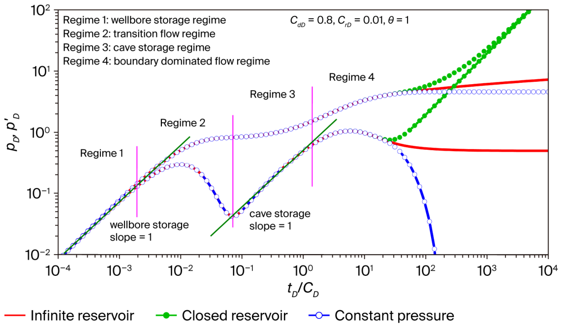
In this section, we plot the type curves of the wellbore pressure and its derivative under the three outer boundary conditions. The typical curves are plotted by using the values of the dimensionless pressure and pressure derivative versus dimensionless time. Type curve matching is a significant method in well tests, through which reservoir properties, such as the permeability, porosity, and cave volume, can be determined [31]. Figure 5 depicts the standard log–log curves of the pressure and pressure derivative under different external boundary conditions. We observed that there are four flow regimes, which are detailed below:

(1)

Flow regime 1 is the wellbore-storage regime. At very early time, the pressure disturbance has not propagated sufficiently into the surrounding formation, and the produced fluid is mainly supplied by fluid stored in the wellbore. Under a constant production-rate condition, the wellbore-storage relation produces an approximately linear pressure change with time. Consequently, both the pressure and pressure-derivative curves exhibit the characteristic unit-slope behavior on the log–log plot. As presented in Figure 5, the slopes of both the pressure and pressure derivative are equal to 1. This response is consistent with the classical interpretation of wellbore storage in pressure-transient analysis [27,29].

(2)

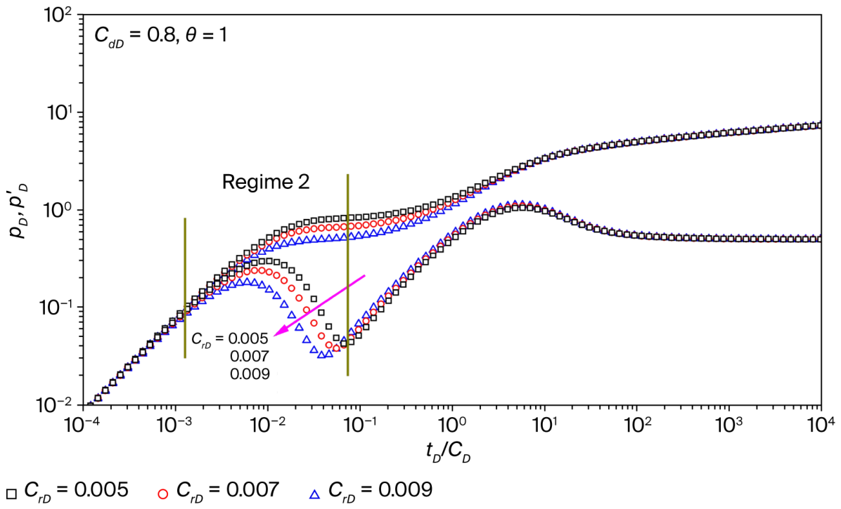
Flow regime 2 is the transition-flow regime. As the pressure disturbance propagates outward, the contributions from the surrounding formation and the large-scale cave become increasingly important. Within this regime, the wellbore-storage regime ends and gradually transits to regime 3, and an attached pressure drop is generated, which is similar to the skin effect. Therefore, as shown in Figure 5, the derivative curve rises first and descends later, and a concave appears. This concave illustrates the existence of the cave.

(3)

Flow regime 3 is the cave-storage regime. After the transition period, the contribution of cave storage becomes dominant. A substantial part of the produced fluid is supplied by the fluid stored in the large-scale cave, and the pressure response consequently approaches another storage-dominated behavior. Similar to regime 1, during this period, the oil is mainly produced by the cave storage effect. As shown in Figure 5, there is another straight line with slope one. The occurrence of a second storage-dominated regime distinguishes the cave-containing system from a conventional wellbore-storage response and demonstrates the significant role of cave storage in controlling the pressure transient.

(4)

Flow regime 4 is the boundary-dominated flow regime. At late time, the pressure disturbance reaches the outer boundary and the pressure response becomes governed by the imposed boundary condition. In this work, we investigate the curve behaviors under three kinds of external boundary conditions, which are all represented in Figure 5. For an infinite reservoir, the pressure-derivative approaches an approximately constant level because the pressure disturbance can continue to propagate outward without encountering a finite boundary. For a closed circular reservoir, no pressure support is supplied from outside the system, and the pressure derivative consequently rises with time. In contrast, for a finite reservoir maintained at constant pressure, the external pressure support reduces the pressure-decline rate and causes the pressure-derivative to decrease.

Overall, the four flow regimes provide a physical interpretation of the pressure response of a well connected to a large-scale cave. In particular, the transition and cave-storage regimes provide the principal dynamic information for identifying and characterizing the cave, whereas the late-time response reflects the external reservoir boundary. The behavior is also consistent with the broader understanding that fractured-vuggy carbonate reservoirs contain multiple storage and flow domains whose interactions can generate complex pressure-transient signatures [3,6,25].

5. Sensitivity Studies

In this section, the effects of each parameter on the pressure and pressure-derivative responses are investigated. In practice, well-tested data can be affected by many factors; therefore, it is essential to construct type curves under different conditions [32]. For convenience, we consider only the infinite reservoir, because the three external boundary conditions exhibit identical flow behavior during the first three regimes. The influence of the model parameters is primarily manifested during these regimes and is therefore essentially independent of the external boundary condition. The effects of the closed and constant-pressure boundaries emerge only in regime 4, where the boundary response dominates the pressure behavior. Thus, extending the parameter sensitivity analysis to the latter two boundary conditions would not introduce additional sensitivity characteristics, although the regime 4 responses differ among the three boundary conditions.

5.1. Effects of the Depth Coefficient C_dD

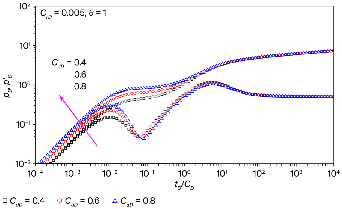
With all other parameters held constant, the pressure and pressure-derivative curves for different values of C_dD are plotted in Figure 6. According to the dimensionless definitions, C_dD is related to both cave depth and radius. However, as stated above, when C_rD is fixed, the C_dD mainly influences the cave depth. A higher C_dD therefore corresponds to a deeper cave.

For a cylindrical representation, the cave volume increases with the effective cave depth. Therefore, with $r_c$ fixed, increasing the effective cave depth increases the cave storage volume and consequently changes the characteristic time associated with the cave-storage response.

As shown in Figure 6, we can observe that the C_dD has an impact on the starting time of the wellbore-storage regime. The higher the C_dD, the earlier the wellbore-storage regime starts. As a ripple effect, the wellbore-storage regime ends earlier with the increase in the C_dD, which means the C_dD has no influence on the duration of the wellbore-storage regime. The characteristic slope of the storage-dominated segment is not substantially changed.

This behavior indicates that C_dD primarily affects the temporal position of the storage response rather than the detailed geometry of the pressure-derivative concavity. In physical terms, a change in cave depth modifies the available cave storage and therefore changes the time scale at which the cave begins to exert a noticeable influence on the wellbore pressure response. The limited influence of C_dD on the shape of the concave region further distinguishes the depth-related effect from the radius-related effect discussed below.

Thus, C_dD can be regarded primarily as a parameter controlling the effective vertical extent of the cave and the timing of the cave-related pressure response. Its effect on other flow regimes is minimal.

5.2. Effects of the Radius Coefficient C_rD

With all other parameters held constant, the pressure and pressure-derivative curves for different values of C_rD are plotted in Figure 7. According to the dimensionless definition, C_rD is related to cave radius. A higher C_rD corresponds to a larger cave. An increase in C_rD therefore corresponds to an increase in the lateral scale of the cave.

The physical significance of this relationship can be further understood from the geometric scaling of the cave. For a cylindrical cavity, $V_{cave}=\pi r_c^2{h}_2$, while the cave-formation interface through which radial fluid exchange occurs scales approximately with $r_c{h}_2$. Therefore, increasing $r_c$ simultaneously increases the storage capacity of the cave and the characteristic area available for fluid exchange between the surrounding formation and the cave. The effect of the radius is consequently more pronounced during the transition regime, when formation-cave interaction is active.

As shown in Figure 7, we can observe that the C_rD only influences regime 2, which means that the C_rD has an impact on the transition-flow regime. The higher the C_rD, the earlier the transition-flow regime appears and the derivative curve descends. Therefore, the width and depth of the concave shape are dominated by the C_rD, and the concave shape gradually becomes wider and deeper with the increasing C_rD.

This behavior indicates that the lateral scale of the cave strongly influences the duration and intensity of the transient interaction between the formation and the cave-storage domain. The dominant influence of C_rD on the concave response is physically consistent with previous analytical studies of multi-vug and large-cave carbonate reservoirs. Such studies have shown that vug/cave size and storage capacity strongly influence characteristic pressure-derivative response [25,33]. In particular, larger discrete storage spaces can produce more pronounced transient features because they provide greater volume for temporary fluid accumulation and redistribution.

Therefore, the width and depth of the concave feature provide useful information for constraining the effective radius of the large-scale cave. Compared with C_dD, C_rD has a much stronger influence on the detailed shape of the cave-related pressure response and is consequently an important parameter for cave-size estimation.

5.3. Effects of the Shape Coefficient θ

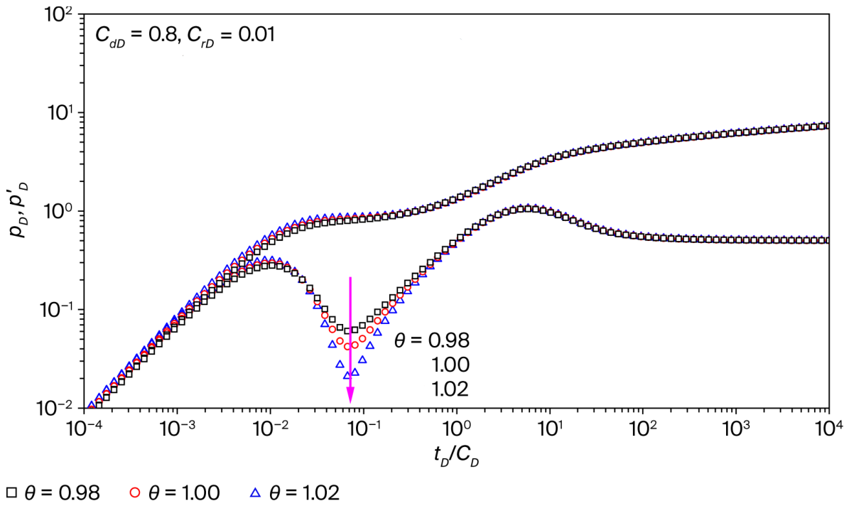
With all other parameters held constant, the pressure and pressure-derivative curves for different values of θ are plotted in Figure 8. As stated above, θ is introduced to approximately account for deviations of the actual cave geometry from the idealized cylindrical representation. This correction is motivated by geological observations from the Tarim Basin. In practice, a cave usually has an irregular shape. In the present model, θ = 1 corresponds to the cylindrical case, whereas deviations from unity represent an effective departure from that idealized geometry; θ < 1 represents a concave cylinder; and θ > 1 represents a convex cylinder. Accordingly, θ should not be interpreted as a complete three-dimensional descriptor of natural cave morphology. Instead, it represents a correction to the effective storage behavior of the cave.

As shown in Figure 8, we can observe that θ only influences the depth of the concave shape. A larger θ produces a deeper concave response, indicating that changes in effective cave geometry primarily modify the magnitude of the transient cave-related response. This behavior provides a physical interpretation of the role of θ: the geometry of the storage domain can alter the intensity of the pressure-transient signature even when its characteristic spatial and temporal scales remain approximately unchanged.

The importance of accounting for geometry is also supported by geological investigations of the Tahe Oilfield. Natural paleocaves can exhibit substantial morphological variability, and post-formational processes such as collapse, sedimentary filling, and hydrothermal modification can further alter their effective storage geometry. Thus, introducing a shape-correction parameter is preferable to assuming that all natural caves strictly conform to a cylindrical geometry.

5.4. Integrated Interpretation of the Cave-Related Parameters

The sensitivity results establish distinct roles for the three dimensionless parameters introduced in this study. The depth coefficient $C_{dD}$ primarily controls the effective vertical extent of the cave and therefore the timing of the storage-related response. The radius coefficient $C_{rD}$ controls the effective lateral scale of the cave and has the strongest influence on the width and depth of the concave pressure-derivative response. The shape coefficient θ provides an effective correction for deviations from the idealized cylindrical geometry and mainly modifies the magnitude of the concave response.

These different sensitivities provide the physical basis for the subsequent cave-volume interpretation. Specifically, $C_{rD}$ and $C_{dD}$ are first determined by matching the pressure and pressure-derivative-type curves and are then converted into the effective cave radius $r_c$ and depth $h_2$, respectively. The cave volume is subsequently calculated from these geometric parameters according to Equation (91) under the cylindrical-cave assumption. In contrast, the shape coefficient θ does not directly determine an independent geometric dimension in the present model; rather, it serves as an effective shape coefficient to account for deviations of the actual cave geometry from the idealized cylindrical shape and thereby modifies the pressure response associated with cave storage.

This interpretation is consistent with previous well-test studies showing that discrete vugs and caves can leave identifiable signatures in pressure-transient responses and that their storage characteristics can be evaluated through analytical type curve analysis [3,25,33]. At the same time, geological investigations indicate that natural fracture-cave systems are spatially heterogeneous and that cave geometry and filling can vary substantially [23,24]. Therefore, the parameters obtained from the present analytical model should be regarded as effective dynamic descriptors of the cave rather than exact three-dimensional geological measurements.

The above results also clarify the complementary roles of pressure and pressure-derivative in cave characterization. The pressure response reflects the overall storage and flow behavior of the system, whereas the pressure derivative more clearly distinguishes the transition caused by cave-formation interaction. The combined use of pressure and pressure-derivative-type curves therefore provides a more reliable basis for matching the model parameters and estimating the effective volume of a large-scale cave.

6. Field Example

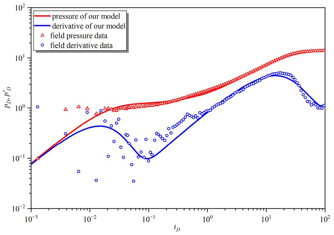
Large-scale caves are widespread in western China, where burial depths exceed 7000 m. In oil development, cave volume is an important parameter. Because no reliable well-test method has been established for calculating cave volume, geological techniques are commonly used, but they are more expensive and complex than well testing. To demonstrate the application of the proposed model to field data, we consider two example wells from the Shunbei Oilfield in Xinjiang, China. Both wells were completed using acidizing.

6.1. Example 1

The reservoir properties of the first well are listed in

Table 2. Reservoir properties of Example Well 1.

Parameters	Values	Units
Formation thickness	10.0000	m
Wellbore radius	0.0746	m
Initial pressure pi	83.5800	MPa
Porosity	0.10	fraction
Oil viscosity	0.0003	Pa·s
Oil formation volume factor	1.1000	fraction
Oil density	600.0000	kg/m3
Fluid compressibility	0.0021	MPa−1
Middle depth	7557.6600	m

. During the 7-9-11-12.5-11-9-7 mm choke-size test sequence, the well produced 46.75 × 10⁴ m³/d of gas, 93.84 m³/d of total liquid, and 89.15 m³/d of oil, with a water cut of 5% and a gas-oil ratio of 5244 m³/m³. The production rate per unit pressure drop was 85.96 × 10⁴ m³/MPa, and the wellhead pressure declined at a rate of 0.82 MPa/d.

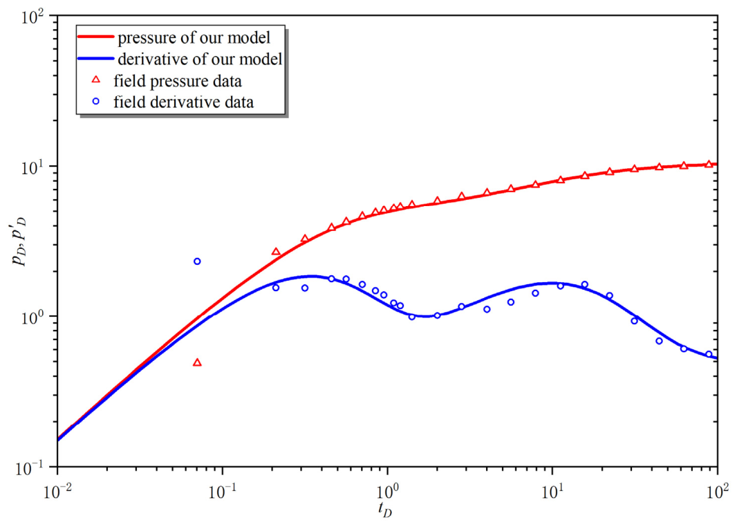
Figure 9 shows the type curve matching of the pressure and pressure derivative, with good agreement between the theoretical and field data. The interpretation results are listed in

Table 3. Interpretation results for Example Well 1.

Parameters	Values	Units
Permeability	77.4637	mD
Depth coefficient CdD	0.8057	fraction
Radius coefficient CrD	0.0145	fraction
Cave volume	18,235.1256	m3
Skin factor	4.1421	fraction
Wellbore storage constant C	1.7779	m3/MPa
Cave storage constant Ccave	37.8297	m3/MPa

. According to these results, the estimated cave volume is 18,235.1256 m³, which is consistent with the geological estimate of 15,000–20,000 m³ for the cave volume.

6.2. Example 2

The reservoir properties of the second well are listed in

Table 4. Reservoir properties of Example Well 2.

Parameters	Values	Units
Formation thickness	10.0000	m
Wellbore radius	0.0826	m
Average pressure	57.8794	MPa
Porosity	0.10	fraction
Oil viscosity	0.0003	Pa·s
Oil formation volume factor	1.1000	fraction
Oil density	600.0000	kg/m3
Fluid compressibility	0.0021	MPa−1
Middle depth	8109.9500	m

. During the 9-12-14-9 mm choke-size test sequence, the well produced oil at a rate of 214.60 m³/d, with a water cut of 1% and a gas production rate of 34.09 × 10⁴ m³/d. The gas-oil ratio was 1589 m³/m³. All production parameters remained relatively stable throughout the tests.

Figure 10 shows the type curve matching of the pressure and pressure derivative, with good agreement between the theoretical and field data. The interpretation results are listed in

Table 5. Interpretation results for Example Well 2.

Parameters	Values	Units
Permeability	587.6	mD
Depth coefficient CdD	0.29275	fraction
Radius coefficient CrD	0.0132	fraction
Cave volume	32,280.99	m3
Cave storage constant Ccave	67.7901	m3/MPa

. According to these results, the estimated cave volume is 32,280.99 m³, which is consistent with the geological estimate of 30,000–50,000 m³ for the cave volume.

7. Conclusions

In this work, we analytically investigate the pressure and pressure-derivative responses of the proposed well-test model. Based on the results, the following conclusions can be drawn:

(1)

A novel well-test model is proposed for estimating the volume of large-scale caves in carbonate reservoirs.

(2)

A mathematical model is established, and the analytical solution is derived using the Laplace transformation. Using numerical inversion, standard log–log curves of the pressure and pressure derivative are plotted. We observe four distinct flow regimes and a pronounced concave feature.

(3)

Sensitivity studies demonstrate that the curve behavior is influenced by the C_dD, C_rD, and θ. The C_dD mainly affects the onset of the wellbore-storage regime; C_rD influences the width and depth of the concave section; and θ controls the depth of the concave feature.

(4)

Two field cases are presented to validate the applicability of the proposed model. The estimated cave volumes agree well with the ranges obtained from independent geological characterization, demonstrating that the proposed model provides an effective approach to cave-volume determination.

References

1. Xing, C.; Yin, H.; Yuan, H.; Fu, J.; Xu, G. Pressure-transient Analysis for Fracture-Cavity Carbonate Reservoirs with Large-Scale Fractures–Caves in Series Connection. J. Energy Resour. Technol. 2021, 144, 052901. [Google Scholar] [CrossRef] [Scilit]
2. Wang, M.; Fan, Z.; Dong, X.; Song, H.; Zhao, W.; Xu, G. Analysis of Flow Behavior for Acid Fracturing Wells in Fractured-Vuggy Carbonate Reservoirs. Math. Probl. Eng. 2018, 2018, 6431910. [Google Scholar] [CrossRef] [Scilit]
3. Du, X.; Lu, Z.W.; Li, D.M.; Xu, Y.D.; Li, P.C.; Lu, D.T. A novel analytical well test model for fractured vuggy carbonate reservoirs considering the coupling between oil flow and wave propagation. J. Pet. Sci. Eng. 2019, 173, 447–461. [Google Scholar] [CrossRef] [Scilit]
4. Wei, C.; Liu, Y.; Deng, Y.; Cheng, S.; Hassanzadeh, H. Analytical well-test model for hydraulicly fractured wells with multiwell interference in double porosity gas reservoirs. J. Nat. Gas Sci. Eng. 2022, 103, 104624. [Google Scholar] [CrossRef] [Scilit]
5. Chen, D.; Sun, Z. A Semi-Analytical Model for Gas–Water Two-Phase Productivity Prediction of Carbonate Gas Reservoirs. Processes 2023, 11, 591. [Google Scholar] [CrossRef] [Scilit]
6. Liang, Q.; Chen, R.; Yan, W. Research progress and challenges of flow mechanisms and well-testing models in carbonate reservoirs. Front. Energy Res. 2023, 11, 1274448. [Google Scholar] [CrossRef] [Scilit]
7. Du, X.; Li, Q.; Li, P.; Xian, Y.; Zheng, Y.; Lu, D. A novel pressure and rate transient analysis model for fracture-caved carbonate reservoirs. J. Pet. Sci. Eng. 2022, 208, 109609. [Google Scholar] [CrossRef] [Scilit]
8. Braitenberg, C.; Sampietro, D.; Pivetta, T.; Zuliani, D.; Barbagallo, A.; Fabris, P.; Rossi, L.; Fabbri, J.; Mansi, A.H. Gravity for Detecting Caves: Airborne and Terrestrial Simulations Based on a Comprehensive Karstic Cave Benchmark. Pure Appl. Geophys. 2016, 173, 1243–1264. [Google Scholar] [CrossRef] [Scilit]
9. Cardarelli, E.; Cercato, M.; Cerreto, A.; Di Filippo, G. Electrical resistivity and seismic refraction tomography to detect buried cavities. Geophys. Prospect. 2010, 58, 685–695. [Google Scholar] [CrossRef] [Scilit]
10. Van Hout, G.; Taylor, K.; Van As, A. A novel methodology for verifying height of draw in a cave mine through drawpoint sampling and drawpoint geological observations. In Proceedings of the 26th World Mining Congress, Brisbane, Australia, 26–29 June 2023. [Google Scholar]
11. Fabbri, S.; Sauro, F.; Santagata, T.; Rossi, G.; De Waele, J. High-resolution 3-D mapping using terrestrial laser scanning as a tool for geomorphological and speleogenetical studies in caves: An example from the Lessini mountains (North Italy). Geomorphology 2017, 280, 16–29. [Google Scholar] [CrossRef] [Scilit]
12. Cazes, G.; Vernant, P.; Baleux, F.; Giuliani, C.; Jouves, J.; Brugal, J.-P. Full size cave 3D modelling using close range photogrammetry and comparison with laser scanning. Appl. Geomat. 2025, 17, 733–747. [Google Scholar] [CrossRef] [Scilit]
13. Zhang, C.; Chen, J.; Li, P.; Han, S.; Xu, J. Integrated high-precision real scene 3D modeling of karst cave landscape based on laser scanning and photogrammetry. Sci. Rep. 2024, 14, 20485, Correction in Sci. Rep. 2025, 15, 4345. https://doi.org/10.1038/s41598-025-88453-y. [Google Scholar] [CrossRef] [Scilit] [PubMed]
14. Chen, P.; Wang, X.; Liu, H.; Huang, Y.; Chen, S.; Zhang, H. A pressure-transient model for a fractured-vuggy carbonate reservoir with large-scale cave. Geosystem Eng. 2016, 19, 69–76. [Google Scholar] [CrossRef] [Scilit]
15. Wan, Y.-Z.; Liu, Y.-W.; Chen, F.-F.; Wu, N.-Y.; Hu, G.-W. Numerical well test model for caved carbonate reservoirs and its application in Tarim Basin, China. J. Pet. Sci. Eng. 2018, 161, 611–624. [Google Scholar] [CrossRef] [Scilit]
16. Li, Q.; Du, X.; Tang, Q.; Xu, Y.; Li, P.; Lu, D. A novel well test model for fractured vuggy carbonate reservoirs with the vertical bead-on-a-string structure. J. Pet. Sci. Eng. 2021, 196, 107938. [Google Scholar] [CrossRef] [Scilit]
17. Yue, P.; Xie, Z.; Liu, H.; Chen, X.; Guo, Z. Application of water injection curves for the dynamic analysis of fractured-vuggy carbonate reservoirs. J. Pet. Sci. Eng. 2018, 169, 220–229. [Google Scholar] [CrossRef] [Scilit]
18. Xu, X.; Chen, Q.; Chu, C.; Li, G.; Liu, C.; Shi, Z. Tectonic evolution and paleokarstification of carbonate rocks in the Paleozoic Tarim Basin. Carbonates Evaporites 2017, 32, 487–496. [Google Scholar] [CrossRef] [Scilit] [PubMed]
19. Camacho-Velazquez, R.; Vasquez-Cruz, M.; Castrejon-Aivar, R.; Arana-Ortiz, V. Pressure-transient and decline-curve behavior in naturally fractured vuggy carbonate reservoirs. SPE Reserv. Eval. Eng. 2005, 8, 95–112. [Google Scholar] [CrossRef] [Scilit]
20. Yao, J.; Huang, Z.-Q. Fractured Vuggy Carbonate Reservoir Simulation; Springer: Berlin/Heidelberg, Germany, 2017. [Google Scholar]
21. Kang, Z.; Di, Y.; Cui, S. Numerical Simulation Technology and Application of Fractured-Vuggy Carbonate Reservoirs, 1st ed.; China University of Petroleum Press: Qingdao, China, 2017. [Google Scholar]
22. Mousavi, M.; Prodanovic, M.; Jacobi, D. New classification of carbonate rocks for process-based pore-scale modeling. SPE J. 2013, 18, 243–263. [Google Scholar] [CrossRef] [Scilit]
23. Jin, Q.; Tian, F.; Lu, X.; Kang, X. Characteristics of collapse breccias filling in caves of runoff zone in the Ordovician karst in Tahe Oilfield, Tarim Basin. Oil Gas Geol. 2015, 36, 729–735. [Google Scholar] [CrossRef]
24. Zhang, H.; Cai, Z.; Hao, F.; Hu, W.; Lu, X.; Wang, Y. Hypogenic origin of paleocaves in the Ordovician carbonates of the southern Tahe oilfield, Tarim basin, northwest China. Geoenergy Sci. Eng. 2023, 225, 211669. [Google Scholar] [CrossRef] [Scilit]
25. Du, X.; Li, Q.; Lu, Z.; Li, P.; Xian, Y.; Xu, Y.; Li, D.; Lu, D. Pressure-transient analysis for multi-vug composite fractured vuggy carbonate reservoirs. J. Pet. Sci. Eng. 2020, 193, 107389. [Google Scholar] [CrossRef] [Scilit]
26. Du, X.; Zhang, Y.; Zhou, C.; Su, Y.; Li, Q.; Li, P.; Lu, Z.; Xian, Y.; Lu, D. A novel method for determining the binomial deliverability equation of fractured caved carbonate reservoirs. J. Pet. Sci. Eng. 2022, 208, 109496. [Google Scholar] [CrossRef] [Scilit]
27. Van Everdingen, A.F.; Hurst, W. The Application of the Laplace Transformation to Flow Problems in Reservoirs. J. Pet. Technol. 1949, 1, 305–324. [Google Scholar] [CrossRef] [Scilit]
28. Li, Q.Y.; Li, P.C.; Pang, W.; Li, D.L.; Liang, H.B.; Lu, D.T. A new method for production data analysis in shale gas reservoirs. J. Nat. Gas. Sci. Eng. 2018, 56, 368–383. [Google Scholar] [CrossRef] [Scilit]
29. Stehfest, H. Algorithm 368: Numerical inversion of Laplace transforms [D5]. Commun. ACM 1970, 13, 47–49. [Google Scholar] [CrossRef] [Scilit]
30. He, S.; Chen, B.; Yuan, F.; Wang, X.; Wang, T. Dynamic Reserve Calculation Method of Fractured-Vuggy Reservoir Based on Modified Comprehensive Compression Coefficient. Processes 2024, 12, 640. [Google Scholar] [CrossRef] [Scilit]
31. Li, Q.Y.; Li, P.C.; Pang, W.; Huang, J.P.; Liang, H.B.; Lu, D.T. A method for production data analysis considering significant discontinuities in unconventional reservoirs. J. Geophys. Eng. 2018, 15, 1835–1842. [Google Scholar] [CrossRef] [Scilit]
32. Zhao, Y.L.; Tang, X.C.; Zhang, L.H.; Tang, H.M.; Tao, Z.W. Numerical solution of fractured horizontal wells in shale gas reservoirs considering multiple transport mechanisms. J. Geophys. Eng. 2018, 15, 739–750. [Google Scholar] [CrossRef] [Scilit]
33. Gao, B.; Huang, Z.-Q.; Yao, J.; Lv, X.-R.; Wu, Y.-S. Pressure-transient analysis of a well penetrating a filled cavity in naturally fractured carbonate reservoirs. J. Pet. Sci. Eng. 2016, 145, 392–403. [Google Scholar] [CrossRef] [Scilit]
Figure 1. Workflow of the proposed analytical method for estimating large-scale cave volume.
Processes 14 02966 g001
Figure 2. Schematic of the physical model.
Processes 14 02966 g002
Figure 3. Schematic of energy conservation at the cave-wellbore interface.
Processes 14 02966 g003
Figure 4. Infinitesimal control volume in the wellbore.
Processes 14 02966 g004
Figure 5. Pressure and pressure-derivative-type curves under different outer boundary conditions.
Processes 14 02966 g005
Figure 6. Sensitivity of pressure and pressure derivative to CdD.
Processes 14 02966 g006
Figure 7. Sensitivity of pressure and pressure derivative to CrD.
Processes 14 02966 g007
Figure 8. Sensitivity of pressure and pressure derivative to θ.
Processes 14 02966 g008
Figure 9. Type curve matching of pressure and pressure-derivative for Example Well 1.
Processes 14 02966 g009
Figure 10. Type curve matching of pressure and pressure-derivative for Example Well 2.
Processes 14 02966 g010