The Hybrid DBSCAN-Transformer Framework for High-Precision Phase Fraction Measurement in Low-Energy Gamma Flowmeter

Abstract

Multiphase flow metering is widely employed in the oil and gas industry, particularly for measuring gas-liquid-solid multiphase flow at drilling outlets. Low-energy gamma flowmeters offer relatively high metering accuracy, with phase fraction errors for gas, liquid, and solid typically within ±10%. However, in practical applications, fluid viscosity often causes substances to adhere to the photon detector, leading to measurement deviations that can reach 18% or more. To overcome this limitation, this paper proposes a hybrid Density-Based Spatial Clustering of Applications with Noise (DBSCAN)-Transformer regression framework, referred to as D-Transformer. DBSCAN removes isolated abnormal detector responses before overlapping time-series windows are generated, while the Transformer captures temporal dependencies among operating variables, raw phase-fraction readings, and multi-energy photon counts. Under experiment-wise five-fold evaluation, D-Transformer obtains $R^2$ values of 0.982, 0.985, and 0.981 and RMSE values of 0.0134, 0.0122, and 0.0138 for the gas, liquid, and solid phase fractions, respectively. Component ablations and baseline comparisons show that the complete framework outperforms the no-ResNet, no-DBSCAN, CNN-GRU-Attention, CNN-LSTM, ridge-regression, and uncorrected-flowmeter alternatives.

1. Introduction

Multiphase flow is widely present in industries such as petroleum, chemical, metallurgical, and power generation [1,2]. In oil and gas drilling processing, the wellhead return fluid is mainly composed of drilling fluid, downhole rock debris, natural gas, and groundwater. The return fluid is thus a multiphase mixture consisting of a gas-liquid-solid flow. At the wellhead position of drilling operations, accurate metering of gas-liquid solid phase substances in the return fluid can help engineers understand the geological conditions of drilling, which can prevent drilling safety accidents.

In traditional multiphase flow metering methods, there are mainly radioactive ray metering method, nuclear magnetic resonance metering method, Coriolis force metering method, and capacitance volume imaging metering method. In radioactive ray metering method, Song has developed a compact X-ray densitometry system consisting of a 50 kV, 1mA X-ray tube and several linear detector arrays, which used to measure the density of two-phase flow [3]. Basahel has utilized an artificial neural network (ANN) and various feature extractions to enhance the precision of X-ray radiation-based two-phase flowmeters [4]. Taylan proposed the Radial Basis Function Neural Networks to determine the type of flow regimes and predict the volume fractions of gas-oil-water three-phase flows [5].

In nuclear magnetic resonance metering method, Bilgic developed a multiphase flow meter based on magnetic resonance, which is capable of producing a spatial distribution image for oil-water multiphase flow [6]. Meribout has presented an optimal coil and the magnets arrays design of the multiphase flow meter, which is based on nuclear magnetic resonance and magnetic resonance imaging [7]. Meribout also proposed a novel Halbach array-based nuclear magnetic resonance device for multiphase flow metering, which used a 3-D finite-element method (FEM)-based software combined with particle swarm optimization algorithm [8].

In Coriolis force metering method, Meribout presented a new Coriolis-based two-phase flowmeter (TPFM) that used an upstream inline flow conditioner which separated liquid from gas [9]. Fadaei has used a soft sensor to predict the gas volume fraction within gas-liquid flow, and studied the variation of Coriolis meter factor with gas volume fraction and Reynolds number [10]. Chowdhury established three different data-driven models based on support vector machine, artificial neural network, and Gaussian process regression, which are incorporated into Coriolis flowmeters for mass flowrate measurement of two-phase (sand-water) slurry [11].

In capacitance volume imaging metering method, Zeeshan has enhanced resolution of electrical capacitive sensors for multiphase flow measurement by fine-stepped electronic scanning of synthetic electrodes [12]. Sun presented a method for real-time 3-D imaging and velocity measurement of two-phase flows using a twin-plane electrical capacitance tomography sensor with 24 electrodes [13]. Mota presented a water volume fraction estimation method based on electrical capacitance tomography, which is applied to assist flow pattern identification routines as well as to estimate two-phase flow rates [14].

These multiphase flow metering methods have achieved certain results, but there are also some drawbacks. Radioactive ray or nuclear magnetic resonance flowmeters pose a nuclear radiation safety threat to the environment and people. The Coriolis flowmeter’s accuracy is primarily limited to single-phase flows or specific oil-water mixtures, and it is generally unsuitable for default gas-liquid two-phase flows without advanced conditioning. The capacitance volume imaging flowmeter is a volumetric metering device that cannot measure the mass flow rate for multiphase flow.

The low-energy gamma flowmeter is a new type of multiphase flowmeter, which was jointly developed by Southwest Petroleum University and Chengdu Yangpai Technology Co., Ltd. [15]. In low-energy gamma flowmeter, the core technology is to use the absorption degree of light quantum by gas, oil or water (liquid), and solid phase substances to achieve phase fraction measurement. Under stable multiphase flow conditions, the low-energy gamma flowmeter measurement error of phase fractions for oil, gas, water, and solid substances is within ±10%. In order to correct this phase-fraction measurement error, we use deep learning to capture temporal characteristics and regress the synchronized reference phase fractions. This software-based correction avoids changing the mechanical structure of the low-energy gamma flowmeter and is therefore economical and efficient.

Representative international studies have applied X-ray densitometry and neural networks to two-phase flow measurement [3,4], radial-basis-function networks to gas-oil-water fraction prediction [5], and soft sensors or conventional machine-learning models to conditioned Coriolis and slurry measurements [10,11]. These studies establish the value of data-driven compensation, but most focus on two-phase systems, static or pointwise features, or laboratory and conditioned-meter configurations. The domestic low-energy gamma flowmeter development in Ref. [15] established the multi-energy photon-measurement hardware, whereas the present work focuses on software correction under detector adhesion and drilling-return disturbances. The core innovations of this study are therefore: (1) scenario-specific DBSCAN denoising before window construction, preventing one isolated detector disturbance from contaminating multiple overlapping samples; (2) a Transformer regression model with learnable positional encoding for dynamic gas-liquid-solid measurements; (3) a ResNet-MLP compositional output head that enforces non-negative fractions summing to unity; and (4) evaluation using both a controlled loop and an operating-well field case with independent reference instrumentation.

This paper mainly consists of the following five parts, with Section 1 is the introduction. Section 2 describes the background of the multiphase flow metering with low-energy gamma flowmeter. Section 3 uses the deep learning to improve the phase fractions accuracy of low-energy gamma flowmeter. Section 4 is the part of low-energy gamma flowmeter experiment. Finally, Section 5 is the conclusion part.

2. Background of the Multiphase Flow Metering with Low-Energy Gamma Flowmeter

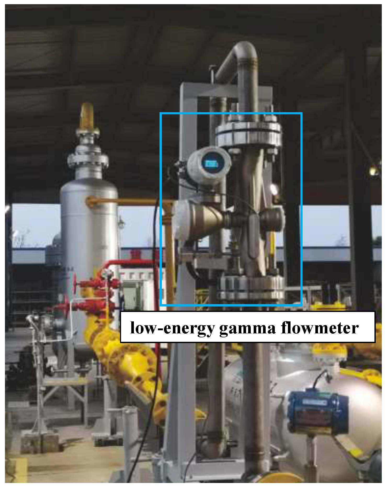
Figure 1 is a low-energy gamma flowmeter, which uses a venturi tube to measure the total mass flow rate Q of the multiphase flow, and then, the light quantum absorption technology is used to measure the phase fraction of multiphase flow, including the oil mass fraction (OMF), gas mass fraction (GMF), water mass fraction (WMF), and solid mass fraction (SMF). Multiplying the total flow rate Q by the phase fractions (GMF, OMF, WMF, SMF) yields the mass flow rates of gas, oil, water, and solids.

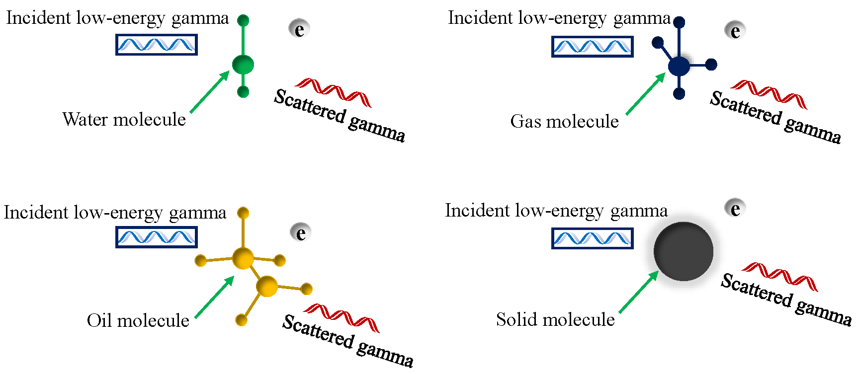
The core of low-energy gamma flowmeter is photon absorption technology. In photon absorption technology, the photon sensor radiates a set of photons with multiple energy levels (31 KeV, 81 KeV, 160 KeV, 356 KeV). Photons have a strong ability to penetrate multiphase flow media, and their energy intensity is weakened due to the absorption effect of the multiphase flow media. Figure 2 shows the principle of photon absorption for oil, gas, water, and solid substances.

The photon scintillation detector measures the energy intensity of each photon group transmitted through the multiphase flow. The linear masses $q_{g,i}$, $q_{o,i}$, $q_{w,i}$, and $q_{s,i}$ ($i\in \{31,81,160,356\}$) of gas, oil, water, and solid, respectively, can then be calculated from the measured photon energy intensities. Linear mass refers to the mass of a phase intersected by the photon beam. Further calculations yield the mass fractions of gas, oil, water, and solids.

$$\left\{\begin{array}{c}\mathrm{GMF}={\displaystyle \frac{q_{g,i}}{q_{g,i}+q_{o,i}+q_{w,i}+q_{s,i}}}\hfill \\ \mathrm{OMF}={\displaystyle \frac{q_{o,i}}{q_{g,i}+q_{o,i}+q_{w,i}+q_{s,i}}}\hfill \\ \mathrm{WMF}={\displaystyle \frac{q_{w,i}}{q_{g,i}+q_{o,i}+q_{w,i}+q_{s,i}}}\hfill \\ \mathrm{SMF}={\displaystyle \frac{q_{s,i}}{q_{g,i}+q_{o,i}+q_{w,i}+q_{s,i}}}\hfill \end{array}\right.$$

(1)

Thus, the mass flow rates of gas, oil, water, and solids can be calculated as follows.

$$\left\{\begin{array}{c}{Q}_g=Q·\mathrm{GMF},Q_o=Q·\mathrm{OMF},\hfill \\ Q_w=Q·\mathrm{WMF},Q_s=Q·\mathrm{SMF}\hfill \end{array}\right.$$

(2)

In Equation (2), Q is the total mass flow rate of the multiphase flow, while $Q_g$, $Q_o$, $Q_w$, and $Q_s$ are the gas-, oil-, water-, and solid-phase mass flow rates, respectively. Thus, accurate phase-fraction measurement is the core requirement for gas-liquid-solid multiphase metering with the low-energy gamma flowmeter.

However, in actual multiphase flow metering, due to the viscosity of multiphase flow, multiphase flow substances are highly likely to adhere to the light quantum detector, resulting in measurement deviations of the light quantum detector for the phase fractions. The measurement deviation can even reach ±18% or more. Thus, to achieve the optimal measurement accuracy, we utilize the proposed D-Transformer algorithm to correct the measured phase fractions data.

3. Deep Learning Improves the Phase Fractions of Low-Energy Gamma Flowmeter

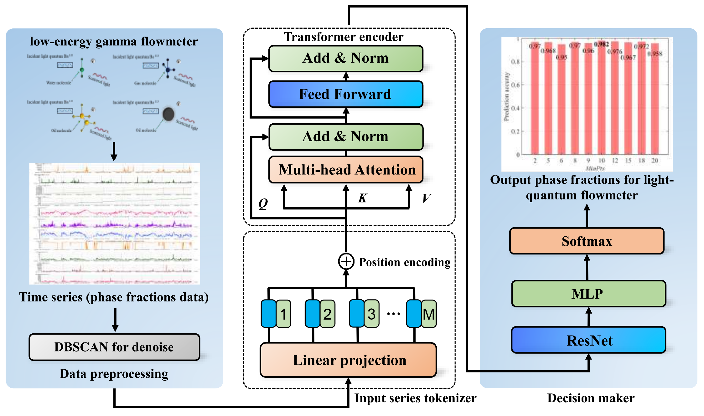
In this paper, we use an improved transformer deep algorithm to correct the phase fractions accuracy of the low-energy gamma flowmeter. The overall architecture of the improved transformer algorithm for phase fractions correction is shown in Figure 3. The first step is data preprocessing, which primarily including DBSCAN denoising for the low-energy gamma flowmeter phase fractions data. Then, the phase fractions correction is composed of an input series tokenizer, a transformer encoder and a decision maker.

The advantages of deep learning algorithms are as follows: 1. Considering the potential safety factor, although the half cycle of the light-quantum flowmeter is within the exemption level range, there is still trace radiation, and the software algorithm correction technique can avoid the light-quantum flowmeter structure optimization. 2. By using deep learning algorithm to improve the phase fractions accuracy of flowmeter, there is no need to optimize the hardware structure of existing low-energy gamma flowmeter, resulting in lower economic costs. 3. The deep learning algorithm can be continuously optimized and adjusted in reverse based on measurement errors. The algorithm can be flexibly used to correct phase fractions accuracy until the optimal accuracy is achieved.

3.1. The Transformer Regression Model Optimized by DBSCAN

Pseudo or singular values in the low-energy gamma flowmeter measurement data are typical noises, which resulting in a threat to the calibration process of the flowmeter phase fractions accuracy. The DBSCAN cluster has excellent recognition ability for noise points in dataset [16], therefore, we use the DBSCAN to remove noise points in the light-quantum measurement dataset. Before introducing the DBSCAN clustering process, it is necessary to clarify the following basic parameter definitions of DBSCAN.

The DBSCAN stage is specifically adapted to the noise mechanism of the low-energy gamma flowmeter. Adhesion of viscous drilling fluid to the detector window and short-term detector disturbances can generate isolated abnormal photon counts and phase-fraction readings. DBSCAN is applied to the normalized multi-parameter measurement vectors, including operating variables, measured phase fractions, and photon counts at 31, 81, 160, and 356 keV. Points identified as density-isolated noise are removed before the time-series windows are constructed. This procedure prevents isolated detector responses from propagating through multiple overlapping windows while preserving the chronological order of the retained measurements. In the present study, the neighborhood radius and density threshold were set to $\mathrm{Eps}=0.6$ and $\mathrm{MinPts}=10$, respectively.

Neighborhood (Eps): This is the circular region of radius $\epsilon$ centered on each data point p in dataset D. Any data point q that falls within this region belongs to the Eps neighborhood of p.

Density threshold (MinPts): The number of data points that fall within the Eps neighborhood of a point p defines its local density; MinPts is the minimum density threshold used to determine whether p is a core point.

Core point: If the density of a data point p is greater than or equal to MinPts, then p is a core point.

Edge point: When the density of a data point p is lower than MinPts but p lies within the Eps neighborhood of a core point, it is an edge point.

Noise point: If the density of a data point p is lower than MinPts and p does not lie within the Eps neighborhood of any core point, it is a noise point.

Direct density reachable: For the core point x and any data point y, if the data point x is located within the neighborhood Eps of the core point x, then point x and y are said to have direct density reachable.

Density achievable: For data point $x_1,x_2,\dots ,x_{\mathrm{n}}$ in the dataset D, if $\mathrm{n}\ge 2$ and satisfies the density reachable directly from $x_{\mathrm{i}}$ to $x_{\mathrm{i}+1}$, then data points $x_1,x_2,\dots ,x_{\mathrm{n}}$ are called density reachable.

Density connected: If there are data points $p_{\mathrm{x}}$ to $p_{\mathrm{y}}$ and $p_z$ in the dataset D that are density reachable, then data points $p_{\mathrm{y}}$ and $p_z$ are said to be density connected.

In practical DBSCAN application, the neighborhood Eps and density threshold MinPts are first specified to identify core points. A core point p is selected as the starting point, and directly density-reachable core points are connected. Edge points are then assigned to the nearest core points until all density-connected points form the required clusters, leaving isolated observations as noise. In the low-energy gamma flowmeter measurements, DBSCAN identifies and removes such noise points from the phase-fraction data before model calibration.

3.2. Improved Transformer Algorithm

In 2017, Google proposed the transformer, which is a deep learning model based on attention mechanism [17]. Transformer is mainly used for processing sequence to sequence tasks. Considering that low-energy gamma flowmeter data is essentially a time series of multiphase flow parameters, we chose to conduct research on the transformer calibration algorithm for the metering accuracy of low-energy gamma flowmeter. In this study, the input sequence tokenizer, Transformer encoder, and ResNet-MLP decision module form a multi-output regression model. The model jointly embeds the 11 metering variables, captures their temporal dependence through positional encoding and multi-head attention, and predicts the continuous gas, liquid, and solid phase fractions. The final Softmax operation imposes non-negativity and a unit-sum constraint on the three predicted fractions.

3.2.1. Input Series Tokenizer

In transformer architecture, the time-series tokenizer is a fundamental unit, used to segment input time series data into discrete tokens. The value 3385 denotes the number of chronological records in one representative continuous experimental sequence, rather than the size of the complete dataset. The complete dataset contains 20,000 records collected from multiple repeated experiments and operating stages. For each experimental run, the records are first ordered by acquisition time and are then converted into samples using a sliding window of $W=20$ consecutive time points and a step size of $S=1$. With $L=11$ input variables, the ith model input is $x_i\in {\mathbb{R}}^{W\times L}={\mathbb{R}}^{20\times 11}$, and the corresponding target $y_i\in {\mathbb{R}}^3$ is the reference gas, liquid, and solid phase fractions at the final time point of that window. For a run containing M valid chronological records, the number of windows is

$$N_{\mathrm{win}}=⌊{\displaystyle \frac{M-W}{S}}⌋+1.$$

Windows are constructed independently within each experimental run and are not allowed to cross experiment, training, validation, or test boundaries. A learnable linear projection maps each window to the embedding $z_i\in {\mathbb{R}}^{W\times d_{\mathrm{model}}}$, where $d_{\mathrm{model}}$ is the embedding dimension. The embedding process can be defined as follows:

$$z=x{W}_e+b_e,$$

(3)

where $W_e\in {\mathbb{R}}^{11\times d_{\mathrm{model}}}$ and $b_e\in {\mathbb{R}}^{d_{\mathrm{model}}}$ are the learnable projection parameters.

A learnable positional-encoding matrix $E_{\mathrm{pos}}\in {\mathbb{R}}^{W\times d_{\mathrm{model}}}$ is then added to the projected sequence. In the implemented configuration, $W=20$ and $d_{\mathrm{model}}=32$, so $E_{\mathrm{pos}}\in {\mathbb{R}}^{20\times 32}$. Each row of $E_{\mathrm{pos}}$ represents one relative time position in the window. The matrix is randomly initialized and optimized jointly with the remaining network parameters through back-propagation; it is not computed using a fixed sinusoidal rule. For sample i and position t, the encoder input is

$$X_{i,t}=z_{i,t}+E_{\mathrm{pos}}[t,:],t=1,\dots ,W.$$

(4)

This implementation allows the model to learn the relative temporal structure specific to the 20-point low-energy gamma measurement window.

3.2.2. Multi-Head Attention

For each element in the sequence, the attention mechanism calculates its similarity with other elements and normalizes these similarities into attention weights. Then, by weighting and summing each element with its corresponding attention weight, the self-attention mechanism output can be obtained. In transformer encoder, attention mechanisms are widely used, including scaled dot-product attention (SDPA) and multi-head attention (MHA).

In SDPA, its inputs include a query Q vector and a key K vector with dimensions $d_k$, as well as a value V vector with dimensions $d_v$. Perform dot product on all Q vectors and K vectors, divide by $\sqrt{d_k}$, and then use softmax function to obtain the weights of attention.

$$Attention(Q,K,V)=softmax\left(Q{K}^T/\sqrt{d_k}\right)V$$

(5)

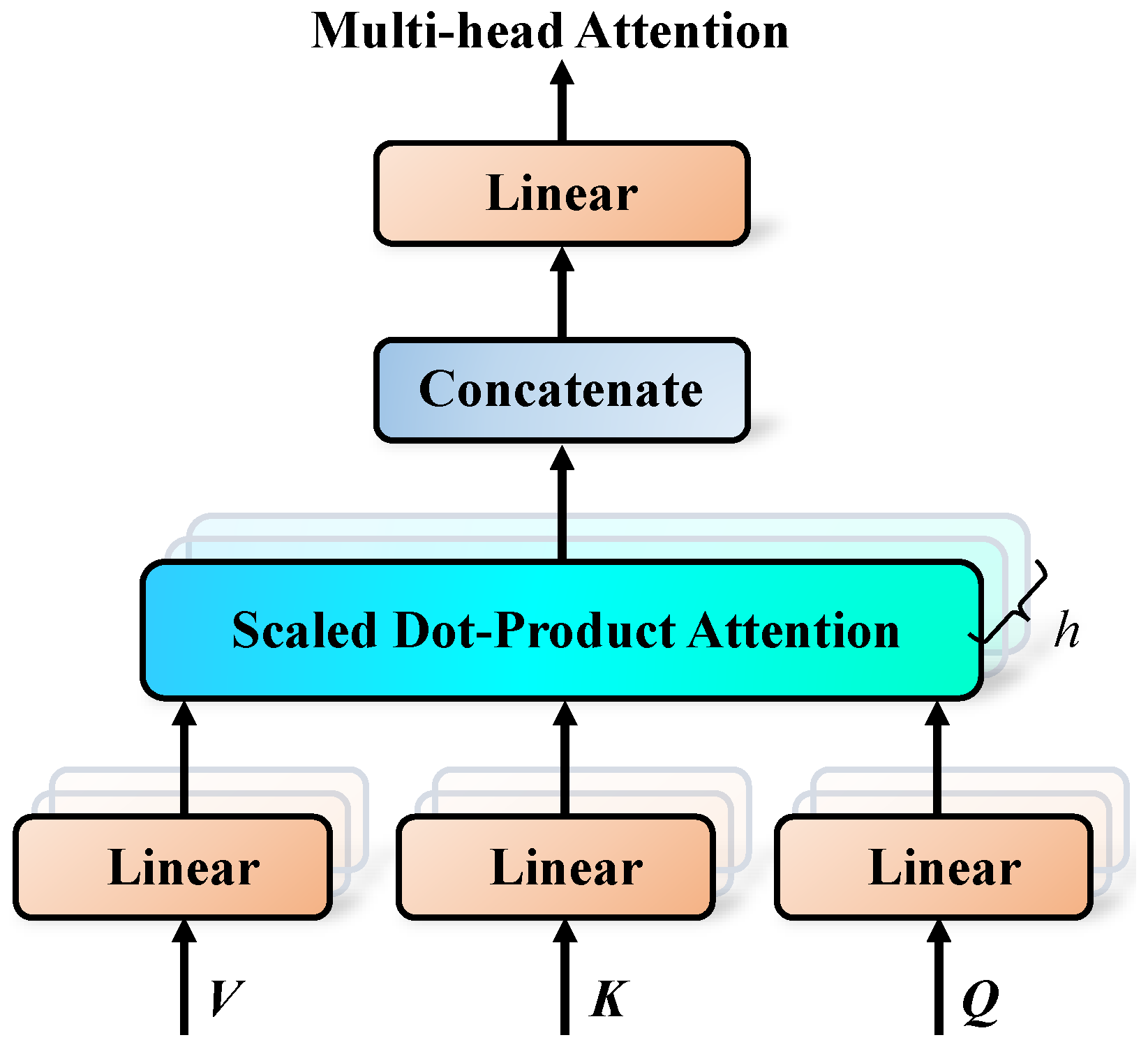
As shown in Figure 4, MHA is motivated by the opportunity to explore multiple representation subspaces, as each attention head obtains a different projection of the representation, and concatenates the resulting representations together to improve the model to capture different features and representations.

$$\left\{\begin{array}{c}\mathrm{head}=Attention\left(Q{W}^Q,K{W}^K,V{W}^V\right)\hfill \\ \mathrm{MultiHead}(Q,K,V)={\mathrm{Concat}}^{\left({\mathrm{head}}_1,\dots ,{\mathrm{head}}_n\right)W^o}\hfill \end{array}\right.$$

(6)

where $W^Q\in R^{d_{\mathrm{model}}\times d_k},W^K\in R^{d_{\mathrm{model}}\times d_k},W^V\in R^{d_{\mathrm{model}}\times d_v}$ and $W^O\in R^{d_{\mathrm{model}}\times h{d}_v}$. In practice, different attention mechanisms calculate different attention distributions.

3.2.3. Transformer Encoder

The Transformer encoder is composed of N encoding layers stacked together, each encoding layer containing an MHA and a fully connecting feedforward neural network module. When encoding for input, the input sequence is first encoded through an embedding layer (EL), which converts each word into a corresponding word vector. Position encoding is added to the word embedding vector and input into the MHA layer. At the same time, residual connections are introduced after each MHA layer and fully connecting feedforward neural network layer to normalize the layer normalization (LN), in order to alleviate gradient vanishing and accelerate the training process. The output of the self-attention layer is summed with the input of the self-attention layer and normalized using LN, and then input to a feed forward neural network (FFNN), and the output of the FFNN is summed with its input again and normalized using LN. The execution process of this stage can be summarized using the following formula:

$$\left\{\begin{array}{c}{I}_{MHA}=F_{EL}\left(I_{seq}^{enc}\right)\oplus P{E}_{Matrix}\hfill \\ I_{FFNN}=LN\left(MHA\left(I_{MHA}\right)+I_{MHA}\right)\hfill \\ f_{enc}=LN\left(FFNN\left(I_{FFNN}\right)+I_{FFNN}\right)\hfill \end{array}\right.$$

(7)

where $I_{seq}^{enc}$ represents the input sequence of encoding layer, $F_{EL}$ is embedding layer, $P{E}_{\mathrm{Matrix}}$ is position encoding matrix, $I_{MHA}$ is the input of MHA, $I_{FFNN}$ is fully connecting feedforward neural network layer, $f_{\mathrm{enc}}$ is the feature extracted by each encoding layer.

3.2.4. Decision Maker

We use a ResNet-based regression head to improve gradient propagation and feature reuse [18]. After temporal pooling of the Transformer encoder output, the pooled feature $f_{\mathrm{enc}}$ passes through a residual block and an MLP. The Softmax layer is used only as a compositional constraint, not as a classifier: it ensures that the three continuous predicted fractions are non-negative and sum to one. The regression head is written as

$$\left\{\begin{array}{c}h=ReLU\left(f_{\mathrm{enc}}+\mathcal{R}\left(f_{\mathrm{enc}};{\theta }_R\right)\right),\hfill \\ \widehat{\mathit{\alpha }}=softmax\left(W_{o}h+b_o\right),\hfill \end{array}\right.$$

(8)

where $h\in {\mathbb{R}}^{d_h}$ is the residual hidden representation, $W_o\in {\mathbb{R}}^{3\times d_h}$ and $b_o\in {\mathbb{R}}^3$ are the output parameters, and $\widehat{\mathit{\alpha }}={[{\widehat{\alpha }}_g,{\widehat{\alpha }}_l,{\widehat{\alpha }}_s]}^T$ contains the predicted gas, liquid, and solid mass fractions. Consequently, ${\widehat{\alpha }}_k\ge 0$ and ${\widehat{\alpha }}_g+{\widehat{\alpha }}_l+{\widehat{\alpha }}_s=1$.

4. Low-Energy Gamma Flowmeter Experiment

4.1. Experimental Setup

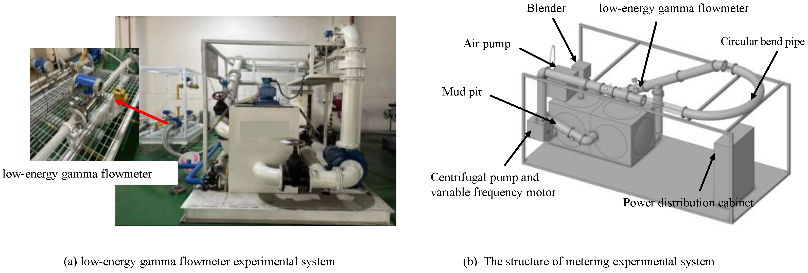
To simulate the multiphase flow conditions (gas, liquid, and solid) encountered during the drilling process, an experimental flow loop was established. As shown in Figure 5, the system integrates core components such as a blender, air pump, and centrifugal pump to ensure uniform multiphase mixing prior to measurement. Before conducting experiment, we used two mixing ratio modes of oil, gas, water, and solid. The mixing ratio mode one: gas phase ratio 6%, liquid phase ratio 90%, and solid phase ratio 4%. The mixing ratio mode two: gas phase ratio 5%, liquid phase ratio 85%, and solid phase ratio 10%.

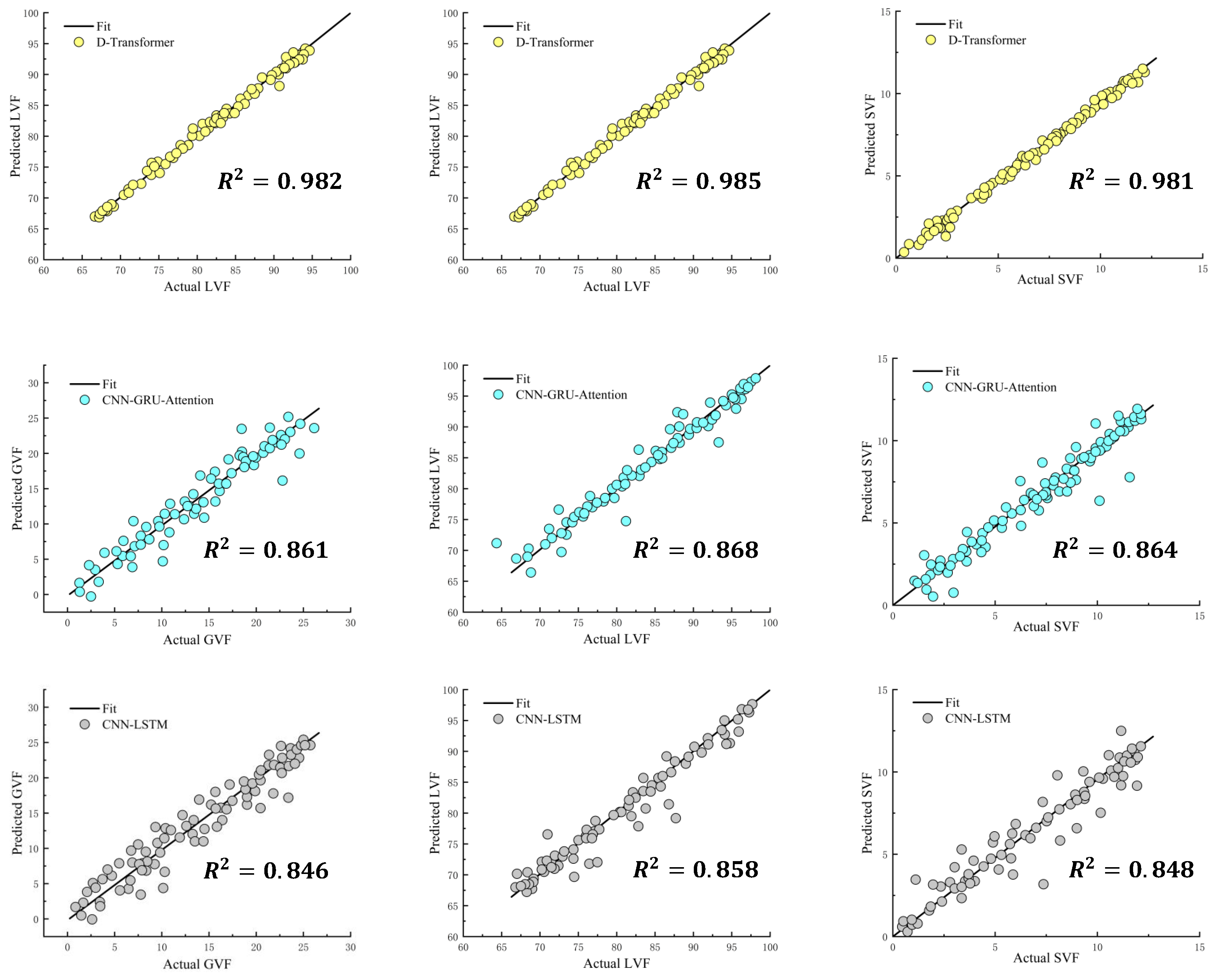
These two ratios are nominal initial mass-fraction feeding conditions rather than fixed instantaneous labels. During circulation, the instantaneous fractions vary continuously because of gas-injection fluctuations, pump-speed changes, gas compressibility, multiphase mixing, and solid settling. Consequently, the synchronized reference fractions measured during the dynamic experiments form a continuous distribution, which explains the continuous scatter in the prediction–reference comparison presented later.

All reference fractions were placed on a common mass-flow basis. The measured gas volumetric flow rate $q_g$ was converted to gas mass flow using the gas density at the pressure and temperature of the meter, while the liquid mass flow was measured directly by the Coriolis reference meter and the solid mass flow was obtained from the recorded solid feeding and mass balance:

$${\dot{m}}_g={\rho }_g(P_m,T_m)q_g,{\dot{m}}_l={\dot{m}}_{l,\mathrm{Coriolis}},{\dot{m}}_s={\dot{m}}_{s,\mathrm{balance}}.$$

After time synchronization over the same acquisition interval, the gas, liquid, and solid reference mass fractions were calculated as

$${\alpha }_k^{\mathrm{ref}}={\displaystyle \frac{{\dot{m}}_k}{{\dot{m}}_g+{\dot{m}}_l+{\dot{m}}_s}},k\in \{g,l,s\},$$

so that ${\alpha }_g^{\mathrm{ref}}+{\alpha }_l^{\mathrm{ref}}+{\alpha }_s^{\mathrm{ref}}=1$. This common mass basis is consistent with the mass fractions reported by the low-energy gamma flowmeter.

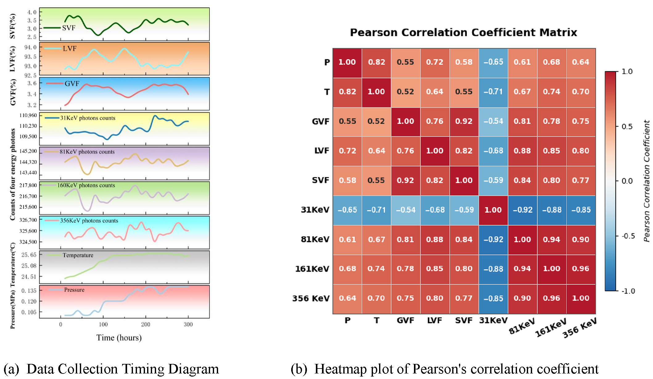
As shown in Figure 6, the data collected by our light-quantum mixed-phase measurement loop includes temperature, pressure, counts of various energy levels of light quanta, and phase fraction. This study mainly focuses on the soft correction of the accuracy of the phase fraction measured by the low-energy gamma flowmeter. Therefore, a correlation analysis was conducted on the collected data, to prove the rationality of using these parameters as inputs for the subsequent regression model.

The four photon-energy channels exhibit pairwise Pearson correlation coefficients of 0.85–0.96 because they share the same source intensity and are simultaneously affected by mixture density and phase composition. This high correlation does not make the channels physically identical: photons at 31, 81, 160, and 356 keV have different energy-dependent attenuation and penetration responses. All four channels were therefore retained to preserve complementary nonlinear attenuation information. Min–max scaling prevents a high-count channel from dominating numerically, while the attention layers learn channel-dependent contributions without requiring inversion of a correlated covariance matrix. The ridge-regression baseline reported below provides a regularized linear comparison under the same correlated inputs.

The data collected by the light-quantum mixed-phase measurement loop are saved into the data set $D=\left\{\right(X,Y\left)\right\}$. Y is the prediction output of the model. X contains 11 input variables: temperature, pressure, differential pressure, flow rate, the three phase-fraction readings produced by the low-energy gamma flowmeter, and the photon counts at 31, 81, 160, and 356 keV. The reference output Y contains the synchronized gas, liquid, and solid phase fractions. The input set is represented as follows.

$$X=\{x_{ij}^p\mid i=1,2,\cdots n_1;j=1,2,\cdots n_2\}$$

(9)

To avoid information leakage, complete experimental runs are assigned to the training, validation, and test subsets before interpolation, scaling, DBSCAN processing, or window generation. Small gaps are filled by linear interpolation using only adjacent observations within the same run and subset; irrecoverable segments are discarded. Min–max limits are then estimated from the training subset only and applied unchanged to the validation and test subsets. The scaling operation is

$$x^{\prime }={\displaystyle \frac{x-{min}_{\mathrm{train}}\left(x\right)}{{max}_{\mathrm{train}}\left(x\right)-{min}_{\mathrm{train}}\left(x\right)}}.$$

(10)

DBSCAN is fitted to the scaled training vectors. Candidate DBSCAN and Transformer hyperparameters are compared using validation-set mean $R^2$; the held-out test subset is not used for parameter selection or early stopping. After the parameters are fixed, the same preprocessing transformations are applied to the test subset, and windows are generated independently within each run.

Table 1. Model structure and training configuration.

Item	Setting
Input variables	11
Output variables	3 continuous phase fractions
Window length/sliding step	20/1
DBSCAN $\mathrm{Eps}$/$\mathrm{MinPts}$	0.6/10
Embedding dimension $d_{\mathrm{model}}$	32
Positional encoding	Learnable, $20\times 32$
Attention heads/encoder layers	8/12
Feed-forward dimension/dropout	128/0.1
Regression head	ResNet-MLP with compositional Softmax
Optimizer/initial learning rate	Adam/$1\times {10}^{-3}$
Batch size/maximum epochs	64/200
Loss function	Mean squared error
Early stopping	20 epochs without validation improvement
Hyperparameter criterion	Validation-set mean $R^2$

summarizes the model and training configuration. The same sequence length, experiment-wise partition, and optimization settings were used for the neural-network comparisons wherever applicable.

An experiment-wise five-fold outer partition is adopted for the time-series evaluation. Complete experimental runs, rather than individual time points or randomly shuffled windows, are assigned to five mutually exclusive blocks. In each outer fold, one block (approximately 4000 records) is held out for testing. Of the remaining four blocks, three (approximately 12,000 records) are used for parameter fitting and one (approximately 4000 records) is used for validation and early stopping. The validation role is rotated within the development blocks. Thus, temporally adjacent or overlapping windows from the same experiment cannot appear in different subsets. The counts in

Table 2. Data distribution for the experiment.

Data	Records per Fold
Total data	20,000
Training data	Approximately 12,000
Validation data	Approximately 4000
Testing data	4000

describe chronological records before window construction; for a run with $M_r$ valid records, the number of model samples is $M_r-W+1$, and sample totals are summed over runs.

The test block remains untouched during hyperparameter selection. After validation has selected $\mathrm{Eps}$, $\mathrm{MinPts}$, h, N, and $d_{\mathrm{model}}$, the resulting model is evaluated on the outer test block. The mean of the five outer test-fold results is reported as the final performance, thereby measuring generalization to complete experiments not used for fitting or tuning.

4.2. Comparative Experiment

This study is a continuous multi-output regression task rather than a classification task. Performance is therefore evaluated using the coefficient of determination ($R^2$) and root mean squared error (RMSE), not percentage classification accuracy. $R^2$ measures the explained variance, whereas RMSE measures the error in fraction units. Values of $R^2$ closer to one and RMSE closer to zero indicate better regression performance.

$$R^2=1-{\displaystyle \frac{{\sum }_{i=1}^N{\left(Y_{\mathrm{Pred}}\left(i\right)-Y_{\mathrm{Exp}}\left(i\right)\right)}^2}{{\sum }_{i=1}^N{\left(Y_{\mathrm{Exp}}\left(i\right)-{\overline{Y}}_{\mathrm{Exp}}\right)}^2}}$$

(11)

$$\mathrm{RMSE}={\left({\displaystyle \frac{{\sum }_{i=1}^N{\left(Y_{\mathrm{Pred}}\left(i\right)-Y_{\mathrm{Exp}}\left(i\right)\right)}^2}{N}}\right)}^{0.5}$$

(12)

The following neural, linear, ablation, and instrument baselines were evaluated using the same experiment-wise outer test folds.

CNN-GRU-Attention: The CNN-GRU-Attention model combines CNN, Gated Recurrent Units (GRU), and Attention mechanism. This model uses GRU to capture dependency features in the metric time series, and assigns different weights for features through attention mechanism. The CNN is used to predict the phase fractions data.

CNN-LSTM: The CNN-LSTM model combines CNN with Long Short-Term Memory Networks (LSTM). The LSTM is used to extract dependency features from metric time series data, and the CNN is used to predict phase fractions data.

No-DBSCAN (vanilla Transformer): DBSCAN is removed, while the 11 inputs, window length, Transformer, ResNet-MLP head, optimizer, and data partition are unchanged. This ablation isolates the contribution of density-based denoising.

No-ResNet: DBSCAN and the Transformer encoder are retained, but the residual regression head is replaced by an ordinary two-layer MLP with the same three-component Softmax output. This ablation isolates the contribution of the residual decision module.

Ridge regression: the same normalized 20-point input window is flattened and passed to a regularized multivariate linear regression model. This provides a simple regression baseline while controlling the instability caused by the correlated photon-energy channels.

Uncorrected flowmeter: the raw gas, liquid, and solid fractions reported by the low-energy gamma flowmeter are compared directly with the synchronized references, without data-driven correction.

Table 3. Performance comparison of different models for phase fraction prediction.

Model	Phase	${\mathit{R}}^2$	RMSE
D-Transformer	Gas	0.982	0.0134
	Liquid	0.985	0.0122
	Solid	0.981	0.0138
No-ResNet	Gas	0.974	0.0161
	Liquid	0.978	0.0148
	Solid	0.971	0.0170
No-DBSCAN	Gas	0.956	0.0208
	Liquid	0.960	0.0197
	Solid	0.954	0.0214
CNN-GRU-Attention	Gas	0.861	0.0373
	Liquid	0.868	0.0363
	Solid	0.864	0.0369
CNN-LSTM	Gas	0.846	0.0396
	Liquid	0.858	0.0378
	Solid	0.848	0.0390
Ridge regression	Gas	0.792	0.0456
	Liquid	0.811	0.0433
	Solid	0.784	0.0465
Uncorrected flowmeter	Gas	0.623	0.0613
	Liquid	0.651	0.0589
	Solid	0.596	0.0636

shows a monotonic improvement from the uncorrected instrument and ridge regression to the temporal neural models and the complete D-Transformer. Removing ResNet reduces the three $R^2$ values to 0.974, 0.978, and 0.971, whereas removing DBSCAN reduces them further to 0.956, 0.960, and 0.954. Thus, both the residual head and DBSCAN contribute, and the larger no-DBSCAN degradation supports the proposed adhesion-noise treatment. Relative to the uncorrected flowmeter, D-Transformer reduces RMSE by 78.1%, 79.3%, and 78.3% for the gas, liquid, and solid fractions, respectively. The complete model achieves a maximum $R^2$ of 0.985 and a minimum RMSE of 0.0122. Figure 7 compares the synchronized reference fractions with the D-Transformer predictions.

4.3. Key Parameters Influence

4.3.1. The DBSCAN Parameters Influence

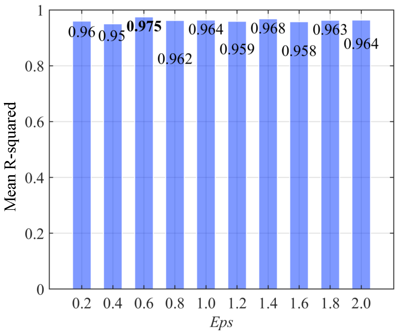
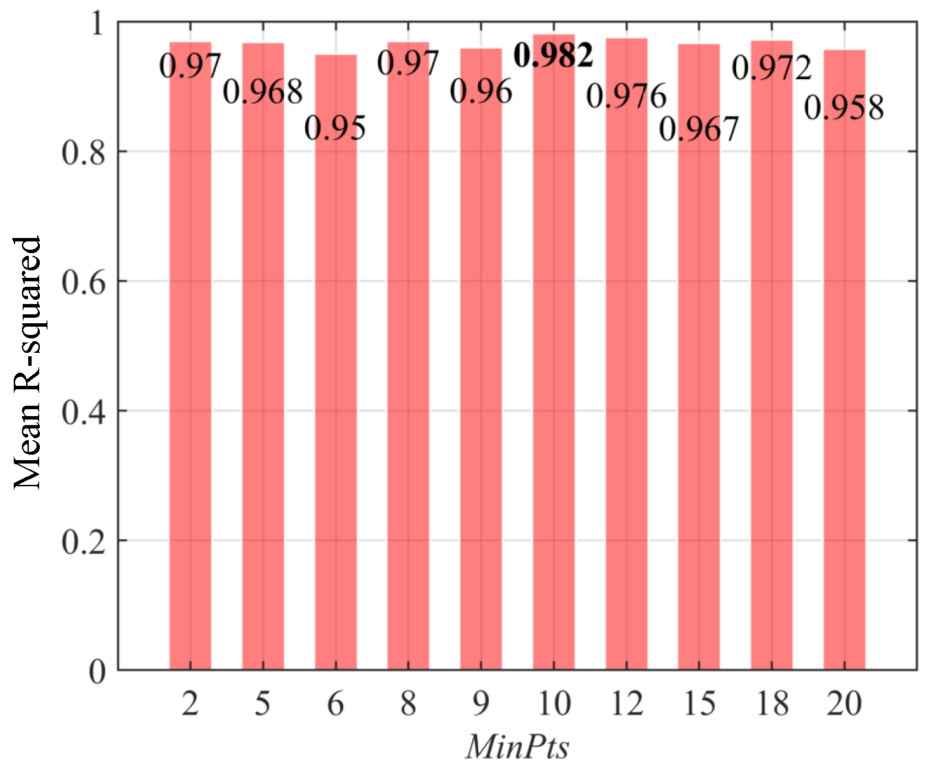
In DBSCAN, $\mathrm{Eps}$ and $\mathrm{MinPts}$ control neighborhood size and the minimum local density. Candidate values were compared using mean $R^2$ on the validation subsets only; the outer test subsets were not inspected during tuning. Figure 8 shows the validation mean $R^2$ for $\mathrm{Eps}\in \{0.2,0.4,\dots ,2.0\}$, with the maximum $R^2=0.975$ at $\mathrm{Eps}=0.6$. Figure 9 shows the corresponding search over $\mathrm{MinPts}\in \{2,5,6,8,9,10,12,15,18,20\}$, with the maximum validation $R^2=0.982$ at $\mathrm{MinPts}=10$.

4.3.2. The Transformer Parameters Influence

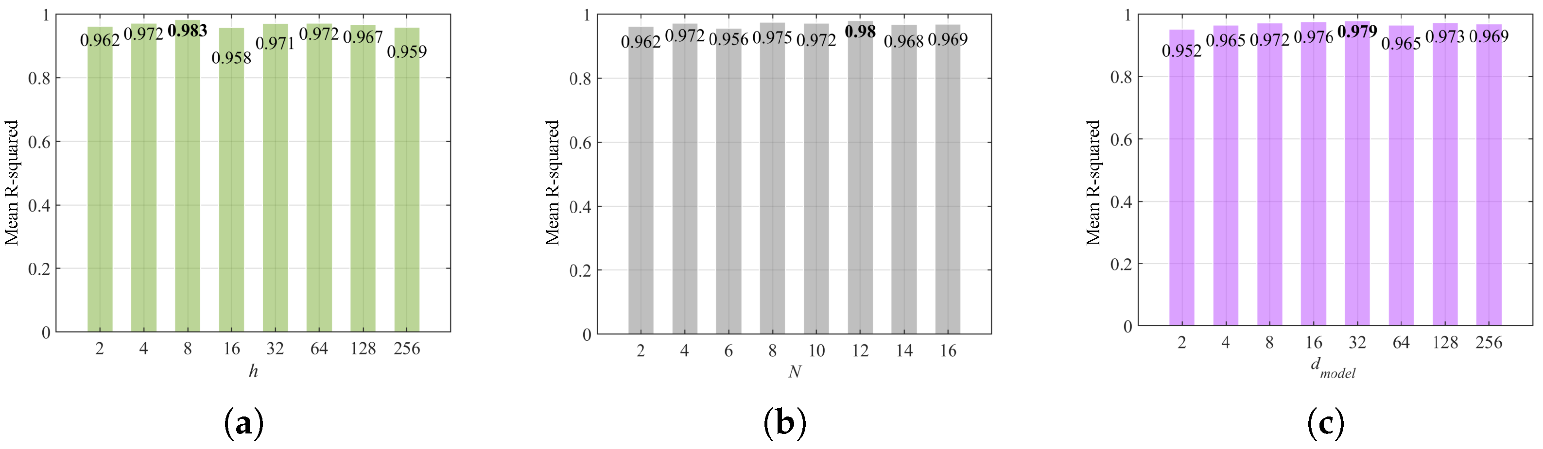
The Transformer hyperparameters were selected by the same validation-only procedure. The candidates were $h\in \{2,4,8,16,32,64,128,256\}$ attention heads, $N\in \{2,4,6,8,10,12,14,16\}$ encoder layers, and $d_{\mathrm{model}}\in \{2,4,8,16,32,64,128,256\}$. As shown in Figure 10, the highest validation mean $R^2$ values are 0.983 at $h=8$, 0.980 at $N=12$, and 0.979 at $d_{\mathrm{model}}=32$. The selected configuration is therefore $\{h=8,N=12,d_{\mathrm{model}}=32\}$. These searches do not use the held-out test data; the final test-fold results are reported only after the configuration is fixed.

4.4. Case Analysis in Practice

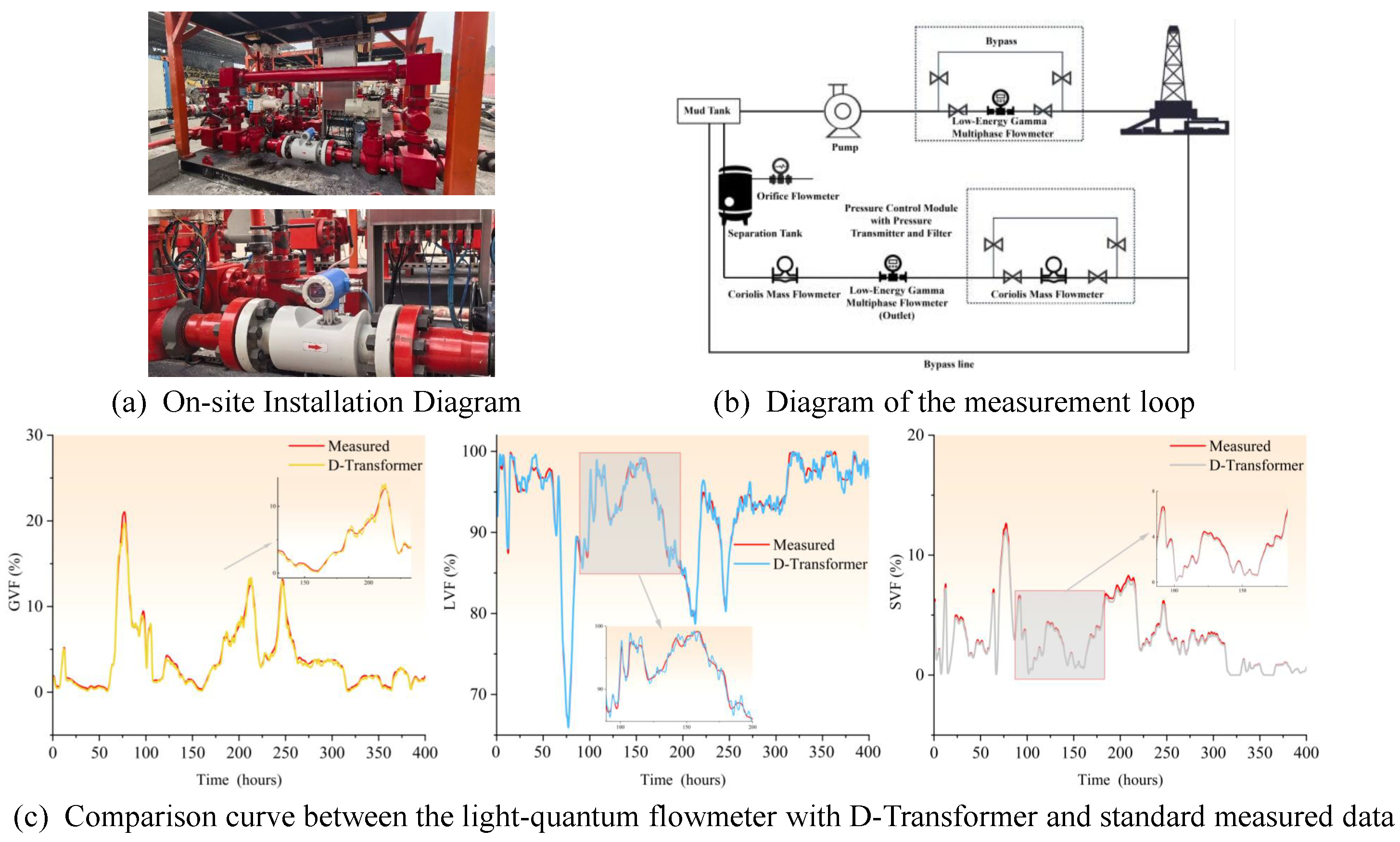
To verify that this algorithm has practical engineering value, we selected an operating well in Sichuan for a field experiment. The field experiment was conducted on a drilling platform in Sichuan in August 2024. The low-energy gamma flowmeter was installed in the straight pipe section at the downstream outlet of the choke manifold, approximately 3 m away from the choke valve, to measure the outlet flow rate of the drilling fluid. The on-site installation diagram is shown in Figure 11a. The fluid is a gas-liquid-solid three-phase mixture after throttling and pressure reduction. During data collection, the well depth was approximately 5800 m, and the drilling fluid density was 1.2. Due to geological factors, it contains associated gas. Therefore, in the gas-liquid-solid three-phase mixture, the gas phase is associated gas, the liquid phase is water-based drilling fluid, and the solid phase consists of barite and some high molecular polymers contained in the drilling fluid. The on-site loop consists of a mud pump, a mud tank, the low-energy gamma flowmeter under evaluation, a separation tank, a high-precision Coriolis mass flowmeter, and an orifice flowmeter. As shown in Figure 11b, the multiphase mixture first passes through the low-energy gamma flowmeter and then enters the separation tank, where gravity settling separates gas from the liquid-solid stream. The orifice meter provides gas volumetric flow, which is converted to mass flow using gas density at the line pressure and temperature. The Coriolis meter provides liquid mass flow directly, and the solid mass flow is obtained from the recorded feed and drilling-fluid mass balance. The three synchronized mass-flow references are normalized using the same mass-fraction equations given above, ensuring that the reference gas, liquid, and solid fractions are on a common basis and sum to unity. We encapsulated the D-Transformer algorithm into a module and integrated it into the embedded edge hardware of the low-energy gamma flowmeter to perform real-time calibration of the phase fraction of the low-energy gamma flowmeter. As shown in Figure 11c, compared with the reference data, the corrected low-energy gamma flowmeter satisfies the phase-fraction error threshold for managed-pressure-drilling field application and can provide data support for early kick detection, pressure-parameter optimization, and wellbore safety decisions.

5. Conclusions

This article has proposed the D-Transformer regression framework for correcting phase-fraction errors in a low-energy gamma flowmeter. Under leakage-controlled experiment-wise evaluation, the complete model obtained $R^2$ values of 0.982, 0.985, and 0.981 for the gas, liquid, and solid fractions. The no-ResNet and no-DBSCAN ablations verify the contributions of the residual regression head and density-based detector-noise removal, respectively. D-Transformer also outperforms CNN-GRU-Attention, CNN-LSTM, ridge regression, and the uncorrected flowmeter. Learnable positional encoding captures within-window order, the compositional Softmax guarantees non-negative fractions summing to unity, and the common mass-flow reference construction closes the measurement balance. However, the D-Transformer algorithm has potential shortcomings. For example, when encountering segmented multiphase flow, the effective information is discontinuous within the metering time-series data, and the D-Transformer model may fail due to this discontinuity. In the future, we will research deep-learning metrological calibration methods suitable for various flow regimes such as slug flow, bubbly flow, and annular flow.

References

1. Agwu, O.E.; Okoro, E.E.; Sanni, S.E. Modelling oil and gas flow rate through chokes: A critical review of extant models. J. Pet. Sci. Eng. 2022, 208, 109775. [Google Scholar] [CrossRef] [Scilit]
2. Cai, J.; Jiao, X.; Wang, H.; He, W.; Xia, Y. Multiphase fluid-rock interactions and flow behaviors in shale nanopores: A comprehensive review. Earth-Sci. Rev. 2024, 257, 104884. [Google Scholar] [CrossRef] [Scilit]
3. Song, K.; Liu, Y. A compact x-ray system for two-phase flow measurement. Meas. Sci. Technol. 2018, 29, 025305. [Google Scholar] [CrossRef] [Scilit]
4. Basahel, A.; Sattari, M.A.; Taylan, O.; Nazemi, E. Application of Feature Extraction and Artificial Intelligence Techniques for Increasing the Accuracy of X-ray Radiation Based Two Phase Flow Meter. Mathematics 2021, 9, 1227. [Google Scholar] [CrossRef] [Scilit]
5. Taylan, O.; Sattari, M.A.; Essoussi, I.E.; Nazemi, E. Frequency Domain Feature Extraction Investigation to Increase the Accuracy of an Intelligent Nondestructive System for Volume Fraction and Regime Determination of Gas-Water-Oil Three-Phase Flows. Mathematics 2021, 9, 2091. [Google Scholar] [CrossRef] [Scilit]
6. Bilgic, A.M.; Kunze, J.W.; Stegemann, V.; Hogendoorn, J.; Cerioni, L.; Zoeteweij, M. Multiphase flow metering with nuclear magnetic resonance. TM—Tech. Mess. 2015, 82, 539–548. [Google Scholar] [CrossRef] [Scilit]
7. Meribout, M. Optimal Design for a Portable NMR- and MRI-Based Multiphase Flow Meter. IEEE Trans. Ind. Electron. 2019, 66, 6354–6361. [Google Scholar] [CrossRef] [Scilit]
8. Meribout, M.; Sonowan, S. Optimal Halbach Magnet Array Design for Portable NMR Targeting Multiphase Flow Metering Applications. IEEE Trans. Magn. 2019, 55, 4001207. [Google Scholar] [CrossRef] [Scilit]
9. Meribout, M.; Shehzad, F.; Kharoua, N.; Khezzar, L. Gas-liquid two-phase flow measurement by combining a Coriolis flowmeter with a flow conditioner and analytical models. Measurement 2020, 163, 107826. [Google Scholar] [CrossRef] [Scilit]
10. Fadaei, M.; Ameli, F.; Hashemabadi, S.H. Investigation on different scenarios of two-phase flow measurement using Orifice and Coriolis flow meters: Experimental and modeling approaches. Measurement 2021, 175, 108986. [Google Scholar] [CrossRef] [Scilit]
11. Chowdhury, W.S.; Yan, Y.; Coster-Chevalier, M.A.; Liu, J. Mass Flowrate Measurement of Slurry Using Coriolis Flowmeters and Data Driven Modeling. IEEE Trans. Instrum. Meas. 2024, 73, 7503612. [Google Scholar] [CrossRef] [Scilit]
12. Zeeshan, Z.; Zuccarelli, C.E.; Acero, D.O.; Marashdeh, Q.M.; Teixeira, F.L. Enhancing Resolution of Electrical Capacitive Sensors for Multiphase Flows by Fine-Stepped Electronic Scanning of Synthetic Electrodes. IEEE Trans. Instrum. Meas. 2019, 68, 462–473. [Google Scholar] [CrossRef] [Scilit]
13. Sun, S.; Lu, X.; Xu, L.; Cao, Z.; Sun, J.; Yang, W. Real-Time 3-D Imaging and Velocity Measurement of Two-Phase Flow Using a Twin-Plane ECT Sensor. IEEE Trans. Instrum. Meas. 2021, 70, 4504210. [Google Scholar] [CrossRef] [Scilit]
14. da Mota, F.R.; Pagano, D.J.; Stasiak, M.E. Water Volume Fraction Estimation in Two-Phase Flow Based on Electrical Capacitance Tomometry. IEEE Sens. J. 2018, 18, 6822–6835. [Google Scholar] [CrossRef] [Scilit]
15. Bin, X.U.; Chen, J.; Guo, P.; Jingyang, L.I. Device for Measuring Flow Rate of Wet Gas Based on an Exempt Radioactive Source. U.S. Patent Application No. 16/335,263, 20 August 2020. [Google Scholar]
16. Luchi, D.; Rodrigues, A.L.; Varejao, F.M. Sampling approaches for applying DBSCAN to large datasets. Pattern Recognit. Lett. 2019, 117, 90–96. [Google Scholar] [CrossRef] [Scilit]
17. Vaswani, A.; Shazeer, N.; Parmar, N.; Uszkoreit, J.; Jones, L.; Gomez, A.N.; Kaiser, Ł.; Polosukhin, I. Attention is all you need. In Proceedings of the Advances in Neural Information Processing Systems, Long Beach, CA, USA, 4–9 December 2017. [Google Scholar]
18. Zhang, C.; Benz, P.; Argaw, D.M.; Lee, S.; Kim, J.; Rameau, F.; Bazin, J.C.; Kweon, I.S. ResNet or DenseNet? Introducing Dense Shortcuts to ResNet. In Proceedings of the 2021 IEEE Winter Conference on Applications of Computer Vision WACV, Virtual, 5–9 January 2021; pp. 3549–3558. [Google Scholar] [CrossRef] [Scilit]
Figure 1. The low-energy gamma flowmeter.
Processes 14 02644 g001
Figure 2. The photon absorption principle for oil, gas, water, and solid substances.
Processes 14 02644 g002
Figure 3. The overall architecture of the improved transformer for phase fractions correction.
Processes 14 02644 g003
Figure 4. Multi-head attention (MHA).
Processes 14 02644 g004
Figure 5. Low-energy gamma flowmeter metering experimental loop.
Processes 14 02644 g005
Figure 6. Data collection and correlation analysis.
Processes 14 02644 g006
Figure 7. Comparison of predicted and reference phase fractions (GVF, LVF, and SVF).
Processes 14 02644 g007
Figure 8. Validation mean R 2 for different DBSCAN Eps values. The bold number indicates the selected optimum.
Processes 14 02644 g008
Figure 9. Validation mean R 2 for different DBSCAN MinPts values. The bold number indicates the selected optimum.
Processes 14 02644 g009
Figure 10. Validation mean R 2 for different Transformer hyperparameters. (a) Number of attention heads h; (b) number of encoder layers N; (c) embedding dimension d model . The bold numbers indicate the selected optima.
Processes 14 02644 g010
Figure 11. Experimental device and experimental results of the on-site drilling return-fluid measurement loop. (a,b) Physical installation and schematic of the on-site measurement loop; (c) comparison of the predicted phase fractions (GVF, LVF, and SVF) with the synchronized reference values obtained from the separation and reference-metering system.
Processes 14 02644 g011