Adaptive Connectivity and Robust Plane Extraction from Microseismic Event Clouds: A Systematic Benchmark and Conditional Case Study

Abstract

Two-meter-scale true-triaxial hydraulic-fracturing models involve a large monitoring volume, strongly nonuniform microseismic event densities, and substantial vibration and background noise, making conventional fixed-scale clustering or direct geometric fitting prone to cluster fragmentation, event-band mixing, and low-support false planes. To address these limitations, this study proposes an automatic workflow for extracting dominant event planes from noisy microseismic point clouds. After quality control and spatial-boundary screening, nearest-neighbor statistics are used for adaptive density analysis, followed by support-first RANSAC plane fitting and PCA-based parameter refitting. Parameter sensitivity, null-model testing, and subsampling stability are further used to evaluate robustness. Extended synthetic tests demonstrate that the workflow can identify multiple planes under varying noise levels, event densities, plane spacing, and localization errors, while stage constraints are particularly important for separating spatially overlapping event bands. The method was then applied to three 2 m × 2 m × 1 m tight-sandstone fracturing experiments. For each specimen, 3200 high-quality candidate events were retained from approximately 10,000 located events. The extracted dominant subhorizontal event planes showed support fractions of 12.38%, 15.19%, and 11.94%, dips of 0.97°, 0.59°, and 1.83°, and RMS residuals of 10.96, 10.43, and 11.12 mm, respectively. The results indicate that the proposed workflow can consistently extract coherent dominant event planes from high-noise, nonuniform microseismic datasets in large-scale physical models. These planes represent dominant spatial structures of the located events and should not be interpreted directly as actual opened or conductive hydraulic-fracture surfaces.

1. Introduction

Hydraulic-fracture interpretation requires a distinction between observations of rock response and the geometry assigned to those observations. A table of located acoustic-emission or microseismic events provides discrete positions, not a directly observed fracture surface. Even a well-fitted plane can contain mechanically different sources, while some parts of an opened fracture may be weakly sampled. Laboratory monitoring is useful for constraining fracture development, but geometrical extraction from an event cloud and independent physical validation remain separate tasks [1,2]. This study addresses the first task and explicitly limits what the available experimental data establish about the second.

True-triaxial experiments in tight sandstone–coal interbeds show that weak interfaces can alter fracture trajectories [3], while Frash et al. documented branching, coalescence and reorientation in three-dimensional laboratory fractures [4]. At the reservoir scale, Li et al. combined seismic attributes to identify faults of different scales in shale formations [5]. These studies motivate scale-aware interpretation and the use of complementary observations, but neither field-scale attribute maps nor laboratory fracture patterns provide event-wise ground truth for the present coordinate tables.

Density-based fracture identification and robust multi-plane estimation are established approaches. Xue et al. incorporated time–spatial constraints into density-based fracture identification [2], and Yu et al. developed a multi-model fitting approach for microseismic fracture-network extraction [6]. DBSCAN defines clusters through density connectivity [7,8]; hierarchical density methods provide alternatives when one global density level is inadequate [9,10]. RANSAC already prioritizes consensus support over isolated low-residual hypotheses [11]. Neither the use of these components nor a maximum-consensus objective is claimed here as a new algorithmic principle.

Multi-model fitting also extends beyond density-based grouping. J-Linkage groups observations by their preferences for sampled model hypotheses [12]. In a different engineering setting, Zhao et al. used DBSCAN to group carbon sources and sinks before optimizing a CCUS pipeline network [13]. The latter is an example of spatial-data organization, not a microseismic fracture-reconstruction benchmark. Together, these approaches emphasize the need to distinguish candidate grouping from subsequent model estimation or engineering optimization.

The methodological question is instead whether a specified integration adds identifiable value, and under what information conditions. An underscaled fixed radius is an informative transfer-failure example, but is not a sufficient competitor for an adaptive method. Likewise, a clustering stage that returns all observations as one group cannot be credited with separating fractures in that case. Valid stage information may prevent undesirable cross-stage merging, but this is additional information, not a gain attributable solely to density adaptation. Tests must therefore separate density-scale selection, local-radius adaptation, robust fitting and stage availability.

Three further distinctions motivate the present evaluation. First, the precision with which coordinates are stored is not their localization accuracy. Velocity-model uncertainty can affect both event locations and their estimated uncertainties, as demonstrated by Gesret et al. [14]. Second, a low inlier residual partly follows from imposing an inlier-distance threshold, and is not independent ground-truth verification. Third, a plane with unusually high support relative to a spatially uniform reference may cease to be unusual after the reference preserves a strong observed Z-coordinate concentration. These distinctions are especially important for curated archives whose original waveforms and selection metadata are unavailable.

Recent data-driven seismic studies further broaden this methodological context. Mahzad and Bagheri used a U-Net-based framework to reconstruct missing geological events and structural patterns in real-life 3D post-stack seismic images [15], while Esmaeili et al. integrated multiple seismic attributes with a hybrid MLP-SVM framework for automated fault detection [16]. These studies operate on seismic images rather than laboratory microseismic event clouds, but they illustrate a broader trend toward automated extraction of geological structure from complex, noisy and incomplete geophysical observations. The present study addresses a related but distinct task: extracting dominant planar consensus structures directly from discrete located-event coordinates.

The revised contribution is an explicitly specified connectivity-and-fitting workflow, a matched-kernel comparison against no clustering, two data-scaled fixed-radius baselines and HDBSCAN, and a validation protocol that reports conditional successes and failures. Synthetic clouds supply known event and plane labels; experimental subsets supply only positions and time. All numerical results below were recomputed with a newly developed revision-stage implementation. They replace, rather than purport to exactly reproduce, results from the unavailable original paper-specific implementation. No claim is made that the workflow is parameter-free, that adaptive connectivity is universally superior, or that the experimental outputs recover complete hydraulic-fracture networks.

2. Materials and Methods

2.1. Specimens, Loading and Injection Configuration

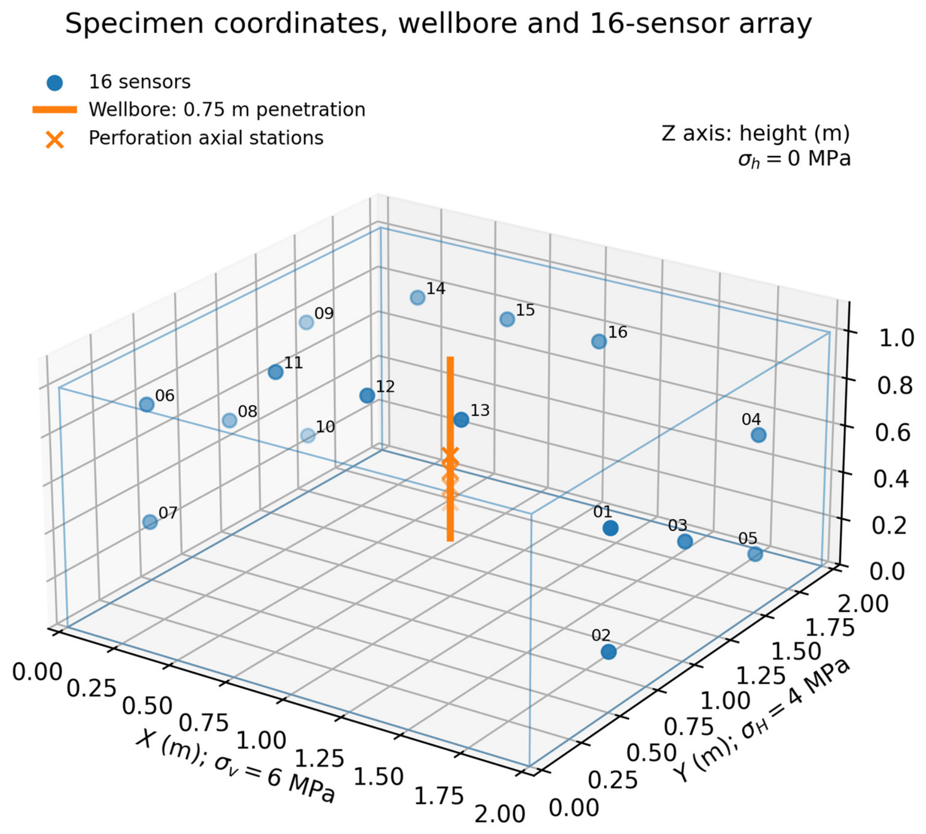
The experiments used nominal 2 m × 2 m × 1 m tight-sandstone analog blocks with a central wellbore in a true-triaxial loading apparatus. The submitted experimental description records a cement–quartz sand–water mass ratio of 1:0.50:0.25 and 28-day curing; no new material-property measurements were available for this revision. The coordinate origin is a lower specimen corner, with X and Y spanning 0–2 m and Z spanning 0–1 m. Coordinates describe the specimen, not geographic north and vertical stress directions in situ.

The experimental team clarified the operating conditions during revision (

Table 1. Experimental conditions clarified by the experimental team.

Item	S1	S2	S3
Nominal injection rate (m3/min)	0.2	0.3	0.4
Nominal fluid viscosity (mPa·s)	5	5	5
Fluid system	Guar gum	Guar gum	Guar gum
Applied σh–σH–σv (MPa)	0–4–6	0–4–6	0–4–6
Proppant/temporary plugging	Neither	Neither	Neither
Archived candidate events	3200	3200	3200

). The nominal guar-gum-fluid viscosity was 5 mPa·s; no proppant or temporary plugging was used. Applied stresses, stated in the experimental convention as σh–σH–σv, were 0–4–6 MPa. In specimen coordinates, X carries the reservoir-equivalent σv = 6 MPa, Y carries σH = 4 MPa, and Z carries σh = 0 MPa. Thus, the label σv does not denote the geometric Z axis of the rotated physical model. The values are reported applied loads; an unmeasured pore-pressure correction is not introduced.

The wellbore is centered at (X,Y) = (1,1) m, parallel to Z, and penetrates 0.75 m below the upper surface, terminating at Z = 0.25 m. Four 10 mm perforations follow a 90° phasing sequence with 66 mm axial spacing. Their group midpoint is at Z = 0.50 m, giving nominal axial stations Z = 0.401, 0.467, 0.533 and 0.599 m by symmetry. These positions are derived from the supplied midpoint and spacing, rather than from an independent dimensional survey. The absolute azimuth of the first hole was not recorded in the available information; Figure 1 therefore marks axial stations without inventing azimuthal registration. The three experimental specimens are hereafter denoted S1, S2, and S3, respectively.

Each injection-rate condition has one specimen (n = 1); specimen order and support fractions are not evidence of a rate trend. The supplied nominal perforation density was 16 holes/m; the reciprocal of the specified 66 mm pitch is approximately 15.2 m⁻¹. Geometry calculations use the explicit pitch, not an assumed exact density of 16 m⁻¹.

2.2. Monitoring, Retrospective Curation and Evidence Boundaries

The experimental team reports a DS-5-series acoustic-emission/microseismic acquisition system (Beijing Soft Island Times, Beijing, China) with 16 synchronous channels sampled at 3 MHz per channel. Locations were calculated from multi-channel P-wave first arrivals using a fixed homogeneous P-wave speed of 2350 m/s. Independent formal S-wave picks were not made, so the procedure is not described as joint P/S localization. These acquisition and localization settings are retrospective experimental information, not parameters newly estimated from the archived coordinate tables.

According to the experimental team’s retrospective account, each specimen initially had approximately ten thousand located candidate events; exact original counts are no longer recoverable. Events of poor localization quality and positions outside the specimen were excluded. Quality was judged jointly from participating-channel count, localization error and arrival-time residual. The remaining candidates were quality-ranked and a fixed-size set of 3200 events was retained per specimen to limit computational size and maintain a common comparison scale. This was a quality-selected subset, not random downsampling, and not the complete detected-event record.

The available tables contain only EventID, X_m, Y_m, Z_m and Time_s. They retain neither the quality indicators nor their ranking scores. Exact screening thresholds, the rule for combining the three indicators, the complete pre-screening tables, the screening script, raw waveforms and original pick records are unavailable. Consequently, the historical selection cannot be independently reproduced. A high-quality location also need not be a fracture source: the experimental team reports substantial vibration/background contamination after curation. No event-wise vibration-versus-fracture labels are available. In this paper, “non-consensus” means outside the fitted plane’s tolerance, not proven physical noise.

The revised input audit checks identifiers, finite coordinates, bounds, duplicate triplets, numerical precision and time ordering. The three 3200-event subsets are the sole experimental inputs. A fourth uploaded workbook was inspected for dataset identification but is not included as an additional experimental case. The supplied code package contains monitoring and localization utilities but no recovered implementation of the paper’s adaptive-clustering benchmark. Contemporary utilities for other specimens are therefore not treated as proof of the historical processing of S1–S3.

2.3. Revision-Stage Implementation and Parameter Provenance

A separate reference implementation, REVISION_REFERENCE_V2_20260907, was created for this revision. The missing local-radius formula, the plane-matching rule and all random seeds are now explicit. The submission-stage constants 1.15, quantile 0.72, k = 7, radius limits, 20 mm tolerance and 7°/25 mm merge gates are retained as declared starting values and subjected to sensitivity tests; their original tuning history cannot be recovered. In particular, the submission itself states that the real-data radius bounds had been recalibrated from observed neighbor distances. The revision does not retroactively call this calibration a blind, frozen validation.

New simulation geometry, synthetic uncertainty generation and evaluation rules are documented as revision-stage design choices. They were held fixed for the reported run set; this is not a claim of preregistration or independence from the earlier review discussion. The experimental pipeline has no stage labels or event-specific errors and therefore disables those optional modules. Analytical verification here begins at the retained coordinate subsets or at the new synthetic generator, not at the lost experimental waveforms. The revision-stage calculations were performed using Python 3.13.5, NumPy 2.3.5, SciPy 1.17.0, scikit-learn 1.8.0, and Numba 0.65.1. The principal implementation settings and their provenance are summarized in

Table 2. Principal implementation settings and their status.

Setting	Value/Definition	Status
Neighbor scale	k = 7; Q0.72; multiplier 1.15	Submission-stage starting values; swept in revision
Global radius bounds	Real: 0.030–0.220 m; synthetic: 0.012–0.060 m	Real bounds previously data-calibrated; not a universal scale
Event-specific radius	clip [εg d7,i/Q0.72(d7), 0.75εg, 1.35εg]	Explicit revision-stage completion of underspecified rule
Core/retained group	MinPts = 7, including self; group size ≥ 30	Operational thresholds; sensitivity reported
RANSAC effort	3000 distinct-point triples per fitted model	Identical kernel and per-fit budget across comparisons
Base inlier tolerance	Real: 20 mm; new synthetic: 8 mm	Real sweep: 10, 15, 20, 25, 30 mm
Coplanar repair	Normal angle ≤ 7°; symmetric separation ≤ 25 mm	Synthetic sensitivity at 5–10° and 15–35 mm
Primary real-case random seed	20260907	Not selected by maximizing the reported support
Legacy 8% acceptance gate	Not used in revised spatial or temporal inference	Continuous support and explicit null tests replace this gate

.

2.4. Adaptive Connectivity and Candidate Grouping

Let xi be an event position and d7,i its distance to the seventh other event in the current group. All distances remain in physical meters; coordinate standardization that would distort plane angles is not applied. For available process-stage labels, grouping is performed within each labeled stage. For experimental tables without such labels, all events initially belong to one group. The global and local radii are

ε_g = clip [1.15 Q_0.72(d₇), ε_min, ε_max].

(1)

ε_i = clip [ε_g d_7,i/Q_0.72(d₇), 0.75ε_g, 1.35ε_g].

(2)

Events i and j are neighbors when ‖xi − xj‖₂ ≤ (εi + εj)/2. A core event has at least seven neighbors, counting itself. Candidate groups are connected components of the core-only graph. A non-core border event is assigned to an adjacent core component by the smallest normalized separation 2‖xi − xj‖₂/(εi + εj), with component index as a deterministic tie-breaker. A point without a core neighbor is labeled as unassigned; components with fewer than 30 events are also removed. Border-to-border chains cannot bridge core components. This is a fully specified variable-radius density rule, rather than an assertion that standard DBSCAN itself has event-specific radii [7,8]. Pseudocode is provided in Supplementary Section S2.

2.5. Support-First Plane Estimation, Refitting and Repair

A plane is represented by a unit normal n and intercept d, with nᵀx + d = 0. Three distinct, non-collinear candidate events generate a RANSAC hypothesis; nearly degenerate triples with cross-product norm below 10⁻¹² m² are skipped. The orthogonal residual is ri = |nᵀxi + d|. A hypothesis is ranked lexicographically by weighted inlier support and then by residual compactness:

I = {i: r_i ≤ τ_i};   C = Σ_i∈I w_i;   T = Σ_i∈I w_i [1 − (r_i/τ_i)²].

(3)

The hypothesis with the largest C is retained; T resolves support ties. A single weighted principal-component refit then estimates the normal from the smallest covariance eigenvector [17], and membership is recomputed against the refitted plane. The reported support is this post-refit membership, which can differ from the winning pre-refit support. The normal sign is set by nz ≥ 0. The reported center is the post-refit consensus centroid projected onto the reported plane. This maximum-consensus approach is consistent with the established RANSAC principle [11]; it is not presented as a new objective. Local optimization of RANSAC hypotheses has been studied explicitly [18]; the present implementation instead retains the stated single-refit rule and does not implement iterative LO-RANSAC.

Real cases use τi = 0.020 m and wi = 1. Missing localization errors are not treated as measured zero uncertainty. Only synthetic weighted runs use τi = max(0.008 m, 2σi) and wi = 1/[1 + (σi/0.003 m)²]. Synthetic uncertainties and weights are generated independently of whether an event is labeled as background; they do not encode the answer. For anisotropic synthetic errors, σi is the largest imposed coordinate standard deviation, a conservative scalar approximation rather than a full covariance-aware model.

Experimental comparisons report the strongest plane per retained group and then the strongest group-level result. Its primary support is the number of eligible inliers divided by the full input count; excluded points are not silently restored to the numerator. Synthetic multi-model runs sequentially remove a plane’s inliers, require at least 30 inliers for an accepted model, and stop when insufficient points remain or six models have been accepted within a candidate component. Coplanar fragments may merge only within the same available stage when their normal angle is at most 7° and both center-to-other-plane distances are at most 25 mm. A weighted PCA refits the union. This repair represents planar fragments, not curvature or branching.

2.6. Comparator Design

All schemes use the same fitting/refitting kernel. R uses no clustering. F transfers ε = 0.060 m and is explicitly a scale-transfer stress test. G uses standard DBSCAN with a single ε equal to Equation (1), isolating global scale selection from local adaptation. K uses a deterministic k-distance knee: sort d7, normalize the sorted values and their ranks to [0,1], choose the largest vertical distance below the end-to-end chord, and clip the corresponding distance to the same domain-specific bounds. This label-free rule is a conventionally motivated scale estimate, not a claim of globally optimal tuning. Knee-detection work provides methodological context [19]; this chord-distance rule is not the complete Kneedle algorithm. A uses Equations (1) and (2). H uses HDBSCAN with a minimum cluster size of 30, seven minimum samples and a permitted single cluster [9,10,20].

Synthetic ablations additionally include stage-constrained R (SR), stage-constrained A (SA), and stage-constrained A with uncertainty-aware tolerance and weights (SW). SR is important because it separates the benefit of stage information from the benefit of adaptive density grouping. Common per-fit budgets do not imply identical total runtimes when different methods return different numbers of groups. No computational-speed superiority is asserted, and the HDBSCAN configuration is a transparent comparator rather than an exhaustive optimization of that algorithm.

2.7. New Synthetic Benchmark and Failure Scenarios

The simulation suite separates data-generating scenarios, evaluated methods and performance measures, consistent with the reporting framework discussed by Morris et al. [21]. The old deterministic benchmark coordinates and code could not be recovered. A new, disclosed reference family therefore preserves its 270 signal events and its 360-event total at 25% background, but not its unknown original geometry. Three labeled planes receive 90 signal events each within a nominal 0.4 m × 0.4 m × 0.3 m domain. Their base centers are (0.15,0.15,0.12), (0.25,0.25,0.13) and (0.20,0.20,0.21) m. Base normals are the normalized vectors (0.7,0.1,0.5), (0.15,0.9,0.3) and (0.1,−0.2,1). A small independent normal perturbation varies in orientation between reference realizations. Signal points are uniform on 0.20 m × 0.20 m planar patches before location error is added.

For ordinary cases, event-specific isotropic standard deviations are sampled uniformly from 1.5 to 5.5 mm. Noise fraction η is defined relative to all events: noise = round [270η/(1 − η)]. Uniform background is sampled from the nominal domain. Five fractions, 10%, 20%, 30%, 40% and 50%, are generated with seeds 1000–1019 in each scenario. An additional 20 reference realizations use 25% noise. There are 1120 clouds and 10,080 method evaluations, not thousands of independent physical specimens.

Nine planar scenarios comprise the reference family, intersecting planes, parallel planes separated by 15 mm, unequal patch sizes, imbalanced populations of 180/60/30, anisotropic coordinate errors, a clustered-background component, missing stages and 30% incorrect stage labels. Two further scenarios use curved sheets and V-shaped branched sheets as out-of-model tests. Their surface-family labels permit assignment and noise summaries, but a three-plane recall is undefined. For ordinary labeled-stage scenarios, true plane families are assigned to separate stages by construction; this is favorable prior information and is not assumed for real fracturing. Exact generators and realized truth arrays are retained in the internal revision-stage verification package. Supplementary Table S2 specifies the departures from the reference case.

2.8. Synthetic Metrics and Missing Matches

Clustering agreement is reported separately for candidate-group labels and for final plane-assignment labels using the adjusted Rand index (ARI) [22]. All unassigned events form the predicted noise class. Noise F1 is evaluated only where synthetic background labels are known; the paper does not calculate real-data classification accuracy. A predicted plane and a true plane form an eligible match only when their unsigned normal angle is ≤10°, center separation is ≤0.050 m and event-membership intersection-over-union is ≥0.25. The last condition prevents a small coincident fragment from being treated as a fully identified family. A one-to-one assignment maximizes eligible matches before minimizing a combined normalized geometric and event-membership mismatch. Matching does not require synthetic stage labels to agree, avoiding a circular stage-dependent success definition.

Plane recall is the number of matched true planes divided by three; plane precision uses the number of predicted planes. Orientation and center errors are calculated only for eligible matches. They are recorded as not applicable when no match exists, never as zero and never from a different unmatched plane. Means and standard deviations across 20 generated clouds are empirical simulation summaries, not confidence intervals inferred from a single deterministic run. Conditional error summaries retain their valid-run counts in the machine-readable results.

2.9. Equal-Budget, Conditional Null Comparisons

For each experimental subset, 999 uniform clouds of 3200 points are sampled in the fixed physical domain. A second 999-realization null independently permutes the observed X, Y and Z columns. This preserves all three empirical marginal distributions, including a near-horizontal Z concentration, while removing their cross-coordinate pairing. It tests a different, more conditional question than spatial uniformity: whether planar support exceeds what the marginal coordinate structure can generate.

Every observed and null cloud passes through the same adaptive grouping, 3000-trial-per-model search, PCA refit, membership recomputation and largest-support selection, with real-case parameters fixed. The radius is re-estimated within each null cloud by the same rule. The statistic is the attained post-refit dominant support, not an exact mathematical maximum over all possible planes. No additional full-data search effort is used only for observations. The finite simulation probability and effect ratio are

p_MC = [1 + #{S_b ≥ S_obs}]/(999 + 1);    E₉₅ = S_obs/Q_0.95(S_b).

(4)

The add-one calculation avoids a zero Monte Carlo probability [23]. A result of 0.001 with no exceedances is the simulation-resolution floor, not a precise tail estimate below 0.001. Holm adjustment is applied to the six declared experimental tests (three specimens × two nulls) [24]. Other parameter sweeps are descriptive, not extra unreported significance searches. These references condition on the retained subset size and cannot reconstruct the unknown historical quality selection. Coordinate permutation deliberately does not destroy a horizontal band already contained in the Z marginal; its non-rejection neither proves nor disproves a physical fracture.

2.10. Subsampling, Random-Search Variation and Sensitivity

Stability is assessed by 200 independent 80% samples without replacement, rerunning the complete experimental pipeline with 3000 trials per fitted model. This is subsampling, not a conventional bootstrap. Subsampling has a general statistical foundation [25], but the fixed 80% fraction here is used as an empirical stability diagnostic, without an asymptotic coverage claim. A separate 200-seed full-data series measures random-search variation without deleting events. For each replicate, event membership of its fitted plane is evaluated on the same full 3200-point table. A match to the primary reference requires a normal difference ≤5°, plane-height difference at (X,Y) = (1,1) m ≤ 40 mm, and membership Jaccard overlap ≥0.50. Every recovered replicate, including non-matches, contributes to the reported orientation, position, support and residual distributions. Match rates are shown separately, rather than conditioning the stability report on successful matches.

The 2.5th–97.5th percentiles are labeled conditional resampling intervals, not confidence bounds on the physical fracture. Center components, normal components, projected convex-envelope area and boundary support functions are retained in the internal revision-stage verification package. Boundary support is evaluated every 10° in the fixed full-data in-plane basis. Additional random subsets of 1600, 2400 and 2800 events, with 50 repetitions each, test retained-subset size sensitivity. Because quality scores and rank order are not recoverable, prefixes of the files are not described as the “best 2400” or used to imply a test of the original quality cut.

Real-data tolerance is swept from 10 to 30 mm with 30 paired seeds per level. Connectivity is tested over k = 5/7/9, quantile = 0.65/0.72/0.80 and multiplier = 1.00/1.15/1.30, together with local-radius limits, retained-group size and global bounds. Merge gates are varied at 5/7/10° and 15/25/35 mm over 20 seeds in three synthetic scenarios. The single-plane experimental output does not activate the merge stage, so apparent invariance there would not establish that the merge gates are generally unimportant.

2.11. Coordinate, Sensor-Geometry and Temporal Diagnostics

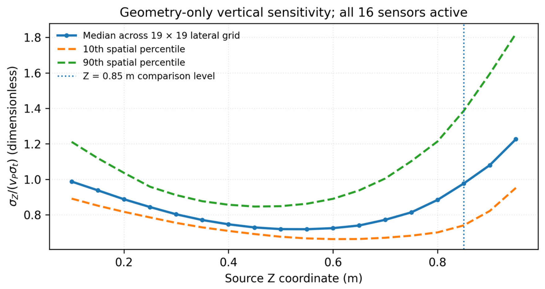
A geometry-only diagnostic uses the supplied sensor positions and the P-wave travel-time relation tj = t0 + ‖x − sj‖/vP. With origin time expressed as the distance vPt0, the Jacobian row is [ujᵀ, 1], where uj points from sensor j to the source. The positional block of (JᵀJ)⁻¹ gives dimensionless relative sensitivity under equal, independent timing errors. We report σZ/(vPσt) over 19 × 19 lateral grid positions, X,Y = 0.1–1.9 m, and Z = 0.10–0.95 m in 0.05 m increments. All 16 sensors are assumed active. No illustrative timing standard deviation is substituted for a measured localization uncertainty. The geometry-only diagnostic is distinguished from propagation of velocity-model uncertainty into event-location uncertainty [14].

Exploratory temporal analysis evaluates the fixed full-data plane in three, four and five equal-count and equal-duration windows. It does not refit a different plane in each window. A 999-permutation comparison uses the largest support range across these six partitions as one statistic per specimen. This tests time association in the retained events, not pressure-stage mechanisms. No synchronized injection-pressure record is available. Uncalibrated surface photographs are not used to tune the revision or to claim independent quantitative fracture validation; no new image calibration or blinded-rater experiment was performed.

3. Results

3.1. Revised Synthetic Reference and Information Ablations

Table 3. Revised 360-event reference family at 25% noise: mean ± SD over 20 independently generated clouds.

Scheme	Candidate ARI	Final ARI	Noise F1	Plane Recall
R	0.000 ± 0.000	0.754 ± 0.026	0.874 ± 0.023	1.000 ± 0.000
F	0.078 ± 0.026	0.787 ± 0.037	0.905 ± 0.027	1.000 ± 0.000
G	0.126 ± 0.027	0.793 ± 0.037	0.912 ± 0.026	1.000 ± 0.000
K	0.135 ± 0.036	0.797 ± 0.034	0.913 ± 0.024	1.000 ± 0.000
A	0.080 ± 0.030	0.784 ± 0.033	0.901 ± 0.027	1.000 ± 0.000
H	0.131 ± 0.043	0.295 ± 0.133	0.617 ± 0.086	0.850 ± 0.229
SR	0.598 ± 0.001	0.899 ± 0.027	0.924 ± 0.021	1.000 ± 0.000
SA	0.870 ± 0.030	0.910 ± 0.024	0.934 ± 0.017	1.000 ± 0.000
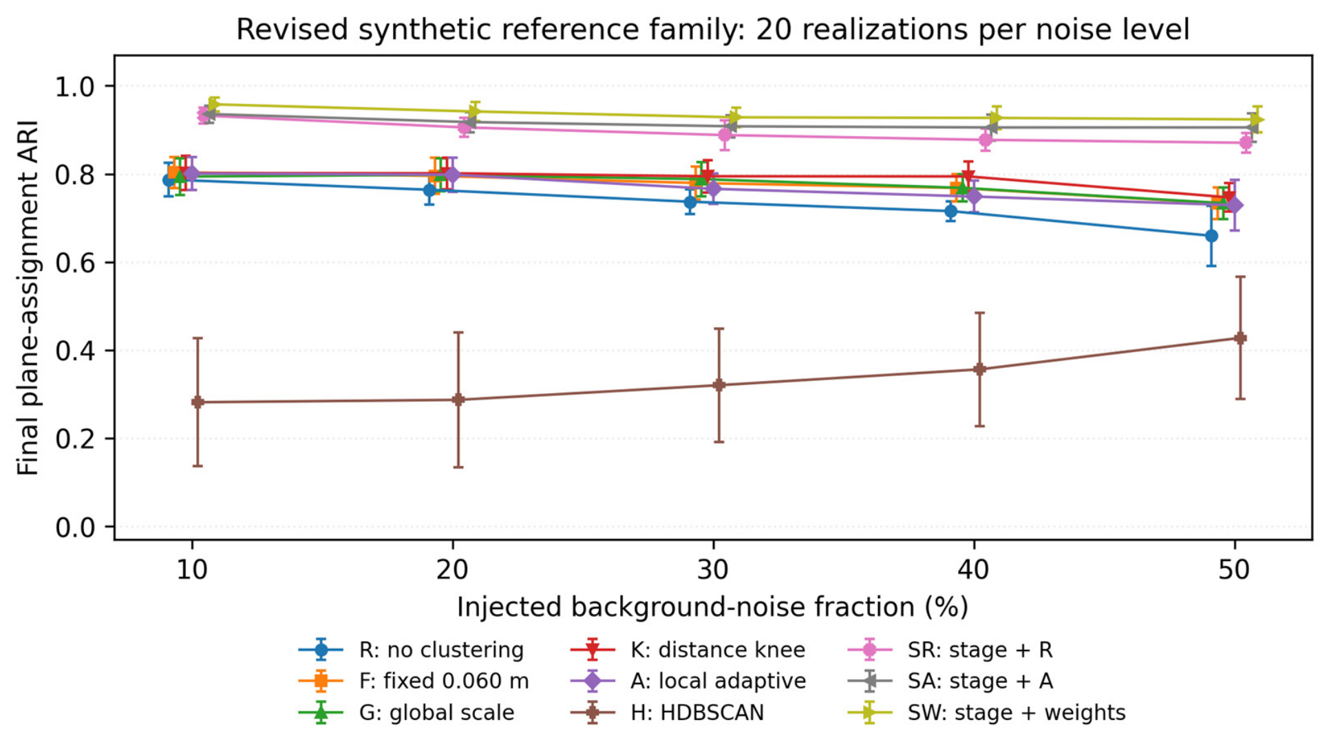
SW	0.870 ± 0.030	0.937 ± 0.020	0.952 ± 0.015	1.000 ± 0.000

reports the new 25%-noise reference family over 20 realizations. SW attained a final-assignment ARI of 0.937 ± 0.020 and noise F1 of 0.952 ± 0.015. R, F, G, K, A, SR, SA and SW recalled all three planes in every reference realization; H had a mean recall of 0.850. Thus, the original claim of a large plane-recall improvement over a single fixed-radius baseline does not carry over to this stronger comparison. A was not superior to the data-scaled fixed-radius G or K in mean final ARI. Stage information contributed substantially, as shown by SR, without requiring adaptive grouping.

Scheme definitions are in Section 2.6. Candidate ARI and final-assignment ARI describe different pipeline stages. These are new revision-stage results, not an exact replay of the lost original benchmark. Matched geometric-error statistics are given in Supplementary Table S3.

A’s candidate-group ARI was only 0.080 on average, while its final-plane ARI was 0.784. The distinction is mechanistic: spatial connectivity can unite events from different true planes, but sequential robust fitting can subsequently recover separate planar consensus sets. Candidate-group failure therefore does not imply zero plane recall. Conversely, low orientation error on the matched planes does not describe the completeness of recovery. The revised metric definitions explicitly separate these questions and prohibit geometric-error values when the eligible match set is empty. The final-assignment ARI trends over the 10–50% noise sweep are shown in Figure 2.

3.2. Failure Regimes and Conditional Benefits

The broader suite changes the interpretation from universal superiority to conditional performance. Across the five noise levels in the closely spaced parallel-plane scenario, A’s mean recall was 0.443, whereas SA and SW achieved 1.000 when correct stage labels separated the families. However, corrupting 30% of stage labels reduced the mean final ARI from 0.768 for A to 0.428 for SA and 0.439 for SW. Stages are therefore useful only when sufficiently reliable and informative; they are not declared indispensable for separating every overlapping geometry.

The smallest true plane in the 180/60/30 population scenario exposes a minimum-size failure. Mean plane recall was 0.987 for SR but 0.663 for both SA and SW: density pruning can remove an almost-threshold population before robust fitting. Unequal density also reduced SA/SW recall to 0.960 while R was 0.990 and G was 1.000. Under the specified anisotropic-error scenario, uncertainty-aware SW achieved a mean ARI of 0.931 versus 0.718 for SA, but this relies on supplied synthetic errors and cannot be asserted for the unweighted experimental runs. Curved and branched sheets degraded assignment consistency; they are retained as model-mismatch tests without a fictitious three-plane recall. Scenario summaries are in Supplementary Tables S4 and S5.

Merge sensitivity was negligible for the well-separated reference and intersecting cases, but not for the close parallel case. At a 7° angle gate and 25% noise, mean recall without stage separation was 0.733 with a 15 mm separation gate and 0.467 with either a 25 or 35 mm gate. This demonstrates that coplanar repair can merge physically distinct nearby planes. The parameters cannot be justified merely by unchanged results in a real case where only one plane is fitted.

3.3. Experimental Audit and Fair Density Baselines

Every archived subset contains 3200 unique XYZ triplets, no missing XYZ/time values and no out-of-domain or exactly boundary-clamped positions. The numbers of distinct Z values are 3137, 3124 and 3134 for S1–S3. Coordinates are serialized on a 10 μm grid, which is numerical storage precision, not measured accuracy; there is no coarse 20–40 mm storage-layer discretization that could by itself explain the observed band. Times are not sorted in file order, and file order is not assumed to preserve historical quality rank.

With the declared default parameters, A produces one candidate group containing all 3200 events in each case. Its input to the fitting kernel is consequently identical to R, and the two methods give exactly equal masks and plane parameters at the common primary seed. Adaptive connectivity is a connectivity check in these cases; it adds no event rejection or plane-separation benefit. G and K retain nearly all events and obtain comparable support. F retains only small islands, illustrating radius-transfer failure, not proving the necessity of local adaptivity. H also extracts a dominant band under its stated configuration (

Table 4. Recomputed experimental comparisons at 20 mm tolerance and primary seed 20260907.

Case	Scheme	ε (m)	Eligible Events	Support (%)	Dip (°)	RMS (mm)
S1	R	—	3200	12.38	0.97	10.96
S1	F	0.0600	106	1.25	2.52	10.28
S1	G	0.1647	3189	12.59	0.91	11.15
S1	K	0.1664	3190	12.59	0.91	11.15
S1	A	0.1647	3200	12.38	0.97	10.96
S1	H	—	1959	12.47	0.64	10.38
S2	R	—	3200	15.19	0.59	10.43
S2	F	0.0600	82	1.34	12.39	11.18
S2	G	0.1650	3194	14.81	1.02	10.35
S2	K	0.1655	3194	14.81	1.02	10.35
S2	A	0.1650	3200	15.19	0.59	10.43
S2	H	—	2061	15.00	0.45	10.25
S3	R	—	3200	11.94	1.83	11.12
S3	F	0.0600	125	2.06	15.91	12.26
S3	G	0.1639	3194	12.06	1.62	11.12
S3	K	0.1610	3188	12.78	0.44	10.86
S3	A	0.1639	3200	11.94	1.83	11.12
S3	H	—	2131	12.50	1.11	11.22

).

All schemes return one retained candidate group except F for S1, which returns two. Support is eligible inlier count divided by 3200, not all-event support retroactively recovered after excluding events. R and A are identical here. Each condition has n = 1; no injection-rate association is inferred.

The primary A/R fits contain 396, 486 and 382 events, respectively, corresponding to 12.375%, 15.1875% and 11.9375%. These replace the old unverified numerical fits. They leave 87.625%, 84.8125% and 88.0625% of the curated candidates outside the primary consensus. Those events may include vibration/background sources, distributed damage, other structures and localization error; the present data do not identify these categories individually. Enlarged event projections in Supplementary Figures S3–S5 retain all candidates rather than hiding the unassigned background.

3.4. Uniform and Marginal-Preserving Null Results

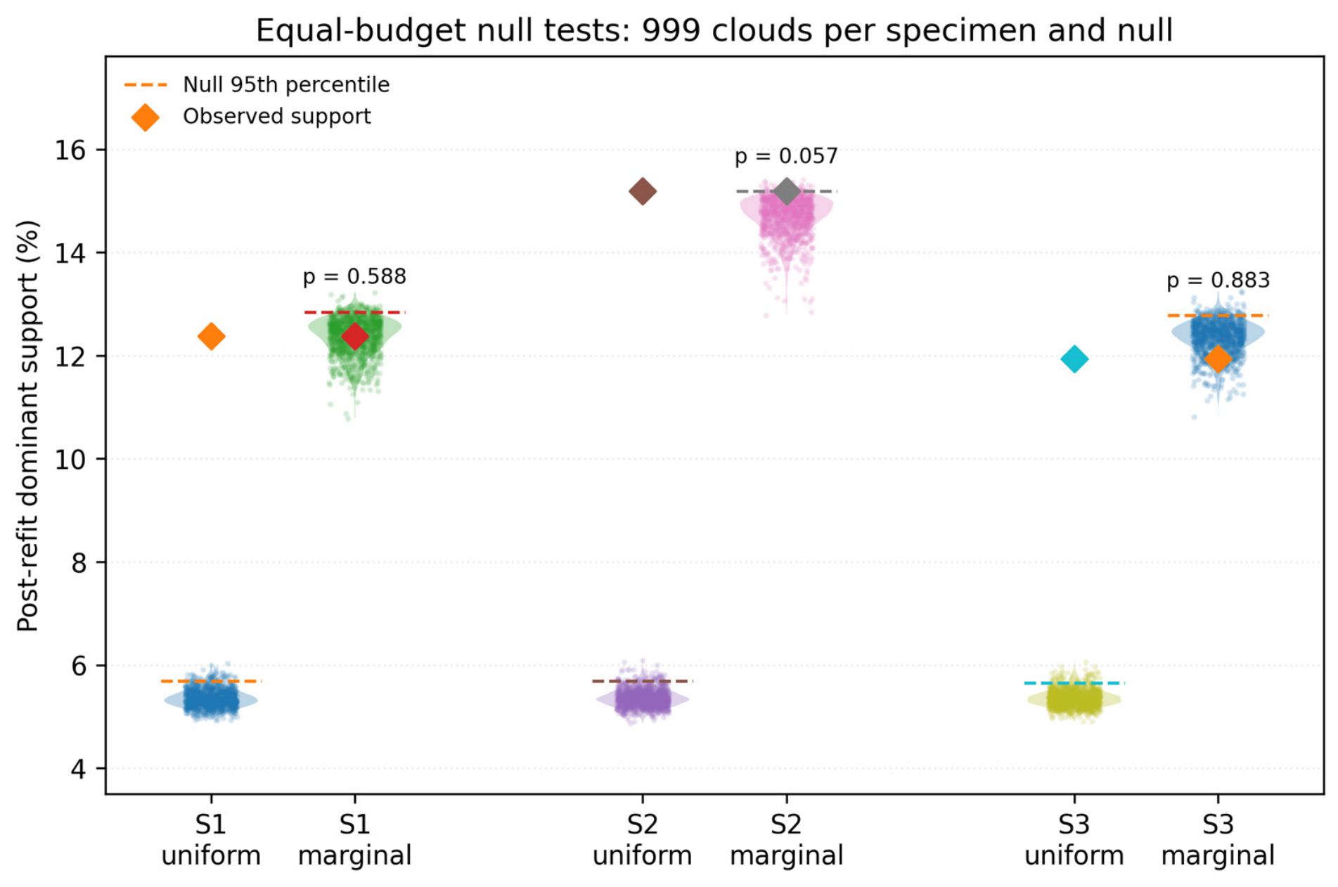
All three observed supports exceed all 999 uniform-null outcomes. Uniform-null 95th percentiles are 5.66–5.69%; their similarity is expected because volume, event count, tolerance and algorithmic budget are shared. Effect ratios relative to these percentiles are 2.18, 2.67 and 2.11. The finite p_MC values are all 0.001 at the simulation-resolution limit, with Holm-adjusted values of 0.006, rather than three precisely equal underlying tail probabilities (

Table 5. Complete-pipeline null comparisons: 999 realizations per case and null.

Case	Null	Observed (%)	Null p95 (%)	E95	p_MC	Holm p
S1	uniform	12.38	5.69	2.176	0.001	0.006
S1	marginal	12.38	12.84	0.964	0.588	1.000
S2	uniform	15.19	5.69	2.670	0.001	0.006
S2	marginal	15.19	15.19	1.000	0.057	0.171
S3	uniform	11.94	5.66	2.110	0.001	0.006
S3	marginal	11.94	12.78	0.934	0.883	1.000

).

The conclusion changes for the marginal-preserving reference. Unadjusted p_MC values are 0.588, 0.057 and 0.883 for S1–S3; none is below 0.05, and their six-test Holm-adjusted values are 1.000, 0.171 and 1.000. The observed-to-null-p95 ratios are 0.964, 1.000 and 0.934. Thus, the statistic establishes departure from spatial uniformity but not excess planar support beyond the empirical coordinate marginals. Figure 3 shows every null realization. This result is retained as a limit of the evidence, not removed in favor of the more favorable uniform reference.

Uniform-null p_MC = 0.001 is the finite Monte Carlo resolution limit (zero exceedances), not an estimate of a smaller tail probability. Marginal permutations preserve the Z concentration by design. Holm adjustment covers all six rows; no real-case fracture-detection accuracy is implied.

3.5. Sensitivity and Stability: Orientation Is Not Membership

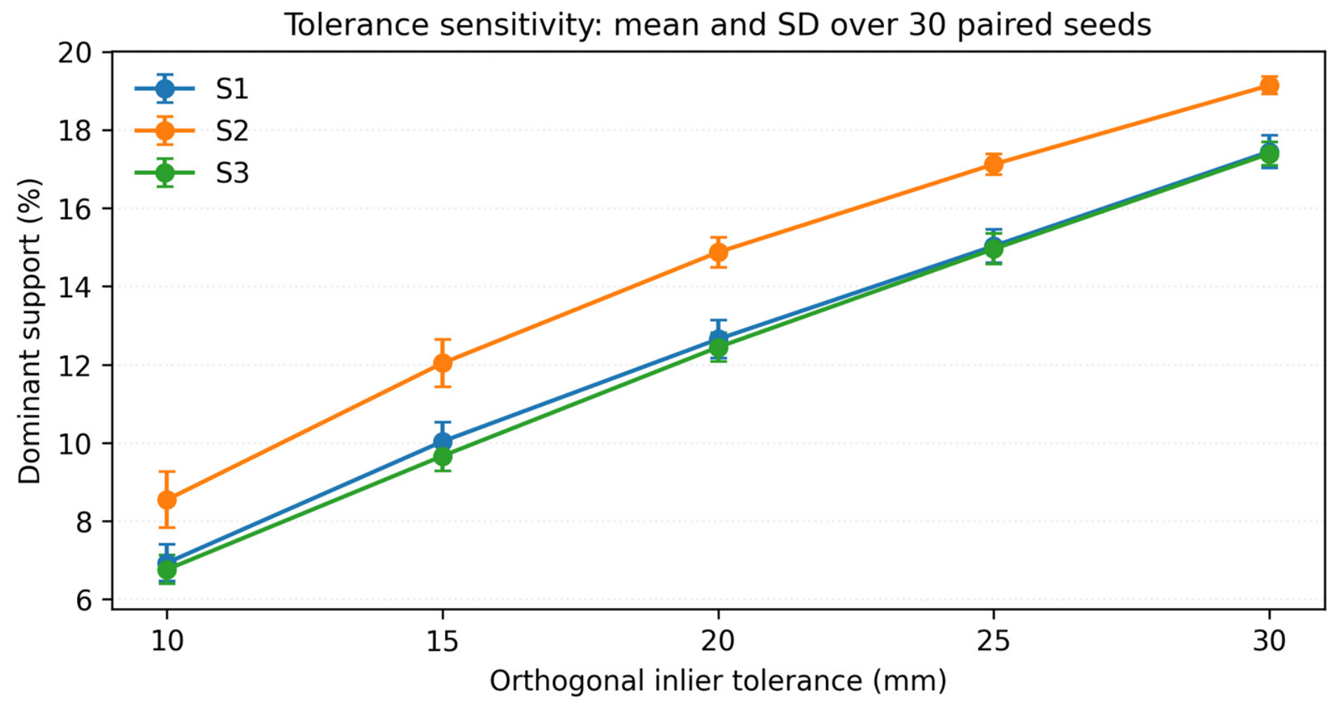
Support depends materially on the distance tolerance (Figure 4). Over 30 paired seeds, mean support increases from 6.93% to 17.44% for S1, 8.55% to 19.14% for S2, and 6.76% to 17.39% for S3 as tolerance increases from 10 to 30 mm. Mean RMS increases simultaneously from approximately 5.5–5.7 mm to 15.3–16.7 mm. Near-horizontal classification persists over the tested range, but the exact support fraction and envelope are not tolerance-invariant. Because inlier RMS is bounded by the chosen tolerance, it is not interpreted as an independently measured localization or fracture-reconstruction error.

All 39 primary connectivity perturbations per specimen retained a single candidate group, although eligible counts and random sampled triples changed when a few border points were excluded. Support ranges were 12.16–13.13%, 14.81–15.34% and 11.88–12.88% for S1–S3. These ranges characterize the stated perturbation set, not every possible setting. Global-bound perturbations are retained separately in the internal revision-stage verification package. The main conclusion—that a single connected group is passed to robust fitting—does not depend on the default local-radius formula alone.

All 200 80%-subsample runs recovered a plane for each case. Membership-and-geometry matches numbered 194/200, 200/200 and 107/200, respectively (

Table 6. Conditional stability relative to the primary full-data plane.

Case	80% Match Rate	Full-Data Seed Matches	Normal Difference (°)	Support (%)	Envelope Area (m2)
S1	194/200 (97.0%)	192/200	0.20–1.92	11.80–13.52	3.54–3.74
S2	200/200 (100.0%)	199/200	0.12–1.11	13.87–15.78	3.59–3.75
S3	107/200 (53.5%)	93/200	0.27–2.69	11.48–13.28	3.58–3.77

). S3 therefore has only a 53.5% match rate despite a narrow range of normal-angle differences. Its full-data 200-seed match rate was similarly low, 93/200, compared with 192/200 and 199/200 for S1 and S2. This identifies substantial random-search/membership variation in a broad near-horizontal concentration, not simply event-deletion uncertainty. All distributions include non-matching fits; reporting only matched orientations would conceal this behavior.

Intervals are empirical 2.5th–97.5th percentiles over all recovered 80%-subsample fits, not physical-fracture confidence intervals. A match requires ≤5° normal difference, ≤40 mm height offset at the specimen center, and ≥0.50 full-table Jaccard overlap. All fits, including non-matches, remain in the reported distributions.

3.6. Geometric Descriptors and the Repeated Z Concentration

The primary planes are nearly horizontal, with dips of 0.974°, 0.590° and 1.828°. Heights at the wellbore axis are 0.8302, 0.8518 and 0.8514 m. Plane equations, normals, centers, projected dimensions, convex-envelope areas and predicted specimen-boundary intersections are provided in Supplementary Table S6 and retained in the internal revision-stage verification package. Strike is explicitly specimen-referenced and poorly conditioned for a nearly horizontal plane; it is not presented as a geographic fracture azimuth.

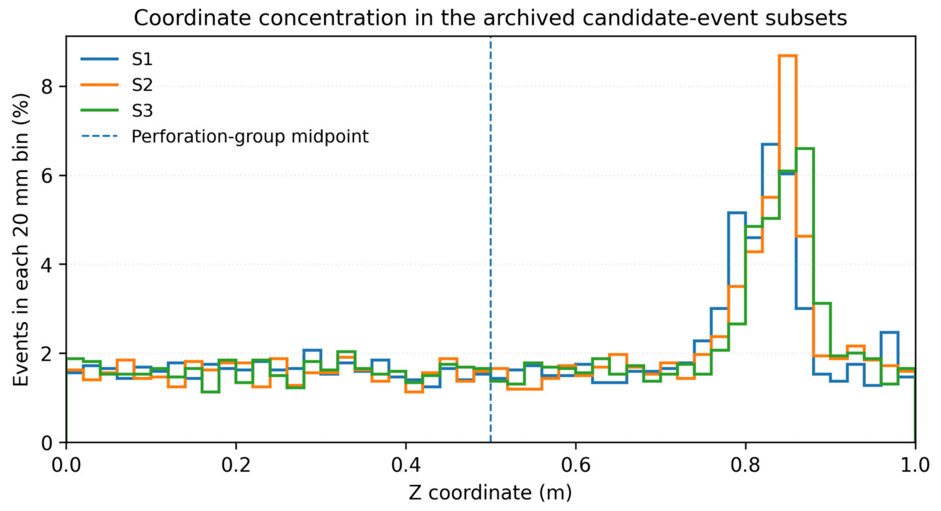
Figure 5 confirms that the Z marginal already contains a strong upper-specimen concentration. The fitted wellbore-axis heights lie approximately 0.33–0.35 m above the perforation-group midpoint at Z = 0.50 m. Alignment of a plane normal with the least-loaded Z axis is mechanically compatible with the loading convention but does not independently explain this height offset or establish the source mechanism. A material interface, boundary-associated response, non-fracture vibration, selection effects, velocity-model error and other localization biases cannot be separated using the available records.

The geometry-only vertical sensitivity has a lateral-grid median of 0.719 at Z = 0.50 m and 0.976 at Z = 0.85 m (Figure 6). Thus, the upper band is not explained by that layer having the smallest median vertical sensitivity under the assumed all-sensor, equal-timing-error model. This is a restricted diagnostic, not exclusion of array-induced bias. Actual event-wise channel participation, correlated pick errors, velocity heterogeneity and calibration shots are unavailable; the Jacobian model neither recreates historical locations nor supplies empirical accuracy bounds.

3.7. Exploratory Temporal Association

Fixed-plane membership is associated with event time under equal-count and equal-duration partitions. The maximum window-support range across the six partitions was 0.269, 0.341 and 0.234 for S1–S3, exceeding all 999 temporal permutations in each case. This result concerns only the curated event-time pairing. It neither identifies pressure stages nor establishes initiation, propagation or shut-in mechanisms. Detailed window counts and fractions are retained in Supplementary Table S7 and in the internal revision-stage verification package rather than used to make a central engineering conclusion.

4. Discussion

4.1. What the Integrated Workflow Contributes

The comparisons isolate three effects that the original single-baseline argument conflated. Selecting a workable global density scale prevents fragmentation by an underscaled radius. Local-radius adaptation is a separate option and did not outperform all data-scaled alternatives in the new reference suite. Robust fitting can recover a dominant plane even when candidate clustering supplies no partition. For the experimental subsets, the no-clustering and adaptive runs are exactly equal at the declared primary setting. This is direct evidence of limited added value from clustering in these cases, not a reason to attribute the full result to DBSCAN.

The optional stage and uncertainty modules have information-dependent value. Correct stage labels can separate nearby families that spatial density alone merges, but the stage-raw control shows that much of this gain comes from the labels themselves. Incorrect labels or pruning of small populations can reverse the advantage. A weighted method additionally assumes useful error information; the synthetic demonstration is conditional on its supplied error model. The contribution relative to established density-constrained and multi-model fracture methods [2,6] is therefore the auditable integration and the explicit separation of these effects, rather than an unqualified claim to a novel or fully automatic fracture-reconstruction principle.

4.2. What the Experimental Planes Do and Do Not Establish

The experimental outputs are geometric summaries of quality-selected event-location subsets. They do not identify the full acoustic-emission catalog, the number of true fracture sources, stimulated reservoir volume, opened area, conductive area or propped area. Convex-envelope areas are especially easy to overinterpret because dispersed coplanar inliers can span most of the specimen face; the envelope fills unobserved gaps. Boundary intersections are predictions from the fitted infinite plane and the specimen box, not measured surface traces. Reservoir-scale work likewise treats stimulated extent and fracture conductivity as distinct descriptors of stimulation performance [26].

Wang et al. used a coupled three-dimensional model to examine how bedding and stress combinations control vertical hydraulic-fracture propagation [27]. Together with the laboratory observations of interface interaction and fracture branching [3,4], this provides a physical reason not to equate one planar consensus with a complete fracture trajectory. The present algorithm does not simulate those coupled propagation processes or establish bedding-controlled growth in S1–S3.

Recent large-scale fracturing studies further support this separation between monitoring-derived geometry and the complete physical fracture system. A three-meter-scale reconstituted tight-conglomerate study combined acoustic-emission locations with DBSCAN-based filtering and geometric reconstruction, demonstrating the feasibility of event-cloud interpretation over meter-scale propagation distances [28]. In a 2 m × 2 m × 1 m sand-conglomerate block, distributed fiber-optic monitoring linked high-frequency acoustic-emission activity and low-frequency strain responses to fracture evolution, while still requiring independent mechanical interpretation of the monitored signals [29]. Complementary 20 m rough-wall experiments and Fluent/CFD-DEM screening studies show that proppant placement depends strongly on fracture roughness, flow conditions and particle transport dynamics [30,31]. Together, these studies reinforce that a dominant microseismic event plane should be treated as one observational layer rather than as a direct measurement of opened, conductive or propped fracture area.

The two null models make the interpretation boundary quantitative. Uniform-cloud rejection says that these subsets are not adequately described as uniform random locations at the imposed tolerance. Non-rejection of the marginal-preserving references says that dominant support does not establish additional structure beyond their observed coordinate distributions. The retained Z concentration may have a physical origin, a processing origin or a mixture; the test does not decide among them. Similarly, stable dip classification does not guarantee stable membership, as S3 demonstrates. These limitations should remain adjacent to the numerical results rather than be confined to a final disclaimer.

Injection rate is recorded as an experimental condition only. There is one specimen per rate, no retained pressure synchronization and no independently measured fracture-surface ground truth. Ranking three support values, whether monotonic or not, cannot separate rate response from specimen variation, candidate selection and search variability. The revision therefore removes rate-effect language and uncalibrated-photograph validation claims from the abstract and conclusions.

4.3. Reproducibility and Unresolved Limitations

The internal revision-stage verification package records inputs, hashes, exact generators, realized synthetic truth, parameters, software versions, random seeds, all simulation outcomes and tests of numerical consistency. It supports verification of the revision-stage calculations and may be provided in selected form to journal editors or reviewers upon reasonable request, subject to project authorization. It does not recover the original benchmark or make the preceding experimental selection independently reproducible. The historical quality indicators and their combined ranking rule are absent, so the representativeness of the retained 3200 points remains unquantified. Random subsampling within them cannot repair this missing information.

The synthetic suite is broader than a single idealized example but is not an exhaustive physical model. It uses simplified planar patches, Gaussian localization perturbations, prescribed background processes and particularly favorable stage labels in some scenarios. The curved/branched tests reveal limits rather than demonstrate nonplanar recovery. HDBSCAN and fixed-radius competitors are evaluated under stated operational choices, not every possible tuning strategy. The normal-angle and center matching gates are operational benchmark definitions, not universal geological tolerances.

No empirical localization calibration, raw-waveform reprocessing, quantitative surface registration, CT comparison, sectioning validation or blinded image-rater study has been added. Removing such claims is not equivalent to obtaining the missing validation. Future physical verification requires traceable complete event exports with picks, channel masks and quality fields, an independently specified selection rule, synchronized injection records, and calibrated post-fracturing geometry. Until then, the experimental evidence supports conditional event-plane extraction and diagnostic assessment only.

5. Conclusions

• A revision-stage, reproducible implementation specifies adaptive connectivity, support-first plane fitting, optional stage/error information and coplanar repair, while making parameter provenance and missing historical records explicit. It is not presented as a parameter-free reconstruction of hydraulic-fracture surfaces.
• Across a new 1120-cloud synthetic suite, correct stage information and supplied uncertainty can improve assignment quality, but wrong stages, small populations, nearby planes and nonplanar surfaces expose important failures. At 25% reference noise, SW achieved ARI 0.937 ± 0.020 and noise F1 0.952 ± 0.015; these are synthetic results, not experimental detection accuracies.
• In all three curated 3200-event subsets, default adaptive connectivity retained every event as one group. The resulting primary planes were identical to direct RANSAC, with 11.94–15.19% support. Data-scaled fixed-radius and HDBSCAN comparisons do not support a blanket experimental superiority claim for local adaptivity.
• Equal-budget null tests reject a uniform-cloud reference but not coordinate-marginal-preserving references. Support and RMS depend on tolerance, and S3 has only 53.5% reference-membership matches under 80% subsampling despite near-horizontal orientation stability. The physically opened fracture, its area and injection-rate dependence remain unvalidated.