A Reliable Defect Confirmation Method for Drainage Pipeline Inspection Based on Vision–LiDAR–Ultrasonic Fusion

Abstract

Drainage pipeline environments are typically characterized by darkness, high humidity, water accumulation, sediment deposition, reflective surfaces, and severe occlusions. These challenging conditions make conventional single-sensor inspection methods highly susceptible to environmental interference, resulting in false detections, missed defects, and insufficient reliability in defect confirmation. To address these challenges, this paper proposes a vision–LiDAR–ultrasonic multi-sensor fusion method for defect confirmation in drainage pipeline inspection. The three sensing streams are processed in parallel rather than using visual detection as the exclusive trigger: the vision branch performs high-recall screening of apparent defects, the LiDAR branch continuously evaluates geometric anomalies in spatially indexed point-cloud segments, and the ultrasonic branch independently evaluates wall-thickness and echo anomalies along the valid probe-contact path. Candidate regions proposed by any branch are merged through timestamp-, odometry-, and coverage-aware spatial association, after which all available visual, geometric, and acoustic evidence at each union candidate is mapped to basic probability assignments and fused using reliability-constrained Dempster–Shafer evidence theory. The five-run evaluation on the fixed 105-group test subset (18 defects and 87 non-defects) gives the proposed method an Accuracy of 97.7 ± 0.5%, Precision of 93.4 ± 2.2%, Recall of 93.3 ± 2.5%, F1-score of 93.3 ± 1.5%, and false-alarm rate of 1.4 ± 0.5%. Under the same test protocol, the vision-only baseline gives an F1-score of 81.1 ± 2.4% and a false-alarm rate of 3.9 ± 0.6%. These results are calculated from the measured per-group predictions obtained in the experiments.

1. Introduction

Urban drainage pipelines are critical underground infrastructure for urban flood control, stormwater drainage, water environment management, and public safety. With the continuous expansion of urban built-up areas and the increasing service life of underground pipeline networks, drainage pipelines are becoming increasingly susceptible to various types of structural defects, including aging, joint misalignment, cracks, corrosion, leakage, and sediment blockage [1,2,3]. If these defects cannot be detected and accurately confirmed in a timely manner, they may lead to road collapse, sewage leakage, stormwater–sewage cross-connections, urban flooding, and reduced operational efficiency of drainage networks, thereby posing significant risks to urban safety and refined infrastructure management [4,5,6]. Therefore, achieving highly reliable defect detection and confirmation in complex pipeline environments has become a critical research issue in the intelligent inspection and maintenance decision-making of urban drainage pipeline networks.

Conventional drainage pipeline inspection mainly relies on closed-circuit television (CCTV), manual interpretation, and experience-based assessment. Owing to its mature equipment, ease of operation, and intuitive inspection results, CCTV remains one of the most widely adopted techniques for drainage pipeline inspection [4,7]. 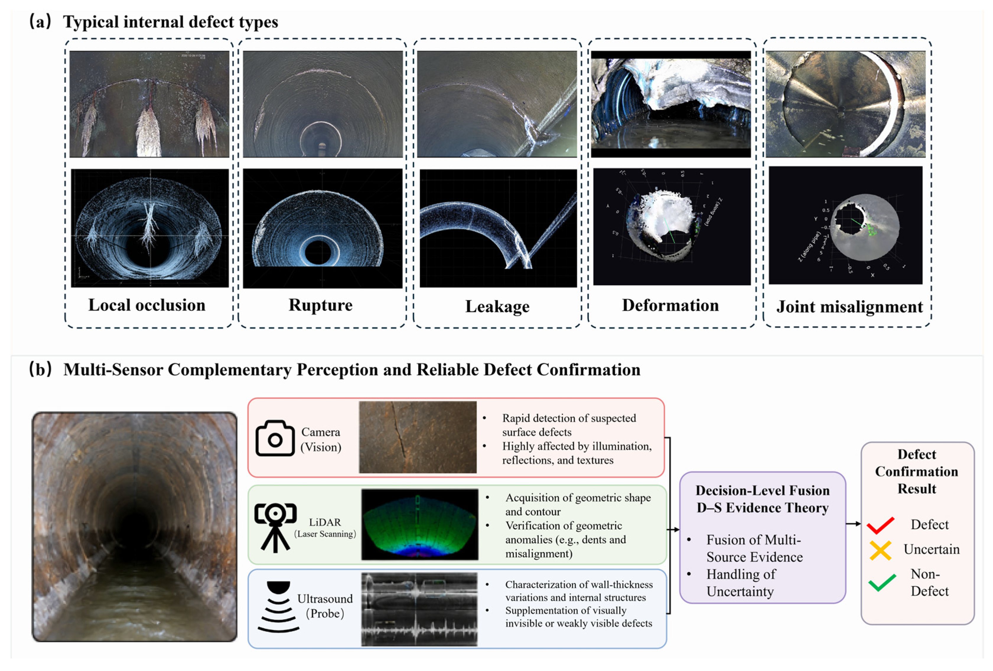However, drainage pipelines are typically characterized by challenging environmental conditions, such as darkness, high humidity, standing water, sediment accumulation, reflective surfaces, fog, occlusions, and confined spaces, which often result in unstable image quality and make manual interpretation susceptible to subjective judgment and differences in inspector experience [5,8]. Moreover, visual images primarily provide information on the pipe surface and have limited capability in confirming defects such as wall-thickness reduction, internal voids, submerged defects, and slight geometric deformations. Consequently, the results obtained from a single vision-based inspection are often insufficient to serve as a reliable basis for maintenance decision-making. These representative inspection challenges and defect manifestations are summarized in Figure 1. The examples shown in Figure 1a are intended to illustrate typical field conditions and observable abnormal phenomena rather than to provide an exhaustive list of the defect categories evaluated in this study. The quantitative experiments in this study focus on cracks, corrosion/spalling, joint misalignment, and wall-thickness reduction, as detailed in Section 3.2. As illustrated in Figure 1b, the three sensing modalities provide complementary information for defect confirmation: vision captures surface appearance, LiDAR characterizes geometric anomalies, and ultrasonic sensing provides information on wall-thickness variation and internal damage.

In recent years, deep learning techniques have been widely introduced into automated defect detection for drainage pipelines. Convolutional neural networks (CNNs), Faster R-CNN, the YOLO series, U-Net, and Transformer-based models have been extensively applied to defect classification, object detection, and semantic segmentation of pipeline images [9,10,11,12,13,14,15,16,17]. Existing studies have demonstrated that deep learning models can automatically learn representative features of defects, such as cracks, corrosion, structural damage, tree root intrusion, and joint anomalies, from CCTV images, thereby improving inspection efficiency and reducing the workload associated with manual interpretation [10,11,12,13,14]. For example, large-scale public datasets such as Sewer-ML have significantly promoted research on image-based pipeline defect classification [8], while methods based on Faster R-CNN, YOLO, and improved convolutional networks have further enhanced defect localization accuracy and real-time detection performance [10,15,16,17,18]. Furthermore, to address challenges such as class imbalance, multi-label defect coexistence, and complex background interference, researchers have introduced techniques including multi-task learning, label correlation modeling, attention mechanisms, and uncertainty estimation, thereby improving the robustness and recognition performance of deep learning models in complex inspection scenarios [19,20,21,22,23].

Despite the rapid development of vision-based intelligent inspection methods, existing studies still exhibit three major limitations. First, most methods primarily focus on whether a defect can be detected, while insufficient attention has been paid to the reliability of the detection results. In practical engineering applications, the bounding boxes or segmented regions produced by vision models do not necessarily correspond to confirmed defects. In particular, under challenging conditions such as uneven illumination, water-surface reflections, surface contamination, and complex pipe-wall textures, vision models are prone to falsely identifying non-structural textures as defects [7,21]. Second, visual images are inherently limited in representing geometric deformations and internal structural damage. Consequently, visual evidence alone is often insufficient for confirming defects such as joint misalignment, local deformation, wall-thickness reduction, and submerged defects [4,5]. Third, although some deep learning models have achieved promising performance on benchmark datasets, they still suffer from limited generalization when applied across different pipe diameters, materials, water levels, and urban environments [17,22]. Therefore, intelligent inspection of drainage pipeline defects should not rely solely on vision-based detection but should further incorporate a multi-source information fusion mechanism for reliable defect confirmation in practical engineering applications.

Beyond vision-based inspection, non-visual sensing technologies, including LiDAR, three-dimensional point clouds, sonar, and ultrasonic testing, have gradually been applied to underground pipeline inspection and condition assessment [24,25,26,27,28,29,30,31]. Among these techniques, LiDAR and laser profile scanning can capture the internal geometric profiles of pipelines, providing effective characterization of geometric anomalies such as pipe-wall deformation, joint misalignment, sediment accumulation height, and local depressions [24,25,30]. Ultrasonic inspection can evaluate variations in pipe-wall thickness, material defects, and internal damage based on echo time, amplitude, and spectral characteristics, demonstrating advantages in confirming invisible or weakly visible defects that are difficult to identify through visual sensing alone [27,28]. However, LiDAR-based sensing has limitations in detecting underwater regions and highly absorptive media, while ultrasonic inspection is often affected by coupling conditions, inspection efficiency, and sensor deployment configurations, making it difficult to achieve comprehensive and efficient full-range inspection independently. Therefore, different sensing modalities should not be considered as simple substitutes for each other; instead, they exhibit strong complementary characteristics and can provide mutually beneficial information for reliable pipeline defect assessment.

Although dual-sensor combinations can partially compensate for the limitations of a single sensing modality, they still cannot provide complete complementary evidence for all defect types considered in drainage pipeline inspection. For example, vision–LiDAR fusion can combine surface appearance with geometric information, but it remains limited in confirming wall-thickness reduction and internal damage that may not produce obvious visual or geometric responses. Conversely, vision–ultrasonic fusion can provide surface and acoustic evidence, but it lacks the direct three-dimensional geometric characterization required for defects such as pipe deformation and joint misalignment. Therefore, the simultaneous use of vision, LiDAR, and ultrasonic sensing provides complementary surface, geometric, and internal structural information, which is particularly important for reliable confirmation of heterogeneous pipeline defects.

Multi-sensor fusion provides a feasible approach to improving the reliability of defect confirmation in drainage pipeline inspection. Visual images enable rapid screening of apparent surface defects, LiDAR point clouds provide independent geometric evidence, and ultrasonic signals provide independent acoustic information on wall-thickness variations and internal damage within their effective sensing coverage [24,25,26,27,28,29,30,31]. Importantly, a multi-sensor confirmation system should not require one modality to generate a candidate before the other modalities are allowed to contribute; otherwise, a defect invisible to the triggering modality may never reach the fusion stage. Dempster–Shafer (D–S) evidence theory is capable of handling uncertain information and combining evidence from multiple sources and has therefore been widely applied to fault diagnosis, target recognition, and multi-sensor decision fusion [32,33,34,35,36]. Compared with simple weighted averaging, D–S evidence theory can explicitly represent the states of “defect,” “non-defect,” and “uncertainty,” thereby providing an interpretable fusion framework for defect confirmation in complex environments. Therefore, the key issue addressed in this study is not only cross-modal verification of visually detected regions, but also sensor-independent candidate generation followed by consistent cross-modal association and confirmation.

Based on the above analysis, this paper proposes a vision–LiDAR–ultrasonic fusion method for reliable defect confirmation in drainage pipeline inspection. The visual detector is retained as a high-throughput candidate generator for apparent defects, but it is no longer the exclusive entrance to the confirmation pipeline. LiDAR and ultrasonic streams are also analyzed independently to identify geometric and acoustic anomalies within their valid sensing coverage. The candidate sets generated by the three branches are merged, and the corresponding visual image, local point cloud, and ultrasonic echo are associated at each candidate location. Finally, a decision-level fusion mechanism based on Dempster–Shafer (D–S) evidence theory is used to generate the final defect confirmation confidence. The main contributions of this study are summarized as follows:

(1)

A sensor-independent candidate-generation and decision-level fusion framework integrating vision, LiDAR, and ultrasonic sensing is proposed for complex drainage pipeline environments. Visual, geometric, and acoustic anomaly branches operate in parallel, and a candidate proposed by any valid sensing branch can enter the subsequent cross-modal confirmation stage.

(2)

A common spatial association and modality-specific evidence representation scheme is established without requiring a provisional defect class. Candidate regions from the visual, LiDAR, and ultrasonic branches are transformed into a shared pipe-centered coordinate, merged using timestamp, odometry, and physical-coverage constraints, and represented by modality-level anomaly scores at the same physical location. Defect-type labels are used only for descriptive subgroup analysis and are not required by the proposed binary D–S confirmation rule.

(3)

Dempster–Shafer (D–S) evidence theory is introduced to fuse confidence information from multiple sensing modalities. The visual detection confidence, degree of geometric anomaly derived from point clouds, and ultrasonic echo responses are uniformly mapped into multi-source evidence, thereby improving the interpretability and reliability of defect confirmation under complex environmental conditions.

(4)

The engineering applicability of the proposed method is validated through field experiments conducted in drainage pipelines. Comparative evaluations are performed against vision-only, LiDAR-only, ultrasonic-only, and simple fusion strategies to quantify the contribution of each sensing modality to defect confirmation performance.

2. Method

2.1. Overall Framework

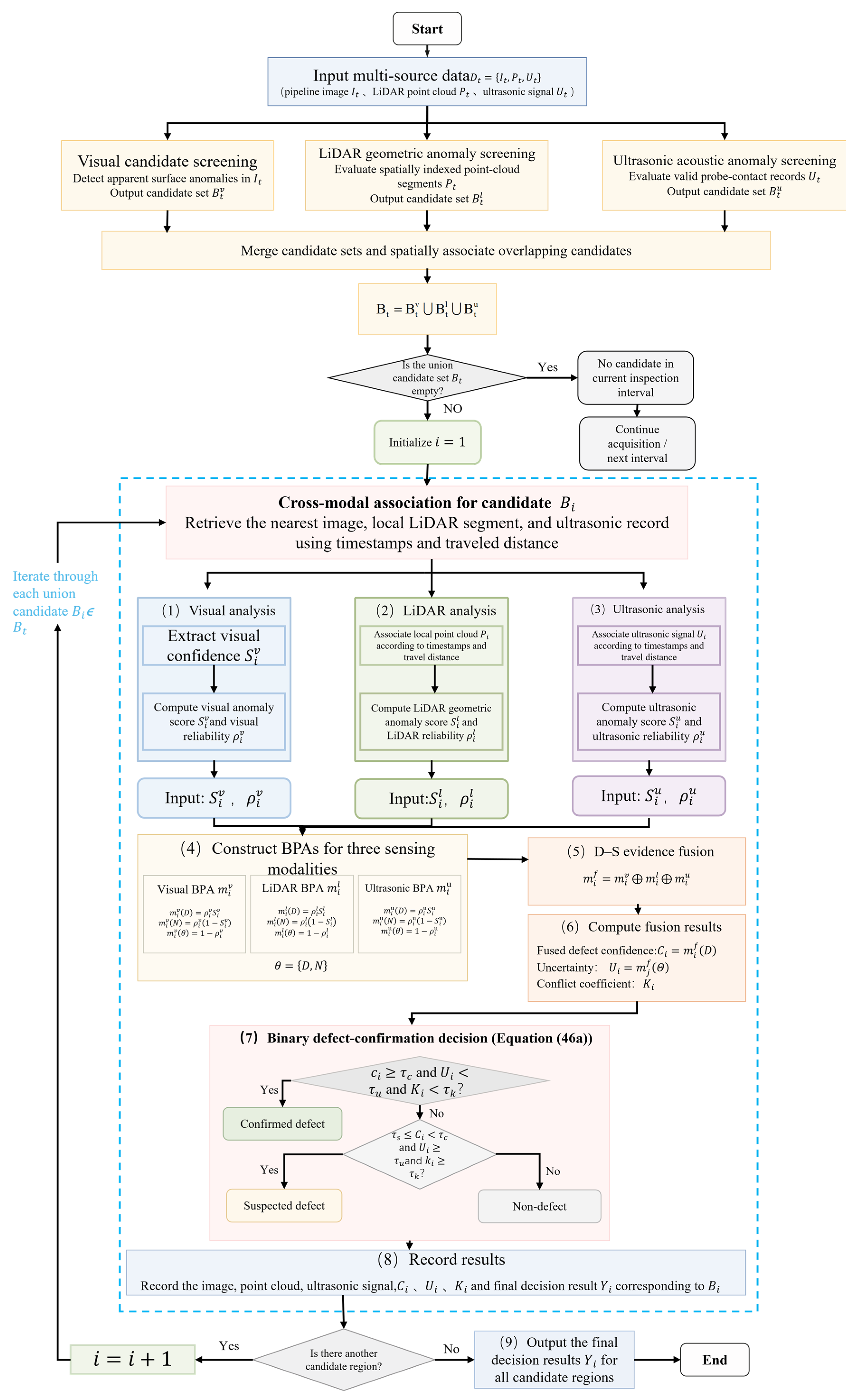
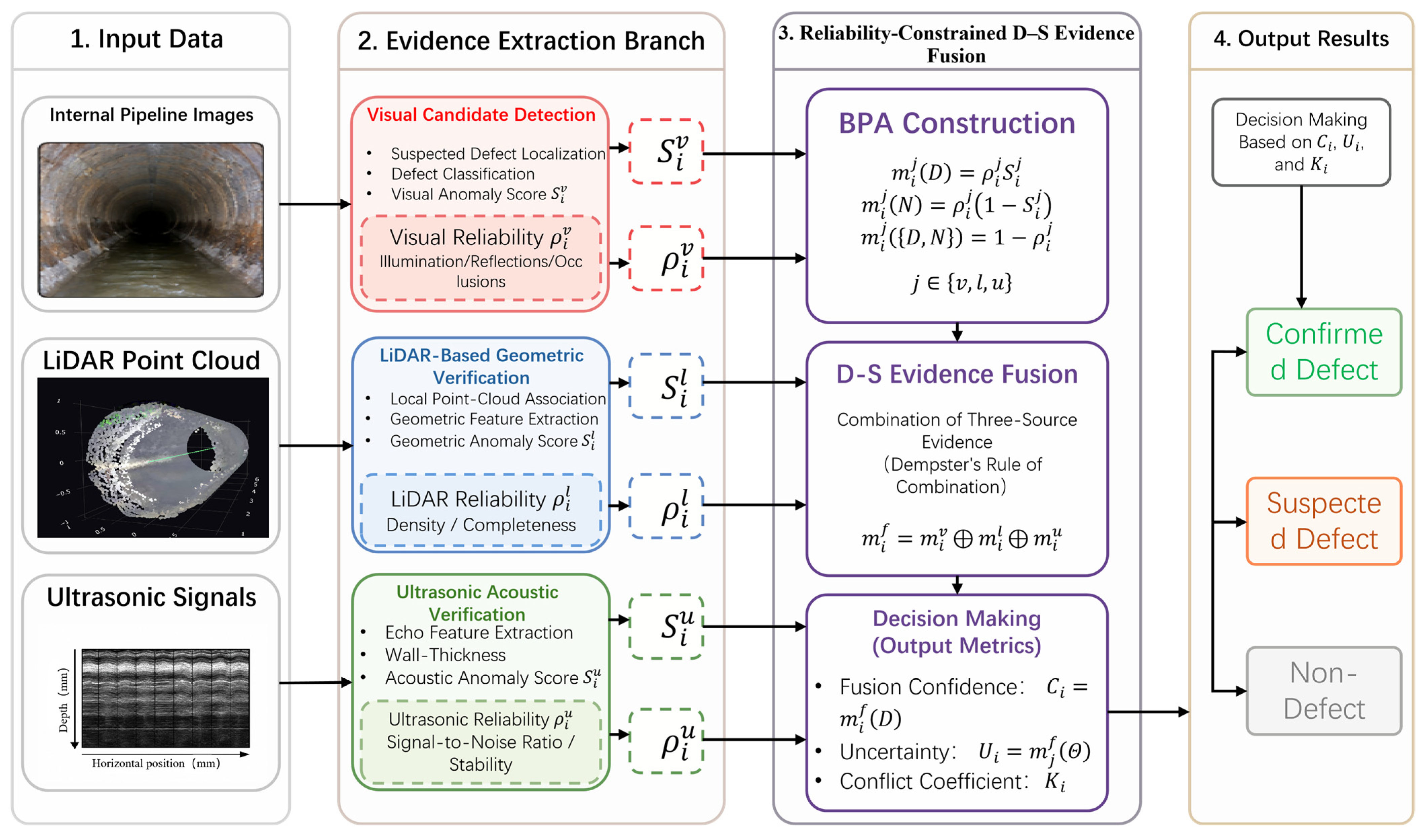
Drainage pipeline interiors are typically characterized by low illumination, standing water, sediment accumulation, reflective surfaces, fog, and partial occlusions, which make single-sensor inspection methods prone to false detections and missed detections in practical applications. To address this issue, this paper proposes a vision–LiDAR–ultrasonic fusion method for reliable defect confirmation in drainage pipelines. The proposed method adopts a “parallel screening–association–confirmation” process: each sensing modality first evaluates its own data stream, candidate regions proposed by any branch are spatially associated, and reliability-constrained multi-source evidence fusion is then used to determine whether the associated region corresponds to an actual defect.

The overall workflow of the proposed method is illustrated in Figure 2. At the acquisition layer, the camera, LiDAR, and ultrasonic channels operate continuously during robot motion, and their measurements are timestamped and indexed by traveled distance. At the processing layer, the three synchronized streams are screened independently rather than using the visual result as a prerequisite for the other sensing modalities. The vision branch performs high-recall screening of surface-visible defects, the LiDAR branch evaluates spatially indexed point-cloud segments for geometric anomalies, and the ultrasonic branch evaluates valid probe-contact positions for wall-thickness and echo anomalies. The candidate sets generated by the three branches are merged into a union candidate set. Therefore, a LiDAR or ultrasonic anomaly remains eligible for confirmation even when no visual bounding box is produced at the same location. For each union candidate, the corresponding image, local point-cloud segment, and ultrasonic record are retrieved using acquisition time and robot travel distance, and the resulting visual, geometric, and acoustic evidence is subsequently fused using reliability-constrained Dempster–Shafer evidence theory.

Compared with conventional vision-only inspection methods, the innovations of the proposed method are mainly reflected in the following three aspects. First, a “parallel screening–association–confirmation” procedure is proposed for pipeline defect assessment. Simultaneous multi-sensor acquisition is separated conceptually from candidate generation: each sensing modality can independently nominate an anomalous location within its effective coverage, and only the union of these candidates is passed to cross-modal confirmation. Thus, visual detections are one source of candidates rather than a mandatory gate for LiDAR and ultrasonic analysis. Second, a class-independent, modality-specific evidence representation is established in a common physical coordinate. Vision describes surface appearance, LiDAR describes geometric/continuity abnormalities, and ultrasonic sensing describes wall-thickness and acoustic abnormalities; these three modality scores are constructed before fusion without assuming whether the candidate is a crack, corrosion/spalling, joint misalignment, or wall-thinning case. Third, a reliability-constrained Dempster–Shafer evidence fusion mechanism is developed. Sensor reliability coefficients based on image quality, point-cloud completeness, and ultrasonic signal quality are incorporated into the basic probability assignments so that the final binary confirmation reflects both evidence strength and the current reliability of each sensing modality.

2.2. Multi-Sensor Data Acquisition and Sensor-Independent Candidate Association

The inspection system consists of a vision camera, a LiDAR sensor, an ultrasonic probe, and an embedded computing unit. The multi-source data acquired by the inspection robot at time t are expressed as:

$$D_t=\left\{I_t,\hspace{0.33em}{P}_t,\hspace{0.33em}{U}_t\right\}$$

(1)

where $I_t$ denotes the image of the pipeline interior, $P_t=\{p_k{\}}_{k=1}^M$ denotes the LiDAR point cloud, $p_k=\left(x_k,y_k,z_k\right)$ represents the three-dimensional coordinates of the $k$-th point, and denotes the ultrasonic time-domain echo signal $U_t=\left\{u\left(\tau \right)\right\}$.

Because the vision camera, LiDAR sensor, and ultrasonic probe operate at different sampling frequencies and are mounted at different positions on the robot, cross-modal association is performed in a common robot-centered coordinate rather than by comparing acquisition indices directly. For a record i from modality a and a candidate record j from modality b, the actual acquisition timestamps and encoder-derived axial coordinates are used after compensating for the calibrated sensor mounting offsets. The associated record is selected by the normalized temporal–spatial distance in Equation (2a):

$$j^{\ast }=\mathrm{a}\mathrm{r}\mathrm{g}\underset{j}{\mathrm{m}\mathrm{i}\mathrm{n}}\left[{\lambda }_t{\displaystyle \frac{\left|t_i^a-t_j^b\right|}{\Delta t_{\mathrm{m}\mathrm{a}\mathrm{x}}}}+{\lambda }_s{\displaystyle \frac{\left|\left(s_i^a+{\delta }_a\right)-\left(s_j^b+{\delta }_b\right)\right|}{\Delta s_{\mathrm{m}\mathrm{a}\mathrm{x}}}}\right], a,b\in \left\{v,l,u\right\},\hspace{0.25em}a\ne b$$

(2a)

where denote the timestamp and encoder-derived axial coordinate $t_i^a \mathrm{a}\mathrm{n}\mathrm{d} s_i^a$ of record i from modality a, ${\delta }_a$ denotes the calibrated axial mounting offset of that sensor relative to the robot reference point, and ${\lambda }_t$ and ${\lambda }_s$ are non-negative association weights satisfying ${\lambda }_t + {\lambda }_s = 1$. Associations are accepted only when the absolute inter-sensor timestamp difference is within the 50 ms tolerance used in the experiments and the axial separation is within the calibrated spatial association window. The same rule is applied symmetrically regardless of which sensing branch initiates the candidate.

Because the contact-ultrasonic probe observes only the pipe-wall strip physically intersected by its contact path, axial proximity alone is not sufficient to declare ultrasonic evidence available. Each union candidate is represented by an axial coordinate $s$ and a circumferential coordinate $\theta$. Circumferential separation is measured with the periodic angular distance below and converted to arc length using the local pipe radius $R_i$. Ultrasonic evidence is available only when Equation (2b) is satisfied:

$$\begin{gathered} M_i^u=\mathbf{1}\left(\left|s_i-s_i^u\right|\le \Delta s_u\hspace{0.25em}\wedge \hspace{0.25em}{R}_i{d}_{\theta }\left({\theta }_i,{\theta }_i^u\right)\le \Delta {\mathcal{l}}_u\right) \\ d_{\theta }\left({\theta }_1,{\theta }_2\right)=\mathrm{m}\mathrm{i}\mathrm{n}\left(\left|{\theta }_1-{\theta }_2\right|,\hspace{0.25em}2\pi -\left|{\theta }_1-{\theta }_2\right|\right) \end{gathered}$$

(2b)

Here, $M_i^u$ is the ultrasonic-coverage indicator, ${\Delta s}_u$ is the axial half-window, and ${\Delta \mathcal{l}}_u$ is the circumferential arc-length half-window of the usable probe footprint after calibration. In the present experimental configuration, ${\Delta s}_u = 15 \mathrm{m}\mathrm{m}$ and ${\Delta \mathcal{l}}_u = 10 \mathrm{m}\mathrm{m}$ are the calibrated coverage settings used in the experiments, determined from the probe footprint and synchronization tolerance. When $M_i^u = 0$, the ultrasonic modality is unavailable at that candidate and its reliability is set to zero, so it contributes only uncertainty rather than positive or negative ultrasonic evidence.

Let $B_v, B_l, \mathrm{a}\mathrm{n}\mathrm{d} B_u$ denote the candidate sets independently generated by the visual, LiDAR, and ultrasonic branches. Their recall-oriented screening rules and the union candidate set are defined as follows:

$$\begin{array}{ll}{B}_v& =\left\{i:s_i^v\ge {\eta }_v\right\},\\ B_l& =\left\{i:S_i^l\ge {\eta }_l\right\},\\ B_u& =\left\{i:S_i^u\ge {\eta }_u,\hspace{0.25em}{M}_i^u=1\right\},\\ B& =B_v\cup B_l\cup B_u.\end{array}$$

(2c)

Before union, all candidates are transformed to the common pipe coordinate $(s, \theta )$. Cross-branch candidates are merged only when both the axial and circumferential conditions below are satisfied:

$$\left|s_i-s_k\right|\le \Delta s_B, R\hspace{0.17em}{d}_{\theta }\left({\theta }_i,{\theta }_k\right)\le \Delta {\mathcal{l}}_B$$

(2d)

The operating values used in the experiments are:

$${\eta }_v=0.20, {\eta }_l=0.30, {\eta }_u=0.25, \Delta s_B=40\mathrm{m}\mathrm{m}, \Delta {\mathcal{l}}_B=40 \mathrm{m}\mathrm{m}$$

(2e)

The three $\eta$ thresholds are selected only on the validation subset using the recall-emphasized rule in Equation (48), whereas the merge windows are fixed engineering tolerances. Consequently, the absence of a visual candidate never discards a valid LiDAR- or ultrasonic-originated anomaly.

2.3. Visual Candidate Defect Detection

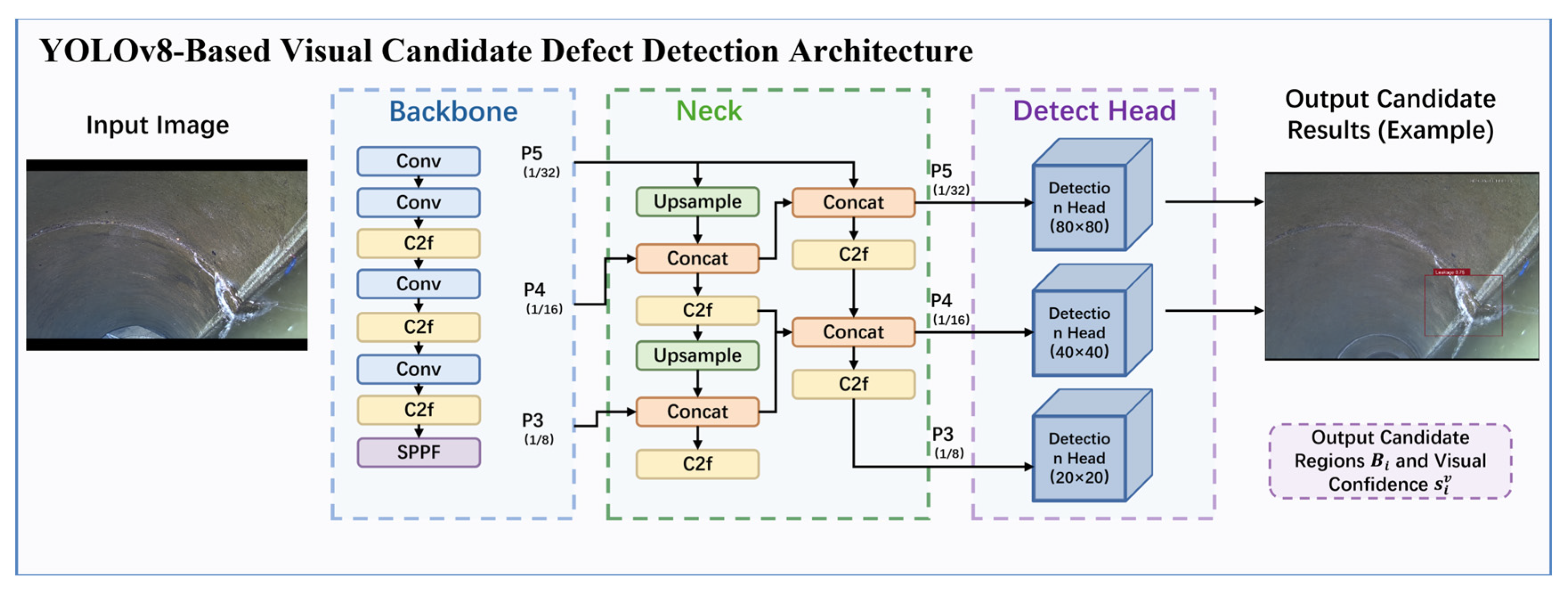
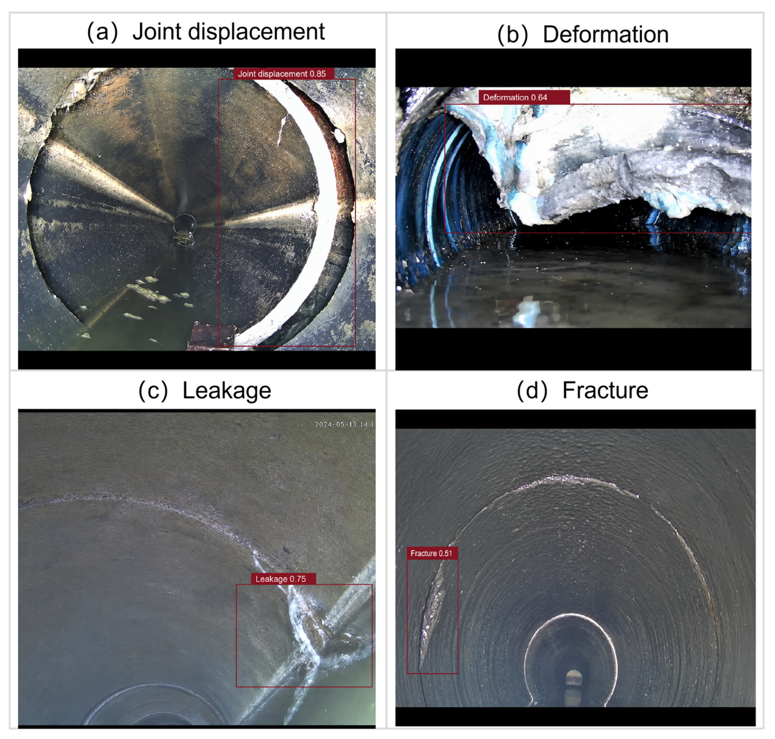
The vision module is used as one of the three independent candidate-generation branches. Considering the real-time processing and edge-deployment requirements of drainage pipeline inspection, YOLOv8n is adopted as the lightweight visual candidate-region generator, as illustrated in Figure 3. The YOLO architecture performs object localization and category prediction in a single-stage framework and is therefore suitable for rapid screening of surface defects such as cracks, corrosion, and joint misalignment [37,38,39,40]. In the model used in this study, a Convolutional Block Attention Module (CBAM) is inserted into the feature-extraction network to strengthen the response to fine cracks, weakly textured defects, and localized corrosion while suppressing complex pipe-wall background interference [41]. The absence of a visual candidate does not terminate the inspection pipeline; LiDAR- or ultrasonic-originated candidates are still processed according to Section 2.2.

Let the input image be denoted by $I_t$. The set of candidate defects output by the visual detection model is expressed as:

$${\mathrm{B}}_t=\{B_i{\}}_{i=1}^{N_t}$$

(3)

where the $i$-th candidate defect is represented as:

$$B_i=\left(x_i,y_i,w_i,h_i,c_i,s_i^v\right)$$

(4)

where $x_i$ and $y_i$ denote the center coordinates of the candidate bounding box, $w_i$ and $h_i$ denote its width and height, respectively, $c_i$ denotes the predicted defect class, $s_i^v\in \left[0,1\right]$ denotes the visual detection confidence score, and $N_t$ denotes the number of candidate defects in the current image frame.

With CBAM incorporated into the visual feature-extraction network, given an intermediate feature map $F\in {\mathbb{R}}^{C\times H\times W}$, the channel attention and spatial attention are expressed as follows:

$$F_c=M_c\left(F\right)\otimes F$$

(5)

$$F_s=M_s\left(F_c\right)\otimes F_c$$

(6)

where $M_c\left(\cdot \right)$ denotes the channel attention weights, $M_s\left(\cdot \right)$ denotes the spatial attention weights, and $\otimes$ represents element-wise multiplication. The attention mechanism enhances the feature responses of defect-related regions while suppressing interference from background textures and noise. However, the visual detection confidence cannot be directly regarded as the final defect confidence. To account for the influence of image quality on the detection results, the visual reliability coefficient is defined as:

$${\rho }_i^v={\gamma }_1{\tilde{L}}_i+{\gamma }_2{\tilde{C}}_i^{\mathrm{i}\mathrm{m}\mathrm{g}}+{\gamma }_3\left(1-{\tilde{R}}_i\right)+{\gamma }_4\left(1-{\tilde{O}}_i\right), {\displaystyle \sum _{k=1}^4}{\gamma }_k=1$$

(7a)

where ${\tilde{L}}_i, {\tilde{C}}_i^{img}, {\tilde{R}}_i, \mathrm{a}\mathrm{n}\mathrm{d}{\tilde{O}}_i$ are the normalized local illumination, image-contrast, reflection, and occlusion descriptors, respectively. The non-negative coefficients ${\gamma }_1-{\gamma }_4$ sum to one, so ${\rho }_i^v\in \left[0,1\right]$. The superscript ‘img’ prevents the image-contrast symbol from being confused with the fused defect confidence $C_i$ defined later in Equation (44). Reflection and occlusion enter through their complements because they reduce visual reliability.

$$L_i={\displaystyle \frac{1}{N_i^{\mathrm{p}\mathrm{i}\mathrm{x}}}}\sum _{p\in {\mathsf{\Omega }}_i}I\left(p\right)$$

(7b)

$$C_i^{\mathrm{i}\mathrm{m}\mathrm{g}}=\sqrt{{\displaystyle \frac{1}{N_i^{\mathrm{p}\mathrm{i}\mathrm{x}}}}\sum _{p\in {\mathsf{\Omega }}_i}{\left[I\left(p\right)-L_i\right]}^2}$$

(7c)

$$R_i={\displaystyle \frac{N_i^{\mathrm{r}\mathrm{e}\mathrm{f}}}{N_i^{\mathrm{p}\mathrm{i}\mathrm{x}}}}$$

(7d)

$$O_i={\displaystyle \frac{N_i^{\mathrm{o}\mathrm{c}\mathrm{c}}}{N_i^{\mathrm{p}\mathrm{i}\mathrm{x}}}}$$

(7e)

Here, ${\mathsf{\Omega }}_i$ denotes the candidate image region, $N_i^{pix}$ is the total number of pixels in ${\mathsf{\Omega }}_i$, $I\left(p\right)$ is the 8-bit grayscale intensity, and $N_i^{ref}$ and $N_i^{occ}$ are the numbers of reflective and occluded pixels, respectively. The four descriptors are subsequently normalized to $[0, 1]$ using the procedure in Equation (47).

The following implementation settings were used in the experiments reported in this study. Reflective and occluded pixels are identified by the following fixed image-quality rules:

$$\begin{array}{ll}\mathrm{reflective}: & V\left(p\right)\ge 230\hspace{0.25em}\wedge \hspace{0.25em}S\left(p\right)\le 64,\\ \mathrm{occluded}: & I\left(p\right)\le 25\hspace{0.25em}\wedge \hspace{0.25em}\parallel \nabla I\left(p\right)\parallel \le 5, N_{cc}\ge 50.\end{array}$$

The visual anomaly score is then defined as:

$${S_{\mathrm{i}}}^{\mathrm{v}}={s_{\mathrm{i}}}^{\mathrm{v}}, 0\le {S_{\mathrm{i}}}^{\mathrm{v}}\le 1$$

(8)

The visual anomaly score is therefore the detector confidence itself; visual reliability is not multiplied into $S_i^v$ at this stage and is applied only once when the basic probability assignment is constructed in Section 2.7. For a candidate initiated by LiDAR or ultrasonic sensing, the associated physical location is projected into the camera image using the calibrated camera–robot geometry, and $s_i^v$ is taken as the maximum pre-threshold defect confidence within the associated image region. Thus, failure to cross the visual candidate threshold does not make the visual evidence undefined. If the associated image region is unavailable or invalid, ${\rho }_i^v$ is set to zero.

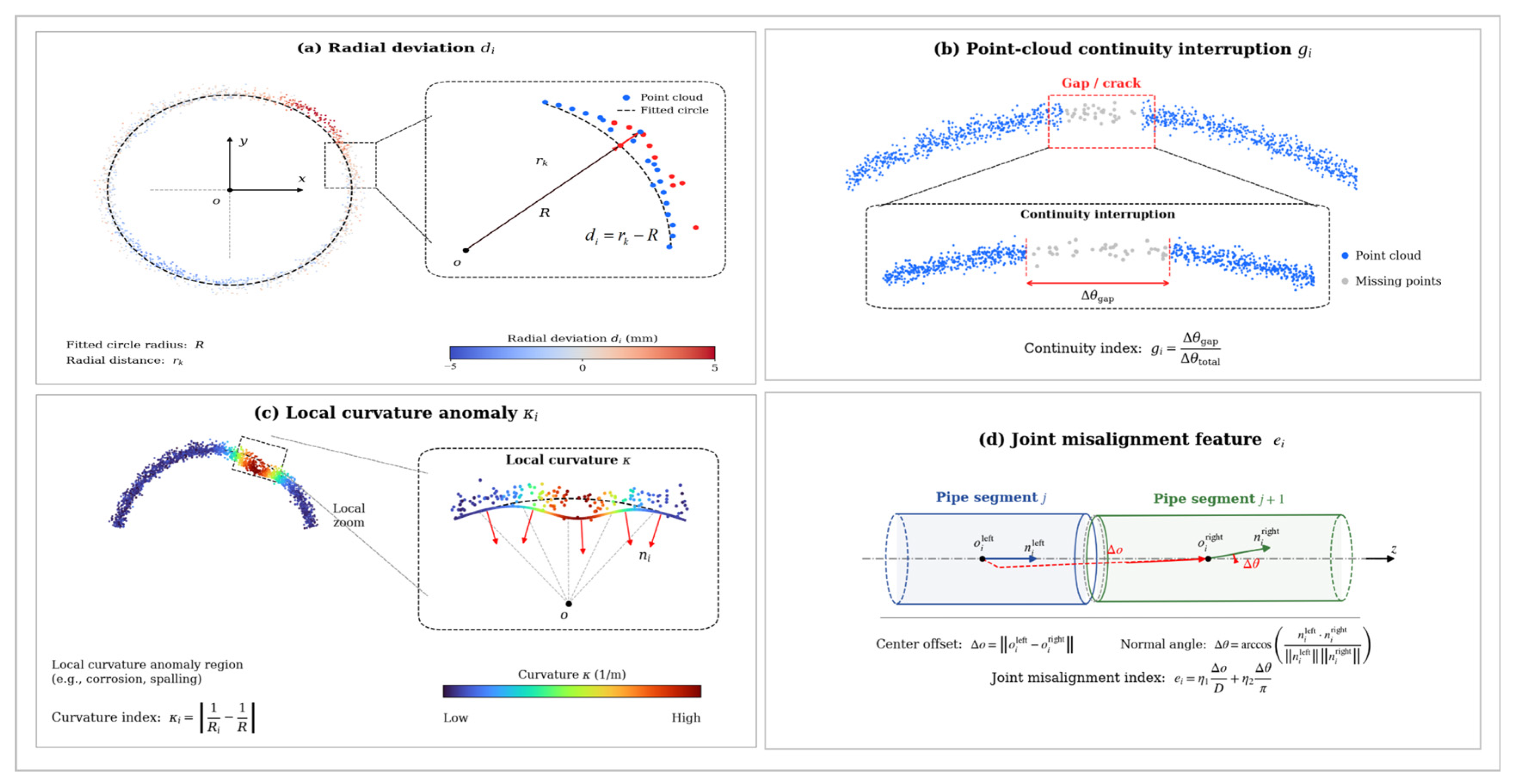
2.4. LiDAR Geometric Anomaly Screening and Verification

LiDAR point clouds serve two roles in the proposed framework: independent geometric anomaly screening and cross-modal verification. The LiDAR stream is continuously divided into spatially indexed local segments, and the geometric features described below are evaluated for every valid segment rather than only after a visual candidate has been generated. Segments exhibiting abnormal pipe-profile, curvature, continuity, or joint-displacement responses can therefore nominate LiDAR candidates independently. For candidates initiated by the visual or ultrasonic branch, the same LiDAR features are computed from the associated local point cloud. Unlike visual images, which primarily capture surface textures, LiDAR provides geometric information on the internal pipe profile, local deformation, and joint structures, making it suitable for identifying joint misalignment, local depressions, surface spalling, and pipe-wall deformation [24,25,30,31].

In the present framework, LiDAR is primarily employed as a complementary sensing modality for identifying macroscopic geometric anomalies, including pipe-wall deformation, local depressions, joint displacement, and other profile or continuity abnormalities. It is not intended to independently resolve fine surface defects, such as narrow cracks with negligible geometric variation. Accordingly, the LiDAR branch provides supporting geometric evidence rather than serving as a substitute for visual inspection of fine surface defects.

For the i-th candidate region, regardless of whether it was initiated by the visual, LiDAR, or ultrasonic branch, the corresponding local point cloud is obtained from the spatial association described in Section 2.2. For a LiDAR-originated candidate, the triggering point-cloud segment itself is used as the local segment:

$$P_i={\left\{p_k=\left(x_k,y_k,z_k\right)\right\}}_{k=1}^{M_i}$$

(9)

In the cross-sectional plane of the pipeline, the normal pipe-wall profile can be approximated by a circular-arc model:

$${\left(y-y_0\right)}^2+{\left(z-z_0\right)}^2=R^2$$

(10)

where $y_0$ and $z_0$ denote the coordinates of the center of the locally fitted cross-section, and $R$ denotes the pipe radius. By minimizing the residuals between the point-cloud points and the fitted circle, a reference model of the local pipe wall can be obtained as follows:

$$\underset{y_0,z_0,R}{\min }{\sum }_{p_k\in P_i}{\left(\sqrt{(y_k-y_0{)}^2+(z_k-z_0{)}^2}-R\right)}^2$$

(11)

On this basis, four types of geometric anomaly features are extracted.

First, the radial deviation feature is considered. Let the radial distance from point $p_k$ to the center of the locally fitted cross-section be defined as:

$$r_k=\sqrt{{\left(y_k-y_0\right)}^2+{\left(z_k-z_0\right)}^2}$$

(12)

The mean radial deviation of the candidate region is then defined as:

$$d_i={\displaystyle \frac{1}{M_i}}{\sum }_{p_k\in P_i}{\displaystyle \frac{\left|r_k-R\right|}{R}}$$

(13)

A larger radial deviation indicates a higher likelihood of local depressions, deformation, or profile anomalies within the candidate region.

Second, the local curvature anomaly feature is considered. Covariance analysis is performed on the neighboring point cloud of point $p_k$. Let the resulting eigenvalues be ordered as $0\le {\lambda }_1\le {\lambda }_2\le {\lambda }_3$; the local surface-variation curvature is then defined by Equation (14).

$${\kappa }_k={\displaystyle \frac{{\lambda }_1}{{\lambda }_1+{\lambda }_2+{\lambda }_3}}$$

(14)

The mean curvature anomaly of the candidate region is defined as:

$${\kappa }_i={\displaystyle \frac{1}{M_i}}{\sum }_{p_k\in P_i}{\kappa }_k$$

(15)

The curvature anomaly is primarily used to characterize corrosion, spalling, surface roughening, and localized surface damage.

Third, the point-cloud continuity anomaly feature is considered. Let the actual point-cloud density within the candidate region be compared with a reference density estimated from the material- and diameter-matched training reference or, during field inference, from a robust local baseline computed from neighboring windows after excluding the current candidate interval. This avoids assuming that a neighboring test region is known a priori to be normal. The continuity anomaly is defined as:

$$g_i^l=\mathrm{c}\mathrm{l}\mathrm{i}\mathrm{p}\left(1-{\displaystyle \frac{n_i}{n_i^{\mathrm{r}\mathrm{e}\mathrm{f}}+\epsilon }},\hspace{0.25em}0,\hspace{0.25em}1\right)$$

(16)

A larger $g_i^l$ indicates a higher likelihood of a macroscopic crack-related gap, local interruption, missing-return structure, or other coherent surface discontinuity. The clipping in Equation (16) prevents densities above the reference level from producing negative anomaly values and $\epsilon$ prevents division by zero. Because the 16-beam LiDAR does not resolve fine crack width directly, $g_i^l$ is interpreted as supporting geometric/continuity evidence rather than as a stand-alone measurement of sub-centimeter crack geometry.

Fourth, the joint misalignment feature is considered. For a pipe-joint region, the local cross-sections on both sides of the joint are fitted separately, and the center offset and the angle between their normal vectors are calculated as follows:

$$\begin{array}{ll}{d}_i^{\mathrm{j}\mathrm{o}\mathrm{i}\mathrm{n}\mathrm{t}}& =\mathrm{c}\mathrm{l}\mathrm{i}\mathrm{p}\left({\displaystyle \frac{\parallel o_i^{\mathrm{l}\mathrm{e}\mathrm{f}\mathrm{t}}-o_i^{\mathrm{r}\mathrm{i}\mathrm{g}\mathrm{h}\mathrm{t}}\parallel }{R}},0,1\right),\\ {\varphi }_i^{\mathrm{j}\mathrm{o}\mathrm{i}\mathrm{n}\mathrm{t}}& ={\displaystyle \frac{1}{\pi }}\mathrm{a}\mathrm{r}\mathrm{c}\mathrm{c}\mathrm{o}\mathrm{s}\left({\displaystyle \frac{n_i^{\mathrm{l}\mathrm{e}\mathrm{f}\mathrm{t}}\cdot n_i^{\mathrm{r}\mathrm{i}\mathrm{g}\mathrm{h}\mathrm{t}}}{\parallel n_i^{\mathrm{l}\mathrm{e}\mathrm{f}\mathrm{t}}\parallel \hspace{0.17em}\parallel n_i^{\mathrm{r}\mathrm{i}\mathrm{g}\mathrm{h}\mathrm{t}}\parallel }}\right),\\ \hspace{1em}{e}_i^l& ={\zeta }_1{d}_i^{\mathrm{j}\mathrm{o}\mathrm{i}\mathrm{n}\mathrm{t}}+{\zeta }_2{\varphi }_i^{\mathrm{j}\mathrm{o}\mathrm{i}\mathrm{n}\mathrm{t}}, {\zeta }_1+{\zeta }_2=1.\end{array}$$

(17)

where $o_i^{left}$ and $o_i^{right}$ denote the fitted cross-section centers on the two sides of a joint, and $n_i^{left} n_i^{right}$ denote the corresponding pipe-wall normal vectors. Equation (17) first converts center displacement and angular misalignment to dimensionless quantities before weighting them, avoiding the previous addition of a length directly to an angle. The fixed subweights used in the experiments are ${\zeta }_1={\zeta }_2=0.50$.

By integrating the geometric features described above, the LiDAR-based geometric anomaly score is defined as:

$$S_i^l={\alpha }_1{\tilde{d}}_i+{\alpha }_2{\tilde{\kappa }}_i+{\alpha }_3{\tilde{g}}_i^l+{\alpha }_4{\tilde{e}}_i^l, {\displaystyle \sum _{k=1}^4}{\alpha }_k=1$$

(18)

where ${\tilde{d}}_i, {\tilde{\kappa }}_i, {\tilde{g}}_i^l, \mathrm{a}\mathrm{n}\mathrm{d}{\tilde{e}}_i^l$ are the normalized radial-deviation, curvature, point-cloud-continuity, and joint-misalignment anomaly features. The superscript l distinguishes LiDAR-specific features from similarly named ultrasonic features. The non-negative coefficients ${\alpha }_1-{\alpha }_4$ sum to one; hence, the score is bounded within [0, 1].

The LiDAR reliability coefficient is defined as:

$${\rho }_i^l={\mu }_1{\tilde{N}}_i+{\mu }_2{Q}_i+{\mu }_3\left(1-H_i^{\mathrm{i}\mathrm{n}\mathrm{v}}\right), {\displaystyle \sum _{k=1}^3}{\mu }_k=1$$

(19a)

where ${\tilde{N}}_i$ is the normalized valid point density, $Q_i$ is the coverage completeness, and $H_i^{inv}$ is the acquisition-invalid ratio. Only invalid returns attributable to sensing/coverage failure (for example, out-of-FOV sampling, known occlusion, or packet/return loss) enter $H_i^{inv}$; coherent structural gaps used by $g_i^l$ are not counted again as reliability failures. The non-negative coefficients ${\mu }_1-{\mu }_3$ sum to one, so ${\rho }_i^l\in \left[0,1\right]$.

For reproducibility, the underlying LiDAR quality descriptors in Equation (19a) are computed as follows:

$$N_i=\mathrm{N}\mathrm{o}\mathrm{r}\mathrm{m}\left({\displaystyle \frac{n_i}{A_i^{\mathrm{s}\mathrm{u}\mathrm{r}\mathrm{f}}}}\right)$$

(19b)

$$Q_i={\displaystyle \frac{M_i^{\mathrm{v}\mathrm{a}\mathrm{l}\mathrm{i}\mathrm{d}}}{M_i}}$$

(19c)

$$H_i^{\mathrm{i}\mathrm{n}\mathrm{v}}={\displaystyle \frac{M_i^{\mathrm{i}\mathrm{n}\mathrm{v}\mathrm{a}\mathrm{l}\mathrm{i}\mathrm{d}}}{M_i}}$$

(19d)

Here, $n_i$ is the number of valid LiDAR points in the local candidate region, $A_i^{surf}$ is the fitted surface area, $M_i$ is the number of surface-grid cells, $M_i^{valid}$ is the number of cells containing valid returns, and $M_i^{invalid}$ is the number of cells invalid because of known acquisition/coverage failure. The raw point-density term is normalized according to Equation (47), whereas $Q_i$ and $H_i^{inv}$ are already bounded in $[0, 1]$. This definition separates a defect-related surface discontinuity from missing data caused by the sensor or viewing geometry.

For the experimental configuration, the locally fitted pipe-wall surface is divided into 25 mm × 25 mm grid cells rather than 10 mm × 10 mm cells. The coarser grid is intentionally chosen to avoid interpreting sub-sensor-scale fluctuations as structural voids given the RS-LiDAR-16 typical ranging accuracy reported in Section 3.1. A cell is valid when it contains at least one return. An empty cell is counted as an anomalous internal void only when at least five of its eight neighboring cells are valid; cells outside the LiDAR field of view or excluded by known physical occlusion are not counted in $M_i$. The 25 mm grid size is the setting used in the experiments and is supported by the measured point-density distribution and the sensor ranging characteristics (see Figure 4).

2.5. Ultrasonic Acoustic Anomaly Screening and Verification

Ultrasonic signals likewise serve both as an independent anomaly screening branch and as cross-modal confirmation evidence. Along the physical contact path of the spring-loaded probe, valid pulse-echo records are continuously evaluated for wall-thickness variation, abnormal echo amplitude, and spectral changes. An abnormal ultrasonic response can therefore initiate an acoustic candidate without requiring a visual bounding box at the same location. For candidates initiated by vision or LiDAR, the associated ultrasonic record is used as additional structural evidence. This mechanism is particularly relevant to wall-thickness reduction and internal or weakly visible damage [27,28]. Because the current platform uses a contact probe rather than a full-circumference ultrasonic array, independent ultrasonic candidate generation is explicitly limited to locations where stable coupling and probe coverage are available.

The applicability of contact-ultrasonic sensing is material dependent in the present study. For reinforced-concrete sections, ultrasonic responses are used primarily as auxiliary acoustic evidence when stable and repeatable echoes are available. For HDPE sections, where reliable probe coupling and identifiable back-wall echoes can be established, calibrated pulse-echo time-of-flight measurements can additionally support quantitative wall-thickness assessment.

Accordingly, all ultrasonic inspection results reported in this study are interpreted only for pipe-wall locations where the probe maintains effective physical contact and stable acoustic coupling and where the required acoustic features remain computable. Locations outside the calibrated probe-contact path, or locations at which stable coupling cannot be established, are treated as ultrasonic-unavailable rather than as negative ultrasonic observations.

Let the ultrasonic time-domain signal corresponding to the i-th candidate region be denoted by $u_i\left(t\right)$. Its frequency-domain representation is expressed as:

$$U_i\left(f\right)=\mathcal{F}\left\{u_i\left(t\right)\right\}$$

(20)

where $\mathcal{F}\left\{\cdot \right\}$ denotes the Fourier transform. Three types of acoustic anomaly features are extracted in this study.

First, the wall-thickness variation feature is considered. Let c denote the calibrated propagation velocity in the pipe-wall material and let $\Delta t_i$ denote the round-trip time difference between the front/interface echo and the back-wall echo. The local wall-thickness estimate is then given by Equation (21).

$$h_i={\displaystyle \frac{c\hspace{0.17em}\Delta t_i}{2}}$$

(21)

Let $h_{\mathrm{r}\mathrm{e}\mathrm{f}}$ denote the nominal/design wall thickness when available; otherwise, $h_{\mathrm{r}\mathrm{e}\mathrm{f}}$ is obtained from a material- and section-specific reference established during calibration or from a robust local baseline computed outside the current candidate interval. The reference is therefore determined without using the test label of an ‘adjacent normal region.’ The wall-thickness reduction ratio is then defined as:

$$r_i^u=\mathrm{c}\mathrm{l}\mathrm{i}\mathrm{p}\left({\displaystyle \frac{h_{\mathrm{r}\mathrm{e}\mathrm{f}}-h_i}{h_{\mathrm{r}\mathrm{e}\mathrm{f}}+\epsilon }},\hspace{0.25em}0,\hspace{0.25em}1\right)$$

(22)

A larger $r_i^u$ indicates a higher likelihood of wall-thickness loss. Equation (22) uses $h_{\mathrm{r}\mathrm{e}\mathrm{f}}$ consistently with the surrounding definition and clips negative or physically implausible reduction values to the admissible interval $[0, 1]$.

Second, the back-wall echo-amplitude anomaly feature is considered. Let $A_{\mathrm{r}\mathrm{e}\mathrm{f}}^{\mathrm{b}\mathrm{w}}$ denote the material- and section-specific reference back-wall amplitude obtained during calibration or from a robust local baseline outside the current candidate interval, and let $A_i^{\mathrm{b}\mathrm{w}}$ denote the candidate back-wall amplitude. The amplitude anomaly is defined by Equation (23). The superscript ‘bw’ distinguishes defect-sensitive back-wall attenuation from the front/interface echo used only for coupling-quality assessment.

$$a_i^u=\left|{\displaystyle \frac{A_{\mathrm{r}\mathrm{e}\mathrm{f}}^{\mathrm{b}\mathrm{w}}-A_i^{\mathrm{b}\mathrm{w}}}{A_{\mathrm{r}\mathrm{e}\mathrm{f}}^{\mathrm{b}\mathrm{w}}+\epsilon }}\right|$$

(23)

Variations in echo amplitude can reflect material attenuation, interface anomalies, or changes in the internal structure.

Third, the spectral-energy anomaly feature is considered. The normalized energy within the frequency band $\left[f_1,f_2\right]$ is defined as:

$$E_i\left(f_1,f_2\right)={\displaystyle \frac{{\int }_{f_1}^{f_2}{\left|U_i\left(f\right)\right|}^2\hspace{0.17em}df}{{\int }_0^{f_{\mathrm{m}\mathrm{a}\mathrm{x}}}{\left|U_i\left(f\right)\right|}^2\hspace{0.17em}df+\epsilon }}$$

(24)

If the spectrum is divided into $M_f$ frequency bands, the spectral anomaly of the candidate region can be expressed as:

$$e_i^u={\displaystyle \sum _{m=1}^{M_f}}{\omega }_m\left|E_i\left(f_m^1,f_m^2\right)-E_{\mathrm{r}\mathrm{e}\mathrm{f}}\left(f_m^1,f_m^2\right)\right|$$

(25)

where $E_{ref}$ denotes the reference spectral-energy distribution for each frequency band, obtained from material- and section-specific calibration/reference data or from a robust local baseline outside the current candidate interval. The band weights are non-negative and normalized to sum to one.

By integrating the acoustic features described above, the ultrasonic acoustic anomaly score is defined as:

$$S_i^u={\beta }_1{\tilde{r}}_i^u+{\beta }_2{\tilde{a}}_i^u+{\beta }_3{\tilde{e}}_i^u, {\displaystyle \sum _{k=1}^3}{\beta }_k=1$$

(26)

where ${\tilde{r}}_i^u, {\tilde{a}}_i^u, \mathrm{a}\mathrm{n}\mathrm{d}{\tilde{e}}_i^u$ are the normalized wall-thickness-reduction, back-wall-amplitude, and spectral-energy anomaly features. The modality superscript u avoids symbol collisions with LiDAR variables. The non-negative coefficients ${\beta }_1-{\beta }_3$ sum to one, so $S_i^u\in \left[0,1\right]$.

Meanwhile, to prevent low-quality ultrasonic signals from misleading the fusion results, the ultrasonic reliability coefficient is defined as:

$${\rho }_i^u={\delta }_1{\tilde{q}}_i^{\mathrm{S}\mathrm{N}\mathrm{R}}+{\delta }_2{\tilde{q}}_i^{\mathrm{c}\mathrm{p}\mathrm{l}}+{\delta }_3\left(1-{\tilde{\xi }}_i^{\mathrm{c}\mathrm{p}\mathrm{l}}\right), {\displaystyle \sum _{k=1}^3}{\delta }_k=1$$

(27a)

where ${\tilde{q}}_i^{SNR}, {\tilde{q}}_i^{cpl}, \mathrm{a}\mathrm{n}\mathrm{d} {\tilde{\xi }}_i^{cpl}$ are the normalized signal-to-noise, front/interface coupling-quality, and coupling-instability descriptors, respectively. The non-negative coefficients ${\delta }_1-{\delta }_3$ sum to one; hence ${\rho }_i^u\in \left[0,1\right]$. Defect-sensitive back-wall attenuation is used only in the anomaly score and is not reused as a reliability penalty. When the probe does not cover the candidate location according to Equation (2b), or when no valid acoustic features can be computed, ${\rho }_i^u$ is set to zero.

For reproducibility, the underlying ultrasonic quality descriptors in Equation (27a) are computed as follows:

$$q_i^{\mathrm{S}\mathrm{N}\mathrm{R}}=20{\mathrm{l}\mathrm{o}\mathrm{g}}_{10}\left({\displaystyle \frac{\mathrm{R}\mathrm{M}\mathrm{S}\left[u_i\left(t\right);W_s\right]}{\mathrm{R}\mathrm{M}\mathrm{S}\left[u_i\left(t\right);W_n\right]+\epsilon }}\right)$$

(27b)

$$q_i^{\mathrm{c}\mathrm{p}\mathrm{l}}=\mathrm{c}\mathrm{l}\mathrm{i}\mathrm{p}\left({\displaystyle \frac{A_i^{\mathrm{f}\mathrm{r}\mathrm{o}\mathrm{n}\mathrm{t}}}{A_{\mathrm{r}\mathrm{e}\mathrm{f}}^{\mathrm{f}\mathrm{r}\mathrm{o}\mathrm{n}\mathrm{t}}+\epsilon }},\hspace{0.25em}0,\hspace{0.25em}1\right)$$

(27c)

$${\xi }_i^{\mathrm{c}\mathrm{p}\mathrm{l}}={\displaystyle \frac{\sqrt{\frac{1}{K}{\displaystyle {\sum }_{k=1}^K}{\left(A_{i,k}^{\mathrm{f}\mathrm{r}\mathrm{o}\mathrm{n}\mathrm{t}}-{\overline{A}}_i^{\mathrm{f}\mathrm{r}\mathrm{o}\mathrm{n}\mathrm{t}}\right)}^2}}{{\overline{A}}_i^{\mathrm{f}\mathrm{r}\mathrm{o}\mathrm{n}\mathrm{t}}+\epsilon }}$$

(27d)

Here, $W_{s }\mathrm{a}\mathrm{n}\mathrm{d} W_n$ denote the signal and noise windows; RMS[·] denotes root-mean-square amplitude. $A_i^{front}$ is the front/interface echo amplitude used to assess probe coupling, $A_{ref}^{front}$ is its calibration/reference value, K is the number of consecutive A-scans, and ${\stackrel{-}{\mathrm{A}}}_i^{front}$ is their mean. Thus ${\xi }_i^{cpl}$ measures coupling stability rather than defect-sensitive back-wall attenuation.

The following signal-window settings are used in the experimental implementation:

$$W_s=\left[t_f-0.5\hspace{0.25em}\mathsf{\mu }\mathrm{s},\hspace{0.25em}{t}_f+0.5\hspace{0.25em}\mathsf{\mu }\mathrm{s}\right], W_n=\left[t_f-1.5\hspace{0.25em}\mathsf{\mu }\mathrm{s},\hspace{0.25em}{t}_f-0.5\hspace{0.25em}\mathsf{\mu }\mathrm{s}\right], K=5$$

(27e)

Accordingly, visually inconspicuous wall-thinning or internal-damage responses can be identified through the ultrasonic branch when the affected location intersects the probe-contact path and a stable echo is available. Ultrasonic evidence can therefore contribute independently of the visual candidate generator, while its effective coverage remains limited to physically inspected locations with reliable acoustic coupling.

2.6. Reproducible Comparison Baselines: Simple Weighted Fusion and Fixed-Weight D–S Fusion

All comparison baselines in Section 3.4 are defined on the same fixed test population. Let $a_i^j$ indicate hard modality availability for $j \in v,l,u: a_i^j = 1$ when the associated raw record exists, the candidate lies inside the modality’s physical coverage, and the modality-level score $S_i^j$can be computed; otherwise $a_i^j = 0$. This availability flag is deliberately separated from adaptive reliability. Poor-but-computable data therefore remain available $a_i^j = 1$ and are handled by ${\rho }_i^j$ only in the proposed method, whereas truly unavailable data are represented as ignorance in the D–S baselines.

$$a_i^j=\left\{\begin{array}{ll}1,& \mathrm{modality} j \mathrm{is} \mathrm{valid} \mathrm{at} \mathrm{candidate} i,\\ 0,& \mathrm{otherwise}.\end{array}\right.$$

(28)

For the simple weighted-fusion baseline, fixed modality priors ${\omega }_v$, ${\omega }_l$, and ${\omega }_u$ are renormalized only over modalities that are actually available at candidate i. Let $Z_i = {\Sigma }_k a_i^k {\omega }_k$. When $Z_i > 0$, Equation (29) yields normalized weights that sum to one. When $Z_i = 0$, no weighted score is computed and the baseline directly returns the not-confirmed output. This explicit edge-case rule avoids treating an all-unavailable candidate as if it had a meaningful zero-valued multimodal score.

$$Z_i=\sum _k{a}_i^k{\omega }_k, {\bar{\omega }}_i^j={\displaystyle \frac{a_i^j{\omega }_j}{Z_i}}\hspace{0.25em}\hspace{0.25em}\left(Z_i>0\right), \sum _j{\bar{\omega }}_i^j=1$$

(29)

The simple weighted score is then computed from the same modality anomaly scores used by the proposed method, without any adaptive reliability discount:

$$S_{\mathrm{i}}W={\Sigma }_{\mathrm{j}}\in \left\{v,l,u\right\}{{\stackrel{-}{\omega }}_{\mathrm{i}}}^{\mathrm{j}}{S_{\mathrm{i}}}^{\mathrm{j}}$$

(30)

The simple weighted baseline produces the same two operational outputs as the proposed method, using a single validation-selected threshold ${\tau }_W$:

$$Y_i^W=\left\{\begin{array}{ll}\mathrm{Confirmed} \mathrm{defect},& S_i^W\ge {\tau }_W,\\ \mathrm{Not} \mathrm{confirmed},& \mathrm{otherwise}.\end{array}\right.$$

(31)

For the fixed-weight D–S baseline, each available modality uses a constant discount factor ${\stackrel{-}{\rho }}_j$ that is independent of the current image, point-cloud, or ultrasonic quality. Its defect mass is:

$$m_{\mathrm{ij}}F\left(\left\{D\right\}\right)={a_{\mathrm{i}}}^{\mathrm{j}}{\stackrel{-}{\rho }}_{\mathrm{j}}{S_{\mathrm{i}}}^{\mathrm{j}}$$

(32)

The corresponding non-defect mass is:

$$m_{\mathrm{ij}}F\left(\left\{N\right\}\right)={a_{\mathrm{i}}}^{\mathrm{j}}{\stackrel{-}{\rho }}_{\mathrm{j}}\left(1-{S_{\mathrm{i}}}^{\mathrm{j}}\right)$$

(33)

The remaining mass is assigned to uncertainty:

$$m_{\mathrm{ij}}F\left(\left\{D,N\right\}\right)=1-{a_{\mathrm{i}}}^{\mathrm{j}}{\stackrel{-}{\rho }}_{\mathrm{j}}$$

(34a)

The fixed-weight D–S BPAs are combined using the same Dempster rule as Equation (41). The baseline confirms a defect when its fused defect mass $C_i^F$ reaches the validation-selected threshold ${\tau }_F$; otherwise the output is not confirmed. For completeness, the single-sensor baseline decision is written explicitly as:

$$Y_i^j=\left\{\begin{array}{ll}\mathrm{Confirmed} \mathrm{defect},& a_i^j=1\hspace{0.25em}\wedge \hspace{0.25em}{S}_i^j\ge {\tau }_j,\\ \mathrm{Not} \mathrm{confirmed},& \mathrm{otherwise},\end{array}\right. j\in \left\{v,l,u\right\}$$

(34b)

The two dual-sensor baselines use the following candidate unions and apply the availability-renormalized score in Equations (29) and (30) restricted to the named modalities:

$$B_V^L=B_v\cup B_l, B_V^U=B_v\cup B_u$$

(34c)

The three-modality simple weighted baseline uses Equations (28)–(31), whereas the fixed-weight D–S baseline uses Equations (32)–(34d). The operating values used in the experiments are:

$$\begin{array}{llllll} \mathsf{\omega }& =\left(\mathrm{0.40,0.35,0.25}\right),& \hspace{1em}& \hspace{1em}& \hspace{1em}& {\bar{\rho }}_v={\bar{\rho }}_l={\bar{\rho }}_u=0.80,\\ {\tau }_V& =0.50,& {\tau }_L& =0.52,& {\tau }_U& =0.50,\\ {\tau }_{VL}& =0.52,& {\tau }_{VU}& =0.51,& {\tau }_W& =0.52, {\tau }_F=0.55.\end{array}$$

(34d)

These thresholds are validation-selected operating points. Every method is still evaluated on all 105 test groups; differences in candidate union never change the evaluation denominator.

2.7. Reliability-Constrained D–S Evidence Fusion

To integrate the visual, LiDAR, and ultrasonic evidence into a unified decision framework, Dempster–Shafer (D–S) evidence theory is employed for multi-source information fusion [32,33]. D–S evidence theory is capable of combining multi-source information under uncertain conditions and is therefore suitable for defect confirmation in drainage pipelines affected by low illumination, standing water, reflections, and occlusions [34,35,36,42,43].

The frame of discernment is defined as:

$$\mathsf{\Theta } = \{\mathrm{D}, \mathrm{N}\}$$

(35)

where denotes $D$ “defect present” and $N$ denotes “no defect.” The corresponding power set is given by:

$$2^{\Theta }=\left\{\varnothing ,\left\{D\right\},\left\{N\right\},\{D,N\}\right\}$$

(36)

where represents $\left\{D,N\right\}$ the uncertain state.

For the i-th candidate region and the j-th sensor modality, the basic probability assignment function is constructed as follows:

$$m_i^j\left(\left\{D\right\}\right)={\rho }_i^j{S}_i^j$$

(37)

$$m_i^j\left(\left\{N\right\}\right)={\rho }_i^j\left(1-S_i^j\right)$$

(38)

$$m_i^j\left(\left\{D,N\right\}\right)=1-{\rho }_i^j$$

(39)

$$m_i^j\left(\varnothing \right)=0$$

(40)

where $j \in \left\{v,l,u\right\}$, $S_i^j \in [0, 1]$ is the modality-level anomaly score defined independently of reliability, and ${\rho }_i^j \in [0, 1]$ is the corresponding reliability coefficient. Reliability is applied exactly once in Equations (37)–(39): a reliable modality assigns more mass to defect/non-defect according to $S_i^j$, whereas an unreliable or unavailable modality shifts mass to the uncertainty set {D, N}.

For each union candidate, every modality that physically covers the associated location is evaluated even if it did not independently trigger that candidate. A valid non-triggering modality contributes to its pre-threshold anomaly score and reliability; it is neither forced to zero nor omitted merely because it failed to generate a candidate. If a modality is outside its physical coverage or its data are invalid, its reliability is set to zero and its entire BPA is assigned to uncertainty. In particular, Equation (2b) governs whether contact-ultrasonic evidence is available at a candidate location.

For two evidence sources $m_1$ and $m_2$, Dempster’s rule and its pairwise conflict coefficient are defined together in Equation (41):

$$\begin{array}{cc}{K}_{12}& =\sum _{B\cap C=⌀}{m}_1\left(B\right)m_2\left(C\right),\\ \left(m_1\oplus m_2\right)\left(A\right)& ={\displaystyle \frac{\sum _{B\cap C=A}{m}_1\left(B\right)m_2\left(C\right)}{1-K_{12}}}, A\ne ⌀.\end{array}$$

(41)

For the three-source decision used in this study, the conflict quantity entering the decision rule is defined as the total mass assigned by the three sources to mutually incompatible intersections:

$$K_i=\sum _{\begin{array}{c}{A}_v,A_l,A_u\in 2^{\Theta }\\ A_v\cap A_l\cap A_u=⌀\end{array}}{m}_i^v\left(A_v\right)m_i^l\left(A_l\right)m_i^u\left(A_u\right)$$

(42)

For $K_i<1$, the three-source fused BPA is computed directly using the same normalized intersection rule, with the global conflict $K_i$ from Equation (42):

The classical Dempster combination rule is most appropriate when the evidence sources can be treated as sufficiently distinct and approximately independent. In practical drainage-pipeline environments, however, the visual, LiDAR, and ultrasonic evidence may not be strictly statistically independent because shared environmental disturbances can affect more than one sensing channel. For example, standing water or high humidity may simultaneously alter visual appearance and ultrasonic coupling conditions, while surface contamination may influence both image texture and local geometric observations. Accordingly, the three sensing modalities are regarded in this study as physically complementary rather than strictly independent. The current formulation does not explicitly estimate cross-modal statistical dependence. It should also be noted that the conflict coefficient K primarily characterizes disagreement among evidence sources and does not, by itself, quantify statistical dependence or common-mode bias. Therefore, correlated evidence affected by the same environmental disturbance may still be over-reinforced during D–S combination.

$$m_i^f\left(A\right)=\left\{\begin{array}{ll}{\displaystyle \frac{\sum _{\begin{array}{c}{A}_v,A_l,A_u\in 2^{\Theta }\\ A_v\cap A_l\cap A_u=A\end{array}}{m}_i^v\left(A_v\right)m_i^l\left(A_l\right)m_i^u\left(A_u\right)}{1-K_i}},& A\ne ⌀,\\ 0,& A=⌀.\end{array}\right.$$

(43)

If $K_i = 1$, Dempster normalization is undefined; in that case no normalized fused BPA is computed and the candidate is directly assigned to the not-confirmed decision. This explicit rule prevents division by zero under complete evidence conflict.

The final defect confidence is defined as:

$$C_i=m_i^f\left(D\right)$$

(44)

The uncertainty is defined as:

$$U_i=m_i^f\left(\left\{D,N\right\}\right)$$

(45)

To convert the fused evidence into a binary confirmation result while preventing high-conflict or high-uncertainty evidence from being accepted as a defect, a conflict- and uncertainty-constrained decision rule is introduced:

$$Y_i=\left\{\begin{array}{ll}\mathrm{Confirmed} \mathrm{defect},& C_i\ge {\tau }_c,\hspace{0.25em}{U}_i<{\tau }_u,\hspace{0.25em}{K}_i<{\tau }_k,\\ \mathrm{Not} \mathrm{confirmed},& \mathrm{otherwise}.\end{array}\right.$$

(46a)

where ${\tau }_c$ denotes the defect-confirmation threshold, ${\tau }_u$ the uncertainty threshold, and ${\tau }_k$ the evidence-conflict threshold. The negative system output is termed ‘not confirmed’ rather than ‘non-defect’ because high uncertainty or conflict does not constitute positive evidence that the region is defect-free. For group-level evaluation, let $C_g$ denote the set of all union candidates assigned to evaluation group g. A group is positive if any candidate within that group is confirmed:

$$Y_g=\left\{\begin{array}{ll}\mathrm{Confirmed} \mathrm{defect},& \exists i\in {\mathcal{C}}_g:\hspace{0.25em}{Y}_i=\mathrm{Confirmed} \mathrm{defect},\\ \mathrm{Not} \mathrm{confirmed},& {\mathcal{C}}_g=⌀\hspace{0.25em}\mathrm{or} \mathrm{all} i\in {\mathcal{C}}_g \mathrm{are} \mathrm{not} \mathrm{confirmed}.\end{array}\right.$$

(46b)

Therefore, a defect group receiving ‘not confirmed’ is a false negative, while a non-defect group receiving ‘not confirmed’ is a true negative. If a group contains no candidate, $C_g$ is empty and the group-level output is not confirmed.

2.8. Parameter Domains and Validation-Based Selection Rules

To make the parameterization explicit, the feature normalization procedure, admissible parameter domains, weighting constraints, and validation-based selection rules are specified below. First, all visual, geometric, and acoustic features are normalized to the interval $\left[0,1\right]$ as follows:

$${\tilde{x}}_{\mathrm{i}}=clip\left[{\displaystyle \frac{x_{\mathrm{i}}-{x_{\min }}^{\mathrm{tr}}}{{x_{\max }}^{\mathrm{tr}}-{x_{\min }}^{\mathrm{tr}}+\epsilon }},0,1\right]$$

(47)

where $x_i$ denotes the original feature value, $x_{min}^{tr}$ and $x_{max}^{tr}$ are estimated from the training subset only and then frozen, $\epsilon$ is a small positive constant, and $clip\left(·,0,1\right)$ truncates values outside the training range to the admissible interval. The clipping operation is necessary because a validation or test observation can legitimately fall below the training minimum or above the training maximum; without clipping, Equation (47) would contradict the stated $[0, 1]$ domains of the downstream anomaly and reliability scores. No validation- or test-set extrema are used for rescaling.

Second, the feature and reliability weights in Equations (7), (18), (19a), (26) and (27) are treated as fixed engineering priors rather than parameters optimized on the small validation subset. The same applies to the fixed modality weights used by the comparison baselines in Section 2.6. All such weights are non-negative and normalized within each group to sum to one, ensuring scores and reliability coefficients remain in $[0, 1]$. For the proposed method, only six operating thresholds are selected from data: the three branch-screening thresholds ${\eta }_v$, ${\eta }_l$, and ${\eta }_u$ and the three final decision thresholds ${\tau }_c$, ${\tau }_u$, and ${\tau }_K$. This restriction prevents the 18-defect validation subset from being used to tune dozens of continuous coefficients. Baseline decision thresholds ${\tau }_W$ and ${\tau }_F$ are selected separately on validation for their own methods and do not affect the proposed method.

$$\begin{array}{ll}{\mathcal{G}}_{\eta }& =\{\mathrm{0.05,0.10},\dots ,0.80\},\\ F_2& ={\displaystyle \frac{5PR}{4P+R}},\\ {\eta }_j^{\ast }& =\mathrm{a}\mathrm{r}\mathrm{g}\underset{{\eta }_j\in {\mathcal{G}}_{\eta }}{\mathrm{m}\mathrm{a}\mathrm{x}}{F}_{2,\mathrm{v}\mathrm{a}\mathrm{l}}^{\left(j\right)}\left({\eta }_j\right), j\in \{v,l,u\}.\end{array}$$

(48)

The branch-specific candidate thresholds are selected on the 105 validation region groups using the recall-emphasized $F_2$ criterion and the pre-specified finite search grid shown explicitly in Equation (48). A validation group is branch-positive when that branch nominates at least one spatially associated candidate belonging to the group. For ultrasonic screening, $F_2$ is computed only among groups whose labeled region intersects the calibrated probe-coverage path; uncovered groups are marked unavailable rather than acoustic negatives. Ties are resolved by higher Recall and then by the lower threshold.

Finally, the proposed decision vector $\tau =\left({\tau }_c,{\tau }_u,{\tau }_k\right)$ is selected jointly using only the validation subset. Equation (49) now defines the finite grid mathematically rather than using the inconsistent continuous domain ${\left[0,1\right]}^3$. Candidate triples are ranked first by validation $F_1$, then by the Youden index, then by higher Recall; any remaining tie is resolved deterministically by lower ${\tau }_c$, then higher ${\tau }_u$, then higher ${\tau }_k$. No threshold is refined between grid points after inspection of the test set.

$$\begin{array}{ll}{\mathcal{G}}_c& =\{\mathrm{0.40,0.45},\dots ,0.80\},\\ {\mathcal{G}}_u& =\{\mathrm{0.20,0.25},\dots ,0.70\},\\ {\mathcal{G}}_k& =\{\mathrm{0.40,0.45},\dots ,0.90\},\\ {\mathcal{G}}_{\tau }& ={\mathcal{G}}_c\times {\mathcal{G}}_u\times {\mathcal{G}}_k,\\ {\mathsf{\tau }}^{\ast }& =\mathrm{a}\mathrm{r}\mathrm{g}\underset{\mathsf{\tau }\in {\mathcal{G}}_{\tau }}{\mathrm{m}\mathrm{a}\mathrm{x}}{F}_{1,\mathrm{v}\mathrm{a}\mathrm{l}}\left(\mathsf{\tau }\right).\end{array}$$

(49)

During test evaluation, no feature normalization range, fusion weight, candidate threshold, merge window, or decision threshold is modified using the test subset. In the experimental configuration, fixed engineering priors and validation-selected operating points are listed separately in

Table 1. Fixed engineering priors and validation-selected operating settings used in the experiments.

Parameter Group	Equation(s)	Experimental Value	Source/Interpretation
Association metric	Equation (2a)	${\lambda }_t = 0.35$; ${\lambda }_s = 0.65$; ${\Delta t}_{max} = 50 \mathrm{m}\mathrm{s}$; ${\Delta s}_{max} = 30 \mathrm{m}\mathrm{m}$	λ fixed prior; temporal tolerance from acquisition protocol; spatial window fixed/calibration
Candidate-screening thresholds	Equation (48)	${\eta }_v = 0.20$; ${\eta }_l = 0.30$; ${\eta }_u = 0.25$	validation-selected with branch-wise F2; ultrasonic only within valid coverage
Cross-branch candidate merge	Section 2.2	${\Delta s}^B = 40 \mathrm{m}\mathrm{m}$; ${\Delta \mathcal{l}}^B = 40 \mathrm{m}\mathrm{m}$	fixed engineering window in common pipe coordinates
Ultrasonic coverage footprint	Equation (2b)	${\Delta s}_u = 15 \mathrm{m}\mathrm{m}$; ${\Delta \mathcal{l}}_u = 10 \mathrm{m}\mathrm{m}$	fixed/calibrated probe footprint used in the experiments
Visual reliability	Equation (7a)	${\gamma }_1 = 0.30$; ${\gamma }_2 = 0.25$; ${\gamma }_3 = 0.25$; ${\gamma }_4 = 0.20$	fixed engineering prior; $\Sigma \gamma = 1$
LiDAR anomaly score	Equation (18)	$\alpha = (0.25, 0.20, 0.25, 0.30)$; $\zeta = (0.50, 0.50)$	fixed priors; $\Sigma \alpha = 1$; ${\zeta }_1 + {\zeta }_2 = 1$; dimensionless joint terms
LiDAR reliability	Equation (19a)	${\mu }_1 = 0.30$; ${\mu }_2 = 0.45$; ${\mu }_3 = 0.25$	fixed engineering prior; $\Sigma \mu = 1$
Ultrasonic anomaly score	Equation (26)	${\beta }_1 = 0.50$; ${\beta }_2 = 0.30$; ${\beta }_3 = 0.20$	fixed engineering prior; $\Sigma \beta = 1$
Ultrasonic reliability	Equation (27a)	${\delta }_1 = 0.40$; ${\delta }_2 = 0.35$; ${\delta }_3 = 0.25$	fixed prior; $\Sigma \delta = 1$; SNR + coupling + stability
Single-/dual-sensor baselines	Section 2.6	${\tau }_V = 0.50$; ${\tau }_L = 0.52$; ${\tau }_U = 0.50$; ${\tau }_{VL} = 0.52$; ${\tau }_{VU} = 0.51$	validation-selected thresholds; all 105 test groups retained
Simple weighted baseline	Equations (28)–(31)	${\omega }_v = 0.40$; ${\omega }_l = 0.35$; ${\omega }_u = 0.25$; ${\tau }_W$ = 0.52	weights fixed; ${\tau }_W$ validation-selected; availability-renormalized
Fixed-weight D–S baseline	Equations (32)–(34d)	${\stackrel{-}{\rho }}_v = {\stackrel{-}{\rho }}_l = {\stackrel{-}{\rho }}_u = 0.80$; ${\tau }_F$ = 0.55	constant discount factors; ${\tau }_F$ validation-selected
Proposed decision thresholds	Equation (46)	${\tau }_c$ = 0.55; ${\tau }_u$ = 0.45; ${\tau }_k$ = 0.70	validation-selected jointly by F1; Youden tie-break
Feature normalization	Equation (47)	xmin/xmax from training only	frozen before validation and test; prevents rescaling leakage
Threshold search grids	Equations (48) and (49)	$\eta$: 0.05–0.80 by 0.05; ${\tau }_c$: 0.40–0.80; ${\tau }_u$: 0.20–0.70; ${\tau }_k$: 0.40–0.90 (all by 0.05)	pre-specified validation-only grids; deterministic tie-breaking; no test-set refinement

so that the source of every parameter is explicit. Values labeled ‘fixed prior/calibration’ are not optimized on validation, whereas values labeled ‘validation-selected’ are chosen before test evaluation. All numerical settings reported here correspond to the calibration and validation values used in the experiments (see Figure 5).

The algorithm receives synchronized pipeline images, LiDAR point-cloud segments, ultrasonic records, and fixed operating parameters as inputs. The three sensing branches generate candidates independently using ${\eta }_v$, ${\eta }_l$, and ${\eta }_u$; candidates are transformed to the common$(s,\theta )$ coordinate and merged only within the fixed spatial windows ${\Delta s}^B$ and ${\Delta \mathcal{l}}^B$. For each union candidate, associated modality data are retrieved using Equation (2a), while contact-ultrasonic availability is additionally checked by Equation (2b). The modality anomaly scores are computed independently of sensor reliability, and reliability is applied exactly once when constructing the proposed BPAs in Equations (37)–(39). The proposed D–S method then combines these adaptive BPAs directly. Section 2.6 defines separate class-independent comparison baselines using the same candidates and modality scores, ensuring that performance differences arise from the fusion rule rather than from different test populations or candidate availability. The final proposed decision follows Equation (46), yielding confirmed defect or not confirmed.

3. Experiments and Results

This section presents the experimental validation of the proposed vision–LiDAR–ultrasonic fusion method for defect confirmation. Since the primary objective of this study is to improve the reliability of defect confirmation in complex drainage pipeline environments rather than to emphasize millimeter-level spatial localization, the experimental design focuses on five aspects: the experimental platform and data acquisition, dataset construction and defect annotation, evaluation metrics, visual candidate detection performance, and multi-sensor fusion performance for defect confirmation.

3.1. Experimental Platform and Data Acquisition

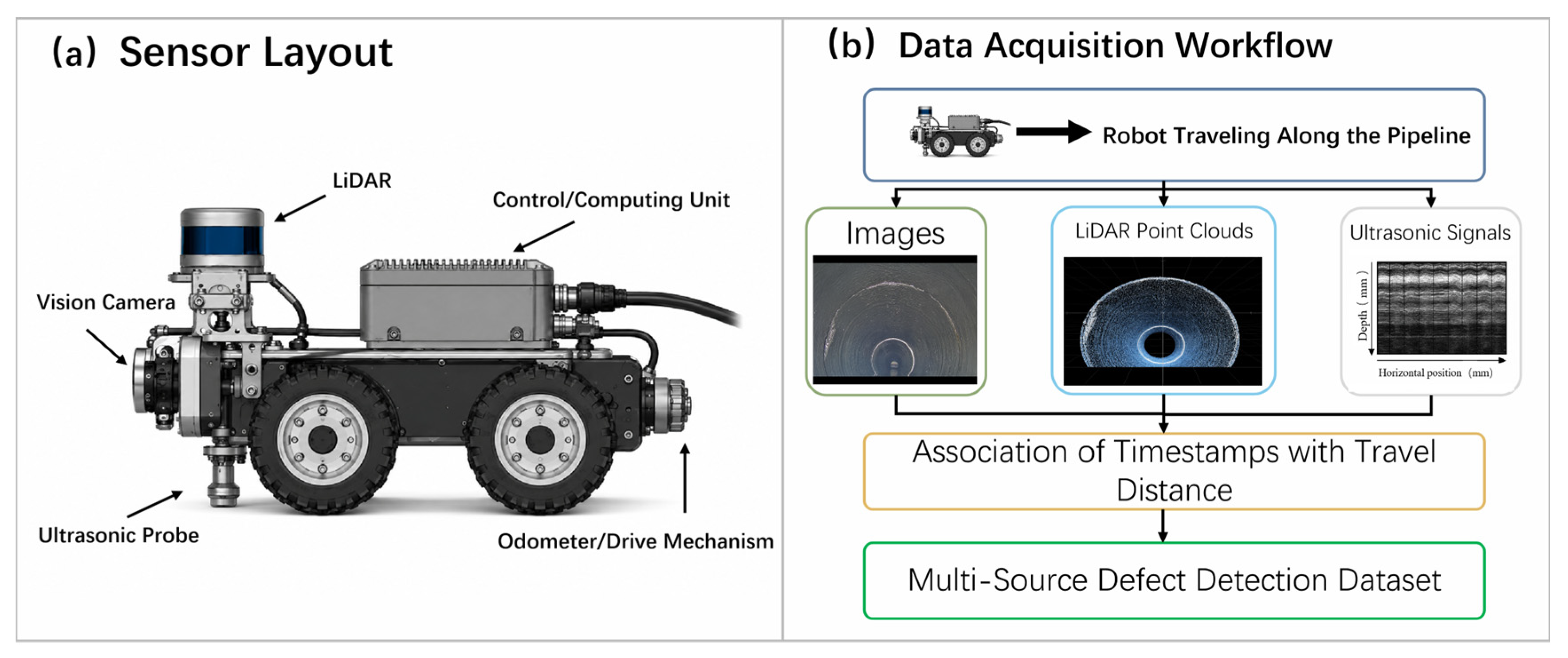
To validate the effectiveness of the proposed method in internal drainage-pipeline inspection scenarios, the experimental platform was configured as a four-wheel pipeline inspection robot carrying an IP67 color industrial camera (Basler ace 2 R a2A1920-51gcIP67, Basler AG, Ahrensburg, Germany), a 16-beam three-dimensional LiDAR (RoboSense RS-LiDAR-16, RoboSense Technology Co., Ltd., Shenzhen, China), an ultrasonic flaw detector (Evident EPOCH 650, Evident Scientific, Inc., Waltham, MA, USA) connected to an M106-RM 2.25 MHz (Evident Scientific, Inc., Waltham, MA, USA) contact transducer, an OMRON E6B2-CWZ6C 200 P/R (OMRON Corporation, Kyoto, Japan) incremental encoder, a continuous LED ring illumination unit, and an NVIDIA Jetson Xavier NX 8 GB (NVIDIA Corporation, Santa Clara, CA, USA) embedded computing platform. The camera provided visible surface information, the LiDAR provided local three-dimensional geometry and pipe-profile information, and the ultrasonic channel provided pulse-echo evidence for wall-thickness variation and internal acoustic anomalies. The specific hardware models, manufacturer-rated specifications, and acquisition settings are summarized in

Table 2. Hardware models, manufacturer-rated specifications, and acquisition settings of the multi-sensor inspection platform.

Module	Equipment/Parameters	Acquired Data	Main Function	Remarks
Visual camera	Basler ace 2 R a2A1920-51gcIP67; Sony IMX392 (Sony Semiconductor Solutions Corporation, Atsugi, Japan); 1920 × 1200; 51 fps max.; GigE; IP67	RGB images	Visual candidate detection	1920 × 1080 ROI; 30 fps; exposure/gain locked; LED ring illumination
LiDAR	RoboSense RS-LiDAR-16; 16 beams; 905 nm; 360° × 30° FoV; ±20 mm typical accuracy; 150 m max. range	3D point clouds	Geometry verification	10 Hz; rigid mounting retained during each inspection campaign
Ultrasonic system	Evident EPOCH 650 + M106-RM; 2.25 MHz; 13 mm element; 0.2–26.5 MHz receiver	A-scan echoes	Acoustic verification	Pulse-echo; PRF 1 kHz; material-specific velocity/zero calibration; water couplant; stable back-wall echo required
Odometer/encoder	OMRON E6B2-CWZ6C; 200 P/R; A/B/Z; 5–24 VDC; 100 mm odometer wheel	Travel distance	Data association	100 Hz; ≈1.57 mm/pulse; scale calibrated over a 5.0 m reference distance
Computing platform	NVIDIA Jetson Xavier NX 8 GB; 6-core Carmel CPU; 384-core Volta GPU + 48 Tensor Cores	Inference/records	Evidence fusion	15 W mode; common host clock for timestamping and data association
Inspection robot/motion	Four-wheel crawler; nominal axial speed 0.20 m/s	Motion state	Stable acquisition	Constant-speed inspection; speed used for synchronization-to-distance conversion
Illumination	Robot-mounted 12 V continuous LED ring; neutral white (~5000 K)	Local lighting	Image acquisition	Continuous during each run; no external ambient lighting

.

During data acquisition, the robot traveled along the pipe axis at a nominal speed of 0.20 m/s. The pipe interior was otherwise unlit, and the robot-mounted LED ring was used as the sole illumination source. Camera exposure and gain were initialized automatically at the beginning of each run and then locked to avoid frame-to-frame brightness drift; RGB images were recorded at 1920 × 1080 pixels and 30 fps. The RS-LiDAR-16 was operated at 10 Hz, and the ultrasonic instrument used pulse-echo acquisition with a 1 kHz pulse-repetition frequency. Encoder counts were sampled at 100 Hz. The camera, LiDAR, ultrasonic, and encoder channels were recorded continuously throughout each inspection run; visual detections were not used to start or stop the acquisition of the non-visual sensing streams. All data streams were assigned timestamps from the Jetson host clock and were associated using both timestamp proximity and encoder-derived travel distance. Associations with an absolute inter-sensor timestamp difference greater than 50 ms were rejected; at 0.20 m/s, this criterion limits synchronization-induced axial mismatch to 10 mm.

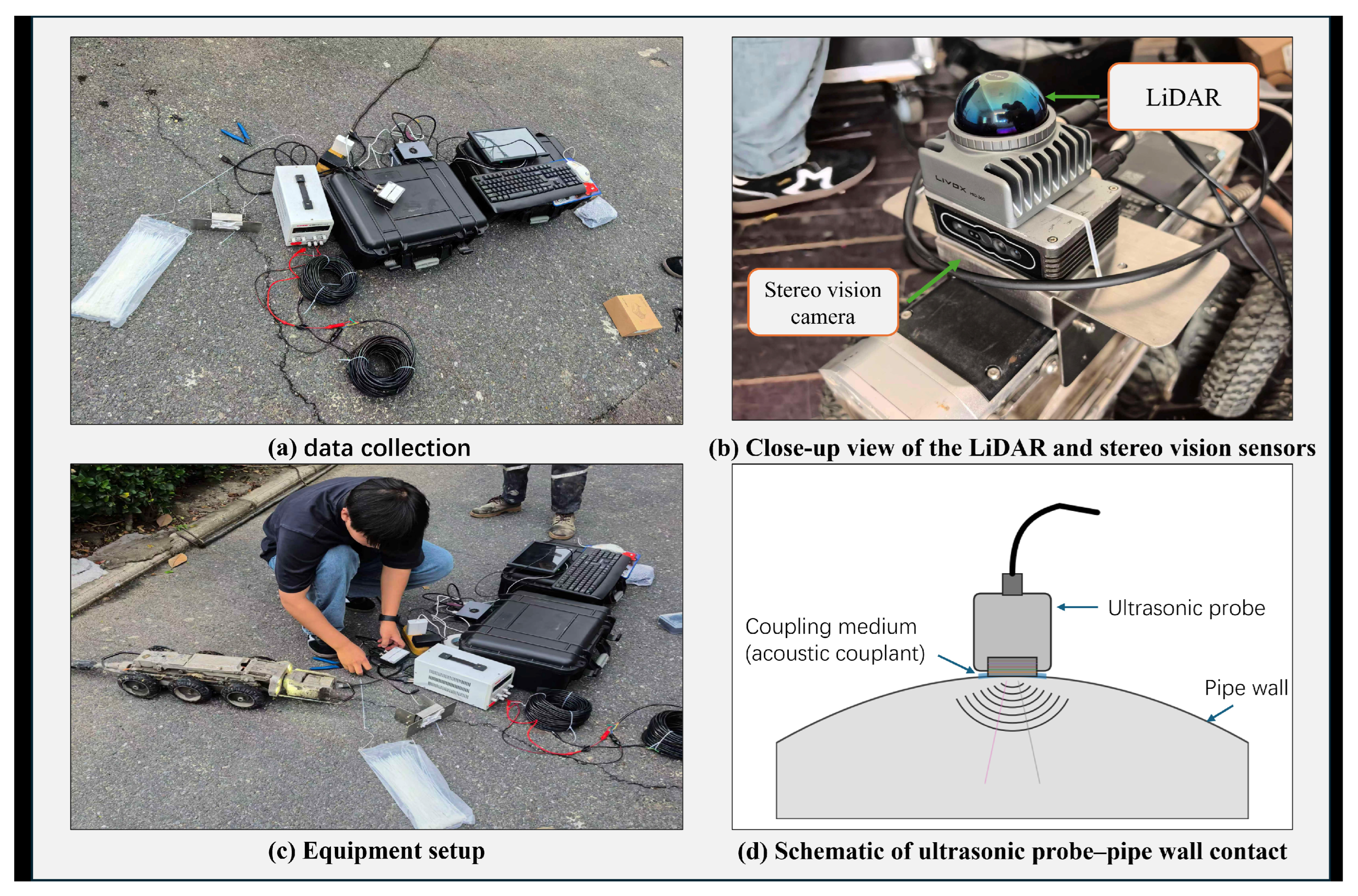
The sensors were rigidly mounted on the same robot frame. The camera was placed at the front center with its optical axis approximately aligned with the pipe axis, the LiDAR was mounted on the upper centerline, and the ultrasonic transducer was installed in a spring-loaded contact holder approximately normal to the local pipe wall. A robot-centered reference frame was used for all extrinsics. The local pipe centerline and cross-section fitted from LiDAR define the cylindrical coordinates $(s,\theta )$: s is axial distance along the fitted centerline and $\theta$ is the circumferential angle about that centerline. Visual candidate centers are mapped to the pipe surface through the calibrated camera-to-robot/LiDAR geometry, whereas the ultrasonic contact point has a calibrated robot-frame position and circumferential track ${\theta }^u\left(s\right)$. This explicit geometry is required so that the arc-length coverage test in Equation (2b) refers to the same physical pipe-wall location for all three modalities.

Calibration was performed before each inspection campaign. Camera intrinsic parameters were estimated with a planar checkerboard and lens distortion was removed before visual detection. The camera-to-LiDAR rigid transformation was obtained from a target observable in both modalities, and the resulting transform together with the measured sensor-to-robot mounting offsets was used to express camera and LiDAR observations in the common robot frame. The encoder scale factor was calibrated over a 5.0 m reference travel distance. For the ultrasonic channel, acoustic velocity and zero offset were calibrated using a reference coupon of the same pipe material and known thickness; in addition, the probe-contact point and circumferential track relative to the robot frame were calibrated on a reference pipe section, and the usable axial/circumferential footprint used in Equation (2b) was measured from the region over which stable repeatable echoes were obtained. A water-based couplant was applied at the probe–wall interface. Weak or unstable echoes are retained as low-quality observations when their features remain computable and are down-weighted by ${\rho }_i^u$; only records for which the required acoustic features cannot be computed at all are treated as unavailable and assigned ${\rho }_i^u = 0$. The reported footprint values correspond to the calibration results used in the experiments. Figure 6 summarizes the sensor layout and multi-source acquisition workflow, whereas Figure 7 provides representative field photographs of the experimental setup and sensor mounting together with a schematic of the ultrasonic probe–pipe wall contact condition. Because an independent metrology system was not available for absolute field registration-error measurement, spatial-registration uncertainty was characterized operationally using the calibrated sensor mounting offsets, the manufacturer-rated LiDAR ranging accuracy (±20 mm), and the 50 ms inter-sensor synchronization tolerance, which corresponds to no more than 10 mm of axial mismatch at the nominal robot speed of 0.20 m/s.

The above configuration distinguishes manufacturer-rated hardware limits from the acquisition settings used in the experiments. In particular, the camera was operated below its maximum frame rate, the LiDAR was fixed at 10 Hz, and the synchronization tolerance was defined explicitly in the data-association procedure. The drainage-pipe scenes retained standing water, sediment, reflective surfaces, local occlusion, and uneven wall textures when present; these conditions were not removed during sample selection because they represent the environmental disturbances that the proposed reliability-constrained fusion method is intended to handle. For reinforced-concrete sections, ultrasonic signals were treated as auxiliary evidence only when stable echoes were available, whereas quantitative wall-thickness estimation was primarily performed on pipe sections for which reliable pulse-echo coupling could be established.

To make the material-dependent ultrasonic configuration explicit, the calibration and applicability settings for the reinforced-concrete and HDPE pipe sections are summarized in

Table 3. Material-specific ultrasonic calibration and applicability settings used for the reinforced-concrete and HDPE pipe sections.

Parameter	Reinforced Concrete	HDPE
Instrument/contact transducer	Evident EPOCH 650 + M106-RM	Evident EPOCH 650 + M106-RM
Center frequency/element diameter	2.25 MHz/13 mm	2.25 MHz/13 mm
Receiver bandwidth	0.2–26.5 MHz	0.2–26.5 MHz
Acquisition mode/PRF	Pulse-echo/1 kHz	Pulse-echo/1 kHz
Coupling medium	Water-based couplant	Water-based couplant
Calibration method	Material-matched reference coupon; velocity and zero-offset calibration	Material-matched reference coupon; velocity and zero-offset calibration
Applicability/validity criterion	Auxiliary acoustic evidence only when stable, repeatable echoes are available	Quantitative thickness assessment when stable coupling and identifiable back-wall echoes are available

. The same EPOCH 650/M106-RM contact-ultrasonic hardware and pulse-echo acquisition mode were used, while propagation velocity and zero-offset calibration were performed with material-matched reference coupons before inspection.

3.2. Dataset Construction and Defect Annotation

The experimental database is organized at three distinct levels to distinguish continuous raw acquisition from indexed observations and statistically independent evaluation groups. First, the camera, LiDAR, ultrasonic, and encoder streams were acquired continuously at the native rates reported in Section 3.1; 11,310 RGB frames were subsequently retained after temporal subsampling, while usable degraded scenes such as low illumination, reflections, water stains, and partial occlusion were deliberately preserved. Second, 2500 synchronized multi-source key-position packages were created for indexing and annotation. Each package is centered at a selected axial location and contains a local LiDAR segment and a short ultrasonic A-scan window associated with the nearest retained RGB frame; the value 2500 is therefore not the raw number of LiDAR scans or ultrasonic pulses processed by the screening algorithm. Third, 700 labeled region-level groups were defined for quantitative defect-confirmation experiments. These 700 groups consist of 120 physical defect instances and 580 non-defect regions (420 normal and 160 visually confusing groups). The 700 region groups, not frames, pulses, scans, or key-position packages, are the independent units used for partitioning and final confirmation evaluation.

A physical defect may appear in multiple neighboring image frames or sensor records, but it is counted only once as an independent defect instance. All frames and multi-source records associated with the same physical defect inherit the same dataset assignment. For non-defect data, temporally adjacent observations from the same continuous pipe-segment group are likewise kept in a single subset. This group-level definition prevents near-duplicate frames from the same defect or continuous inspection sequence from being distributed across training and testing data.

Reference labels are assigned before algorithm inference by independent pipeline-inspection professionals using the raw inspection records and consensus adjudication. Reviewers may inspect the raw CCTV, LiDAR, ultrasonic records, and available on-site/engineering information, but they do not see model confidence scores, candidate thresholds, fused D–S masses, or final algorithm decisions. For weakly visible wall-thinning cases, calibrated ultrasonic thickness measurements and engineering records are prioritized over visual appearance. This procedure reduces direct circularity between the algorithm output and its reference label; however, where no independent on-site record exists, use of the same raw sensing modalities for expert adjudication remains a potential incorporation-bias limitation and is acknowledged in the Discussion. This description is consistent with the annotation workflow used in the study (

Table 4. Statistics of the inspected pipe sections and acquisition-level multi-source data.

Pipe-Section ID	Pipe Diameter	Material	Length/m	Retained RGB Frames	Synchronized LiDAR Key-Position Packages	Synchronized Ultrasonic Key-Position Packages	Independent Defect Instances	Main Defect Types
A	DN600	Reinforced concrete	850	3840	850	850	42	Cracks, joint misalignment
B	DN800	HDPE	720	3260	720	720	31	Surface degradation/erosion, wall thinning
C	DN400	Reinforced concrete	930	4210	930	930	47	Cracks, corrosion/spalling; co-located mixed manifestations
Total	—	—	2500	11,310	2500	2500	120	Cracks, corrosion, joint misalignment, wall thinning

).

The 2500 synchronized key-position packages are annotation/indexing constructs assembled from the continuous native-rate streams. In the present database design they correspond to approximately one curated key position per meter on average over the 2500 m inspected route, but this is only an indexing/annotation density and not the sensing or screening resolution. Each package contains a local point-cloud segment and an ultrasonic window around its center and is linked to the nearest retained RGB frame. The three screening branches still operate on the continuous or locally aggregated native-rate data described in Section 3.1. The 700 region groups, rather than the 2500 key positions, are the statistically independent evaluation units. When multiple manifestations coexist in one inseparable physical region, one binary defect group is retained and a single primary descriptive label is assigned for

Table 5. Class composition and fixed group-stratified Train/Validation/Test partition of the 700 region-level samples.

Category	Total	Training	Validation	Test	Annotation Basis/Definition
Cracks	38	26	6	6	Pre-inference expert review of raw CCTV morphology; LiDAR continuity used only as corroboration; no algorithm scores.
Corrosion/spalling	31	22	5	4	Pre-inference expert review of raw surface/geometry; ultrasonic corroboration when valid. For HDPE: degradation/erosion, not electrochemical corrosion.
Joint misalignment	27	19	4	4	Pre-inference expert review of raw cross-section offset plus visual joint evidence; no fused scores or decision thresholds.
Wall thinning	24	17	3	4	Calibrated ultrasonic thickness/echo evidence plus engineering records when available; weakly visible cases included.
Defect subtotal	120	84	18	18	Independent physical defect groups; mixed manifestations receive one primary descriptive label.
Normal regions	420	294	63	63	No defect identified by pre-inference expert consensus.
Easily confused regions	160	112	24	24	Reflections, water stains, textures, shadows, and occlusions judged non-defect by expert consensus.
Non-defect subtotal	580	406	87	87	Independent normal or confusing region groups.
Total	700	490	105	105	Fixed group partition: 70% training, 15% validation, 15% testing.

and Section 3.3; secondary manifestations remain annotation notes. For HDPE, the corrosion/spalling umbrella category denotes surface degradation/erosion rather than electrochemical corrosion.

Dataset partitioning was performed at the group level rather than by randomly shuffling individual frames. Independent defect IDs were used as the grouping unit for defective samples, and continuous pipe-segment groups were used for non-defect samples. A fixed group-stratified 70/15/15 partition produced 490 training, 105 validation, and 105 test region groups, including 84/18/18 independent defect instances, respectively. All RGB frames, point-cloud records, and ultrasonic records associated with a given group inherit the same subset assignment. Accordingly, the visual model is trained with the RGB frames belonging to the 490 training groups, model/threshold selection uses only frames from the 105 validation groups, and frames from the 105 test groups are reserved for final evaluation. The 11,310 RGB frames are therefore nested observations linked to these independent groups and are never repartitioned by frame-level random shuffling. The same fixed group partition is retained across all random-seed repetitions reported below.

Although 11,310 RGB frames were retained, these frames should not be interpreted as 11,310 statistically independent samples. Multiple neighboring frames can depict the same physical defect or the same continuous non-defect pipe segment. Accordingly, physical defect IDs and continuous pipe-segment groups, rather than individual frames, are treated as the independent units for dataset partitioning and statistical evaluation. Under this conservative definition, the fixed test subset contains 105 independent region groups, including 18 independent defect instances and 87 non-defect groups. This design avoids artificially inflating the effective sample size through temporally adjacent or near-duplicate observations.

3.3. Evaluation Metrics

To evaluate the binary defect-confirmation task, Accuracy, Precision, Recall, F1-score, and false-alarm rate ($FAR = FP/(FP + TN)$) are used as the primary reported metrics. A true positive (TP) is an actual defect classified as confirmed defect; a false positive (FP) is an actual non-defect classified as confirmed defect; a true negative (TN) is an actual non-defect receiving the not-confirmed output; and a false negative (FN) is an actual defect receiving the not-confirmed output. The missed-detection rate is retained only as the derived complement $1 - Recall$ when needed for engineering interpretation. The term ‘not confirmed’ is a system decision and should not be interpreted as a ground-truth assertion that the region is physically defect-free.

$$\mathrm{A}\mathrm{c}\mathrm{c}\mathrm{u}\mathrm{r}\mathrm{a}\mathrm{c}\mathrm{y}={\displaystyle \frac{TP+TN}{TP+TN+FP+FN}}$$

(50)

$$\mathrm{P}\mathrm{r}\mathrm{e}\mathrm{c}\mathrm{i}\mathrm{s}\mathrm{i}\mathrm{o}\mathrm{n}={\displaystyle \frac{TP}{TP+FP}}$$

(51)

$$\mathrm{R}\mathrm{e}\mathrm{c}\mathrm{a}\mathrm{l}\mathrm{l}={\displaystyle \frac{TP}{TP+FN}}$$

(52)

$$\mathrm{F}1={\displaystyle \frac{2\times \mathrm{P}\mathrm{r}\mathrm{e}\mathrm{c}\mathrm{i}\mathrm{s}\mathrm{i}\mathrm{o}\mathrm{n}\times \mathrm{R}\mathrm{e}\mathrm{c}\mathrm{a}\mathrm{l}\mathrm{l}}{\mathrm{P}\mathrm{r}\mathrm{e}\mathrm{c}\mathrm{i}\mathrm{s}\mathrm{i}\mathrm{o}\mathrm{n}+\mathrm{R}\mathrm{e}\mathrm{c}\mathrm{a}\mathrm{l}\mathrm{l}}}$$

(53)

$$\mathrm{F}\mathrm{a}\mathrm{l}\mathrm{s}\mathrm{e} \mathrm{A}\mathrm{l}\mathrm{a}\mathrm{r}\mathrm{m} \mathrm{R}\mathrm{a}\mathrm{t}\mathrm{e}={\displaystyle \frac{FP}{FP+TN}}$$

(54)

$$\mathrm{M}\mathrm{i}\mathrm{s}\mathrm{s}\mathrm{e}\mathrm{d} \mathrm{D}\mathrm{e}\mathrm{t}\mathrm{e}\mathrm{c}\mathrm{t}\mathrm{i}\mathrm{o}\mathrm{n} \mathrm{R}\mathrm{a}\mathrm{t}\mathrm{e}={\displaystyle \frac{FN}{TP+FN}}$$

(55)

Precision reflects the reliability of the defect results reported by the system, recall reflects the ability to identify actual defects, and the F1-score provides a comprehensive measure of precision and recall. The false alarm rate measures the proportion of non-defective regions that are incorrectly classified as defects, whereas the missed-detection rate measures the proportion of actual defects that are not identified by the system. For repeated-seed evaluation, each metric was calculated independently for each of the five runs and summarized as mean ± sample standard deviation (mean ± SD, $n = 5$). The sample standard deviation was calculated from the five run-level metric values using the $n - 1$ denominator.

For the fixed test subset used in this study, each run contains exactly 18 positive groups and 87 negative groups. Hence the run-level confusion counts obey:

$$T{P}_r+F{N}_r=18, T{N}_r+F{P}_r=87$$

(56)

The principal run-level metrics are therefore derived from the integer counts as:

$${\mathrm{A}\mathrm{c}\mathrm{c}\mathrm{u}\mathrm{r}\mathrm{a}\mathrm{c}\mathrm{y}}_r={\displaystyle \frac{T{P}_r+T{N}_r}{105}}, {\mathrm{R}\mathrm{e}\mathrm{c}\mathrm{a}\mathrm{l}\mathrm{l}}_r={\displaystyle \frac{T{P}_r}{18}}, {\mathrm{F}\mathrm{A}\mathrm{R}}_r={\displaystyle \frac{F{P}_r}{87}}$$

(57)

An equivalent arithmetic consistency check is:

$${\mathrm{A}\mathrm{c}\mathrm{c}\mathrm{u}\mathrm{r}\mathrm{a}\mathrm{c}\mathrm{y}}_r={\displaystyle \frac{18\hspace{0.17em}{\mathrm{R}\mathrm{e}\mathrm{c}\mathrm{a}\mathrm{l}\mathrm{l}}_r+87\hspace{0.17em}\left[1-{\mathrm{F}\mathrm{A}\mathrm{R}}_r\right]}{105}}$$

(58)

The five-run mean and sample standard deviation are then computed from the five run-level metric values, not from independently rounded aggregate percentages.

Because the missed-detection rate is exactly 1 − Recall under this binary definition, it is treated as a derived quantity rather than an independent performance statistic in the revised result table.

The repeated-seed statistics reported below quantify training stochasticity arising from visual-network initialization, mini-batch shuffling, and stochastic augmentation under the same fixed group partition; they are not sample-level confidence intervals and are not used as p-values. The test prevalence is $18/105 = 17.1\%$, so Accuracy is reported for completeness but is interpreted as a secondary metric because a majority-class decision can appear numerically strong under this imbalance. Comparative interpretation therefore emphasizes F1, Recall, and FAR together with the underlying TP/FP/TN/FN counts. Any formal inferential claim should use the stored paired group-level predictions—for example, a pre-specified paired bootstrap for metric differences or an exact paired test for binary decisions—rather than treating the five-seed values as independent test samples. No claim of statistical significance is made from the five-seed summaries alone.

3.4. Visual Candidate Detection Results

The role of the vision module is to generate candidate defect regions rather than to directly perform final defect confirmation. Accordingly, this section evaluates candidate-generation precision, recall, model size, and inference speed. YOLOv5n [44], YOLOv7-tiny [40], and YOLOv8n [45] are used as lightweight baselines, while YOLOv8n with the CBAM attention module [41,45] is used as the final visual candidate-detection model in this study.

The training samples for the visual detection model consist of internal-pipeline images and their corresponding defect bounding-box annotations. During training, multi-scale resizing, brightness perturbation, random cropping, and blur augmentation are applied to reproduce low illumination, reflections, and partial occlusions. The fixed group assignment defined in Table 5 is propagated to every associated image frame: frames linked to the 490 training groups are used for parameter learning, frames linked to the 105 validation groups are used for model selection, and frames linked to the 105 test groups are used only for final evaluation. Thus, all frames depicting the same physical defect or originating from the same continuous non-defect pipe segment remain in a single subset, preventing near-duplicate frames from appearing simultaneously in training and testing.

The relatively large number of RGB frames is used to expose the detector to diverse visual appearances during training, but it does not increase the number of statistically independent test units. All frames associated with the same physical defect or continuous pipe segment remain in a single subset. Therefore, the above-90% candidate-detection metrics reported in

Table 6. Performance comparison of visual candidate detection models under unified experimental settings.

Model	Params/M	FPS	Precision/%	Recall/%	mAP@0.5/%	Ref.
YOLOv5n	1.9	56	88.6	84.2	90.1	[44]
YOLOv7-tiny	6.2	44	89.4	85.7	91.3	[40]
YOLOv8n	3.2	52	91.8	88.6	93.2	[45]
YOLOv8n + CBAM	3.5	48	93.4	90.8	94.6	[41,45]

are evaluated without near-duplicate observations of the same physical group appearing across training and testing.

All baseline detectors were trained and evaluated using the same group-stratified dataset partition, experimental protocol, and NVIDIA Jetson Xavier NX 8 GB platform. Accordingly, the Params, FPS, Precision, Recall, and mAP@0.5 values in Table 6 were obtained from the unified experiments conducted in this study rather than from the cited literature; the listed references identify only the original model/software sources.

Table 6 is a detector-level comparison on RGB frames belonging exclusively to the fixed test groups. Precision, Recall, and mAP@0.5 are therefore image/object-detection point estimates over nested test frames and bounding-box annotations; they are not interpreted as 105 statistically independent observations and are not used as the final system-level confirmation statistics. The group assignment still prevents frames from the same physical defect/segment from crossing Train/Validation/Test boundaries. The branch-screening threshold ${\eta }_v$ used by the fusion system is selected separately by the group-level validation rule in Equation (48), while Table 6 is retained only to compare visual detector architectures under the same test-frame pool and hardware platform. Run-to-run variability of the complete confirmation framework is evaluated in

Table 7. Results on the fixed 105-group test subset (18 defect and 87 non-defect groups). Each reported value is derived from the integer TP/FP/TN/FN configuration of each of five runs.

Method	Five-Run Confusion Counts (TP/FP/TN/FN)	Accuracy/%	Precision/%	Recall/%	F1/%	FAR/%
Vision only	R1 15/3/84/3	93.5 ± 0.8	81.1 ± 2.6	81.1 ± 3.0	81.1 ± 2.4	3.9 ± 0.6
	R2 14/3/84/4
	R3 15/4/83/3
	R4 14/4/83/4
	R5 15/3/84/3
LiDAR only	R1 14/3/84/4	93.3 ± 0.0	82.4 ± 0.0	77.8 ± 0.0	80.0 ± 0.0	3.4 ± 0.0
	R2 14/3/84/4
	R3 14/3/84/4
	R4 14/3/84/4
	R5 14/3/84/4
Ultrasonic only	R1 13/4/83/5	91.4 ± 0.0	76.5 ± 0.0	72.2 ± 0.0	74.3 ± 0.0	4.6 ± 0.0
	R2 13/4/83/5
	R3 13/4/83/5
	R4 13/4/83/5
	R5 13/4/83/5
Vision + LiDAR	R1 16/3/84/2	95.6 ± 0.5	86.9 ± 2.5	87.8 ± 2.5	87.3 ± 1.5	2.8 ± 0.6
	R2 16/2/85/2
	R3 15/2/85/3
	R4 16/2/85/2
	R5 16/3/84/2
Vision + Ultrasonic	R1 15/3/84/3	95.0 ± 0.8	85.6 ± 2.7	85.6 ± 3.0	85.6 ± 2.3	3.0 ± 0.6
	R2 16/3/84/2
	R3 15/2/85/3
	R4 15/3/84/3
	R5 16/2/85/2
Simple weighted fusion	R1 16/2/85/2	96.4 ± 0.4	89.0 ± 0.3	90.0 ± 2.5	89.5 ± 1.3	2.3 ± 0.0
	R2 16/2/85/2
	R3 17/2/85/1
	R4 16/2/85/2
	R5 16/2/85/2
Fixed-weight D–S fusion	R1 16/2/85/2	97.1 ± 0.7	92.2 ± 2.8	91.1 ± 3.0	91.6 ± 2.0	1.6 ± 0.6
	R2 17/1/86/1
	R3 16/1/86/2
	R4 17/2/85/1
	R5 16/1/86/2
Proposed reliability-constrained D–S	R1 17/1/86/1	97.7 ± 0.5	93.4 ± 2.2	93.3 ± 2.5	93.3 ± 1.5	1.4 ± 0.5
	R2 17/1/86/1
	R3 17/2/85/1
	R4 16/1/86/2
	R5 17/1/86/1

and

Table 8. Defect-type-wise detection count and Recall on the fixed test subset. Because the final D–S frame is binary, the table reports mean confirmed TP per run and Recall rather than class-specific Precision/F1. All values are derived from the same five runs used in Table 7.

Defect Type	Test n	Vision-Only TP/Recall	Simple Weighted TP/Recall	Proposed TP/Recall
Cracks	6	mean TP 5.0/6	mean TP 5.6/6	mean TP 5.8/6
		83.3 ± 0.0%	93.3 ± 9.1%	96.7 ± 7.5%
Corrosion/spalling	4	mean TP 3.0/4	mean TP 3.4/4	mean TP 3.4/4
		75.0 ± 0.0%	85.0 ± 13.7%	85.0 ± 13.7%
Joint misalignment	4	mean TP 3.6/4	mean TP 3.6/4	mean TP 3.8/4
		90.0 ± 13.7%	90.0 ± 13.7%	95.0 ± 11.2%
Wall thinning	4	mean TP 3.0/4	mean TP 3.6/4	mean TP 3.8/4
		75.0 ± 0.0%	90.0 ± 13.7%	95.0 ± 11.2%

.

Table 6 and Figure 8 evaluate the candidate-generation capability of the visual branch. A high visual recall remains desirable because vision provides efficient coverage for apparent surface defects; however, the visual branch is not the sole system-level gate in the proposed framework. If no visual candidate is produced at a location, independently detected LiDAR geometric anomalies or ultrasonic acoustic anomalies can still enter the candidate union and proceed to cross-modal confirmation. Conversely, visual false positives caused by reflections, water stains, complex textures, and shadows can be suppressed by inconsistent geometric and acoustic evidence.

3.5. Multi-Sensor Fusion-Based Defect Confirmation Results

To evaluate the improvement in defect-confirmation reliability achieved by the vision–LiDAR–ultrasonic fusion strategy, the following comparison methods are retained: vision only, LiDAR only, ultrasonic only, vision–LiDAR fusion, vision–ultrasonic fusion, simple weighted fusion, fixed-weight D–S fusion, and the proposed reliability-constrained D–S fusion. All methods use the same fixed group-defined Train/Validation/Test partition, and all tunable operating points are fixed before test evaluation. Five independently seeded visual-model runs are evaluated on the same 105 test groups. For each run and method, one binary system decision is recorded for every test group and the integer confusion counts TP, FP, TN, and FN are stored first; Accuracy, Precision, Recall, F1-score, and FAR are then derived from those counts. Only after the five run-level metric vectors have been calculated are their mean and sample standard deviation summarized. Deterministic LiDAR-only and ultrasonic-only baselines may have SD = 0 only if their underlying confusion counts are identical across repetitions.

For every comparison method, all 105 fixed test groups are included in the denominator. If a method generates no candidate for a test group, that group receives the method’s negative system output (‘not confirmed’) rather than being removed from evaluation. Consequently, every method obeys the same integer-count constraints defined in Section 3.3, ensuring a fair comparison on exactly the same test population.

The vision-only, LiDAR-only, and ultrasonic-only baselines apply their validation-selected single-modality thresholds ${\tau }_V$, ${\tau }_L$, and ${\tau }_U$ to $S_i^v, S_i^l, \mathrm{a}\mathrm{n}\mathrm{d}{S}_i^u$, respectively, with unavailable observations producing the not-confirmed output. Vision–LiDAR and Vision–Ultrasonic use the availability-renormalized weighted score of Equations (29) and (30) restricted to the corresponding two modalities and thresholds ${\tau }_V^L$ and ${\tau }_V^U$. The three-modality simple weighted baseline uses Equations (28)–(31) with fixed modality priors and no quality-adaptive discount. The fixed-weight D–S baseline uses Equations (32)–(34d) with constant reliability discounts, whereas the proposed method uses candidate-specific reliability coefficients together with uncertainty- and conflict-constrained D–S fusion. All eight methods are evaluated on the same 105 test groups; a missing candidate is a negative system decision, never a reason to remove a group from the denominator.

Table 7 reports the integer confusion matrices obtained in the five experimental runs, satisfying $TP + FN = 18$ and $TN + FP = 87$ in every run. No percentage was chosen independently: Accuracy, Precision, Recall, F1-score, and FAR were calculated from the listed run-level counts first and only then summarized as mean ± sample SD. The reported values are therefore arithmetically consistent with the listed run-level counts and with the corresponding results presented in the Abstract, figures, Discussion, and Conclusions.

Across the five experimental runs, the proposed reliability-constrained D–S method reaches 97.7 ± 0.5% Accuracy, 93.4 ± 2.2% Precision, 93.3 ± 2.5% Recall, and 93.3 ± 1.5% F1, with FAR reduced to 1.4 ± 0.5%. The corresponding vision-only results are 93.5 ± 0.8% Accuracy, 81.1 ± 2.6% Precision, 81.1 ± 3.0% Recall, 81.1 ± 2.4% F1, and 3.9 ± 0.6% FAR. Thus, the proposed method improves F1 by about 12.2 percentage points and reduces FAR by about 2.5 percentage points relative to vision only. Because the test set contains only 18 defects, these differences should still be interpreted as descriptive rather than as formal evidence of statistical significance.

The defect-type analysis preserves the fixed test composition of 6 cracks, 4 corrosion/spalling cases, 4 joint-misalignment cases, and 4 wall-thinning cases. For each method and run, the per-class TP counts sum to that run’s total TP in Table 7. The results therefore demonstrate the intended physical interpretation without introducing a second, incompatible classification task: cracks benefit from visual and LiDAR continuity cues, joint misalignment from LiDAR geometry, and wall thinning from ultrasonic support when probe coverage is valid.

3.6. Group-Level Performance, Threshold Analysis, and Confidence Discrimination

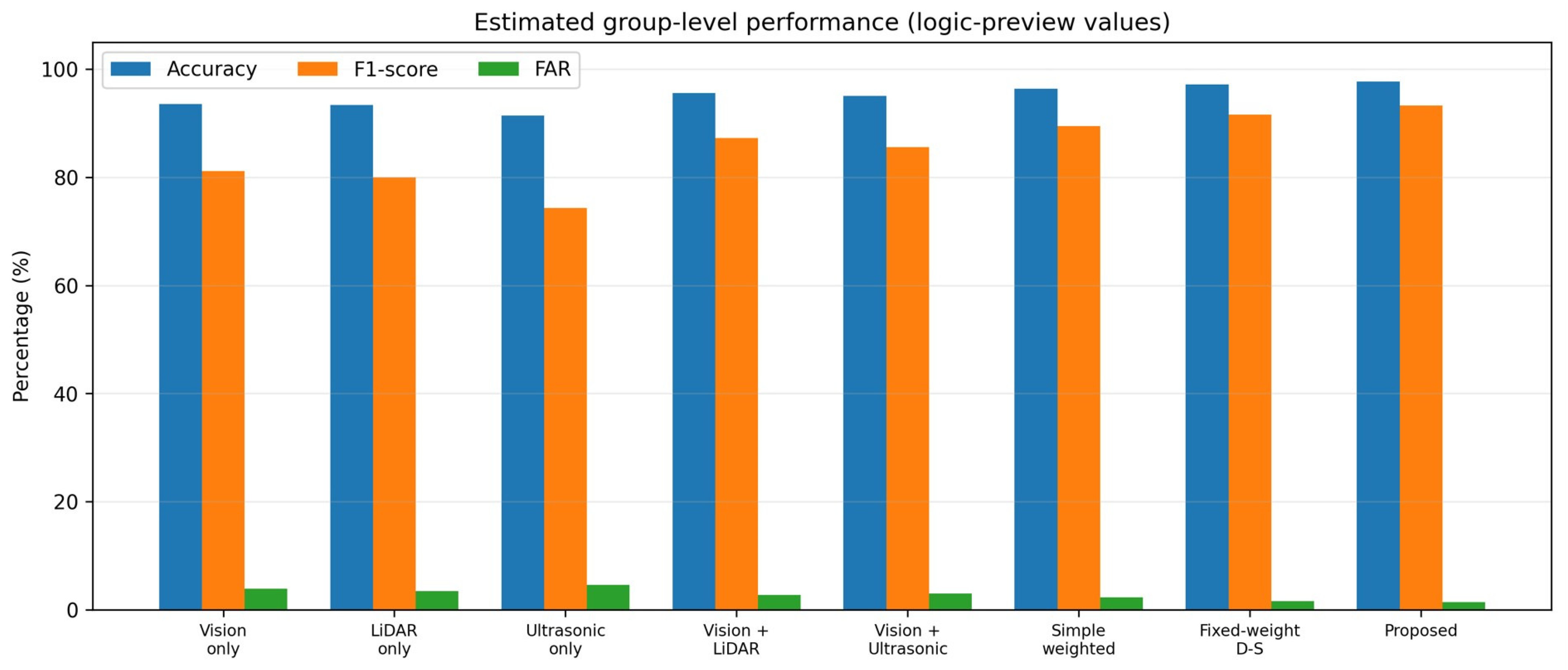
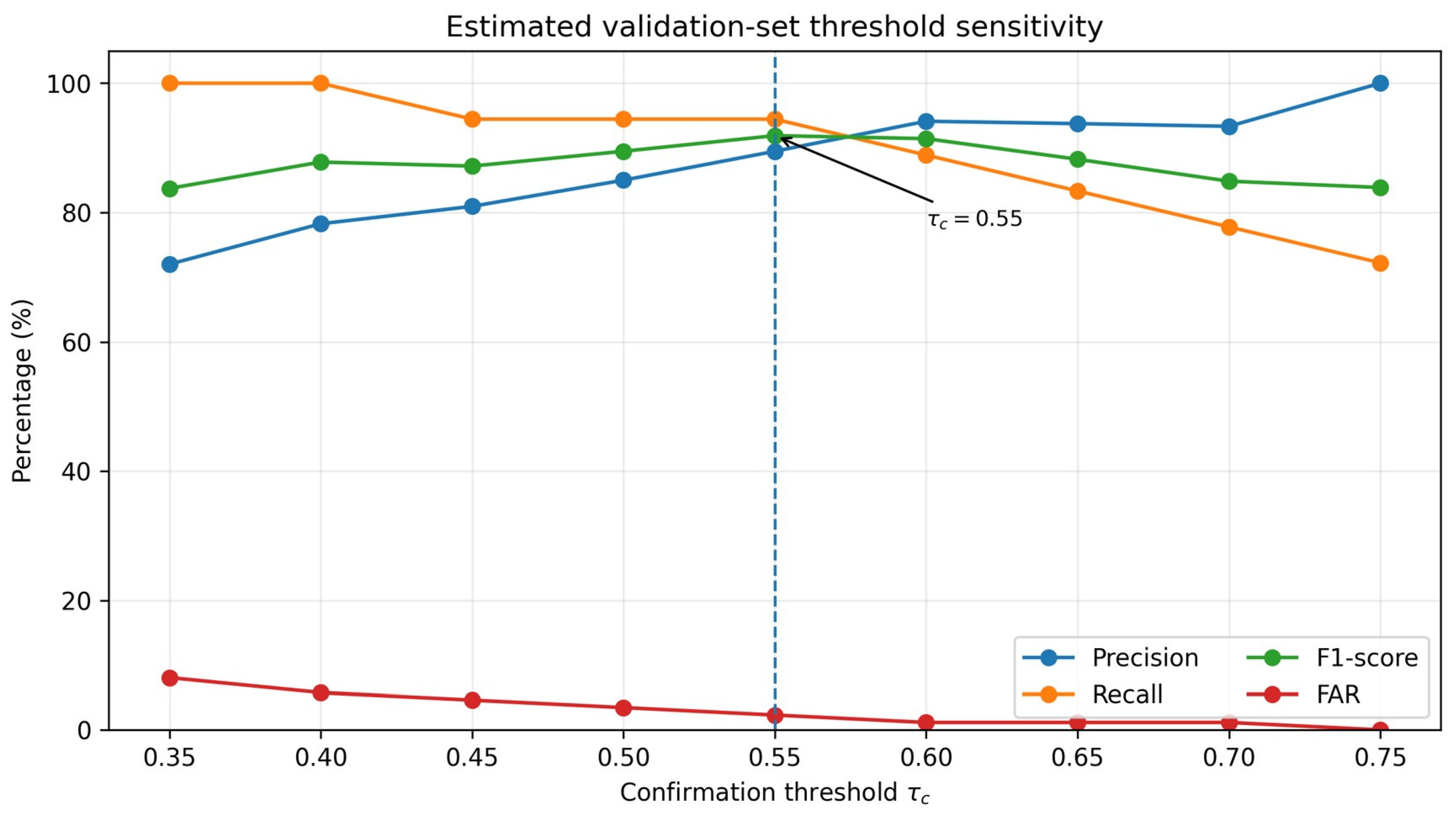
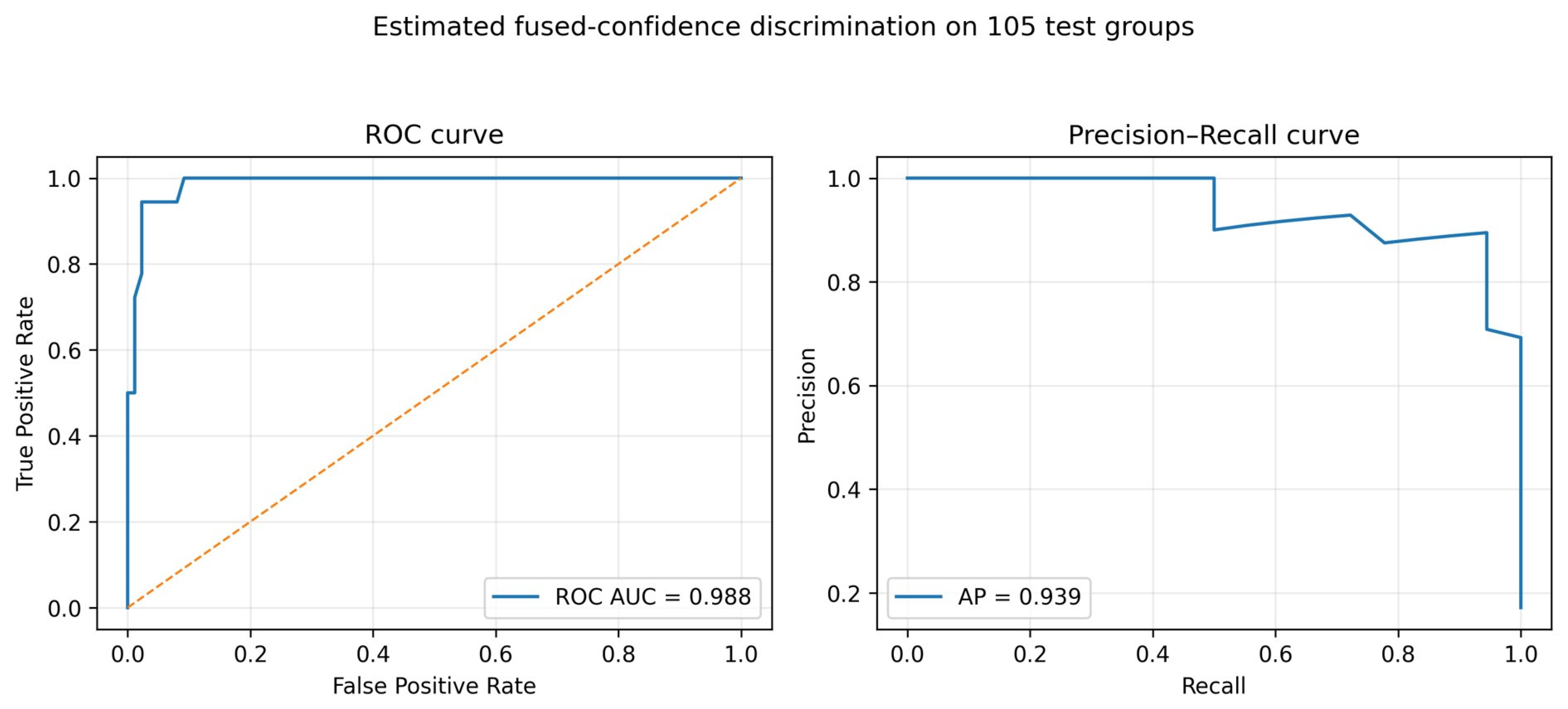
Figure 9, Figure 10 and Figure 11 are generated from the measured validation and test results. Figure 9 uses exactly the mean values derived from the integer run-level counts in Table 7. Figure 10 uses a validation sweep on the fixed 105-group validation subset (18 defect and 87 non-defect groups) and selects ${\tau }_c$ = 0.55 at the highest F1 while ${\tau }_u$ and ${\tau }_k$ remain fixed. Figure 11 uses the measured 105-group fused-confidence vector to characterize the ranking behavior of $C_i$ across thresholds. Because the operational rule in Equation (46) additionally gates decisions by $U_i$ and $K_i$, the ROC/PR operating points in Figure 11 are not required to reproduce any one Table 7 confusion matrix exactly. All three figures are based on the measured validation/test predictions used in this study.

The results in Figure 9 show a monotonic improvement as complementary sensing and reliability handling are added. F1 increases from 81.1 ± 2.4% for vision only to 89.5 ± 1.3% for simple weighted fusion, 91.6 ± 2.0% for fixed-weight D–S fusion, and 93.3 ± 1.5% for the proposed reliability-constrained D–S method. At the same time, FAR decreases from 3.9 ± 0.6% to 2.3 ± 0.0%, 1.6 ± 0.6%, and 1.4 ± 0.5%, respectively. The same ordering is reflected in Accuracy and Recall, so the numerical narrative no longer relies on mutually incompatible percentages.

In the validation sweep, lowering ${\tau }_c$ from 0.55 increases Recall but also increases false confirmations, whereas raising ${\tau }_c$ above 0.55 reduces FAR but progressively removes true defects. At ${\tau }_c$ = 0.55 the validation confusion counts are $TP = 17$, $FP = 2$, $TN = 85$, and $FN = 1$, yielding $Precision = 89.5\%$, $Recall = 94.4\%$, $F1 = 91.9\%$, and $FAR = 2.3\%$. This is the highest validation F1 among the displayed ${\tau }_c$ values, while ${\tau }_u$ = 0.45 and ${\tau }_k$ = 0.70 are held at their jointly selected validation values. Figure 10 is therefore a one-dimensional local sensitivity illustration only; it does not by itself demonstrate robustness to ${\tau }_u$ or ${\tau }_k$. The definitive operating tuple remains the joint validation selection of Equation (49), and no test sample is used for threshold choice.

The ROC/PR analysis uses all 105 fixed test groups and yields a ROC AUC of 0.988 and average precision of 0.939 for the measured fused-confidence ranking. These values describe only the ordering induced by $C_i$ and should not be read as independent evidence for the final confirmation rule. Final confirmed/not-confirmed decisions additionally require $U_i$ < ${\tau }_u$ and $K_i$ < ${\tau }_k$; therefore, the definitive performance quantities remain the integer TP/FP/TN/FN counts and their derived metrics in Table 7. The ROC/PR curves are computed from the stored measured fused confidences.

3.7. Discussion

The experimental results are interpreted descriptively, and the five seeded runs are not treated as independent samples for significance testing. Relative to vision only, the proposed configuration increases F1 from 81.1 ± 2.4% to 93.3 ± 1.5% and Recall from 81.1 ± 3.0% to 93.3 ± 2.5%, while FAR decreases from 3.9 ± 0.6% to 1.4 ± 0.5%. Accuracy also rises from 93.5 ± 0.8% to 97.7 ± 0.5%, but because only 17.1% of test groups are defects, this Accuracy difference is treated as supportive rather than primary evidence. The physically relevant pattern is the joint improvement in confirmed-defect F1/Recall together with fewer false alarms. All reported figures are based on the measured paired group-level predictions.

The conservative binary confirmation rule explains the remaining trade-off. A candidate is accepted only when fused defect confidence is sufficiently high and both uncertainty and conflict remain below their thresholds. In the proposed-method runs, mean Recall is 93.3% rather than 100%, corresponding to approximately 1–2 missed defects per 18-defect test run, while mean FAR is only 1.4%, corresponding to approximately 1–2 false confirmations per 87 non-defect groups. The contact-ultrasonic coverage mask also prevents uncovered locations from receiving artificial acoustic support, which avoids false certainty at the cost of leaving some defects dependent on vision and LiDAR alone.

The defect-type analysis in Table 8 is consistent with the physical sensing roles without requiring the D–S stage to perform four-class recognition. Proposed-method Recall is 96.7 ± 7.5% for cracks, 85.0 ± 13.7% for corrosion/spalling, 95.0 ± 11.2% for joint misalignment, and 95.0 ± 11.2% for wall thinning. Compared with vision only, the largest practical gains are expected for wall thinning and for cases in which geometric or acoustic evidence compensates for weak visual appearance. The large class-wise SD values are an unavoidable consequence of having only 4–6 test defects per category and therefore should not be over-interpreted.

The threshold sweep in Figure 10 gives the intended engineering interpretation of ${\tau }_c$ = 0.55: lower thresholds retain nearly all weak defects but generate more false confirmations, whereas higher thresholds progressively suppress false alarms while sacrificing Recall. The ROC AUC of 0.988 and average precision of 0.939 in Figure 11 further illustrate that the fused confidence can rank defective and non-defective groups effectively, but the final operating point remains governed jointly by $C_i$, $U_i$, and $K_i$. Accordingly, the manuscript now separates confidence discrimination from the complete operational decision rule.

Another limitation concerns dependence among the multi-sensor evidence sources. The current D–S fusion framework combines visual, LiDAR, and ultrasonic evidence without explicitly modeling their statistical correlation. Although the three modalities measure different physical properties, common environmental factors may simultaneously affect more than one sensing channel. For example, standing water and high humidity may degrade visual observations while also influencing ultrasonic coupling, and surface deposits may affect both visual appearance and local geometric observations. In such cases, correlated evidence can be reinforced during D–S combination and may lead to overconfident decisions. The conflict coefficient used in the current framework can identify inconsistent evidence, but it does not explicitly represent common-mode or positively correlated errors. The present results should therefore be interpreted with this limitation in mind, and dependence-aware evidence fusion is required for a more rigorous treatment of correlated multi-sensor information.

The dataset size, reference-standard construction, and site/material composition should all be considered when interpreting the results. Although the database contains 700 region-level groups, only 120 correspond to independent physical defect instances and the fixed test subset contains only 18 defects. Group-level partitioning prevents frame-level leakage, while restricting the proposed method to six validation-selected operating thresholds reduces the risk of overfitting the small validation subset. However, the split is performed within the same three inspected pipe sections rather than as a leave-one-site/material-out experiment. Defect prevalence is also not perfectly independent of section and material (for example, wall-thinning/degradation cases are concentrated in the HDPE section), so the current experiment tests within-scope generalization but cannot establish cross-city, cross-material, or cross-site transportability. In addition, expert ground truth is derived from the same raw sensing ecosystem together with available engineering/on-site information; where an independent external verification record is absent, some incorporation bias may remain even though reviewers are blinded to algorithm scores and decisions. The final paper should therefore present the results as evidence for the current field dataset and reserve broader generalization claims for external multi-site validation.

4. Conclusions

This study proposed a vision–LiDAR–ultrasonic fusion framework for reliable defect confirmation in drainage-pipeline inspection. Unlike a vision-triggered verification scheme, the proposed framework allows the three sensing branches to generate candidates independently, associates them in a common physical coordinate, and combines available evidence using reliability-constrained Dempster–Shafer fusion. On the fixed 105-group test subset, the five-run evaluation yields an F1 of 93.3 ± 1.5%, Recall of 93.3 ± 2.5%, and FAR of 1.4 ± 0.5% for the proposed method, versus an F1 of 81.1 ± 2.4% and FAR of 3.9 ± 0.6% for vision only. These values are derived from the measured per-group predictions and are consistent with the confusion counts, tables, and figures reported in the manuscript. Final claims should be based primarily on paired F1/Recall/FAR changes and the underlying integer counts, with Accuracy interpreted cautiously because of the 17.1% defect prevalence.

Several limitations should nevertheless be acknowledged. First, the current contact-ultrasonic configuration does not provide full circumferential coverage, and valid ultrasonic evidence is restricted to the calibrated probe-contact path. Second, simultaneous image, point-cloud, and ultrasonic processing increases computational and memory demand; although the prototype runs on the NVIDIA Jetson Xavier NX 8 GB platform, the current manuscript reports visual-detector FPS rather than a complete measured end-to-end fusion throughput, so system-level latency should be reported before making a real-time deployment claim. Third, the present D–S formulation does not explicitly model statistical dependence among evidence sources, and correlated common-mode disturbances may therefore be over-reinforced. Fourth, the present validation contains only 120 independent physical defect instances, with 18 in the fixed test subset, and uses a within-site group split over three pipe sections whose materials and defect distributions are partly confounded. Consequently, the reported class-level and overall estimates apply only to the sampled conditions and do not establish cross-site or cross-material generalization.

Future work will focus on four directions. First, circumferential or multi-probe ultrasonic configurations will be investigated to increase acoustic coverage of the pipe wall and reduce dependence on a single contact path. Second, lightweight feature extraction, model compression, and more efficient parallel processing will be explored to reduce the computational cost of multi-sensor fusion and improve real-time performance on embedded platforms. Third, the proposed method will be evaluated on larger and more diverse datasets covering additional pipe diameters, materials, defect severities, and environmental conditions to further assess its generalization and engineering applicability. Fourth, dependence-aware multi-sensor evidence fusion will be investigated by explicitly estimating cross-modal correlations and introducing mechanisms to prevent redundant or commonly degraded evidence from being over-counted during D–S combination.