3D CFD Simulation of a H-Darrieus Turbine with Variable Pitch: A Quantitative Vorticity Analysis

Abstract

Vortices and dynamic stall play a critical role in the performance of vertical-axis wind turbines, often leading to significant energy losses. Active and passive control strategies can be employed to delay the dynamic stall, particularly at low tip-speed ratios below 0.5. In this study, three-dimensional Computational Fluid Dynamics simulations of a Darrieus H turbine equipped with a NACA 0018 airfoil are performed using a sinusoidal pitch control method. A vorticity analysis framework is developed to evaluate vortex transport, growth, and detachment, enabling a rigorous assessment approach. The simulations, conducted at 8 m/s wind speed, are validated against experimental data, showing less than 4% deviation. The analysis examines the correlation between vorticity dynamics and turbine performance across both the span and chord of the airfoil. At a tip-speed ratio of 0.5, where dynamic stall is dominant, the pitch control delays flow separation and increases performance by 238%. At a tip-speed ratio of 1.4, performance improves by 57%, although the flow shifts toward a drag-dominated regime in which vortex detachment plays a reduced role. This demonstrates that quantitative vorticity analysis remains effective under variable pitch and can identify stages of the dynamic stall, including imminent vortex separation, offering a basis for optimizing vertical-axis wind turbines.

1. Introduction

The growing global concern regarding climate has driven a notable interest in the use of renewable energy sources due to their clean, inexhaustible, and increasingly cost-effective nature. Globally, over 80% of energy needs are still met through the consumption of fossil fuels [1,2]. This highlights the urgent need to enhance existing technologies to make them more environmentally friendly and to develop innovative solutions to enable a successful transition to renewable and sustainable energy systems.

Wind power has become a highly beneficial renewable energy alternative, mainly because extracting energy via wind turbines is economically viable. This is especially true when combined with other green technologies, like photovoltaic solar systems [3,4]. Furthermore, wind resources present an excellent pathway for driving hydrogen generation. Hydrogen itself has attracted considerable attention owing to its wide range of uses, such as powering vehicles, substituting traditional portable batteries, and supplying domestic energy [5]. Combining these systems leads to hybrid configurations in which the electrical power generated by wind turbines is directly utilized to synthesize hydrogen through either photocatalytic or electrolytic processes [6].

Wind turbines convert the kinetic energy of the wind into mechanical energy and subsequently into electricity [7]. They are commonly classified as horizontal-axis wind turbines (HAWTs) and vertical-axis wind turbines (VAWTs). While HAWTs generally achieve higher efficiencies [8], VAWTs offer several practical advantages, including operation independent of wind direction, compact installation requirements, and easier maintenance due to ground-level placement of key components [9,10].

Despite these advantages, VAWTs are subjected to highly unsteady aerodynamic phenomena, particularly dynamic stall, which involves the formation, growth, transport, and detachment of vortical structures around the blades [11]. These phenomena strongly influence torque production and overall turbine performance. Consequently, Computational Fluid Dynamics (CFD) has become a widely adopted tool for investigating the complex flow behavior of VAWTs and for supporting aerodynamic optimization studies [12,13,14,15,16].

Most CFD investigations reported in the literature have relied on two-dimensional (2D) simulations. For example, a comprehensive review of 2D RANS simulations of Darrieus turbines is presented in [17]. Although these studies have contributed significantly to the understanding of VAWT aerodynamics, they cannot adequately capture inherently three-dimensional flow structures, particularly blade-tip vortices and associated energy losses [18,19,20,21]. Escudero Romero et al. [21] demonstrated that neglecting these effects leads to an overestimation of aerodynamic performance, especially at high tip-speed ratios (TSR). Their work highlighted the necessity of three-dimensional (3D) CFD simulations for obtaining reliable predictions of torque generation and power extraction in VAWTs.

To improve aerodynamic performance and mitigate dynamic stall, several design and control strategies have been proposed. These include blade geometry modifications, pitch-angle variations [22,23,24,25,26,27,28,29,30,31,32,33,34], active and passive flow-control devices, and micro-vortex generators [35,36]. The common objective of these approaches is to delay flow separation, maintain flow attachment over the blade surface, and reduce the adverse effects of large-scale vortex shedding.

Among these strategies, variable-pitch control has received particular attention because it directly modifies the angle of attack experienced by the blades and, consequently, influences vortex development and dynamic stall behavior. Sagharichi et al. [22,23] demonstrated through 2D CFD simulations that harmonic pitch variations can significantly reduce flow separation and improve energy extraction, particularly in low-TSR conditions. Their vorticity analyses showed smaller and less intense vortical structures compared with conventional fixed-pitch configurations. Similar conclusions were later reported by other researchers using 2D numerical models [28,30].

The transition from 2D to 3D CFD analyses has been more limited. Most 3D studies have focused on fixed pitch-angle modifications rather than continuous pitch variation [31,33]. To the best of our knowledge, Elkhoury et al. [34] were among the first researchers to investigate continuous variable-pitch operation using a fully three-dimensional CFD framework. As in previous studies, vortex evolution was primarily evaluated through qualitative analysis of vorticity contours.

Vortex dynamics play a central role in the aerodynamic performance of VAWTs because they govern the onset of dynamic stall and directly affect torque production [37]. Vorticity is therefore a valuable parameter for describing flow-field evolution, turbulence development, vortex interactions, and flow separation processes [38,39,40]. However, several studies have shown that qualitative interpretation of vorticity contours alone may lead to ambiguous conclusions because it relies heavily on visual assessment.

To address this limitation, Acosta et al. [41], from the Chemical Reactor Engineering Centre (CREC) at The University of Western Ontario (UWO), introduced the Vorticity Index (VI) and the Imminent Vortex Separation Condition (IVSC) as quantitative indicators for vortex analysis. While this methodology provided a more objective framework for identifying vortex evolution and impending flow separation, it was restricted to 2D simulations and therefore did not account for blade-tip effects.

To solve this issue and obtain meaningful quantitative interpretations, Escudero Romero, A., et al. [21] introduced a refined approach by segmenting maximum vorticity values into three blade regions: the Leading-Edge Section (LES), the Middle-Edge Section (MES), and the Trailing-Edge Section (TES). These regions were analyzed across various axial planes of the blade, from the mid-plane to the blade tip. By tracking the maximum vorticity evolution in the LES, MES, and TES, these authors identified four characteristic points (A, B, C and D) describing the sequence of vortex development: (A) initial vorticity rise in the MES; (B) peak LES vorticity before stall onset; (C) maximum MES vorticity linked to imminent vortex separation (IVSC) due to vorticity transport/accumulation from the LES; and (D) vortex detachment. This framework revealed clear correlations between torque and LES vorticity across each plane, providing valuable quantitative insights into vortex transport, subsequent vorticity accumulation, and eventual vortex detachment, all of which characterize a dynamic stall phenomenon. For further details, refer to [21].

Building upon these developments, the present work extends the quantitative vorticity analysis framework to vertical-axis wind turbines operating under continuous variable-pitch conditions. The objective is to investigate how pitch-control strategies modify vortex transport mechanisms and how these changes influence dynamic stall behavior and aerodynamic performance. It is shown that 3D quantitative vorticity analysis provides an original and robust methodology for evaluating design and control strategies, particularly under low-TSR and stall-dominated operating conditions where conventional performance indicators alone are insufficient to fully explain turbine behavior.

2. Numerical Methodology

This section outlines the computational framework established to simulate the aerodynamic behavior of the H-Darrieus wind turbine. It details the physical model, computational domains, solver settings, and the sensitivity analyses performed to ensure the accuracy and reliability of the 3D CFD predictions.

2.1. Physical Model

This study examines a three-blade H-Darrieus turbine with a NACA0018 blade configuration. The rotor dimensions and computational domains adopted from Ma Ning et al. (2018) [37] are summarized in

Table 1. Design parameters of the H-Darrieus wind turbine studied [37].

Parameter	Symbol	Value
Rotor Diameter [m]	D	0.8
Blade Airfoil	-	NACA 0018
Chord Length [m]	c	0.2
Rotor Height [m]	H	0.8
Blades Number	N	3
Solidity	σ	0.75

Note: Solidity, $\sigma =\frac{N·c}{D}.$

, with the shaft being excluded from the modeling analysis.

2.2. Computational Domains

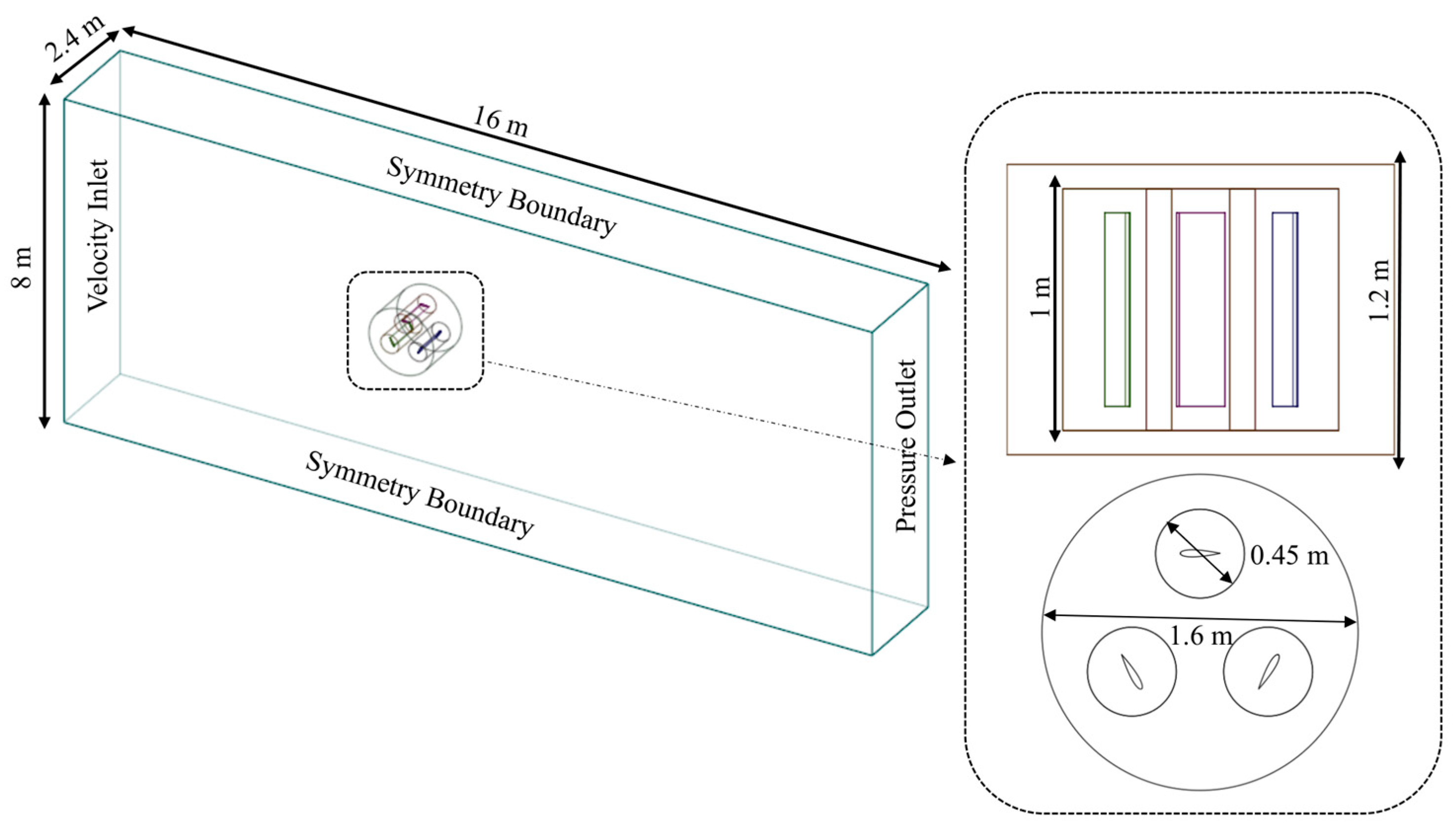
The CFD simulation considers five domains of interest (see Figure 1): (i) a fixed domain (hexahedron control volume), (ii) a rotating domain containing the VAWT rotor, and (iii) three subdomains (one for each blade) used to refine the mesh surrounding the blades and enable variable-pitch motion. The computational domain dimensions are those reported in [37]. They provide a basis for numerical model validation.

The boundary conditions used in the CFD simulations are the following:

(a)

A constant inlet air velocity (${\mathrm{U}}_{\infty }$ = 8 m/s).

(b)

A fixed domain air exit flow, with zero-gauge pressure at the outlet.

(c)

A fixed domain air inlet flow with a 1% turbulence.

(d)

A constant fluid velocity, the same as that of the incoming wind flow (slip wall condition), at the computational upper, lower and lateral domain boundaries.

(e)

A no-slip wall condition at the rotor blade surfaces.

Furthermore, a refined interface between the fixed and rotating domains is used to ensure a smooth transition of information between adjacent cells.

In addition, and to evaluate the soundness of the selected computational domains, a grid sensitivity analysis is performed to evaluate the impact of grid size changes. This procedure ensures appropriate grid selection for the regions near the interface, thereby enabling consistent and accurate data exchange between the simulation domains.

2.3. Solver Settings

The CFD simulations are performed with ANSYS Fluent 21.1. The governing equations include the continuity equation (Equation (1)) and momentum conservation equation (Equation (2)), which are solved using the URANS (Unsteady Reynolds-Averaged Navier–Stokes) Computational Fluid Dynamics method:

$${\displaystyle \frac{\partial }{\partial t}}\rho +𝛻·(\rho \overrightarrow{u})=0$$

(1)

$${\displaystyle \frac{\partial }{\partial t}}\left(\rho \overrightarrow{u}\right)+𝛻·(\rho \overrightarrow{u}\overrightarrow{u})=-𝛻P+𝛻·\tau +\rho \overrightarrow{g}+\overrightarrow{F}$$

(2)

where P represents the static pressure, $𝛻$ is the divergence operator, $\overrightarrow{u}$ is the flow velocity, $\stackrel{̿}{\tau }$ is the stress tensor, and $\overrightarrow{\rho g}$ and $\overrightarrow{F}$ are the gravitational body force and external forces, respectively.

Furthermore, the stress tensor ($\stackrel{̿}{\tau }$) is calculated, as shown in Equation (3):

$$\stackrel{̿}{\tau }=\mu [(𝛻\overrightarrow{u}+{\left(𝛻\overrightarrow{u}\right)}^T)-{\displaystyle \frac{2}{3}}𝛻·\overrightarrow{u}\stackrel{̿}{I}]$$

(3)

where $\mu$ is the molecular viscosity and $\stackrel{̿}{I}$ the unit tensor. One should note that ${\left(𝛻\overrightarrow{u}\right)}^T$ stands for the transpose of the divergence matrix (i.e., rate of expansion) of the flow [18,42].

The numerical framework employs the SST k- approach, which is part of the Reynolds-Averaged Navier–Stokes (RANS) turbulence model category. This specific model is frequently selected for VAWT modeling because it accurately captures both viscous–inviscid fluid interactions and flow separation driven by adverse pressure gradients. Consequently, it represents a highly suitable option for evaluating complex aerodynamic phenomena [18,43].

The transport equations for the turbulent kinetic energy (k) and the specific turbulence dissipation rate ($\omega )$ are Equations (4) and (5), respectively:

$${\displaystyle \frac{\partial }{\partial t}}\left(\rho k\right)+{\displaystyle \frac{\partial }{\partial x_i}}\left(\rho k{u}_i\right)={\displaystyle \frac{\partial }{\partial x_j}}\left({\Gamma }_k{\displaystyle \frac{\partial k}{\partial x_j}}\right)+G_k-Y_k+S_k$$

(4)

$${\displaystyle \frac{\partial }{\partial t}}\left(\rho \omega \right)+{\displaystyle \frac{\partial }{\partial x_i}}\left(\rho \omega u_i\right)={\displaystyle \frac{\partial }{\partial x_j}}\left({\Gamma }_{\omega }{\displaystyle \frac{\partial \omega }{\partial x_j}}\right)+G_{\omega }-Y_{\omega }+S_{\omega }$$

(5)

with $G_k$ representing the turbulence kinetic energy generation and $G_{\omega }$ standing for the generation of $\mathsf{\omega }$. Both variables are defined as in the standard k-ω model. ${\Gamma }_k$ and ${\Gamma }_{\omega }$ denote the effective diffusivities for both k and $\mathsf{\omega }$, respectively. $Y_k$ and $Y_{\omega }$ represent k and $\omega$ dissipations due to turbulence, respectively. $S_k$ and $S_{\omega }$ represent the user-defined source terms.

Regarding the initial conditions at t = 0 s, the computational domains were initialized using a hybrid initialization method to establish a physically consistent flow field, applying the free-stream velocity of 8 m/s and a zero-gauge static pressure prior to the transient calculations.

Table 2. Numerical CFD simulation data.

Parameter	Symbol	Value
Viscous model	SST k-ω	k-ω Shear Stress Transport
Air density	$\mathsf{\rho }$	1.225 kg/$\mathrm{m}$3
Air viscosity	μ	1.79 × $10$−5 Pa·s
Air velocity	$\mathrm{U}$∞	8 m/s
Reynolds number	Re	1.09 × 105
Turbulent intensity		1%
tip-speed ratio	TSR	0.5–1.5
Solver type		Pressure-Based
Coupling method		Coupled
Time discretization		2° of rotation per timestep
Residuals		1 × $10$−4

Note: (a) tip-speed ratio, $\mathrm{TSR}=\frac{\mathsf{\omega }·\mathrm{R}}{{\mathrm{U}}_{\infty }}$, (b) incompressible fluid.

reports the values assigned to the various parameters involved in turbine simulations, such as the fluid physical properties and the solver settings.

2.4. Sensitivity Analysis

To ensure the reliability and accuracy of the numerical results, a sensitivity analysis was conducted to evaluate the impact of both spatial and temporal discretization. This involved testing multiple grid sizes and timesteps.

2.4.1. Grid Size Selection

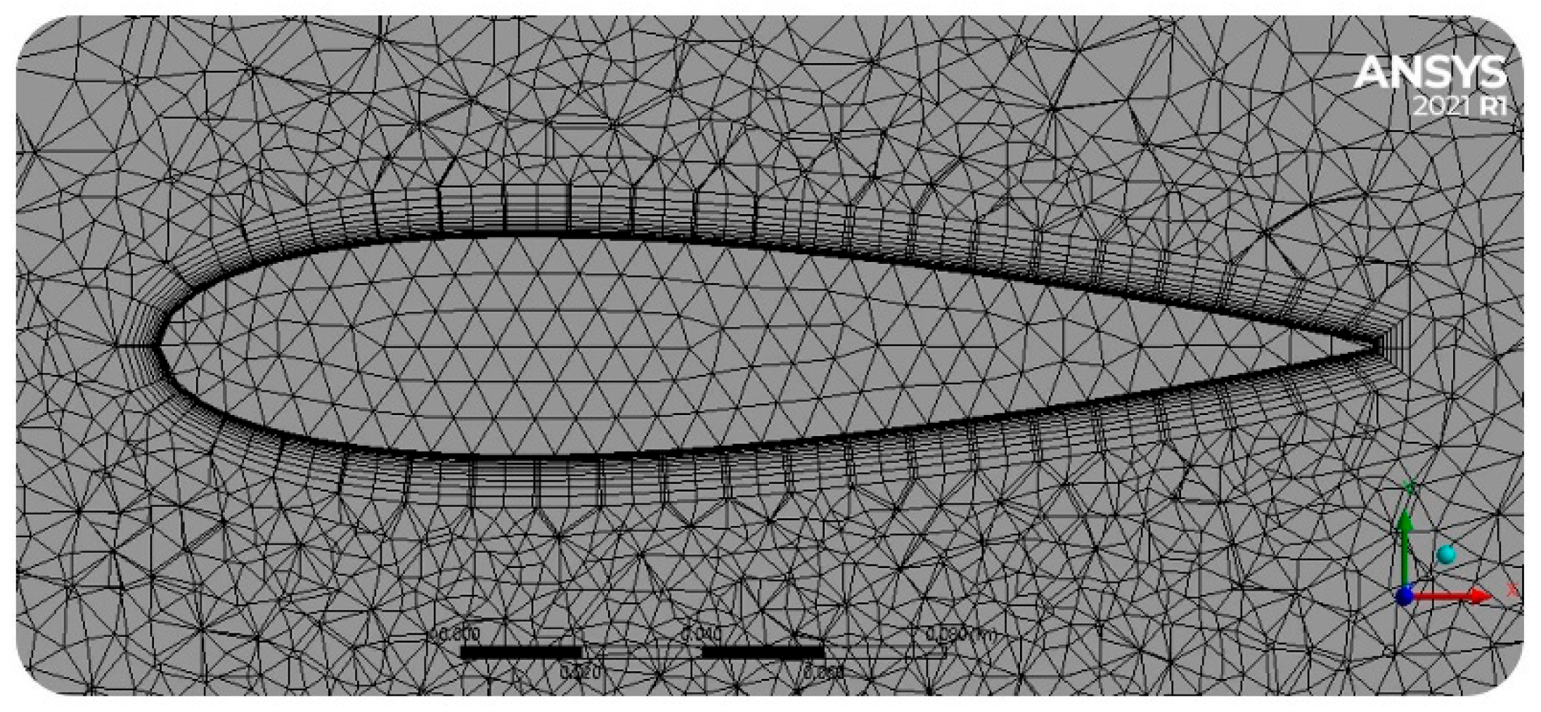
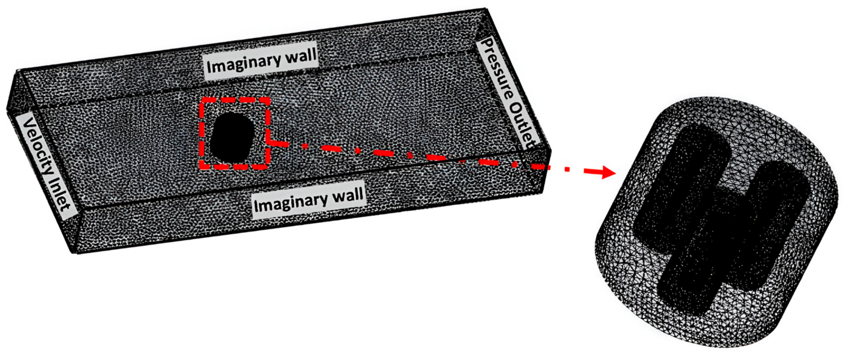
The computational meshes required for the study were generated using the ANSYS 2021 R1 meshing tool. Figure 2 presents the mesh of the airfoil and the surrounding near-airfoil space. Similarly, Figure 3 depicts the mesh within the control volume.

To ensure that the mesh chosen provides sufficient fluid dynamics details near the airfoil–flow interface, it was checked that the commonly recommended Y⁺ parameter values, ranging from 1 to 5, were strictly complied with across all evaluated cases and pitch amplitudes [44]. Under these conditions, the maximum observed skewness is 0.91, slightly below the advised maximum of 0.95, and the minimum orthogonality value is 0.05, slightly below the recommended threshold of 0.1 [41].

Three different mesh sizes were evaluated (see

Table 3. Mesh independence test for TSR = 1.4.

Grid	Total Number of Elements	Cp	Error
Coarse	873,000	0.172	-
Medium	1,461,000	0.189	9%
Fine	2,336,000	0.181	4.4%

) at ${\mathrm{U}}_{\infty }=8 \mathrm{m}/\mathrm{s}$ and TSR = 1.4, after six consecutive rotations of the H-Darrieus wind turbine rotor, with the sixth rotation being considered to calculate C_p values under steady conditions.

The power coefficient (C_p) serves as a primary metric for assessing the overall aerodynamic efficiency and the turbine’s capacity to extract energy from the wind. This parameter is mathematically defined by the following expression:

$$C_p={\displaystyle \frac{\mathit{Turbine} \mathit{power}}{\mathit{Wind} \mathit{power}}}={\displaystyle \frac{T·\omega }{\frac{1}{2}\rho U_{\infty }^3(D H)}}$$

(6)

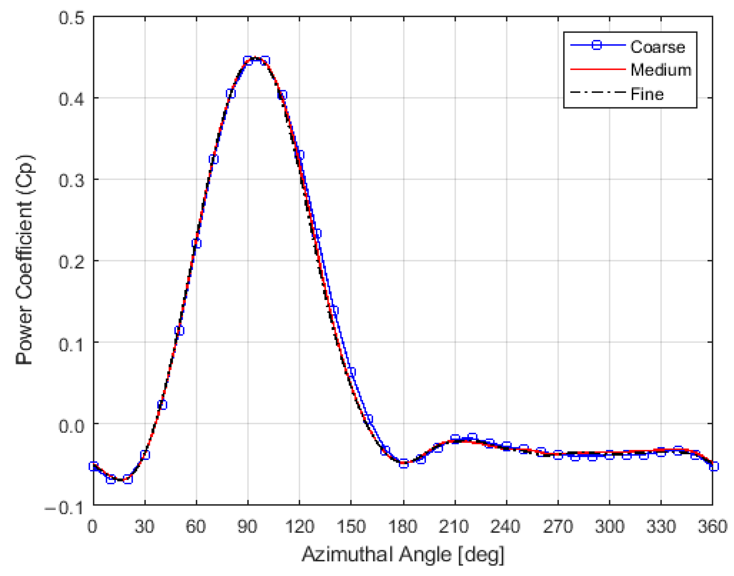
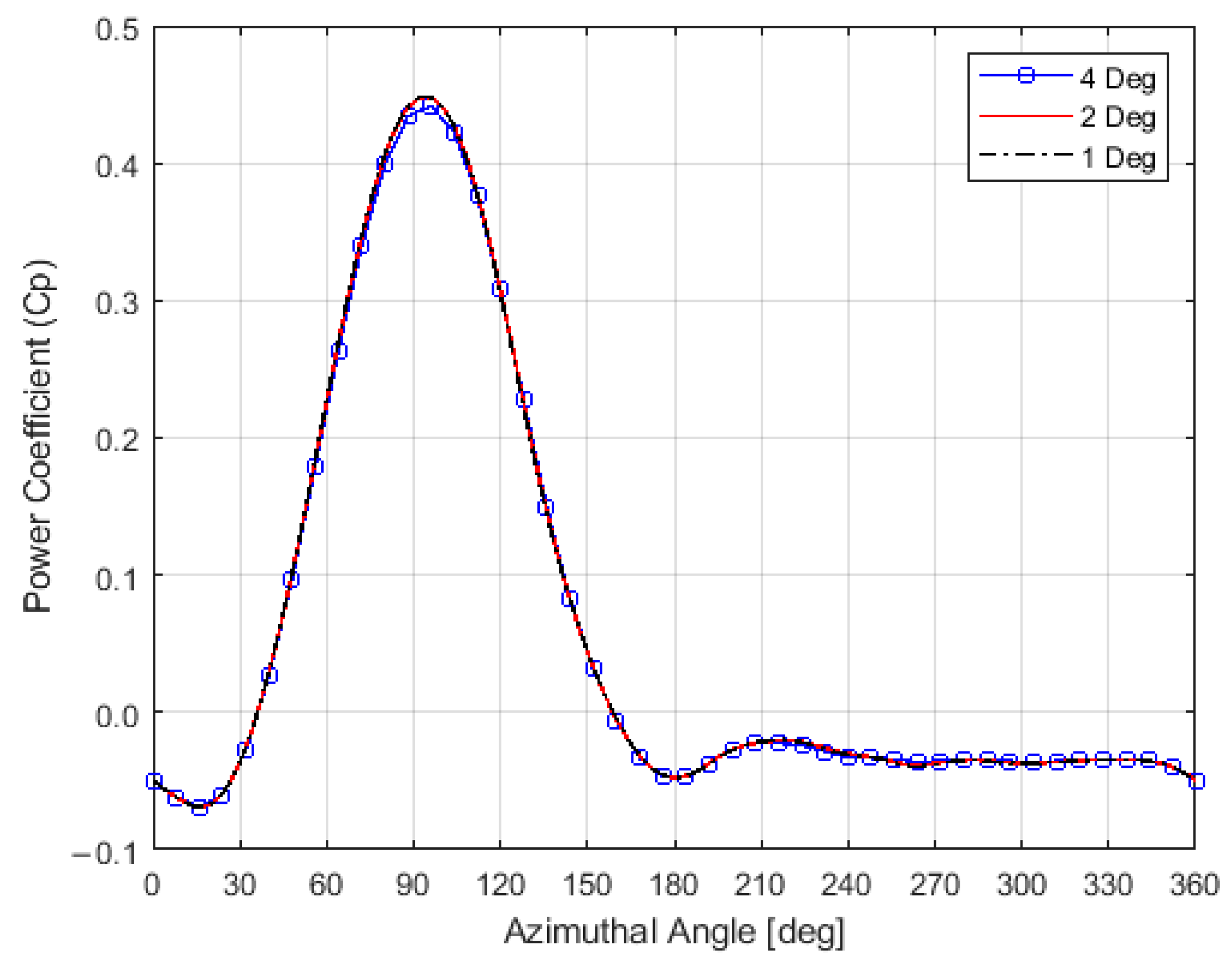
Consequently, grid and temporal resolution independence were verified by tracking the stabilization of the computed C_p as detailed in Table 3. Figure 4 illustrates the C_p trends across the coarse, medium, and fine grids under a constant TSR = 1.4 and a temporal discretization equivalent to a 2° azimuthal increment.

It was observed that all three meshes tested produced close stabilized C_p values. While a coarser mesh would have been optimal to minimize computational time, the finest mesh was selected for all subsequent calculations to ensure the highest possible level of spatial accuracy for the localized vorticity analysis.

2.4.2. Timestep Selection

The timestep size strongly influences unsteady CFD results. Simulations were performed at $U_{\infty }=$ 8 m/s and at TSR = 1.4, using the fine mesh while testing three timesteps of 0.0025 s $(∆\mathsf{\alpha }=4°$), 0.0013 s $(∆\mathsf{\alpha }=2°$), and 0.0006 s $(∆\mathsf{\alpha }=1$), during six consecutive rotations of the H-Darrieus wind turbine. The method considered was found to be reliable to identify the most appropriate timestep required and to calculate C_p values, while minimizing computational time [41]. It is important to note that this approach is in agreement with the findings reported by Ma Ning et al. [37].

Figure 5 reports the C_p values obtained for various azimuthal angles. Figure 5 shows that an angular step of 2° and a fine mesh are adequate to balance computational efficiency and accuracy.

2.5. Comparison with Experimental Data

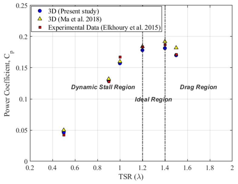
Figure 6 compares C_p values at various TSRs, using the experimental data obtained by Elkhoury et al. [34], as well as the 3D simulation results acquired by Ma Ning et al. [37] and the outcomes obtained in the present study. C_p values acquired using the 3D models are very similar to those obtained with the experimental data from Elkhoury et al. [34]. Specifically, the Mean Absolute Percentage Error (MAPE) between the numerical predictions and the experimental measurements across the evaluated TSR range is 3.68%. Thus, one can conclude that the consistency of 3D model predictions, with experimental data in the full range of the TSRs, is an excellent indicator that the 3D proposed model is suitable for CFD VAWT analysis.

Furthermore, on the basis of the results reported in Figure 6, and as a reference for the upcoming result discussion, three characteristic TSR operating regions, as identified by Sagharichi [22], are considered:

(i)

Dynamic stall region (0.5 < TSR < 1.2);

(ii)

Optimum operating range (1.2 < TSR < 1.4);

(iii)

Drag region, where viscous and friction effects dominate (TSR > 1.4).

2.6. Effect of Angle of Attack (α) on C_p

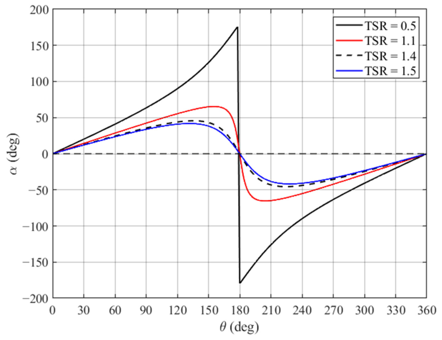
When comparing the C_p values for different TSR conditions as shown in Figure 6, it is apparent that TSR = 1.4 yields better power extraction relative to TSR = 0.5. This difference can be attributed to the higher geometrical angles of attack ($\mathsf{\alpha }$) experienced by the blades at TSR = 0.5 (as shown in Figure 7), where strong dynamic stall phenomena govern blade aerodynamics.

Regarding the angle of attack ($\mathsf{\alpha }$), it can be calculated according to Equation (7), following [41]:

$$\alpha =arctan\left(\mathit{sin}\right(\theta )/(\mathit{cos}\left(\theta \right)+\mathit{TSR}\left)\right)$$

(7)

Figure 7 shows that at low TSR, the blades reach large absolute angles of attack, approaching 200°. In contrast, at TSR = 1.5, the maximum $\mathsf{\alpha }$ remains below 50°, highlighting the significant influence of TSR on aerodynamic loading.

2.7. Variable Pitch Angle

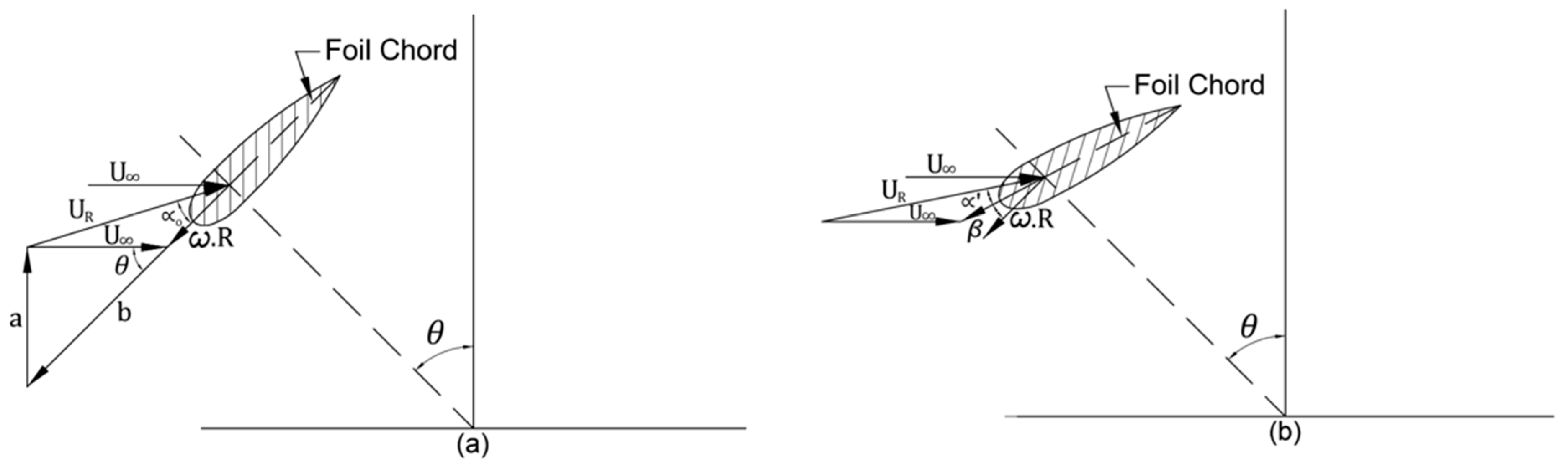
Figure 8 aims to visually facilitate the understanding of the various forces and characteristic angles acting on a VAWT blade. Symbols assigned in Figure 8 are defined as follows: θ = azimuthal angle, $\alpha$ = geometrical angle of attack, $\omega$ = angular velocity, and $\beta$ = pitch angle).

One can notice in Figure 8b that increasing the β pitch angle reduces the angle of attack ($\alpha$), leading under low TSRs to higher power extraction with reduced dynamic stall. However, it can also be noticed that excessively lowering the angle of attack in high-TSR conditions could have a negative impact, as viscous and frictional effects become more significant [22,29]. These matters are further described in Section 3.1, where the overall C_p values for TSR 0.5 and 1.4 are reviewed for a VAWT operated with different variable β pitch angle amplitudes.

In this sense, and to corroborate the statement above, an active variation in the geometrical angle of attack through pitch angle variation is introduced in this section at the lowest and highest TSR-C_p operating points (i.e., TSRs of 0.5 and 1.4). This is achieved by implementing a User-Defined Function (UDF) in which the pitch angle is computed according to Equation (8) [22].

$$\beta =A_{max}·sin\left(\theta \right)$$

(8)

where $\beta$ is the instantaneous pitch angle applied to each blade, ${\mathrm{A}}_{\mathrm{m}\mathrm{a}\mathrm{x}}$ is the maximum local amplitude that will be reached by the airfoil (i.e., referred to the airfoil axis), and $\theta$ is the blade azimuthal position. The resulting geometrical angle of attack ${\alpha }^{\prime }$ is then calculated with Equation (9):

$${\alpha }^{\prime }=\alpha -\beta$$

(9)

where $\alpha$ is the unmodified angle of attack at that same azimuthal position when no pitch angle variation is applied as described in Figure 8a.

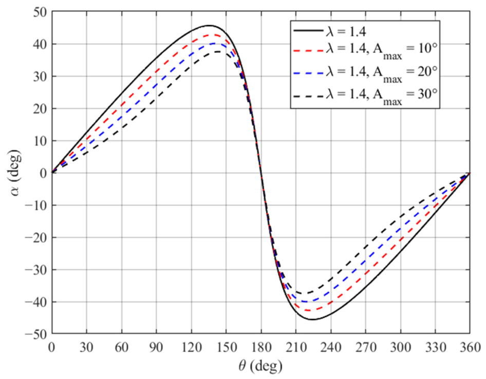
It is important to note that the motion applied to the airfoil (Equation (8)) follows a specific pattern: (a) it moves clockwise from 0 to π/2, (b) then counterclockwise from π/2 to π, (c) counterclockwise again from π to 3π/2, and (d) finally clockwise from 3π/2 to 2π. This movement keeps the instantaneous angle of attack closer to the stall angle, thereby enhancing torque [45] and generating smoother overall motion patterns. One should note, however, that as described by Equation (9) and Figure 9, the introduction of the pitch variations reduces the effective angle of attack in β degrees relative to a fixed-pitch configuration.

Figure 9 shows the modified angle-of-attack profiles at TSR = 1.4 for maximum amplitudes of 10°, 20°, and 30°. As expected from Equation (9), higher pitch amplitude results in lower α′ effective angles of attack.

2.8. Instantaneous Torque and Vorticity Evaluation Methodology

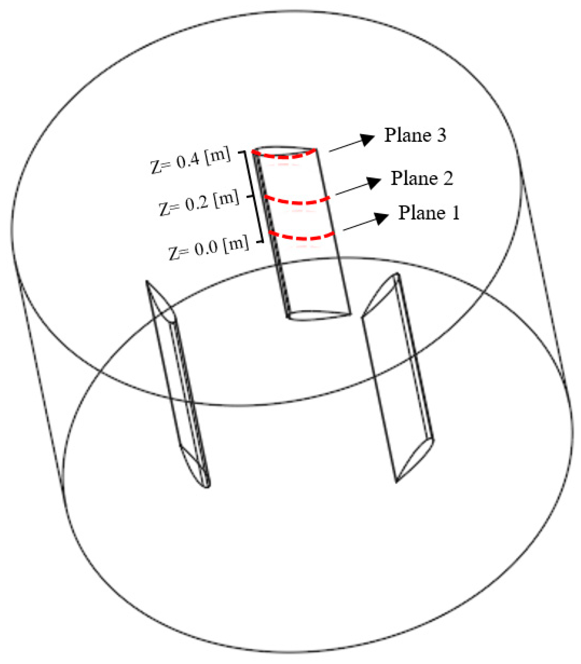
The methodology employed in this study to evaluate instantaneous torque follows the approach presented in our previous work [21]. Half of the blade span was discretized into three cross-sectional planes, each separated by 0.2 m, as illustrated in Figure 10. This discretization assumes axial flow symmetry about the airfoil, whereby the aerodynamic behavior of the upper half of the blade is considered representative of the lower half. Furthermore, Blade 1 is designated as the reference blade for all subsequent analyses.

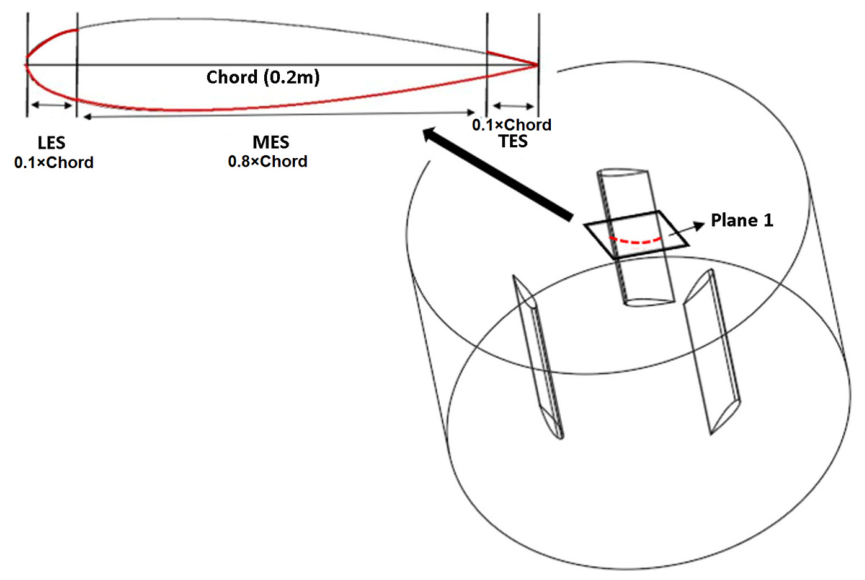
As in our previous work [21], three spanwise sections were examined to assess the influence of vorticity on turbine performance: the Leading-Edge Section (LES), Mid-Inner-Edge Section (MES), and Trailing-Edge Section (TES), shown in Figure 11. These sections were analyzed to determine the maximum vorticity at each location.

The objective of this methodology is to determine whether the characteristic points (A, B, C, and D) identified in [21] and described in the introductory section are still present under the conditions analyzed. Specifically, we identify the Imminent Vortex Separation Condition (IVSC), which is quantitatively defined as the precise azimuthal position at which the maximum vorticity magnitude is reached within the Mid-Edge Section (MES), designated as Point C in this framework. Furthermore, the study evaluates how the occurrence and behavior of these points can be used to quantitatively assess the beneficial or detrimental influence of vortices as the pitch angle varies across different tip-speed ratio (TSR) conditions.

Additionally, given the limited number of three-dimensional CFD studies investigating variable-pitch-angle strategies, instantaneous torque analysis—following the approach outlined in [12,13,21]—is employed to assess the effect of an active β variable-pitch strategy on torque, with particular emphasis on the blade tip region.

3. Results

This section presents the outcomes of the 3D CFD simulations. The analysis first evaluates the impact of variable pitch amplitude on the overall power coefficient, followed by a detailed assessment of instantaneous torque distribution and quantitative vorticity dynamics across different blade planes.

3.1. Effect of Pitch Amplitude on the Power Coefficient (C_p)

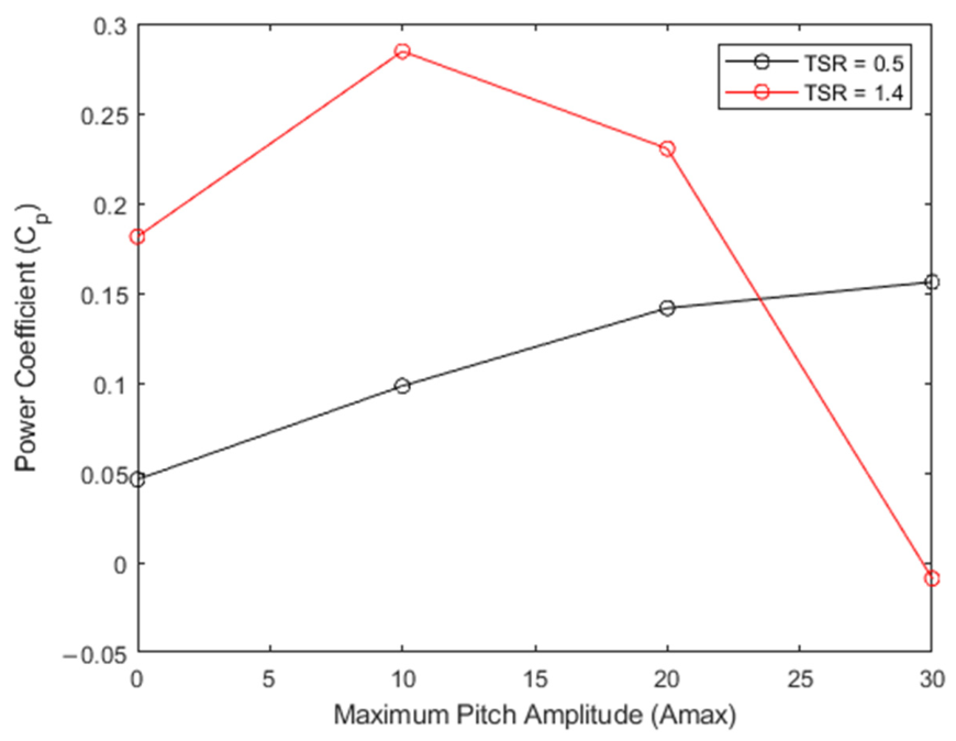
Figure 12 presents the results of the β variable-pitch strategy, implemented using the sinusoidal function defined in Equation (8), for two operating conditions corresponding to the lowest and highest aerodynamic performance (TSR = 0.5 and 1.4). Three A_max maximum local pitch amplitudes (10°, 20°, and 30°) are evaluated, along with the fixed-pitch case (0°), which serves as the baseline for comparison.

Two distinct behaviors are observed depending on the tip-speed ratio (TSR) and the selected A_max maximum pitch amplitude (see

Table 4. Power coefficient (C_p) and its percentage variation relative to fixed pitch for different maximum pitch amplitudes at TSR = 0.5 and TSR = 1.4.

	$\mathit{M}\mathit{a}\mathit{x}\mathit{i}\mathit{m}\mathit{u}\mathit{m} \mathit{P}\mathit{i}\mathit{t}\mathit{c}\mathit{h} \mathit{A}\mathit{m}\mathit{p}\mathit{l}\mathit{i}\mathit{t}\mathit{u}\mathit{d}\mathit{e} \left({\mathit{A}}_{\mathit{m}\mathit{a}\mathit{x}}\right)$ $\mathit{D}\mathit{e}\mathit{g}\mathit{r}\mathit{e}\mathit{e}\mathit{s} (°)$	${\mathit{C}}_{\mathit{p}}$	$\%∆{\mathit{C}}_{\mathit{p}}$
$TSR=0.5$	0	0.05	-
	10	0.10	112.5
	20	0.14	206.2
	30	0.16	237.7
$TSR=1.4$	0	0.18	-
	10	0.28	56.9
	20	0.23	27.0
	30	−0.01	−104.9

and Figure 12).

(a)

TSR = 0.5. This regime is characterized by dynamic stall. Increasing the maximum pitch amplitude from 0° to 30° results in a monotonic increase in the power coefficient (C_p). This improvement is attributed to a reduction in the geometric angle of attack (Figure 8), which delays the onset of dynamic stall and prolongs the duration of attached flow, thereby enhancing torque generation.

(b)

TSR = 1.4. At this TSR, corresponding to near-optimal operation under fixed-pitch conditions, a small increase in pitch amplitude initially improves performance. However, beyond a threshold value, further increases shift the blade away from its optimal angle of attack, leading to a regime increasingly dominated by drag and viscous effects. Consequently, performance deteriorates, with the most extreme case observed at a 30° amplitude, where C_p is reduced to near zero relative to the fixed-pitch case, indicating a near-complete loss of power generation.

Similar trends have been reported in the technical literature, where increasing pitch amplitude enhances the power coefficient up to a certain limit, beyond which performance declines due to elevated drag forces [22].

3.2. Effect of Pitch Amplitude on Instantaneous Torque Analysis

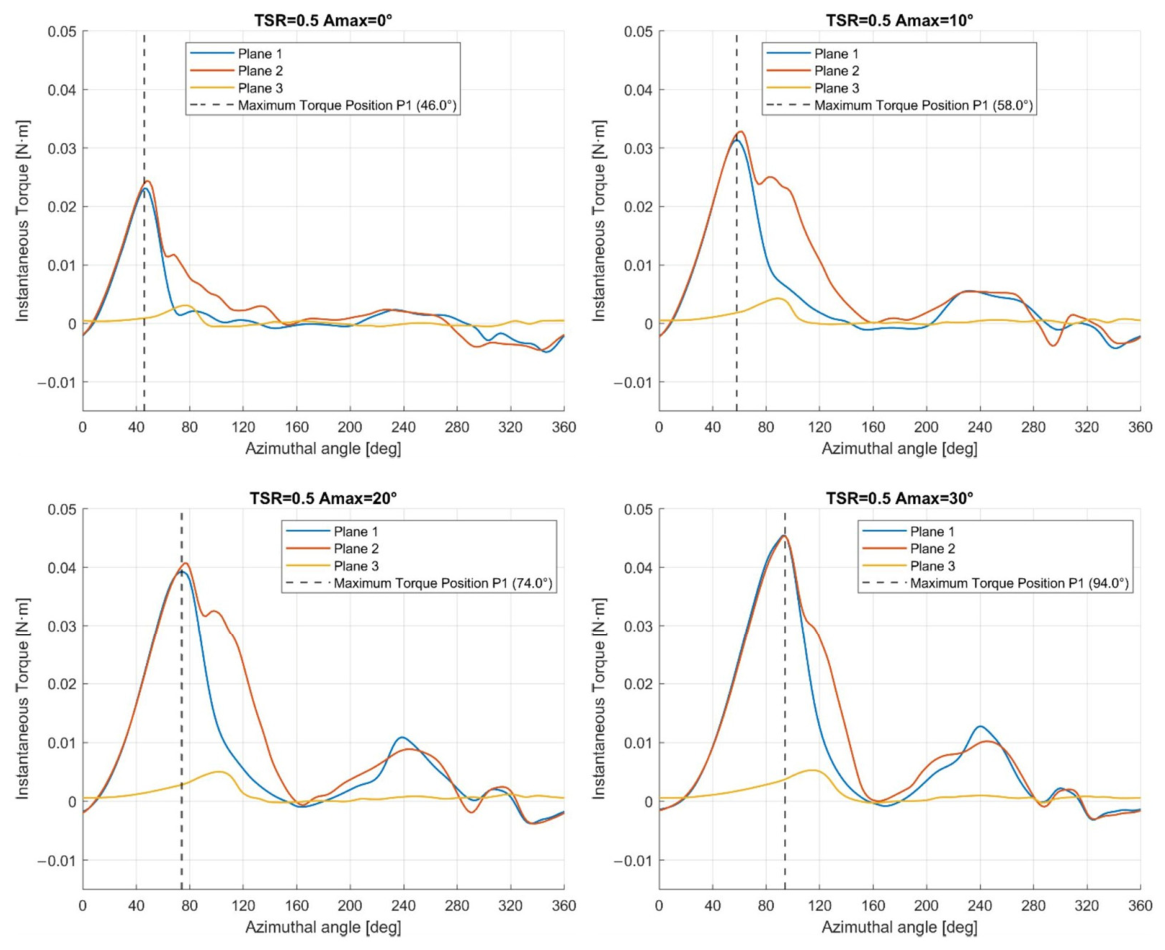
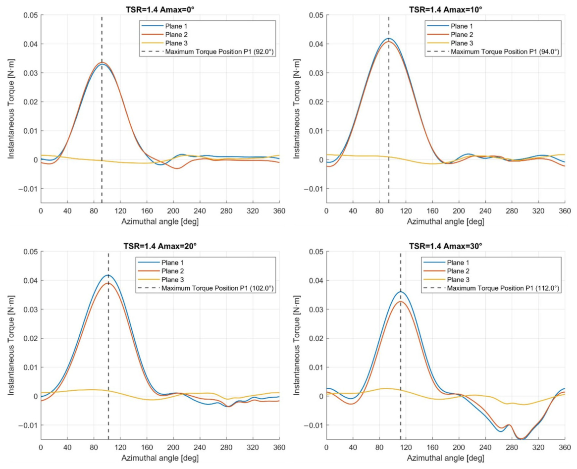
Figure 13 and Figure 14 display the instantaneous torque profiles for the two TSRs at different planes conditions considered in this work (as shown in Figure 10).

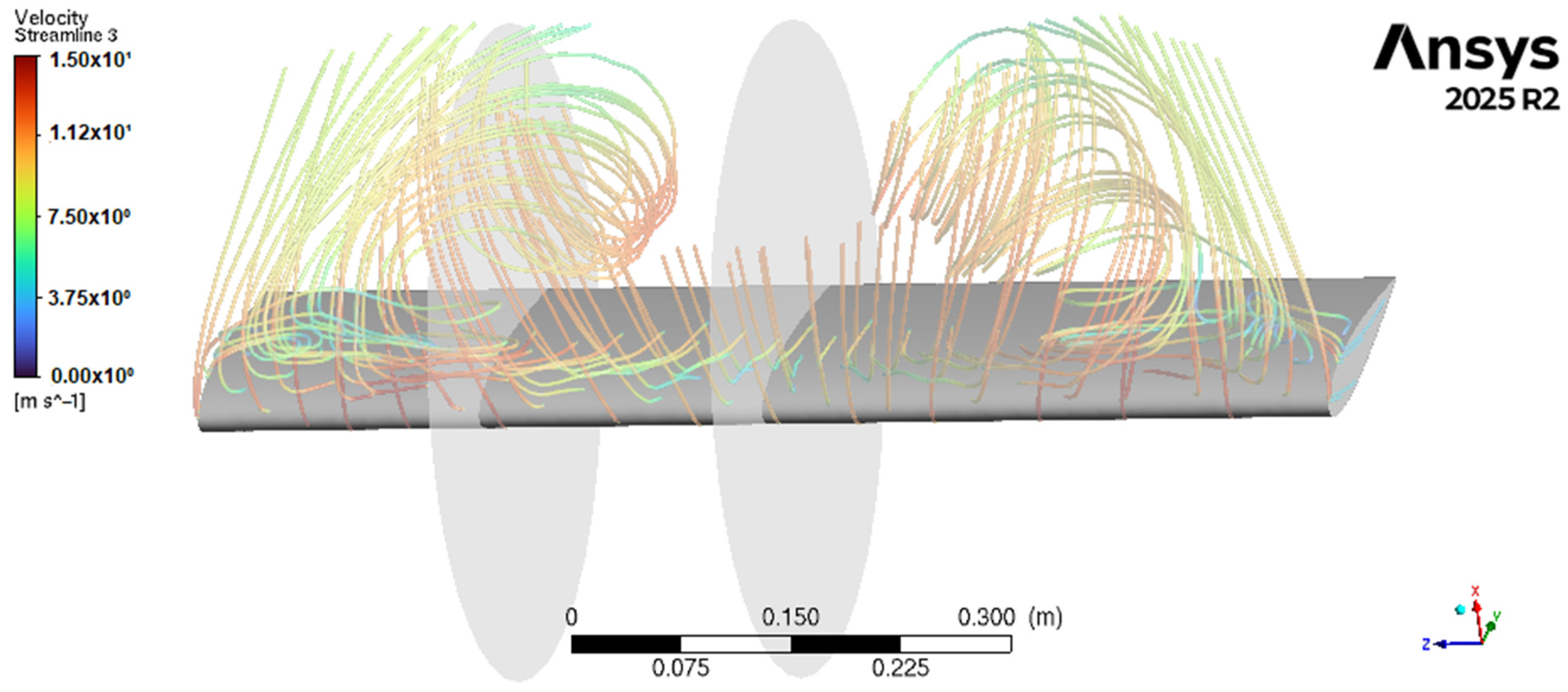
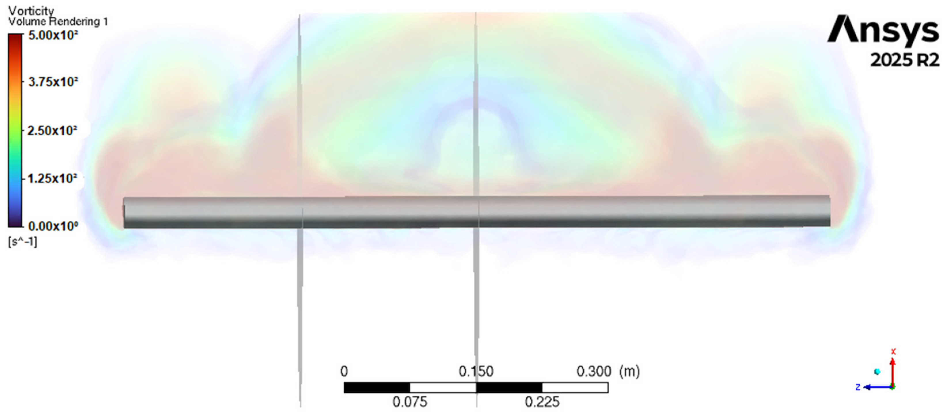
Figure 13 (TSR-0.5) reveals a consistent trend in which the instantaneous torque at Plane 2 exceeds that at Plane 1 for a TSR of 0.5. Although the mid-span location (Plane 1) would be expected to yield the highest torque due to reduced exposure to tip vortices, previous studies [21,40] attribute this higher torque in Plane 2, due to flow reattachment induced by these vortices. This reattachment promotes the persistence of a leading-edge vortex (LEV), particularly under deep dynamic stall conditions, thereby enhancing energy extraction [46]. In contrast, Plane 3, corresponding to the blade tip, displays a significant reduction in torque, highlighting the limitations of two-dimensional models and underscoring the importance of three-dimensional simulations. This tip-vortex-induced flow reattachment is visually corroborated by velocity streamlines and volume-rendered vorticity for a representative case, as provided in Appendix A

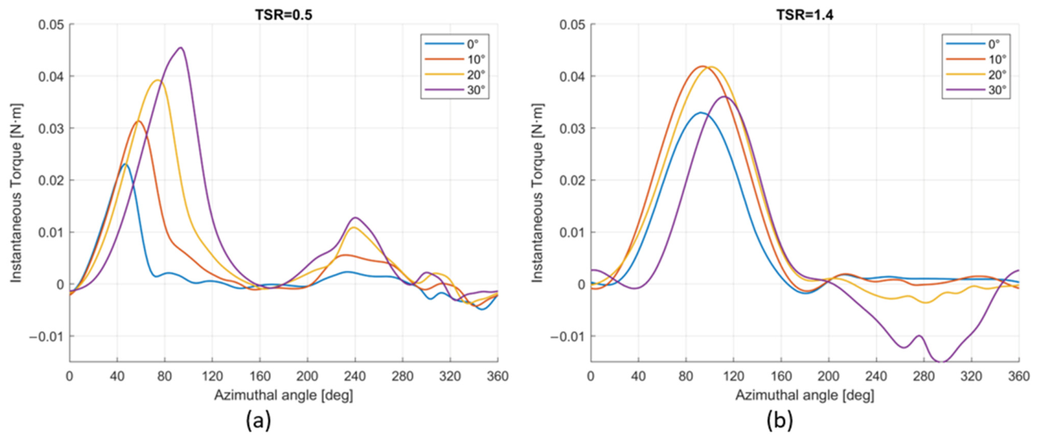
Furthermore, a consistent increase in instantaneous torque at Planes 1 and 2 is also observed with increasing A_max maximum pitch amplitude, with this being consistent with the enhancement in the power coefficient (C_p) discussed earlier. Additionally, the azimuthal position corresponding to the maximum instantaneous torque shifts towards higher azimuthal angles, indicating a displacement in the onset of flow separation and, consequently, the development of the dynamic stall vortex, as further discussed in Section 3.3.

Figure 14 (TSR = 1.4) further supports these observations. During the first half of the rotation (0–180°), the instantaneous torque increases for A_max maximum pitch amplitudes of 0°, 10°, and 20°, but decreases significantly at 30°. In the second half of the cycle (180–360°), the torque becomes slightly negative, which contributes to the difference in C_p between the 10° and 20° cases. At 30°, a substantial reduction in instantaneous torque is observed throughout the rotation, consistent with the near-complete reduction in C_p relative to the fixed-pitch case. Notably, the azimuthal position of maximum torque remains nearly unchanged for 0°, 10°, and 20°, likely due to the relatively low angles of attack associated with TSR = 1.4.

The obtained results provide further insight as reported in Figure 15a,b, regarding the instantaneous torque at Plane 1 for TSR = 0.5 and TSR = 1.4, respectively. The results compare the fixed-pitch case with variable maximum pitch amplitudes of 10°, 20°, and 30°, illustrating how torque evolution varies with both A_max and airfoil operating conditions.

It is worth noting that similar trends regarding instantaneous torque and the effects of variable pitch have been reported previously (e.g., [22,23,28,29,30]). However, those studies were primarily based on two-dimensional models, which cannot capture spanwise variations or inherently three-dimensional flow phenomena such as tip vortices and flow reattachment. The present work extends these earlier findings by providing a quantitative three-dimensional analysis across multiple spanwise planes and a range of pitch amplitudes (A_max). This comprehensive approach enables a deeper understanding of the governing aerodynamic mechanisms, including spanwise torque distribution, the shift in flow separation and dynamic stall onset with pitch variation, all of which are critical for turbine performance optimization.

3.3. Quantitative Vorticity Analysis

Vorticity plays a central role in flow separation, vortex formation, and the dynamic stall process, all of which strongly influence torque production and overall efficiency. A key contribution of the present work is the transition from qualitative vortex visualization to quantitative vortex diagnostics. Rather than relying exclusively on visual interpretation of vorticity contour plots, the proposed methodology provides a quantitative framework for identifying vortex development, vorticity transport, accumulation, and detachment through the analysis of characteristic vorticity levels at the LES, MES, and TES locations. Furthermore, the introduction of the Imminent Vortex Separation Condition (IVSC) enables the identification of the onset of vortex detachment. This framework provides objective indicators of vortex transport, accumulation, and detachment, establishing a direct link between vortex dynamics and torque production. As a result, the aerodynamic effects of variable-pitch operation can be quantified and compared using physically meaningful metrics rather than solely qualitative flow visualizations.

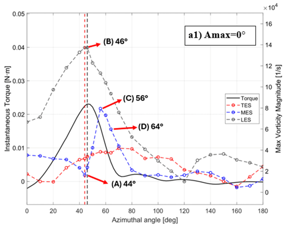
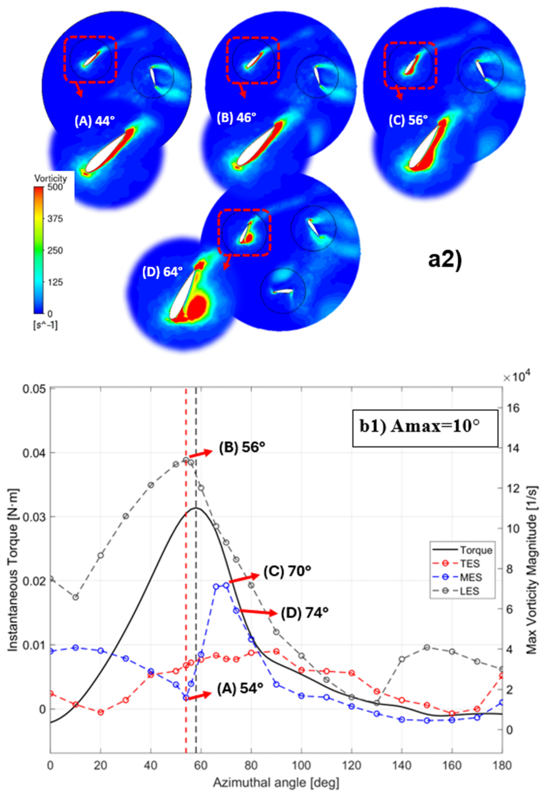
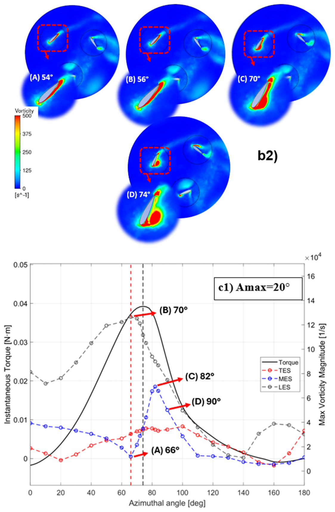
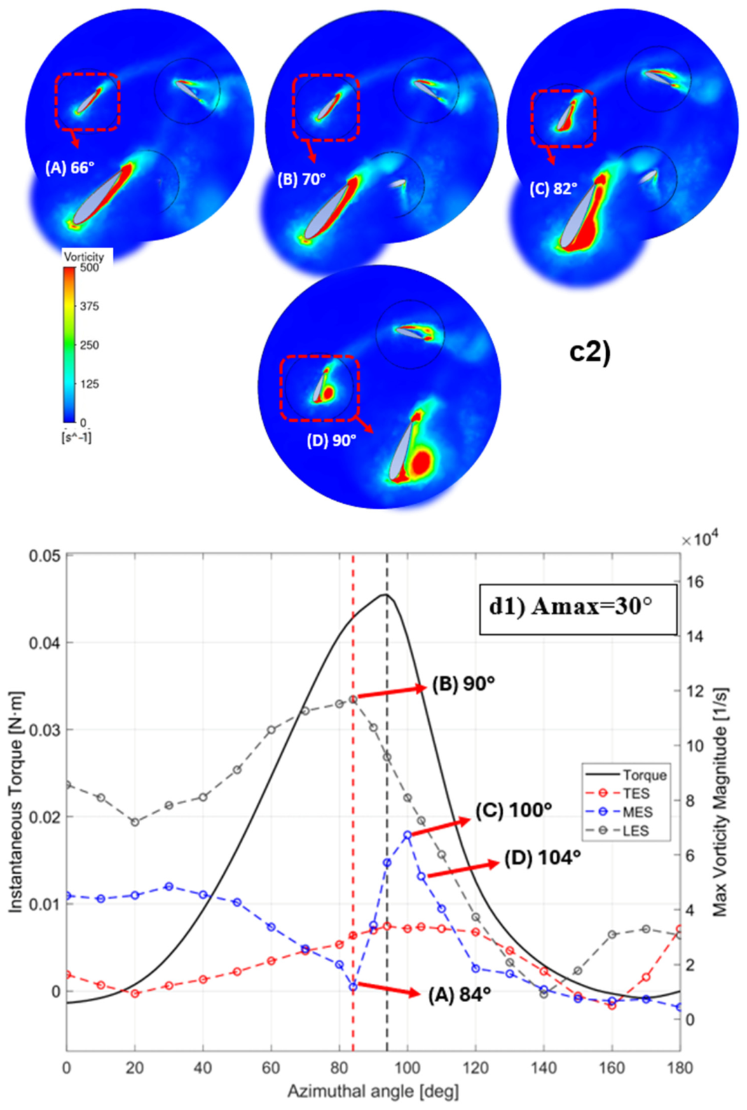
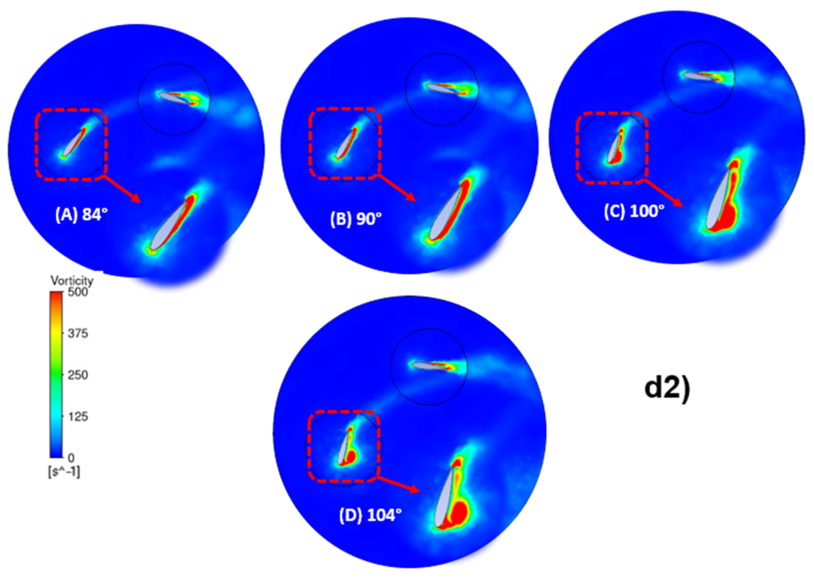
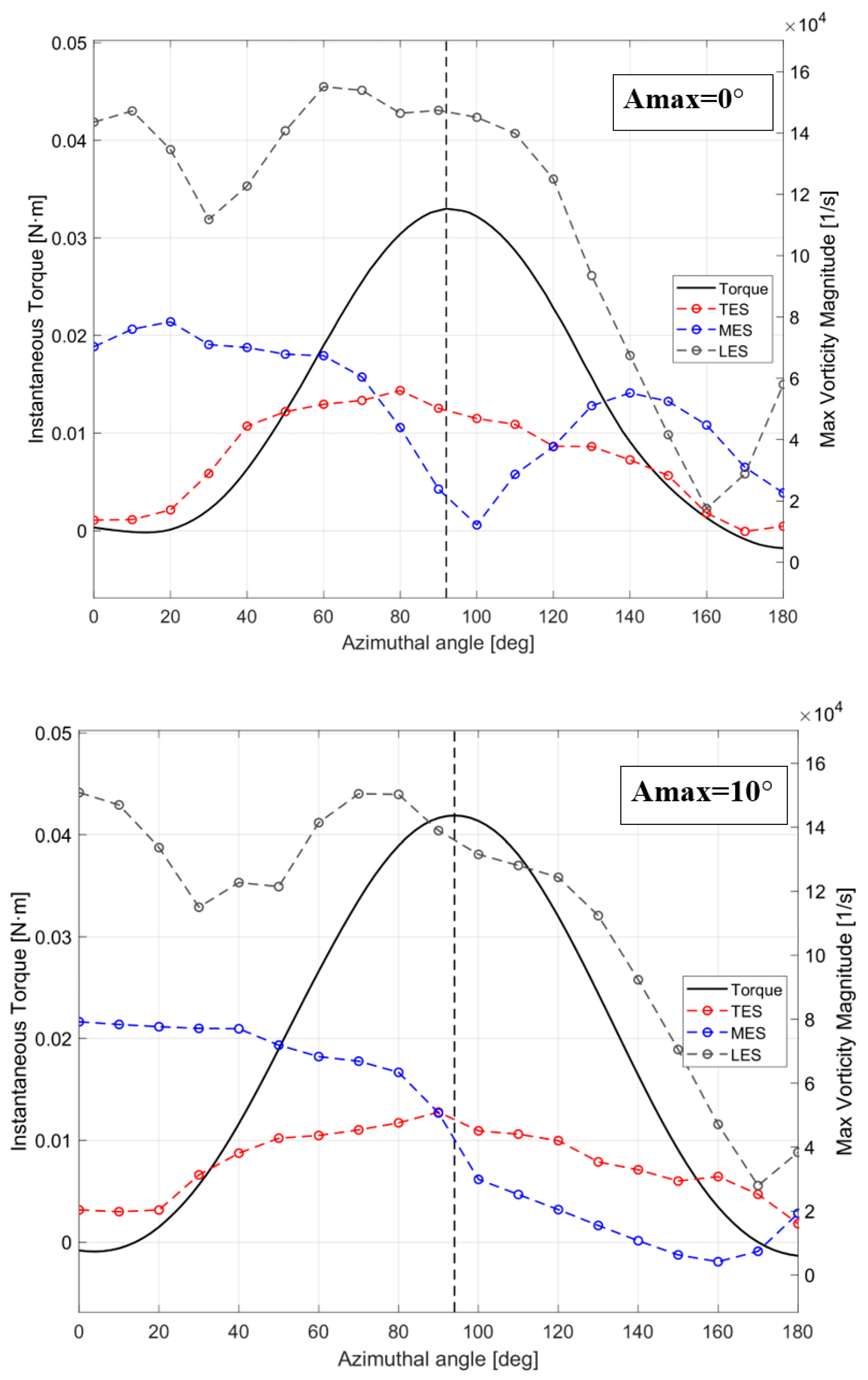
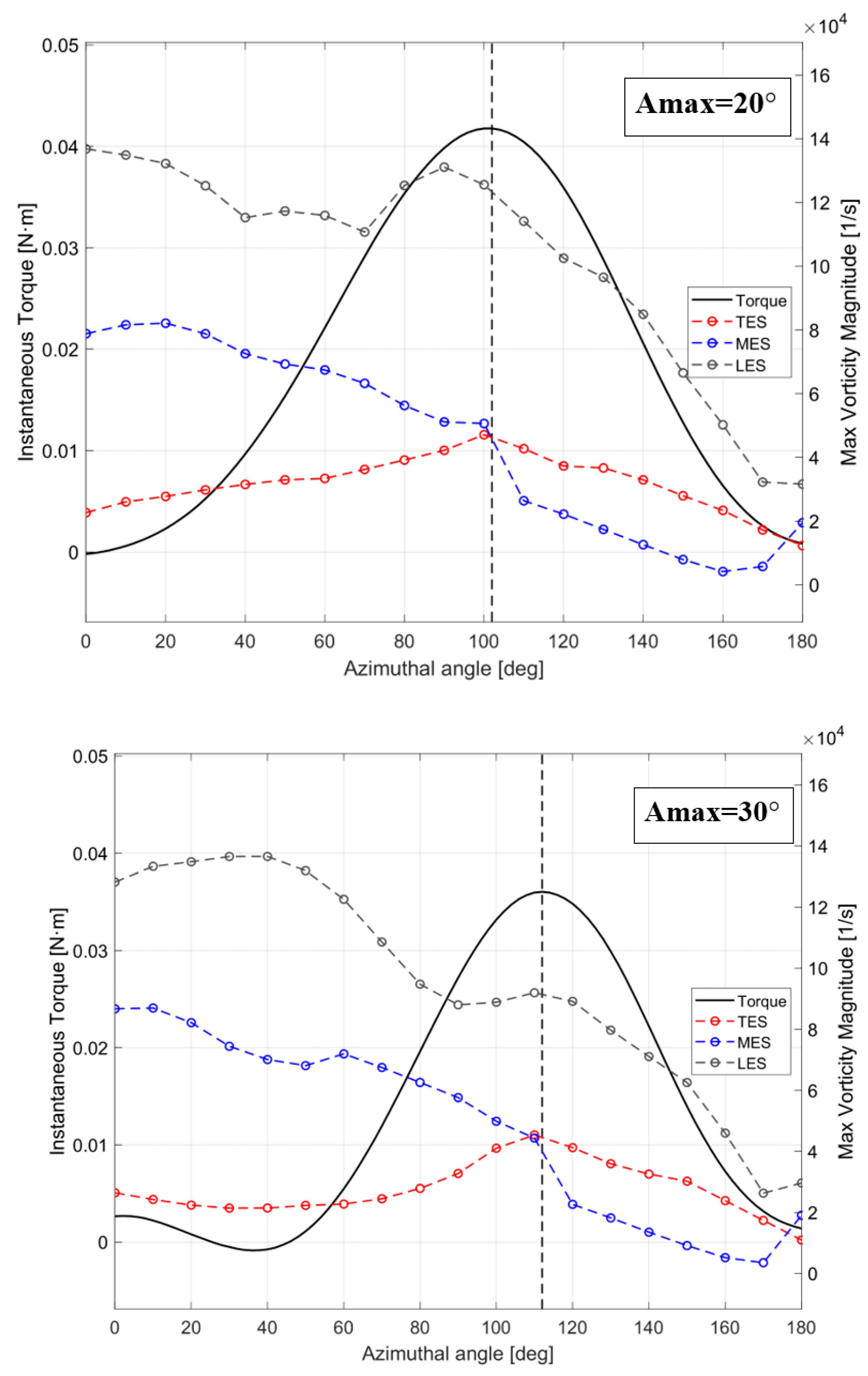
Figure 16 and Figure 17 present the instantaneous torque at the blade mid-span plane (Plane 1) for TSR = 0.5 and TSR = 1.4, respectively. Each figure also includes four instantaneous vorticity contour plots, shown in subplots ((a2)–(d2)), corresponding to pitch-angle amplitudes of 0° (a2), 10° (b2), 20° (c2), and 30° (d2). In addition, the evolution of the maximum vorticity at the LES, MES, and TES locations are reported, allowing a direct assessment of the relationship between vortex dynamics and torque generation.

As the blade rotates from θ = 0° to 360°, the vorticity distribution over the LES, MES, and TES evolves continuously and is closely associated with torque generation. Within this evolution, several characteristic points can be identified. For instance, when no variable pitch angle is applied, one can observe the following: (a) Point A (44°) corresponds to a local minimum of accumulated vorticity in the MES and marks the initial development of the vortex structure within this blade section; (b) Point B (46°) corresponds to the maximum vorticity at the LES which closely aligns with the highest instantaneous torque. The quantitative evolution of LES and MES vorticity indicates a transport and subsequent accumulation of vorticity from the LES toward the MES. Furthermore, Point C (56°) identifies the maximum vorticity at the MES and is associated with the onset Imminent Vortex Separation Condition (IVSC). Finally, Point D (64°) corresponds to vortex detachment, after which the vorticity magnitude decreases, and torque production is significantly reduced. These characteristic points provide quantitative evidence of the transport, accumulation, and release of vorticity during the dynamic stall process and their direct relationship with torque production.

Figure 16(a1)–(d1) further shows that, at TSR = 0.5, the decrease in instantaneous torque at Plane 1 (highlighted by the black dotted vertical line) is preceded by a reduction in LES vorticity (highlighted by the red dotted line). This torque decrease coincides with the onset of vorticity transport toward the MES, as evidenced by the subsequent increase in MES vorticity. Furthermore, the LES vorticity drop occurs at progressively larger azimuthal angles as the pitch-angle amplitude increases. Although the onset of vortex separation is identified at Point C through the IVSC criterion, the reduction in torque begins at smaller azimuthal angles, indicating that aerodynamic performance deterioration starts before complete vortex detachment. Across all pitch-angle amplitudes at TSR = 0.5, the characteristic vorticity evolution and the sequence of characteristic points remain qualitatively similar. This suggests that the underlying LES-to-MES vorticity transport mechanism is intrinsic to low-TSR operating conditions and persists regardless of the pitch-angle amplitude considered.

Figure 16(a2)–(d2) complements this analysis by presenting the corresponding vorticity contours at TSR = 0.5. Each subplot includes four snapshots (A–D), illustrating the spatial evolution of vorticity across the LES, MES, and TES regions. It is worth noting that, after condition C, where the maximum vorticity values at MES begin to decrease, the vortex appears to become detached, as qualitatively observed in the vorticity field at condition D. This qualitative observation is consistent with the quantitative identification of vortex separation provided by the IVSC criterion.

For TSR = 1.4, Figure 17 presents only the quantitative torque and vorticity results, since dynamic stall and vorticity transport are less pronounced at this operating condition. In this respect, one can note that the characteristic points A, B, C, and D identified in previous work [21] can still be observed at zero pitch amplitude (0°) for TSR = 1.4, as shown in Figure 17. However, as the pitch-angle amplitude increases to 10°, 20°, and 30°, these characteristic points become progressively less distinguishable. This behavior indicates a weakening of the vorticity transport, accumulation, and detachment mechanisms associated with dynamic stall, causing the quantitative vorticity signatures linked to the Imminent Vortex Separation Condition (IVSC) to become less pronounced.

Nevertheless, one can note in Figure 17 a consistent decrease in LES vorticity with this being consistent for all pitch-angle amplitudes at TSR = 1.4. This trend qualitatively follows the corresponding reduction in instantaneous torque, suggesting that a coupling between LES vorticity and torque generation persists even when dynamic stall effects are significantly attenuated. These results indicate that, although the IVSC-based framework is particularly valuable under low-TSR conditions where vortex transport mechanisms dominate the aerodynamic response, the relationship between leading-edge vorticity and torque production remains relevant across a broader range of operating conditions. Furthermore, the proposed methodology not only identifies the IVSC when vortex-driven mechanisms govern the aerodynamic response but also reveals when these mechanisms cease to be primary contributors to torque generation. In this respect, the progressive disappearance of the A–B–C–D characteristic flow condition at high TSR provides quantitative evidence of the transition from a vortex-dominated regime to an operating condition in which performance is increasingly controlled by changes in effective angle of attack and associated drag-related effects [22,23].

3.4. Vorticity and Torque Relationship

In our previous work [21], the relationship between vorticity and torque was examined at three blade sections: the Leading-Edge Section (LES), Mid-Edge Section (MES), and Trailing-Edge Section (TES). Among these, the LES exhibited the strongest and most consistent correlation with the instantaneous torque, indicating that this region dominates the early stages of dynamic stall and provides the most reliable indicator of aerodynamic performance.

It is important to consider, however, that the instantaneous torque results from the combined contributions of all blade sections (LES, MES, and TES). Consequently, although the LES captures the overall torque trend remarkably well, it does not perfectly coincide with the azimuthal location of the instantaneous torque peaks, as the latter reflects the integrated aerodynamic response of the entire blade.

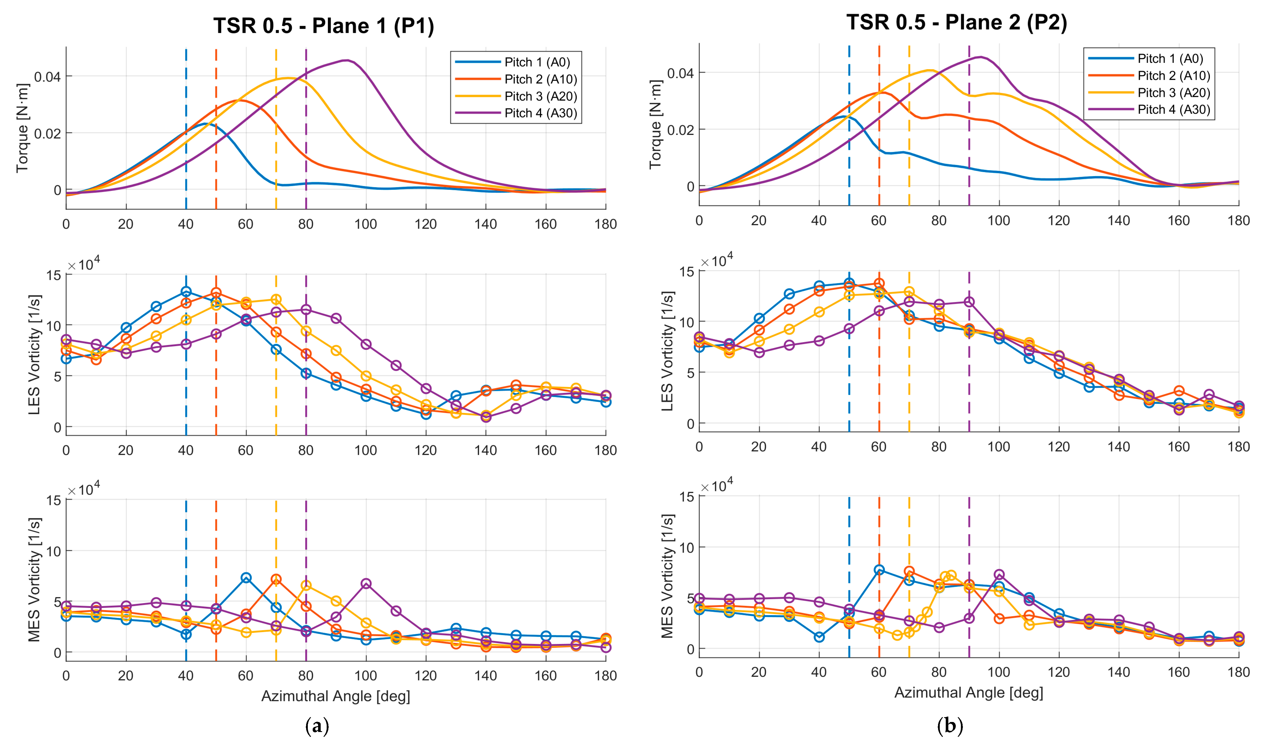
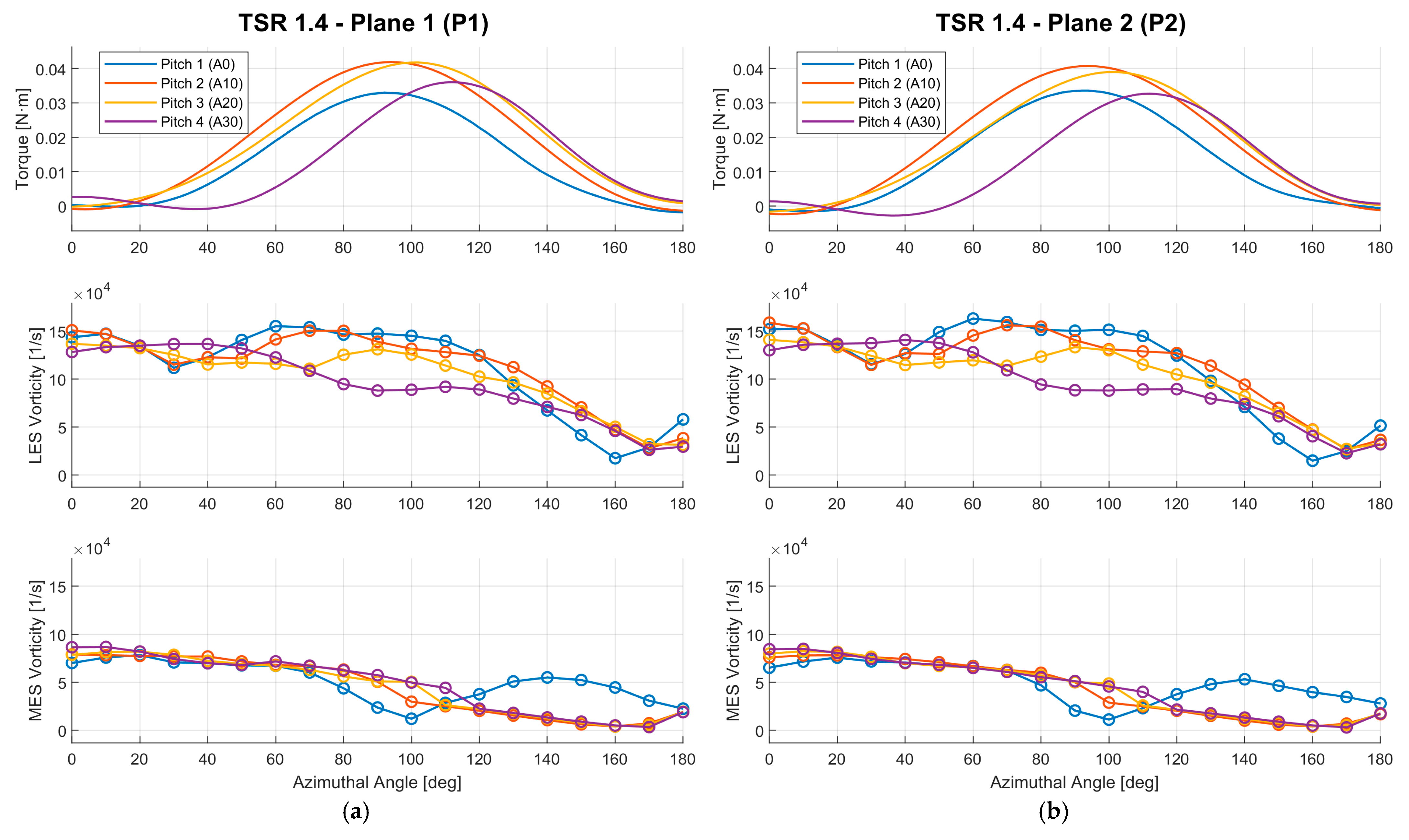
Building upon these findings, Figure 18 presents the quantitative vorticity distributions at the LES and MES sections for Plane 1 (a) and Plane 2 (b) at different pitch amplitudes of 0°, 10°, 20°, and 30°, as well as the instantaneous torque, providing direct evidence that the LES is the primary source of vorticity generation during the dynamic stall process.

The LES vorticity distributions shown in Figure 18a,b demonstrate that increasing the pitch-angle amplitude produces a systematic displacement of the LES and MES vorticity peak toward larger azimuthal angles. In this respect, as the pitch-angle amplitude increases from 0° to 30°, the maximum LES vorticity is shifted toward larger azimuthal angles, indicating that vortex formation and dynamic stall occur progressively later during blade rotation. As illustrated in Figure 18a,b, this divergence occurs at progressively larger azimuthal angles as the pitch amplitude increases, appearing at 60°, 70°, 90°, and 110° for pitch amplitudes of 0°, 10°, 20°, and 30°, respectively.

The comparison between the LES vorticity curves and the instantaneous torque evolution at TSR = 0.5 (Figure 18) further reveals that the maximum torque is closely associated with the maximum vorticity accumulation at the leading edge. Once the LES reaches its peak vorticity (Point B), the subsequent decrease in LES vorticity should not be interpreted as simple vortex dissipation. Instead, it marks the onset of a transport mechanism in which the vorticity generated at the leading edge is progressively convected and diffused toward the Mid-Edge Section (MES). For Plane 1, this process is evidenced by the dotted vertical lines, which show that as the LES vorticity begins to decrease, the MES vorticity increases almost simultaneously, indicating the downstream redistribution of vorticity along the blade surface.

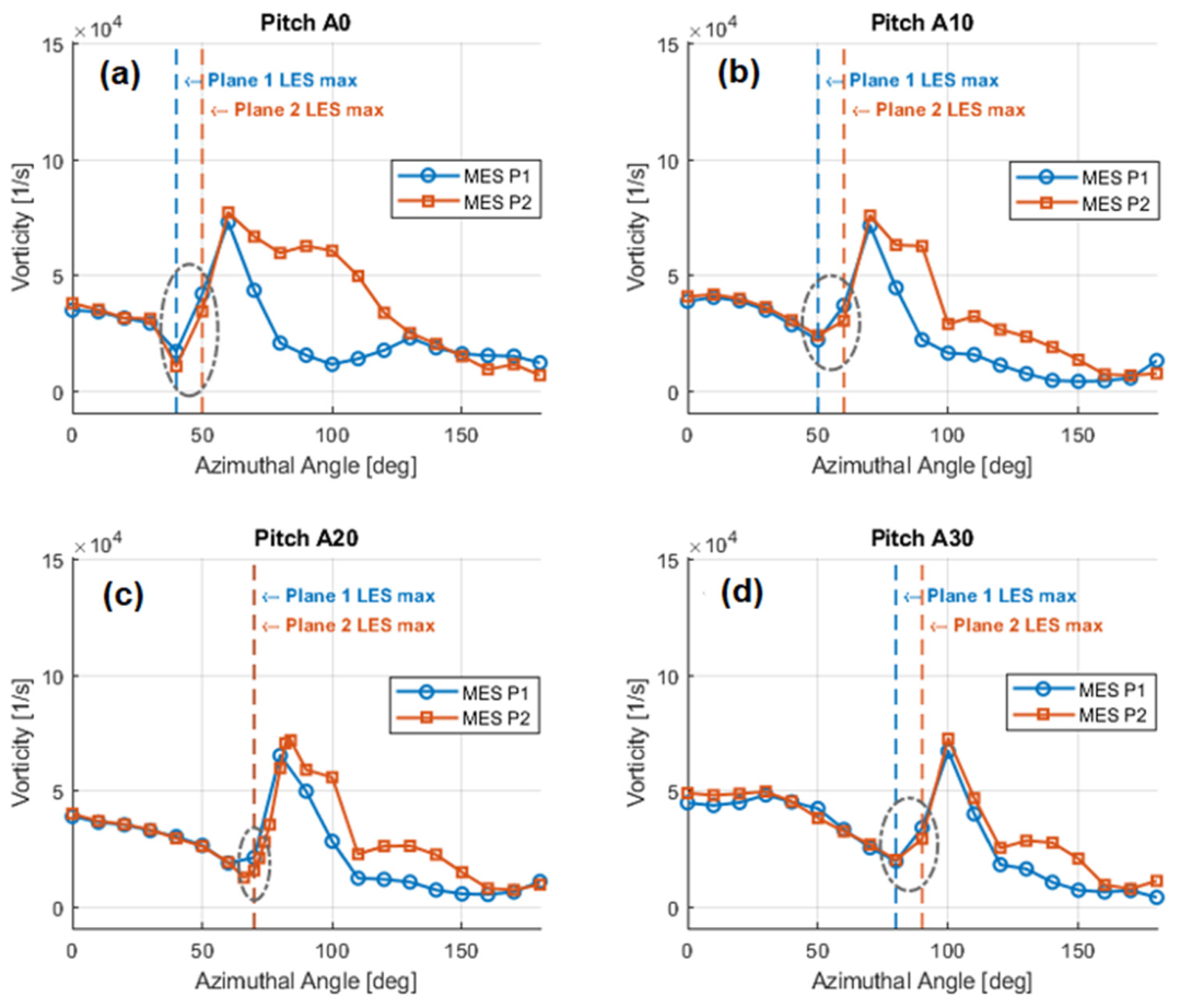
A different temporal evolution is observed for Plane 2. Unlike Plane 1, where the increase in MES vorticity closely follows the onset of LES vorticity decay, the MES vorticity begins to increase before the LES reaches its maximum value and starts to decrease. This early increase is highlighted by the dash-dotted oval in Figure 19a–d, a trend consistently observed across all evaluated pitch angle conditions. Since vorticity is conserved, this premature increase in MES vorticity cannot be explained by local vorticity generation within Plane 2 and must therefore result from the transport of vorticity from an upstream axial plane, such as Plane 1. This observation further demonstrates the capability of the proposed quantitative vorticity-analysis framework to identify and quantify not only the chordwise transport of vorticity along the blade surface (LES–MES), but also its axial transport between different blade planes, highlighting a key advantage of the present three-dimensional approach. Furthermore, this behavior is consistent with the higher instantaneous torque observed in Plane 2 compared with Plane 1, suggesting that the axially transported vorticity delays the onset of dynamic stall over the blade surface, thereby enhancing the aerodynamic loading.

Consequently, the reduction in LES vorticity should not be interpreted as simple vortex dissipation but rather as quantitative evidence of a transport mechanism that redistributes vorticity both along the blade surface and between axial planes.

In contrast to the dynamic stall-dominated behavior observed at TSR = 0.5, the vorticity evolution at TSR = 1.4 (Figure 20) exhibits significantly flatter profiles that remain elevated over a larger azimuthal range, reflecting the fundamentally different flow dynamics at this operating condition.

Unlike for TSR = 0.5, the highest pitch (30°) is no longer the best torque performer. Pitch 2 (10°) and Pitch 3 (20°) yield the highest peak torque, indicating that an intermediate pitch angle optimizes the effective angle of attack at higher speeds. For Pitch 4 (30°), vorticity drops prematurely around 70°, causing its torque curve to shift and peak later with a lower magnitude.

The proposed framework therefore provides objective evidence that the reduction in LES vorticity and the increase in MES vorticity are two complementary manifestations of the same physical phenomenon: the air transport process. Unlike conventional qualitative analyses based solely on instantaneous vorticity contours, the present methodology allows the complete evolution of the vortex to be quantified throughout the blade rotation. The LES vorticity curves demonstrate that the vortex development is not characterized simply by the appearance of high-vorticity regions, but by a well-defined temporal evolution involving generation, transport, accumulation, and eventual detachment of vorticity.

This LES-to-MES transport constitutes one of the key findings of the present work. Previous investigations generally relied on qualitative inspection of vorticity contours to infer vortex motion. In contrast, the present methodology demonstrates quantitatively that the decrease in LES vorticity, followed by the increase in MES vorticity, represents the physical mechanism through which fluid vorticity is accumulated prior to vortex separation. The maximum MES vorticity (Point C) corresponds to the Imminent Vortex Separation Condition (IVSC), which objectively identifies the onset of vortex detachment. Finally, Point D marks complete vortex detachment, after which both vorticity and torque decrease significantly.

This interpretation transforms the analysis from a qualitative description of vortex contours into a quantitative assessment of the physical mechanisms governing dynamic stall, providing a direct physical connection between vortex dynamics and torque production.

4. Conclusions

The present article addresses pitch variation in vertical-axis wind turbines (VAWTs) and the benefits on the modification of three-dimensional wake structure and tip vortex behavior, thereby influencing aerodynamics in the following ways:

(a)

It confirms via numerical simulation that in the variable-pitch VAWT, the power coefficient (C_p) augments by up to 237% and 58% at tip-speed ratios (TSRs) of 0.5 and 1.4, respectively.

(b)

It shows that increasing A_max at a TSR of 0.5 delays the onset of dynamic stall and reduces energy losses associated with uncontrolled vortex growth and detachment. This is evidenced by the shift in the Imminent Vortex Separation Condition (IVSC) to later azimuthal positions, as confirmed by quantitative vorticity analyses at the leading-edge (LES), mid-edge (MES), and trailing edge (TES) sections. These findings demonstrate that active pitch control improves flow attachment throughout the rotational cycle.

(c)

It characterizes a vortex-dynamics mechanism predominant at low TSRs (i.e., ≤1.2), where vorticity initially accumulates at the Leading-Edge Section (LES), generating maximum torque, before moving toward the Mid-Edge Section (MES). Its subsequent accumulation at the MES triggers the Imminent Vortex Separation Condition (IVSC), leading to vortex detachment. This mechanism is less predominant at TSRs > 1.2 operating in the drag region.

(d)

It demonstrates that the proposed vorticity analysis can successfully identify both the chordwise (LES-MES) and axial transport of vorticity at low TSRs, capturing the premature rise in MES vorticity in downstream planes, proving the methodology’s effectiveness in tracking three-dimensional flow interactions across the blade span.

References

1. Fossil Fuels Still Supply 84 Percent of World Energy—And Other Eye Openers from BP’s Annual Review. Available online: https://www.forbes.com/sites/rrapier/2020/06/20/bp-review-new-highs-in-global-energy-consumption-and-carbon-emissions-in-2019/?sh=692c741466a1 (accessed on 23 June 2026).
2. Fossil Fuels | EESI. Available online: https://www.eesi.org/topics/fossil-fuels/description (accessed on 23 June 2026).
3. Gerrie, C.; Islam, S.Z.; Gerrie, S.; Turner, N.; Asim, T. 3D CFD Modelling of Performance of a Vertical Axis Turbine. Energies 2023, 16, 1144. [Google Scholar] [CrossRef] [Scilit]
4. Ahmed, B.; Al Mubarak, M.; Khouj, M. Renewable Technologies: Solar Power and Wind Power Energy Utilization—Advantages and Disadvantages. In Technological Sustainability and Business Competitive Advantage; Al Mubarak, M., Hamdan, A., Eds.; Internet of Things; Springer International Publishing: Cham, Switzerland, 2023; pp. 507–519. [Google Scholar]
5. Vinoth Kanna, I.; Paturu, P. A Study of Hydrogen as an Alternative Fuel. Int. J. Ambient Energy 2020, 41, 1433–1436. [Google Scholar] [CrossRef] [Scilit]
6. Benghanem, M.; Mellit, A.; Almohamadi, H.; Haddad, S.; Chettibi, N.; Alanazi, A.M.; Dasalla, D.; Alzahrani, A. Hydrogen Production Methods Based on Solar and Wind Energy: A Review. Energies 2023, 16, 757. [Google Scholar] [CrossRef] [Scilit]
7. Mohtasham, J. Review Article-Renewable Energies. Energy Procedia 2015, 74, 1289–1297. [Google Scholar] [CrossRef] [Scilit]
8. Schubel, P.J.; Crossley, R.J. Wind Turbine Blade Design Review. Wind Eng. 2012, 36, 365–388. [Google Scholar] [CrossRef] [Scilit]
9. Li, S.; Dai, Y. Design and Simulation Analysis of a Small-Scale Compressed Air Energy Storage System Directly Driven by Vertical Axis Wind Turbine for Isolated Areas. J. Energy Eng. 2015, 141, 04014032. [Google Scholar] [CrossRef] [Scilit]
10. Ferreira, C.J.S.; Bijl, H.; Bussel, G.V.; Kuik, G.V. Simulating Dynamic Stall in a 2D VAWT: Modeling Strategy, Verification and Validation with Particle Image Velocimetry Data. J. Phys. Conf. Ser. 2007, 75, 012023. [Google Scholar] [CrossRef] [Scilit]
11. Le Fouest, S.; Mulleners, K. The Dynamic Stall Dilemma for Vertical-Axis Wind Turbines. Renew. Energy 2022, 198, 505–520. [Google Scholar] [CrossRef] [Scilit]
12. Souaissa, K.; Ghiss, M.; Chrigui, M.; Bentaher, H.; Maalej, A. A Comprehensive Analysis of Aerodynamic Flow around H-Darrieus Rotor with Camber-Bladed Profile. Wind Eng. 2019, 43, 459–475. [Google Scholar] [CrossRef] [Scilit]
13. Jiang, Y.; He, C.; Zhao, P.; Sun, T. Investigation of Blade Tip Shape for Improving VAWT Performance. J. Mar. Sci. Eng. 2020, 8, 225. [Google Scholar] [CrossRef] [Scilit]
14. Visbal, M.R.; Garmann, D.J. Dynamic Stall of a Finite-Aspect-Ratio Wing. AIAA J. 2019, 57, 962–977. [Google Scholar] [CrossRef] [Scilit]
15. Bianchini, A.; Balduzzi, F.; Bachant, P.; Ferrara, G.; Ferrari, L. Effectiveness of Two-Dimensional CFD Simulations for Darrieus VAWTs: A Combined Numerical and Experimental Assessment. Energy Convers. Manag. 2017, 136, 318–328. [Google Scholar] [CrossRef] [Scilit]
16. Balduzzi, F.; Drofelnik, J.; Bianchini, A.; Ferrara, G.; Ferrari, L.; Campobasso, M.S. Darrieus Wind Turbine Blade Unsteady Aerodynamics: A Three-Dimensional Navier-Stokes CFD Assessment. Energy 2017, 128, 550–563. [Google Scholar] [CrossRef] [Scilit]
17. Balduzzi, F.; Bianchini, A.; Maleci, R.; Ferrara, G.; Ferrari, L. Critical Issues in the CFD Simulation of Darrieus Wind Turbines. Renew. Energy 2016, 85, 419–435. [Google Scholar] [CrossRef] [Scilit]
18. Fertahi, S.e.-D.; Samaouali, A.; Kadiri, I. CFD Comparison of 2D and 3D Aerodynamics in H-Darrieus Prototype Wake. E-Prime-Adv. Electr. Eng. Electron. Energy 2023, 4, 100178. [Google Scholar] [CrossRef] [Scilit]
19. Nazari, S.; Zamani, M.; Moshizi, S.A. Comparison between Two-Dimensional and Three-Dimensional Computational Fluid Dynamics Techniques for Two Straight-Bladed Vertical-Axis Wind Turbines in Inline Arrangement. Wind Eng. 2018, 42, 647–664. [Google Scholar] [CrossRef] [Scilit]
20. Franchina, N.; Persico, G.; Savini, M. 2D-3D Computations of a Vertical Axis Wind Turbine Flow Field: Modeling Issues and Physical Interpretations. Renew. Energy 2019, 136, 1170–1189. [Google Scholar] [CrossRef] [Scilit]
21. Escudero Romero, A.; Blasetti, A.P.; Acosta-López, J.G.; Gómez-García, M.-Á.; De Lasa, H. Vorticity and Its Relationship to Vortex Separation, Dynamic Stall, and Performance, in an H-Darrieus Vertical-Axis Wind Turbine Using CFD Simulations. Processes 2024, 12, 1556. [Google Scholar] [CrossRef] [Scilit]
22. Sagharichi, A.; Maghrebi, M.J.; ArabGolarcheh, A. Variable Pitch Blades: An Approach for Improving Performance of Darrieus Wind Turbine. J. Renew. Sustain. Energy 2016, 8, 053305. [Google Scholar] [CrossRef] [Scilit]
23. Sagharichi, A.; Zamani, M.; Ghasemi, A. Effect of Solidity on the Performance of Variable-Pitch Vertical Axis Wind Turbine. Energy 2018, 161, 753–775. [Google Scholar] [CrossRef] [Scilit]
24. Abdalrahman, G.; Daoud, M.A.; Melek, W.W.; Lien, F.-S.; Yee, E. Design and Implementation of an Intelligent Blade Pitch Control System and Stability Analysis for a Small Darrieus Vertical-Axis Wind Turbine. Energies 2021, 15, 235. [Google Scholar] [CrossRef] [Scilit]
25. Rezaeiha, A.; Kalkman, I.; Blocken, B. Effect of Pitch Angle on Power Performance and Aerodynamics of a Vertical Axis Wind Turbine. Appl. Energy 2017, 197, 132–150. [Google Scholar] [CrossRef] [Scilit]
26. Zhao, Z.; Wang, R.; Shen, W.; Wang, T.; Xu, B.; Zheng, Y.; Qian, S. Variable Pitch Approach for Performance Improving of Straight-Bladed VAWT at Rated Tip Speed Ratio. Appl. Sci. 2018, 8, 957. [Google Scholar] [CrossRef] [Scilit]
27. Hammad, M.A.; Mahmoud, A.M.; Abdelrhman, A.M.; Sarip, S. Performance Enhancement of H-Type Darrieus VAWT Using a Hybrid Method of Blade Pitch Angle Regulation. Energies 2024, 17, 4044. [Google Scholar] [CrossRef] [Scilit]
28. Chen, L.; Yang, Y.; Gao, Y.; Gao, Z.; Guo, Y.; Sun, L. A Novel Real-Time Feedback Pitch Angle Control System for Vertical-Axis Wind Turbines. J. Wind Eng. Ind. Aerodyn. 2019, 195, 104023. [Google Scholar] [CrossRef] [Scilit]
29. Zhang, Q.; Bashir, M.; Miao, W.; Liu, Q.; Li, C.; Yue, M.; Wang, P. Aerodynamic Analysis of a Novel Pitch Control Strategy and Parameter Combination for Vertical Axis Wind Turbines. Renew. Energy 2023, 216, 119089. [Google Scholar] [CrossRef] [Scilit]
30. Melani, P.F.; Balduzzi, F.; Brandetti, L.; Ferreira, C.S.; Bianchini, A. An Experimental and Numerical Analysis of the Dynamic Variation of the Angle of Attack in a Vertical-Axis Wind Turbine. J. Phys. Conf. Ser. 2020, 1618, 052064. [Google Scholar] [CrossRef] [Scilit]
31. Asadbeigi, M.; Ghafoorian, F.; Mehrpooya, M.; Chegini, S.; Jarrahian, A. A 3D Study of the Darrieus Wind Turbine with Auxiliary Blades and Economic Analysis Based on an Optimal Design from a Parametric Investigation. Sustainability 2023, 15, 4684. [Google Scholar] [CrossRef] [Scilit]
32. Ardaneh, F.; Abdolahifar, A.; Karimian, S.M.H. Numerical Analysis of the Pitch Angle Effect on the Performance Improvement and Flow Characteristics of the 3-PB Darrieus Vertical Axis Wind Turbine. Energy 2022, 239, 122339. [Google Scholar] [CrossRef] [Scilit]
33. Sanaye, S.; Rezaeian, P.; Farvizi, A. A Novel Surrogated Approach for Optimizing a Vertical Axis Wind Turbine with Straight Blades. Wind Energy 2024, 27, 953–974. [Google Scholar] [CrossRef] [Scilit]
34. Elkhoury, M.; Kiwata, T.; Aoun, E. Experimental and Numerical Investigation of a Three-Dimensional Vertical-Axis Wind Turbine with Variable-Pitch. J. Wind Eng. Ind. Aerodyn. 2015, 139, 111–123. [Google Scholar] [CrossRef] [Scilit]
35. Yan, Y.; Avital, E.; Williams, J.; Cui, J. CFD Analysis for the Performance of Micro-Vortex Generator on Aerofoil and Vertical Axis Turbine. J. Renew. Sustain. Energy 2019, 11, 043302. [Google Scholar] [CrossRef] [Scilit]
36. Syawitri, T.P.; Yao, Y.; Yao, J.; Chandra, B. A Review on the Use of Passive Flow Control Devices as Performance Enhancement of Lift-type Vertical Axis Wind Turbines. WIREs Energy Environ. 2022, 11, e435. [Google Scholar] [CrossRef] [Scilit]
37. Ma, N.; Lei, H.; Han, Z.; Zhou, D.; Bao, Y.; Zhang, K.; Zhou, L.; Chen, C. Airfoil Optimization to Improve Power Performance of a High-Solidity Vertical Axis Wind Turbine at a Moderate Tip Speed Ratio. Energy 2018, 150, 236–252. [Google Scholar] [CrossRef] [Scilit]
38. Kheradvar, A.; Pedrizzetti, G. Vortex Formation in the Cardiovascular System; Springer: London, UK, 2012. [Google Scholar]
39. Wu, J.C. Elements of Vorticity Aerodynamics; Springer Tracts in Mechanical Engineering; Springer: Berlin/Heidelberg, Germany, 2018. [Google Scholar]
40. Wu, J.-Z.; Ma, H.-Y.; Zhou, M.-D. Vorticity and Vortex Dynamics; Springer: Berlin/Heidelberg, Germany, 2006. [Google Scholar]
41. Acosta-López, J.G.; Blasetti, A.P.; Lopez-Zamora, S.; De Lasa, H. CFD Modeling of an H-Type Darrieus VAWT under High Winds: The Vorticity Index and the Imminent Vortex Separation Condition. Processes 2023, 11, 644. [Google Scholar] [CrossRef] [Scilit]
42. Navier–Stokes Equations Equations-Wikipedia. Available online: https://en.wikipedia.org/wiki/Navier%E2%80%93Stokes_equations (accessed on 23 June 2026).
43. Menter, F.R. Two-Equation Eddy-Viscosity Turbulence Models for Engineering Applications. AIAA J. 1994, 32, 1598–1605. [Google Scholar] [CrossRef] [Scilit] [PubMed]
44. Wong, K.H.; Chong, W.T.; Poh, S.C.; Shiah, Y.-C.; Sukiman, N.L.; Wang, C.-T. 3D CFD Simulation and Parametric Study of a Flat Plate Deflector for Vertical Axis Wind Turbine. Renew. Energy 2018, 129, 32–55. [Google Scholar] [CrossRef] [Scilit]
45. Dyachuk, E. Aerodynamics of Vertical Axis Wind Turbines: Development of Simulation Tools and Experiments; Digital Comprehensive Summaries of Uppsala Dissertations from the Faculty of Science and Technology; Acta Universitatis Upsaliensis: Uppsala, Sweden, 2015. [Google Scholar]
46. Dong, L.; Choi, K.-S.; Mao, X. Interplay of the Leading-Edge Vortex and the Tip Vortex of a Low-Aspect-Ratio Thin Wing. Exp. Fluids 2020, 61, 200. [Google Scholar] [CrossRef] [Scilit]
Figure 1. Computational fixed and rotating domains adopted for CFD calculations.
Processes 14 02778 g001
Figure 2. Projection of the mesh considered in the simulations on both the airfoil and on the near-airfoil region.
Processes 14 02778 g002
Figure 3. Representation of the 3D computational mesh of the hexahedral domain used in the present study.
Processes 14 02778 g003
Figure 4. Mesh dependency (Cp values for Blade 1 at TSR = 1.4, and a 2° march time-step).
Processes 14 02778 g004
Figure 5. Timestep dependency (Cp values for Blade 1, at TSR = 1.4, and using fine size mesh).
Processes 14 02778 g005
Figure 6. Cp comparison of 3D CFD with experimental data [34,37].
Processes 14 02778 g006
Figure 7. Angles of attack ( α ) during one rotation at different TSRs ( α angle is calculated from Equation (7) taken from [41]).
Processes 14 02778 g007
Figure 8. Applied forces on a VAWT blade, with description of α acceptance angle for (a) fixed blade, (b) variable-pitch-angle blade. Note: a = U·sin(θ), b = U·cos(θ), and α = arctan ( sin ( θ ) / ( cos ( θ ) + TSR ) .
Processes 14 02778 g008
Figure 9. Geometric angles of attack α during one rotation at TSR = 1.4 when employing (i) fixed-pitch angle of attack; (ii) variable-pitch angle of attack with A m a x = 10 ° ; (iii) variable-pitch angle of attack with A m a x = 20 ° ; (iv) variable-pitch angle of attack with A m a x = 30 ° .
Processes 14 02778 g009
Figure 10. Horizontal section planes, at the various vertical airfoil levels considered in this study.
Processes 14 02778 g010
Figure 11. Cross-section of the airfoil (dashed red line) showing the LES, the MES, the TES sections at Plane 1.
Processes 14 02778 g011
Figure 12. Cp versus maximum amplitude at TSR of 0.5 & 1.4.
Processes 14 02778 g012
Figure 13. Instantaneous torque for planes 1 to 3 and Amax from 0° to 30° at TSR = 0.5. Note: Reference to horizontal Planes 1, 2 and 3 of airfoil position given in Figure 10.
Processes 14 02778 g013
Figure 14. Instantaneous torque for planes 1 to 3 and Amax changing from 0° to 30° at TSR = 1.4.
Processes 14 02778 g014
Figure 15. Instantaneous torque at Plane 1 for TSR = 0.5 (a) and TSR = 1.4 (b), for fixed pitch and variable pitch amplitudes of 10°, 20°, and 30°.
Processes 14 02778 g015
Figure 16. (a1d1) Instantaneous torque and maximum vorticity at the leading-edge (LES), mid-edge (MES), and trailing-edge (TES) sections (left column). (a2d2) Instantaneous vorticity contours at Plane 1 (mid-span) (right column) for TSR = 0.5 showing the leading-edge (LES), mid-edge (MES), and trailing-edge (TES) regions at four characteristic moments (A–D). Each row corresponds to a different maximum pitch amplitude: (a1) 0°, (b1) 10°, (c1) 20°, and (d1) 30°. Vertical dashed lines indicate azimuthal angles where maximum instantaneous torque (black) and maximum LES vorticity (red) occur.
Processes 14 02778 g016aProcesses 14 02778 g016bProcesses 14 02778 g016cProcesses 14 02778 g016dProcesses 14 02778 g016e
Figure 17. Maximum vorticity values at LES, MES and TES (dotted lines), and instantaneous torque at Plane 1 (full line) for TSR = 0.5 for fixed pitch and variable pitch amplitudes of 10°, 20°, and 30°. Vertical dashed lines indicate the azimuthal angles where the maximum instantaneous torque (black dashed line) occurs.
Processes 14 02778 g017aProcesses 14 02778 g017b
Figure 18. Instantaneous torque and vorticity values at LES and MES at (a) Plane 1 and (b) Plane 2 for TSR = 0.5 for fixed pitch and maximum pitch amplitudes of 10°, 20°, and 30°. Vertical dashed lines (Ai) indicate the onset of LES vorticity decay for each operating condition.
Processes 14 02778 g018
Figure 19. MES vorticity comparison between Plane 1 and Plane 2 at TSR = 0.5 for (a) fixed pitch (A0) and maximum pitch amplitudes of (b) 10° (A10), (c) 20° (A20), and (d) 30° (A30). Vertical dashed lines indicate the specific azimuthal angle of maximum LES vorticity (onset of LES decay) for each respective plane. The dash-dotted gray oval highlights the early increase in MES vorticity observed in Plane 2 prior to the onset of LES decay, illustrating the phase shift and axial transport effects between planes.
Processes 14 02778 g019
Figure 20. Instantaneous torque and vorticity values at LES and MES at (a) Plane 1 and (b) Plane 2 for TSR = 1.4 for fixed pitch and maximum pitch amplitudes of 10°, 20°, and 30°.
Processes 14 02778 g020