Numerical Investigation of Gas Dispersion, Drag-Coefficient Distribution, and Mixing Performance in a Rushton-Turbine Stirred Tank Using a Euler–Euler Model

Abstract

Gas dispersion and liquid circulation are critical factors governing the performance of gas–liquid stirred tanks, yet the coupled effects of operating conditions and impeller geometry on hydrodynamic behavior remain insufficiently understood. In this study, a Euler–Euler two-fluid model coupled with the standard k–ε turbulence model is employed to investigate gas dispersion, drag-coefficient distribution, power consumption, and mixing dead zones in a Rushton turbine stirred tank. The numerical model is validated against published experimental data before examining the influences of impeller rotational speed, gas injection velocity, blade height, and blade length. The results reveal that high drag coefficients are concentrated along the impeller discharge path, vortex-core regions and near-wall annular structures, indicating zones of reduced gas–liquid slip and strong interphase momentum exchange. Increasing the stirring speed from 400 to 800 rpm reduces the fluid and liquid dead-zone fractions from 93.31% to 54.27% and from 24.64% to 12.08%, respectively, but increases the power from 8.78 to 77.00 W. By contrast, increasing the gas-injection velocity from 5 to 13 m/s decreases the power draw but expands the fluid dead-zone fraction from 50.94% to 94.54%, indicating a marked deterioration in effective liquid circulation associated with gas accumulation near the impeller. Blade height mainly adjusts local shear and gas-holdup uniformity, whereas blade length is the dominant geometric parameter for dead-zone suppression, although its benefit becomes marginal at the largest length because of the severe power penalty. These findings clarify the coupled effects of gas dispersion, liquid circulation, drag-coefficient distribution, and power demand, and provide guidance for the design and operation of gas–liquid stirred tanks.

1. Introduction

Gas–liquid stirred tanks have been prevalently employed in the chemical, biological, pharmaceutical, and metallurgical industries owing to their enhanced heat/mass transfer coefficients, substantial interfacial contact area, and operational flexibility [1,2,3,4,5]. Within these systems, mixing performance, gas holdup, and power consumption are principally governed by operational variables and impeller geometric configurations [6,7,8,9,10,11,12]. Notably, during multiphase flow evolution, flow pattern metamorphosis critically modulates interfacial momentum transfer mechanisms, thus dictating the macroscopic hydrodynamic performance of stirred tank reactors. The macroscopic hydrodynamic characteristics emerge as manifestations of multiscale interactions between dispersed gas phases and continuous liquid flows [13,14]. In the stirring systems, the useful hydrodynamic performance is not determined by gas holdup alone. It also depends on whether the impeller-generated circulation can maintain gas dispersion without excessive power consumption or the formation of poorly mixed low-velocity zones. Therefore, a design-relevant analysis must connect the local two-phase flow structure with global indicators such as power draw and dead-zone volume.

The hydrodynamics of gas–liquid two-phase systems in stirred reactors are recognized as complex phenomena dominated by interfacial interactions and bubble coalescence/breakup mechanisms [15,16,17,18,19]. Non-invasive measurement techniques such as particle image velocimetry (PIV) and laser Doppler velocimetry (LDA) have been extensively adopted to explore flow field characteristics in multiphase reactors owing to minimal flow disturbance and high-resolution spatiotemporal data acquisition capabilities [20,21,22,23]. Kolano et al. [24] employed PIV techniques to investigate viscoelastic flow pattern transitions (axial/compartmentalized/radial) in stirred tanks, demonstrating that these transitions are governed by the elasticity number El, with tip speed-normalized velocity fields following log-normal distributions in both elastic and turbulent regimes. Aubin et al. [25] revealed through PIV that up-pumping pitched blade turbines enhance global gas holdup by 36% over down-pumping configurations in aerated tanks, with unaltered turbulent kinetic energy near the impeller (favoring bubble breakup) and superior liquid circulation dynamics. Schäfer et al. [26] utilized refractive index-matched laser Doppler velocimetry (LDV) to characterize flow fields in a Rushton turbine-stirred reactor, identifying peak turbulent kinetic energy (0.08U_tip²) in trailing vortex-dominated radial jet regions and energy dissipation length scales of D/8.71, providing high-resolution datasets for CFD validation and impeller optimization. Benayad et al. [27] investigated velocity-concentration interactions in a continuous stirred tank reactor based on LDV and conductivity probes, revealing that axial velocity-concentration correlations remained below 5%, turbulent diffusivity reached 4000 times molecular levels, and velocity/concentration fluctuations exhibited near-Gaussian distributions beyond the impeller zone, supporting local isotropic turbulence and enhanced mixing models. However, PIV and LDV techniques struggle to resolve microscopic flow parameters (e.g., turbulent energy and dissipation rates) and are constrained by optical measurement under high-temperature and high-pressure operating conditions, profoundly impeding flow field characterization. To obtain insights into the optimal design of gas–liquid mixing tanks based on the hydrodynamics of gas–liquid two-phase tanks, it is necessary to study the gas dispersion behavior and mixing characteristics in detail during the gas–liquid two-phase mixing process.

The development of computational fluid dynamics (CFD) has positioned it as an indispensable tool for characterizing multiphase flow patterns, enabled by advances in high-performance computing [28,29,30,31]. The CFD technology provides real-time visualization and predictive capabilities for transient turbulent flows in gas–liquid stirred reactors, particularly effective for resolving complex phenomena involving stochastic phase interactions and energy dissipation [32,33,34,35,36,37]. In this approach, the gas–liquid two-phase flow is predicted by the Euler–Euler method, in which both the continuous phase (water) and the dispersed phase (air) are treated as a continuous interpenetrating medium [38,39]. Tamburini et al. [40] compared the applicability of k-ω SST, k-ε, and SSG turbulence models in non-baffled and baffled stirred vessels via CFD simulations, revealing that SSG outperformed at high Reynolds numbers in non-baffled systems while k-ω SST was more accurate at low Reynolds numbers, with no significant differences among the three models in baffled configurations. Xu et al. [41] employed the CFD-Taguchi method to optimize power consumption and oxygen transfer efficiency for C5 sugar acid production in gas–liquid stirred bioreactors, demonstrating that while the wide-blade hydrofoil (WHd) excelled in energy efficiency at low speeds and the concave blade disk turbine (CBDT) achieved superior oxygen transfer at high speeds, the Rushton turbine (RT) offered the best overall balance, with agitation speed identified as the predominant influencing factor. Chen et al. [42] conducted numerical simulations of the gas–liquid two-phase flow field in a horizontal stirred tank, disclosing the influence of rotational speed, gas flow rate, and impeller structural parameters (inclination angle, off-bottom height) on gas phase distribution uniformity, liquid phase mixing efficiency, and power characteristics, thereby providing a theoretical basis for the optimal design of industrial stirred tanks. Li et al. [43] analyzed the hydrodynamic characteristics of forward-reverse rotating impellers in a non-baffled stirred tank through computational fluid dynamics (CFD) simulations, elucidating periodic flow field variations and the “zoned flow” phenomenon (where different rotation directions induce partitioned fluid motion), with the average power number significantly higher than that in traditional constant-speed stirred tanks with or without baffles, providing theoretical foundations for optimizing stirred equipment design. Bao et al. [44] carried out numerical simulations and experimental investigations on gas–liquid two-phase flow in multi-impeller stirred tanks to systematically analyze the effects of impeller diameter and superficial gas velocity on local gas holdup and bubble size distribution, concluding that smaller impeller diameter (D/T = 0.30) under identical power input conditions generate higher local gas holdup and more uniform bubble distribution while bubble size is primarily governed by superficial gas velocity, thereby providing quantitative guidance for the optimal design of industrial stirred tanks. Previous CFD studies have investigated the effects of turbulence models, impeller types, gas flow rate, impeller diameter, rotational speed, and geometric configurations on gas holdup, power consumption, and mixing performance. These works have improved the understanding of gas–liquid flow in stirred tanks and have demonstrated the usefulness of CFD for reactor design and optimization. Despite these advances, most existing numerical studies still focus mainly on separate descriptions of gas holdup, velocity distribution, or power consumption. Less attention has been paid to the coupled relationship among interphase drag, gas dispersion, liquid circulation, and mixing dead zones. This limitation is important because gas dispersion and mixing performance are not controlled by gas holdup alone. A high gas holdup may improve gas–liquid contact, but excessive gas accumulation near the impeller can weaken liquid pumping, reduce effective circulation, and enlarge stagnant regions. Similarly, a reduction in power consumption under aerated conditions does not necessarily indicate improved mixing, because it may result from gas cavity formation and reduced impeller loading. Therefore, a coupled analysis of interphase drag, gas distribution, power consumption, and dead-zone evolution is needed to clarify the hydrodynamic mechanisms that control energy-efficient gas–liquid mixing.

In the present study, a Euler–Euler two-fluid model coupled with the standard k–ε turbulence model is used to investigate gas–liquid flow in a Rushton turbine stirred tank. The numerical model is first validated against published experimental data for liquid velocity and gas holdup. The validated model is then applied to analyze the spatial distributions of gas holdup, phase velocity, and interphase drag coefficient. Particular attention is paid to the effects of impeller rotational speed, gas injection velocity, blade height, and blade length on power consumption and mixing dead zones. The objective is not merely to perform a parametric CFD study, but to clarify how operating and geometric parameters regulate gas dispersion and mixing performance through interphase momentum transfer.

2. Mathematical Model

2.1. Governing Equations

The Eulerian-Eulerian (E-E) multiphase approach is implemented in this study. In this approach, both continuous and dispersed phases are considered as continuous interpenetrating media based on their volume fractions. This is followed by solving the continuity and momentum equations using the E-E approach for each phase. Equations (1) and (2) show the continuity and conversion of momentum for phase q, respectively:

$${\displaystyle \frac{\partial \left({\alpha }_q{\rho }_q\right)}{\partial t}}+\nabla \cdot \left({\alpha }_q{\rho }_q{\mathit{u}}_q\right)=0$$

(1)

$${\displaystyle \frac{\partial \left({\alpha }_q{\rho }_q{\mathit{u}}_q\right)}{\partial t}}+\nabla \cdot \left({\alpha }_q{\rho }_q{\mathit{u}}_q{\mathit{u}}_q\right)=-{\alpha }_q\nabla P+\nabla \cdot ({\mu }_{eff,q}{\alpha }_q(\nabla {\mathit{u}}_q+(\nabla {{\mathit{u}}_q)}^T))+{\alpha }_q{\rho }_q\mathit{g}+{\mathit{F}}_{\mathit{i}\mathit{n}\mathit{t}\mathit{e}\mathit{r}}$$

(2)

where α_q is the phasic volume fraction, in which the sum of the volume fractions of the gas and liquid phases is constant at 1 (α_l + α_g = 1). Ρ_q and u_q indicate the density and velocity vector for the q-th phase in the computational domain, respectively. P, μ_eff,q, and g stand for the fluid pressure, effective viscosity, and gravity acceleration, respectively. The symbol F_inter represents the sum of the interaction forces between the phases, comprising drag (F_D), lift (F_L), turbulent dispersion (F_TD), wall lubrication (F_WL), and virtual mass (F_VM).

$${\mathit{F}}_{\mathit{i}\mathit{n}\mathit{t}\mathit{e}\mathit{r}}={\mathit{F}}_{\mathit{D}}+{\mathit{F}}_{\mathit{L}}+{\mathit{F}}_{\mathit{T}\mathit{D}}+{\mathit{F}}_{\mathit{W}\mathit{L}}+{\mathit{F}}_{\mathit{V}\mathit{M}}$$

(3)

2.2. Interfacial Momentum Transfer

According to Scargiali et al. [45], the main non-drag forces exert relatively small overall effects in mechanically stirred gas–liquid systems, and turbulent dispersion has negligible impact on predicted gas distribution. Therefore, only the drag force is accounted for interphase momentum transfer in this study, while lift, turbulent-dispersion, wall-lubrication, and virtual-mass forces are omitted. The interphase momentum-transfer term is thus simplified to the drag-force contribution. The drag force between gas and liquid phases is expressed as follows:

$${\mathit{F}}_{\mathit{i}\mathit{n}\mathit{t}\mathit{e}\mathit{r}}={\mathit{F}}_{\mathit{D}}={\displaystyle \frac{3}{4}}{\alpha }_g{\rho }_l{\displaystyle \frac{C_D}{d_b}}\left|{\mathit{u}}_{\mathit{g}}-{\mathit{u}}_{\mathit{l}}\right|({\mathit{u}}_{\mathit{g}}-{\mathit{u}}_{\mathit{l}})$$

(4)

where d_b is the diameter of the bubble. C_D is the drag coefficient. In the present work, the Schiller–Naumann drag model is adopted, which defines the drag coefficient separately according to two different ranges of the bubble Reynolds number (Re_b).

$$C_D=\left\{\begin{array}{l}{\displaystyle \frac{24}{{\mathrm{Re}}_b}}(1+0.15{\mathrm{Re}}_b^{0.687}),{\mathrm{Re}}_b\le 1000\\ 0.44,{\mathrm{Re}}_b>1000\end{array}\right.$$

(5)

$${\mathrm{Re}}_b={\displaystyle \frac{{\rho }_l{d}_b\left|{\mathit{u}}_{\mathit{g}}-{\mathit{u}}_{\mathit{l}}\right|}{{\mu }_l}}$$

(6)

The Reynolds time-averaged standard k-ε model is used for the turbulence equations to describe the gas–liquid two-phase turbulent flow in the stirred tank. It is a semi-empirical model based on the transport equations for the turbulence kinetic energy (k) and the turbulence dissipation rate (ε). Izzah et al. [46] systematically compared five turbulence models within the Reynolds-Averaged Navier–Stokes (RANS) framework, including the Spalart–Allmaras, standard k-ε, RNG k-ε, standard k-ω, and Reynolds Stress Model (RSM). The research demonstrated that although the standard k–ε model can qualitatively capture the flow field trends, it tends to underpredict both tangential and axial velocities in quantitative predictions. However, the standard k–ε model has been widely adopted in practical engineering fluid computations due to its reasonable accuracy and computational economy [47]. No explicit bubble-induced turbulence contribution, such as a Sato-type model, was included in the present simulations. Therefore, the possible influence of bubble-generated turbulence on local turbulence intensity and phase distribution, particularly in regions of relatively high gas holdup, represents a limitation of the present model and will be further investigated in future work. The equations of the turbulent kinetic energy k and turbulent dissipation rate ε are given in the following form:

$${\displaystyle \frac{\partial }{\partial x_i}}\left(\rho k{\mathit{u}}_i\right)={\displaystyle \frac{\partial }{\partial x_j}}((\mu +{\displaystyle \frac{{\mu }_t}{{\sigma }_k}}){\displaystyle \frac{\partial k}{\partial x_j}})-{\displaystyle \frac{\partial }{\partial t}}(\rho k)+G_k-\rho \epsilon$$

(7)

$${\displaystyle \frac{\partial }{\partial x_i}}\left(\rho k{\mathit{u}}_i\right)={\displaystyle \frac{\partial }{\partial x_j}}((\mu +{\displaystyle \frac{{\mu }_t}{{\sigma }_{\epsilon }}}){\displaystyle \frac{\partial \epsilon }{\partial x_j}})-{\displaystyle \frac{\partial }{\partial t}}(\rho \epsilon )+{\displaystyle \frac{C_{1\epsilon }\epsilon }{k}}{G}_k-C_{2\epsilon }\rho {\displaystyle \frac{{\epsilon }^2}{k}}$$

(8)

$${\mu }_t=\rho C_{\mu }{\displaystyle \frac{k^2}{\epsilon }}$$

(9)

where μ_t is turbulent viscosity and G_k denotes the turbulent kinetic energy generated by the mean velocity gradient. C_1ε, C_2ε, σ_k, σ_ε, and C_µ are model constants determined by basic turbulence experiments, with default values of 1.44, 1.92, 1.0, 1.3, and 0.09, respectively.

3. Computational Settings

3.1. Simulation Configuration

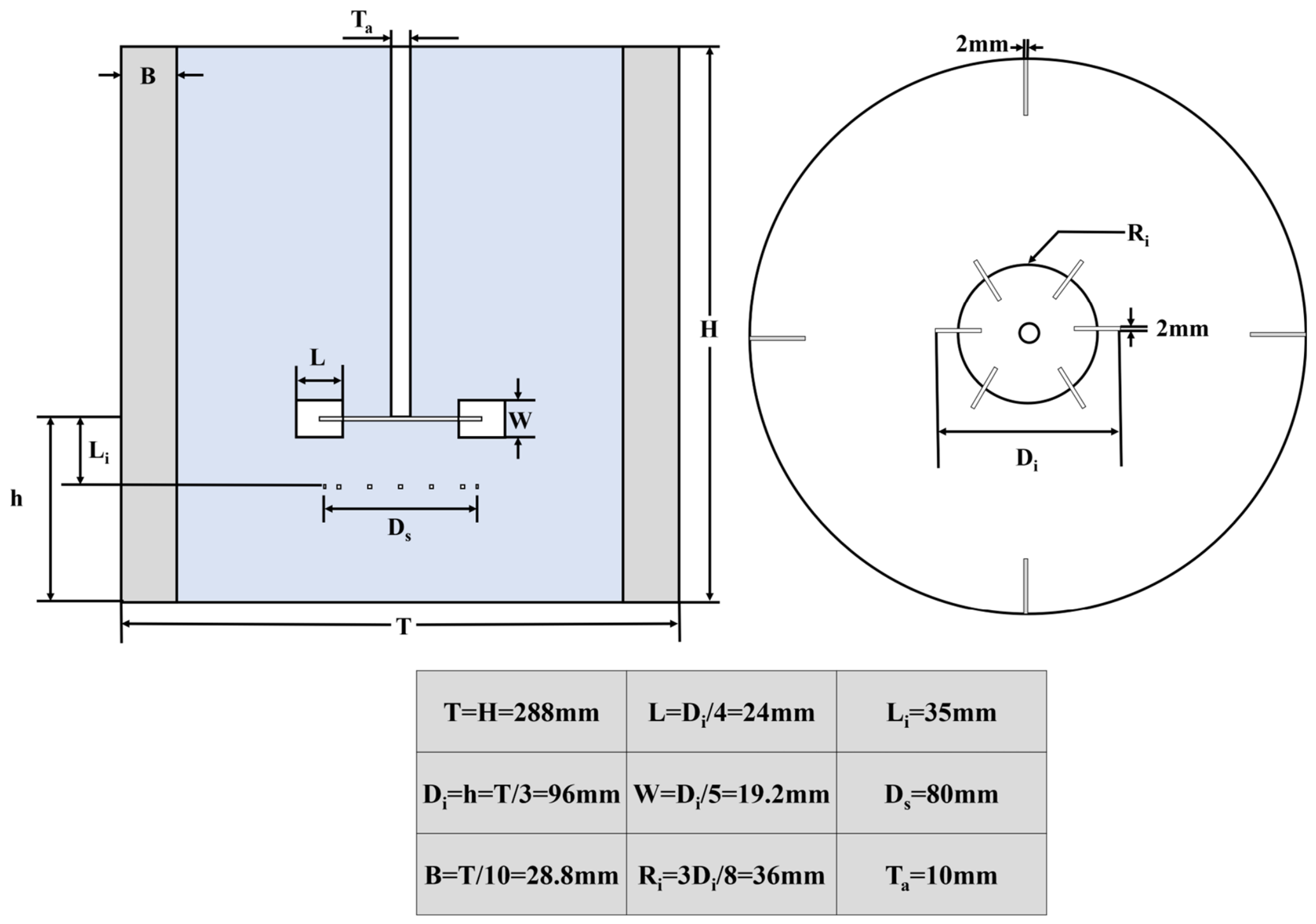
The complete geometric details of the gas–liquid stirred tank are illustrated in Figure 1. The geometric configuration is selected based on the benchmark baffled Rushton-turbine stirred tank reported by Guan et al. [48], whose experimental data are used for subsequent model validation. The principal geometric ratios are maintained consistently with this benchmark configuration to enable direct comparison between the present CFD predictions and the published experimental measurements. In addition, the baffled Rushton-turbine configuration represents a conventional radial-flow system for investigating gas–liquid dispersion in mechanically stirred tanks. The gas–liquid stirred tank consists of a flat-bottomed cylindrical vessel with a diameter T = 0.288 m and a height H equal to the value of T. Four baffles with a width of T/10 and a thickness of 2 mm are installed perpendicular to the vessel wall. The agitation system utilizes a six-bladed Rushton turbine impeller, which has an impeller diameter of D_i = T/3, a blade length L = D_i/4, a blade height W = D_i/5, and a thickness of 2 mm. The impeller clearance from the bottom (h) is equal to T/3. The diameter of the agitator shaft (T_a) is 10 mm. Gas was introduced through an annular distributor located 35 mm below the impeller (L_i). The distributor diameter was 80 mm and contained 12 uniformly distributed orifices, each with a diameter of 2 mm. A constant representative bubble diameter of d_b = 1 mm is specified in the Euler–Euler simulations and is kept unchanged for all investigated impeller rotational speeds, gas-injection velocities, blade lengths, and blade heights. The applicability of this numerical setting is assessed through the model validation presented in Section 3.3 using experimental liquid-phase velocity and gas-holdup data.

The gas inlet was specified as a velocity inlet with a gas volume fraction of 1. The tank top was treated using a degassing boundary condition, allowing the gas phase to leave the domain while retaining the liquid phase. No-slip wall conditions were imposed on the tank wall, baffles, shaft, and impeller surfaces. The liquid phase was tap water with a density of 998.2 kg/m³ and a dynamic viscosity of 1.003 × 10⁻³ Pa·s. The gas phase was air with a density of 1.225 kg/m³ and a dynamic viscosity of 1.7894 × 10⁻⁵ Pa·s. The impeller rotation is modeled via the multiple reference frame (MRF) approach, whereas the rest of the tank domain is treated in a stationary reference frame. The standard k-ε turbulence model is employed with gravity enabled. The gas–liquid two-phase flow is solved under steady-state conditions using the coupled algorithm. The MRF approach is selected for its computational efficiency in obtaining steady approximations of global hydrodynamic features and for consistent comparisons across diverse operating and geometric conditions in this work. Nevertheless, since the relative position between rotating and stationary zones is fixed within the MRF formulation, blade-passing effects and other time-dependent flow structures are not explicitly resolved. As a result, transient phenomena including the development of trailing vortices, gas cavities, and local gas-holdup fluctuations cannot be directly captured by these steady-state simulations. The computational domain is divided into a stationary region and an MRF rotating region surrounding the Rushton turbine. The rotating region has a diameter of 152 mm and a height of 56 mm, with the impeller located at its center. Local mesh refinement was applied around the impeller and in regions with strong flow gradients. The selected mesh contained approximately 5.60 × 10⁵ cells, with a minimum orthogonal quality of 0.759. The near-wall mesh resolution was further evaluated using the dimensionless wall distance ${\mathrm{y}}^{+}$. Under the baseline operating condition, the area-weighted average ${\mathrm{y}}^{+}$ values on the tank wall, impeller, and baffles were 19.66, 32.23, and 16.50, respectively. The relatively higher ${\mathrm{y}}^{+}$ value on the impeller surface is associated with the stronger wall shear generated in the blade-swept region. These results provide an additional quantitative assessment of the near-wall mesh resolution used in the present simulations. The steady-state calculations are performed using the pressure-based coupled algorithm with the global time-step pseudo-time method. The solver-control parameters and relaxation factors are maintained at the default Fluent settings throughout the simulations, with no additional stepwise solver constraints imposed. The default Fluent residual convergence criteria are adopted to assess numerical convergence. The baseline case is N = 600 rpm, Ug = 9 m/s, L = 24 mm, and W = 19.2 mm, and each series varies only one of these four parameters while the others remain fixed. The corresponding parameter as shown in

Table 1. Parametric simulation conditions.

Group	Stirring Speed Si (rpm)	Gas Injection Velocity Ug (m/s)	Blade Length Li (mm)	Blade Height Hi (mm)
1	400	5	19	17.2
2	500	7	24 *	19.2 *
3	600 *	9 *	29	21.2
4	700	11	34	23.2
5	700	13	39	25.2

Note: * denotes the baseline value used in the reference condition.

.

3.2. Performance Indicators

The impeller power consumption is calculated from the torque acting on the impeller:

$$P = 2\pi {\displaystyle \frac{N}{60}}M$$

(10)

where P is the power consumption (W), N is the impeller rotational speed (rpm), and M is the torque (N·m). The liquid-phase and mixture dead-zone fraction was evaluated using a velocity-based criterion.

To characterize the overall motion of the gas–liquid mixture, the mixture velocity is calculated using the local phase-volume-fraction-weighted velocities of the gas and liquid phases:

$${\mathit{U}}_{mix}={\alpha }_g{\mathit{U}}_g+{\alpha }_l{\mathit{U}}_l$$

(11)

where U_mix, U_g, and U_l denote the mixture, gas, and liquid phase velocities, respectively, while α_g and α_l are the corresponding local phase volume fractions, satisfying (α_g + α_l = 1).

The liquid-phase and mixture dead-zone fractions are evaluated using a velocity-based criterion. Following the velocity-based dead-zone definition reported by Leonzio et al. and Trad et al. [49,50], regions where the local velocity magnitude is lower than 5% of the corresponding maximum velocity in the computational domain were identified as dead zones. Specifically, the liquid-phase dead zone is determined from the liquid-phase velocity field, whereas the mixture-phase dead zone is determined from the mixture velocity field. For the mixture phase, the magnitude of U_mix calculated from Equation (11) is used for dead-zone identification. For each simulation case, the corresponding maximum velocity is extracted independently from the converged flow field rather than using a universal fixed characteristic velocity for all operating conditions. This relative criterion normalizes the local velocity with respect to the characteristic flow intensity of each case and provides a consistent dimensionless basis for comparing low-velocity regions under different rotational speeds, gas injection velocities, and impeller geometries. The dead-zone volume fraction, defined as the ratio of the dead-zone volume to the total tank volume, was therefore used as a comparative indicator of mixing performance. The 5% threshold is literature-based and has been used as a consistent comparative criterion for dead-zone evaluation [49,50]. Nevertheless, the absolute dead-zone fraction may depend on the selected threshold, and sensitivity analyses using alternative thresholds, such as 3% and 10%, will be considered in future work.

3.3. Model Validation

3.3.1. Validation I: Grid-Independence

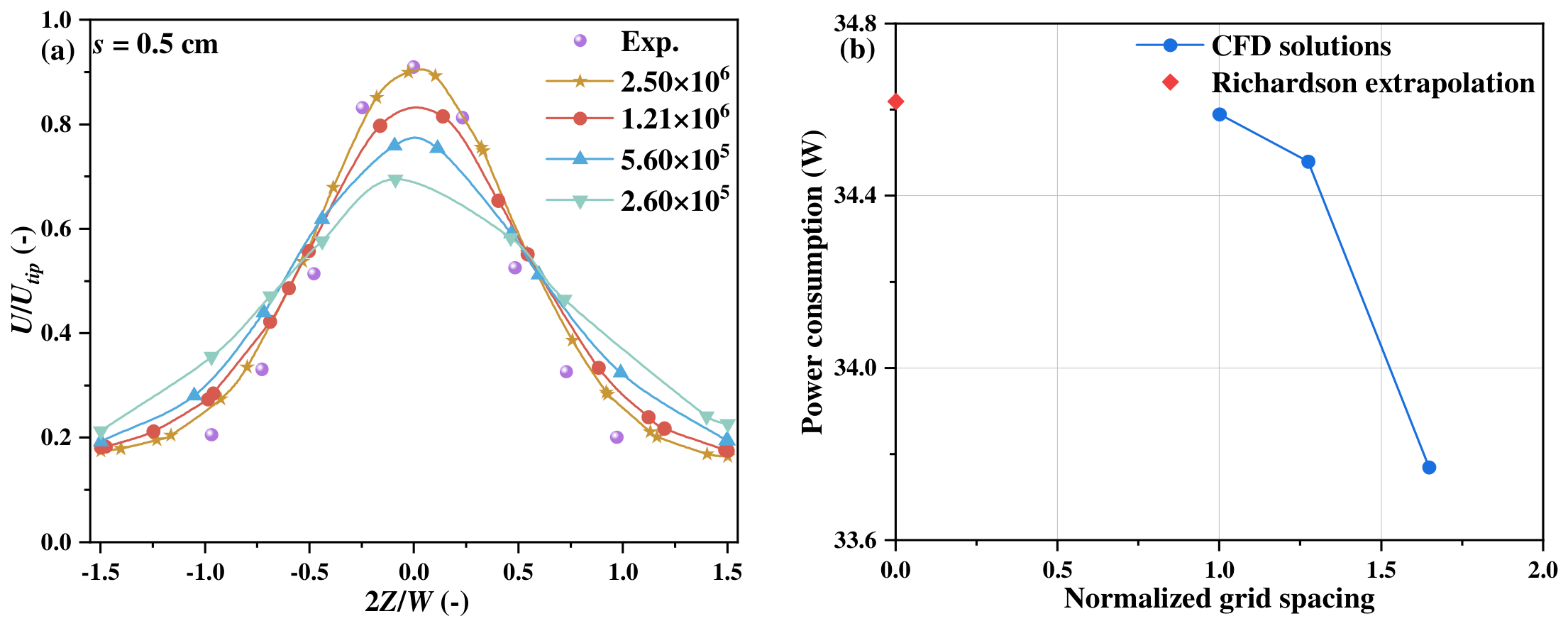
A grid-independence assessment is conducted using four meshes containing 2.60 × 10⁵, 5.60 × 10⁵, 1.21 × 10⁶, and 2.50 × 10⁶ computational cells. The coordinate origin Z = 0 m corresponds to the centre of the impeller disk, where W and s denote the height of the blade and the radial distance from the impeller blade tip, respectively. The accuracy of the simulation results is evaluated by comparison with experimental data, where the experimental data for both single-phase flow and gas–liquid flow are derived from the research conducted by Guan et al. [48]. As shown in Figure 2, all four meshes reproduce the characteristic bell-shaped velocity profile in the impeller discharge zone. The velocity maximum occurs near the impeller mid-plane (2Z/W = 0) and decreases toward both sides. With mesh refinement, the strong velocity gradient in the high-shear discharge region is resolved more clearly, while the overall profile shape and peak position remain consistent.

To provide a quantitative basis for mesh selection, the impeller power consumption is further evaluated according to Equation (10). The power consumptions obtained with the 2.60 × 10⁵, 5.60 × 10⁵, 1.21 × 10⁶, and 2.50 × 10⁶ cells are 33.07, 33.77, 34.48, and 34.59 W, respectively. The relative difference between the 5.60 × 10⁵ and 1.21 × 10⁶ cells is only 2.06%.

The Grid Convergence Index (GCI) method combined with Richardson extrapolation is further employed following Celik et al. [51] to quantify the spatial discretization convergence. For the present three-dimensional computational domain, the representative grid spacing of the $\mathrm{i}$th mesh is defined as:

$$h_i = {({\displaystyle \frac{V}{N_i}})}^{1/3}$$

(12)

where $\mathrm{V}$ is the computational-domain volume and ${\mathrm{N}}_{\mathrm{i}}$ is the total number of computational cells. Since the same computational domain is used for all meshes, the normalized grid spacing is expressed as:

$${\displaystyle \frac{h_i}{h_1}} = {({\displaystyle \frac{N_1}{N_i}})}^{1/3}$$

(13)

Grid 1, Grid 2, and Grid 3 correspond to the 2.50 × 10⁶, 1.21 × 10⁶, and 5.60 × 10⁵ cell meshes, respectively. Consequently, their normalized grid spacings are 1.000, 1.274, and 1.647, respectively, and the corresponding effective refinement ratios are ${\mathrm{r}}_{21}=1.274$ and ${\mathrm{r}}_{32}=1.293$. Based on the three numerical solutions, the apparent order of convergence is calculated to be $p=7.073$.

The Richardson-extrapolated impeller power is subsequently determined from the two finest-grid solutions as

$$P_{ext}=P_1+{\displaystyle \frac{P_1-P_2}{r_{21}^p-1}}$$

(14)

Substituting ${\mathrm{P}}_1=34.59384$ W, ${\mathrm{P}}_2=34.48101$ W, ${\mathrm{r}}_{21}=1.27365$, and $p=7.0729$ gives:

$$P_{ext}=34.61873 \mathrm{W}$$

(15)

This value represents the estimated asymptotic solution as the grid spacing approaches zero and is represented by the red diamond at zero normalized grid spacing in Figure 2b.

The relative differences between two successive grid solutions are defined as:

$${\epsilon }_{12}= {\displaystyle \frac{P_2-P_1}{P_1}}$$

(16)

$${\epsilon }_{23}={\displaystyle \frac{P_3-P_2}{P_2}}$$

(17)

Using the safety factor of ${\mathrm{F}}_{\mathrm{s}}=1.25$, the corresponding Grid Convergence Indices are calculated as:

$$GC{I}_{12}= {\displaystyle \frac{F_s\left|{\epsilon }_{12}\right|}{r_{21}^p-1}}\times 100\%$$

(18)

$$GC{I}_{23}={\displaystyle \frac{F_s\left|{\epsilon }_{23}\right|}{r_{32}^p-1}}\times 100\%$$

(19)

The calculated values are GCI₁₂ = 0.09% and GCI₁₂ = 0.5%. The asymptotic consistency ratio is evaluated as:

$$R_{asym}={\displaystyle \frac{GC{I}_{23}}{r_{21}^{p}GC{I}_{12}}}$$

(20)

The asymptotic consistency ratio is 1.003, which is close to unity and supports the consistency of the three-grid GCI analysis. The corresponding coarse-grid GCI for the selected 5.60 × 10⁵ cell is GCI_coarse = 3.07%, providing a quantitative estimate of its discretization uncertainty for the predicted impeller power.

As shown in Figure 2b, the calculated impeller power progressively approaches the Richardson-extrapolated value with mesh refinement. The 5.60 × 10⁵ cell is the coarsest mesh within the three-grid sequence exhibiting consistent asymptotic convergence. Its predicted impeller power differs from that obtained with the 1.21 × 10⁶ cell by only 2.06% and from the Richardson-extrapolated value by approximately 2.45%, while its estimated discretization uncertainty is approximately 3.07%. Considering these quantitative results together with the substantially lower computational cost required for the extensive parametric simulations, the mesh containing 5.60 × 10⁵ cells is selected for all subsequent calculations.

3.3.2. Validation II: Single Phase

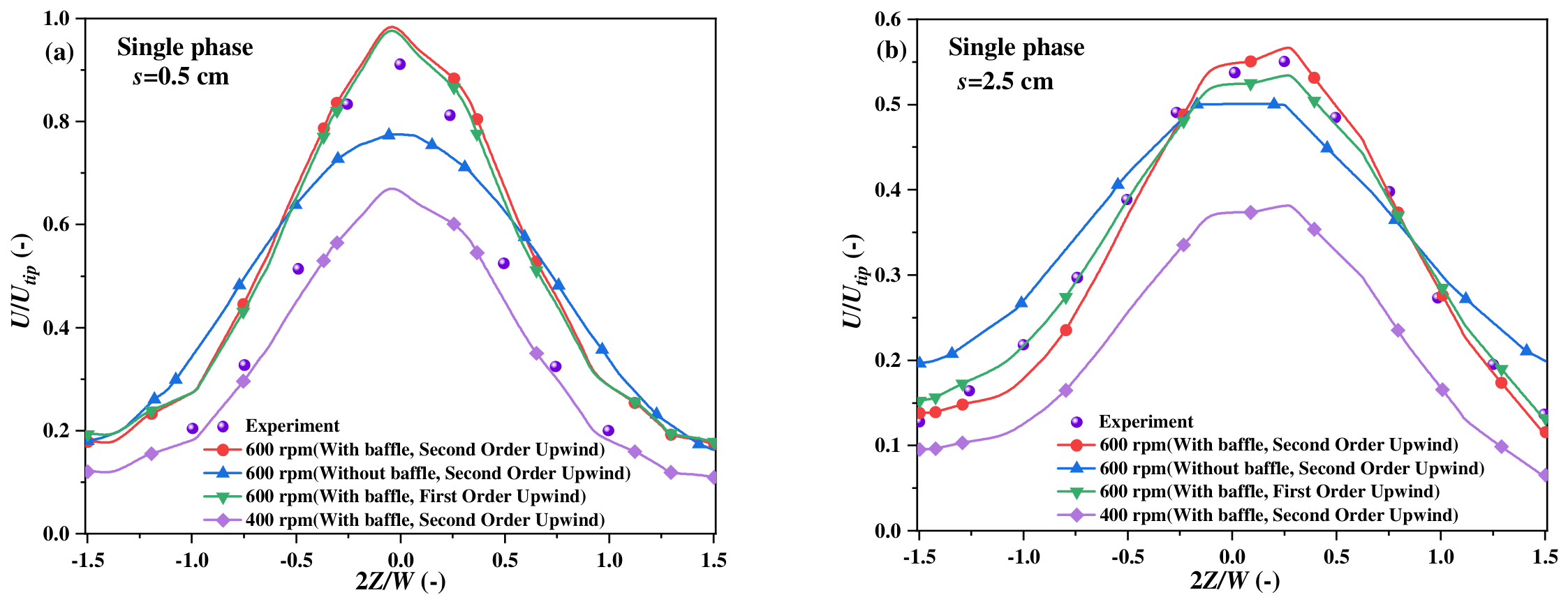
For complex multiphase Computational fluid dynamics (CFD) calculations, it is essential to initially necessary to obtain complete predictions for a single-phase system and validate these results with detailed experimental data. The predicted axial distribution of normalized liquid velocity for different radial locations is illustrated in Figure 3. The coordinate origin Z = 0 m corresponds to the centre of the impeller disk, where W and s denote the height of the blade and the radial distance from the impeller blade tip, respectively. The second-order upwind scheme with baffles at 400 rpm underestimates the liquid velocity at all radial positions due to the limited turbulent energy provided by the low rotational speed (400 rpm). At s = 0.5 cm, the first- and second-order upwind schemes with baffles at 600 rpm yield nearly identical predictions, both overestimating the liquid velocity at all axial positions. The second-order upwind scheme without baffles at 600 rpm underestimates the liquid velocity near the impeller disc plane section while showing an opposite trend with increasing axial position. The deviations of the first- and second-order upwind schemes with baffles at 600 rpm intensify with increasing radial distance. At s = 2.5 cm, the first-order upwind scheme with baffles at 600 rpm provides optimal predictions, demonstrating perfect agreement with experimental measurements. Moreover, the axial position of velocity peaks shifts slightly upward with increasing radial position, a trend that the first-order upwind scheme with baffles at 600 rpm appears to capture. Overall, the first-order upwind scheme with baffles at 600 rpm improves prediction accuracy while maintaining lower computational costs. Therefore, this study adopts the first-order upwind scheme with baffles at 600 rpm for simulations. However, this closer agreement should not be interpreted as evidence of the intrinsic superiority of the first-order scheme, because the associated numerical diffusion may affect the resolved velocity gradients. The sensitivity to higher-order discretization will be further investigated in future work.

3.3.3. Validation III: Gas–Liquid Phase

Drag is the dominant force impacting the hydrodynamic characteristics of gas–liquid two-phase flow in stirred tanks. The present validation primarily assesses the capability of the numerical model to reproduce the liquid-phase velocity and gas-holdup distributions. The spatial drag-coefficient field and the dead-zone fraction are model-derived quantities and have not been independently validated against direct experimental measurements. In the present Euler–Euler framework, the local drag coefficient is calculated using the Schiller–Naumann correlation as a function of the bubble Reynolds number and the gas–liquid relative velocity. Therefore, its spatial distribution is dependent on the resolved two-phase hydrodynamics and is constrained by the validated velocity and gas-holdup fields.

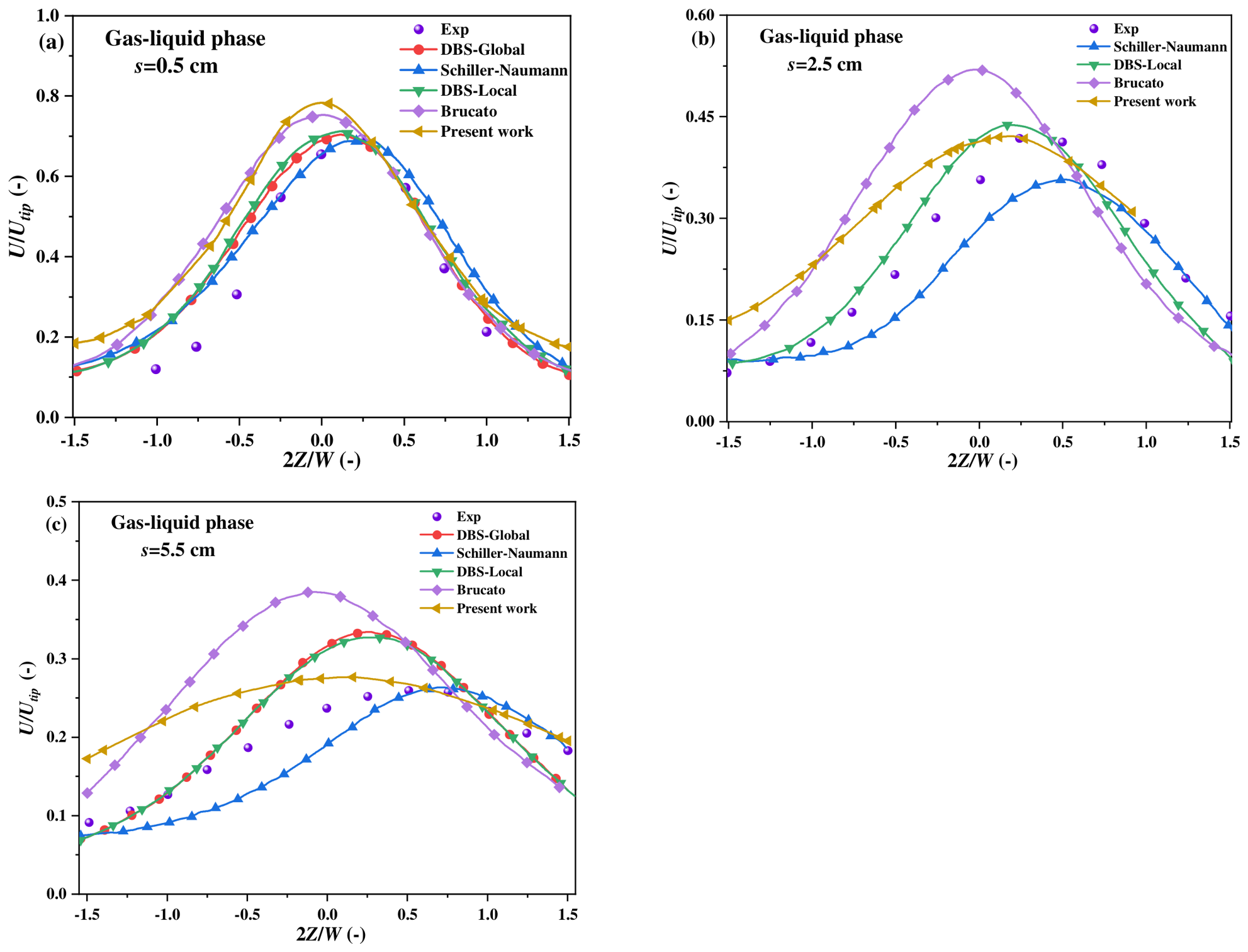
Figure 4 compares the normalized liquid-velocity axial distribution predicted by the present work with the experimental measurements and the numerical results reported by Guan et al. [48] using four different drag models, namely Schiller–Naumann, Brucato, DBS-Global, and DBS-Local, at three radial positions (s = 0.5, 2.5, and 5.5 cm). It should be noted that the curve labelled “Present work” represents the prediction obtained using the numerical model adopted in the present study, whereas the other four different drag models are taken from Guan et al. [48]. The different drag models successfully capture the characteristic bell-shaped velocity distribution in the impeller discharge region, although noticeable differences are observed in the predicted peak velocity and profile shape. The present work slightly overpredicts the liquid velocity below the impeller disk at all three measurement locations, while showing good agreement with the experimental data above the impeller disk. In general, the present CFD model provides reliable predictions of the liquid-phase hydrodynamics in the impeller discharge region, demonstrating the good predictive capability of the adopted numerical methodology.

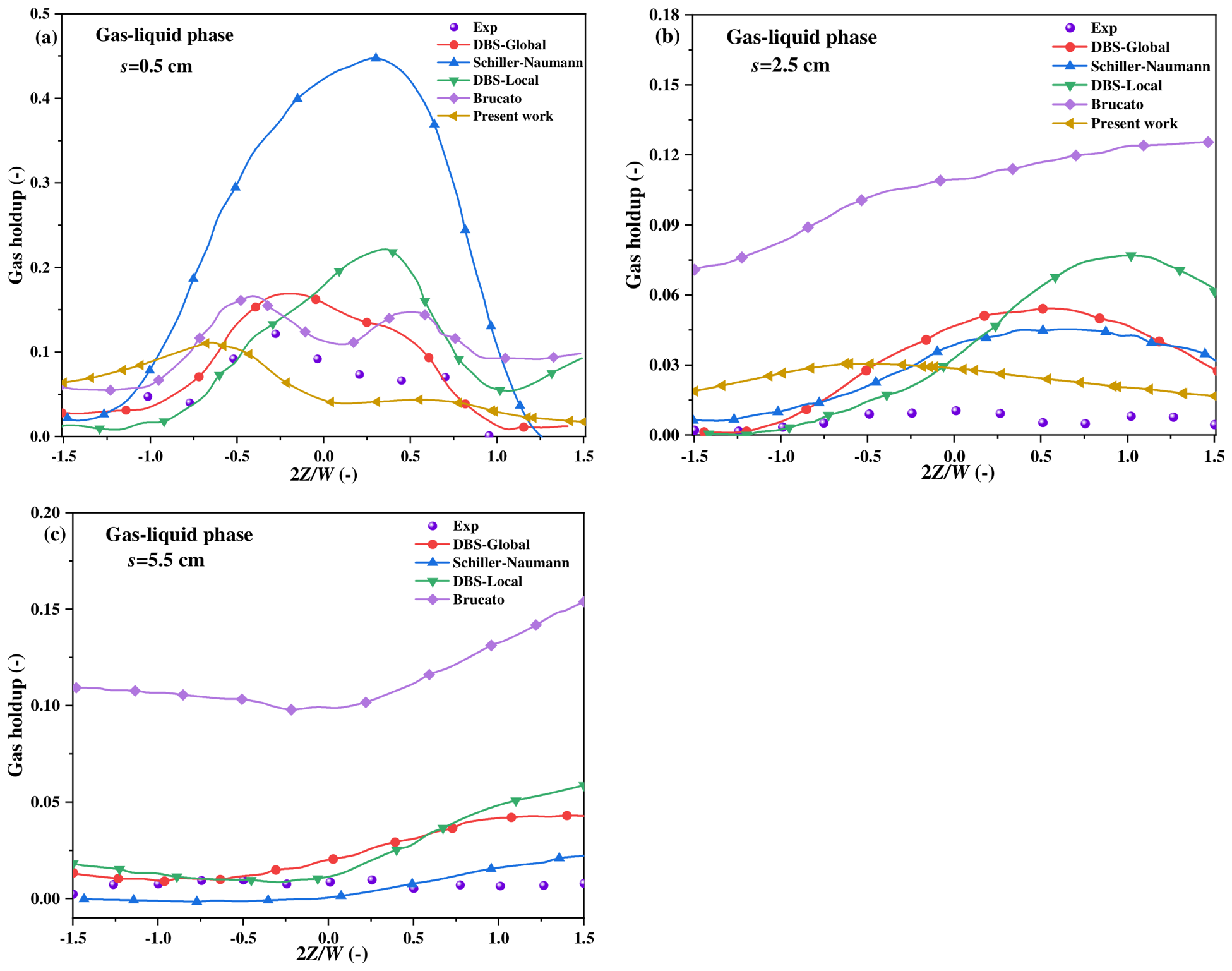
Similarly, Figure 5 compares the axial gas-holdup profiles at the same three radial positions. The different drag models generally capture the axial distribution of gas holdup in the impeller discharge region, although considerable discrepancies exist among the predictions, indicating the high sensitivity of gas holdup to the drag model. The different drag models generally capture the axial distribution of gas holdup in the impeller discharge region, although considerable discrepancies exist among the predictions, indicating the high sensitivity of gas holdup to the drag model. In comparison, the present simulation reasonably reproduces the experimentally observed gas holdup profiles. At s = 0.5 cm, the peak position of the gas holdup is well captured, although the gas holdup is slightly underestimated above the impeller disk. As the radial distance increases to s = 2.5 and 5.5 cm, the present simulation successfully reproduces the overall variation in gas holdup along the axial direction and remains in good agreement with the experimental measurements, with only minor local deviations.

4. Results and Discussion

4.1. Gas Holdup, Velocity Field, and Interphase Drag Coefficient Distribution

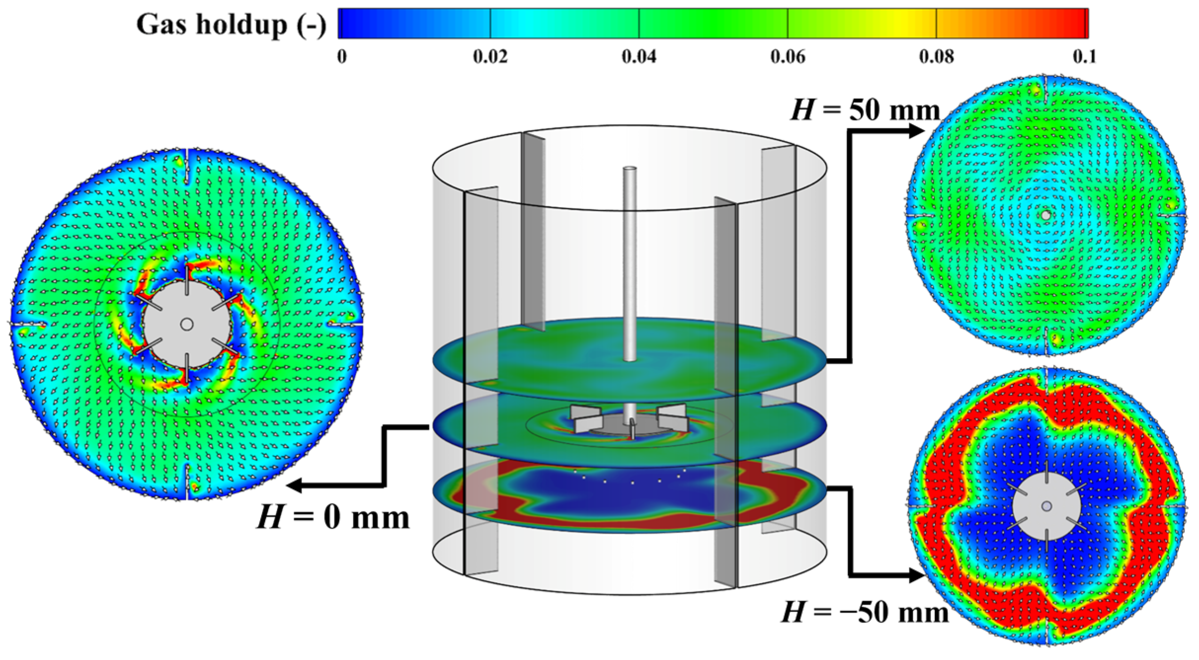
The gas holdup is the important indicator of gas dispersion in gas–liquid stirred tanks. Figure 6 shows the gas holdup distribution at three horizontal planes, namely H = −50 mm, 0 mm and 50 mm, with velocity vectors. At the impeller mid-plane (H = 0 mm), gas is distributed non-uniformly and a clear gas accumulation appears behind the impeller blades. This behavior is associated with the low-pressure regions and strong local shear generated by the Rushton turbine. Below the impeller (H = −50 mm), a continuous annular zone of high gas holdup forms near the outer region of the tank. The local circulation near the vessel wall inhibits the direct upward escape of bubbles and promotes gas accumulation in this lower region. Above the impeller (H = 50 mm), the combined effects of liquid circulation and bubble buoyancy lead to a more uniform gas distribution. Therefore, the gas holdup field reflects the competition between impeller-induced radial dispersion, buoyancy-driven bubble rise and circulation-controlled residence time.

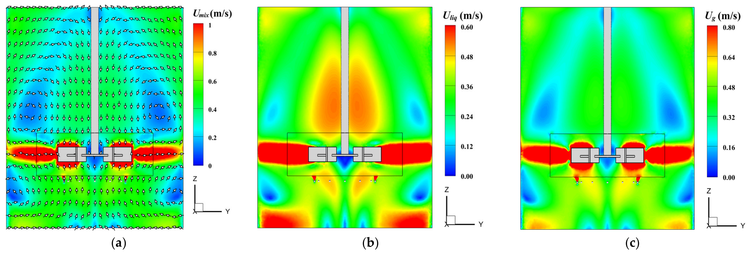
The velocity contour plots for the mixture phase (gas–liquid two-phase mixture), liquid phase, and gas phase in the cross-sectional plane (X = 0 mm) are depicted in Figure 7. The flow field demonstrates the characteristic pattern of a Rushton turbine, with the radial discharge of the impeller divided into upper and lower circulation zones, and the liquid returns axially to the top and bottom of the impeller (Figure 7a). Therefore, the liquid phase has a distinctly localized high-velocity region near the stirring shaft and the bottom of the tank. The overall velocity distributions of the mixture, liquid phase, and gas phase present similar characteristics featuring confined high-velocity zones adjacent to the impeller. The upper circulation vortex extends more widely than the lower counterpart, while low velocities occur at all four vortex cores. In addition, the liquid phase maintains higher velocities at these cores than the gas or mixture phases due to its greater inertia.

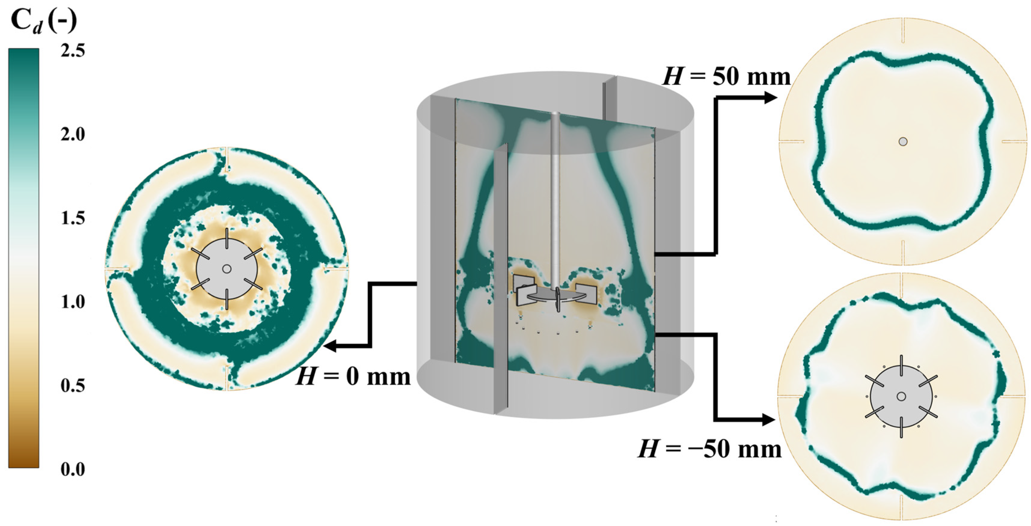
Figure 8 illustrates the distribution drag coefficient at cross-section X = 0 mm and the heights of −50 mm, 0 mm, and 50 mm. The relevant expressions for the drag coefficient are given by Equations (5) and (6). The high drag coefficient corresponds to a low Reynolds number, whereas a low Reynolds number indicates a small slip velocity between gas and liquid. In the cross-sectional X = 0 mm, the high drag coefficient is concentrated at the bottom and top of the vessel, the impeller discharge zone, as well as the four vortex core regions. This indicates that these regions have a small gas–liquid slip velocity and exhibit enhanced kinematic coupling between the dispersed gas phase and the continuous liquid phase. At the horizontal plane of the impeller (H = 0 mm), a continuous annular band of high drag coefficient aligns with the radial jet path, extending slightly beyond the blade tips toward the baffles. This arises from intense turbulence at blade tips, which promotes liquid pulsations that enhance bubble entrainment by the liquid phase and reduce slip velocity. Similar annular bands appear above (H = 50 mm) and below (H = −50 mm) the impeller but with markedly reduced extents, owing to the decay of turbulence intensity with vertical distance and the growing relative importance of buoyancy, which results in an increased slip velocity.

4.2. Effect of Stirring Speed

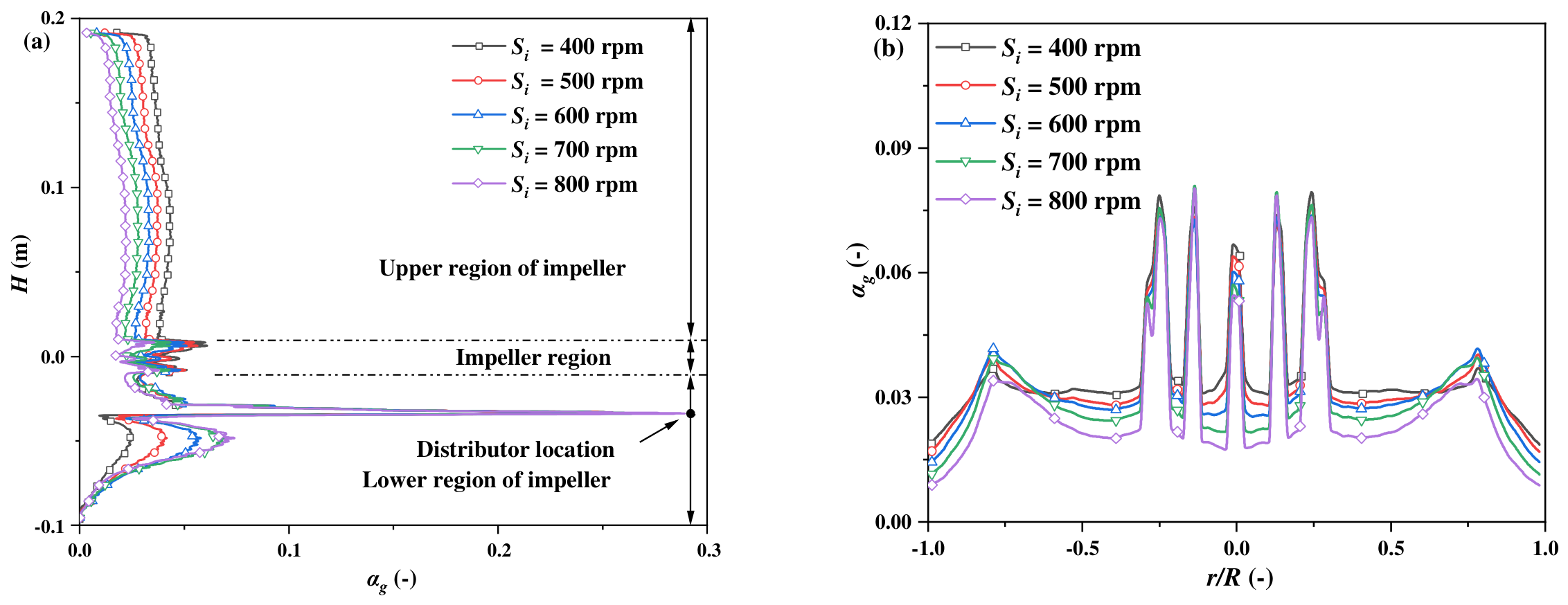
The effect of the stirring speed on the axial distribution of the gas holdup is exhibited in Figure 9a. At the position of the gas distributor, the gas holdup is significantly higher than in other regions. Under the stirring speed of 400 rpm, the pumping capacity of the impeller is insufficient to fully entrain bubbles into the lower circulation loop. As a result, bubbles mainly rise under buoyancy, and the gas holdup above the impeller is higher than that below the impeller. When the stirring speed increases from 400 to 800 rpm, the impeller discharge flow and local shear are strengthened. More gas is captured by the liquid circulation and transported downward into the lower region of the tank. This enhances gas redistribution, although the gas holdup in the upper regions decreases because the stronger circulation shortens the bubble residence time and accelerates gas escape through the degassing outlet. Figure 9b demonstrates the effect of stirring speed on the radial distribution of gas holdup. The radial distribution of gas holdup exhibits four obvious peaks in the impeller region (|r/R| ≤ 0.25), corresponding to the tips of the impeller blades, respectively. With increasing stirring speed, the radial gas holdup becomes slightly lower at most radial positions. This does not indicate weaker dispersion. Instead, it suggests that gas is distributed over a larger tank volume rather than being concentrated near the impeller. Therefore, stirring speed improves gas dispersion mainly by strengthening liquid circulation and redistributing bubbles through the impeller-induced flow loops.

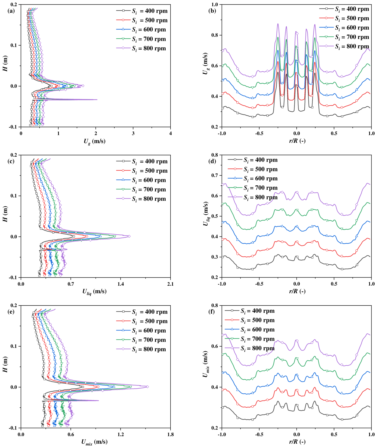
The resultant velocities of the gas, liquid and mixture phases under different stirring speeds are presented in Figure 10. In both axial and radial directions, all phase velocities increase as the stirring speed rises. This trend is expected because the impeller transfers more mechanical energy to the liquid phase, which then entrains the dispersed gas phase through interphase momentum exchange. The radial velocity field is especially important for Rushton turbines because radial discharge is the dominant flow mechanism. Near the impeller blade tips, the liquid velocity increases rapidly and drives bubbles outward. When bubbles follow the radial liquid jet, the local slip velocity is reduced, which is consistent with the high-drag-coefficient region observed near the impeller plane. The difference between gas and liquid velocities provides a physical explanation for the change in mixing performance. At low stirring speed, the liquid circulation is weak and bubbles are more strongly controlled by buoyancy, which increases the gas–liquid slip in regions away from the impeller. Under this condition, interphase coupling is insufficient and extensive low-velocity zones remain in the tank. As stirring speed increases, the liquid circulation becomes strong enough to entrain more bubbles into the circulation loops, improving the kinematic coupling between gas and liquid phases.

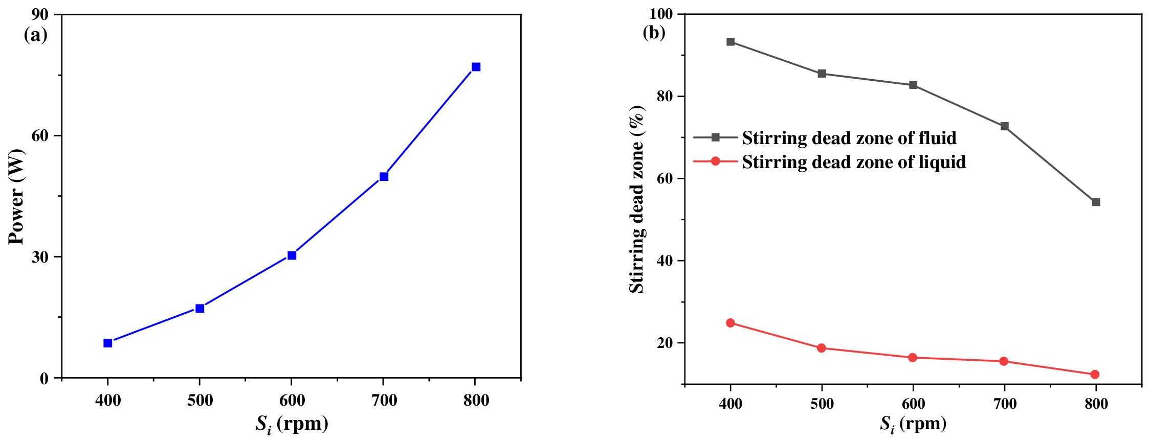
The effect of the stirring velocity on the stirring power, as well as the stirring dead zone of the liquid and fluid, is quantified in Figure 11. Increasing the stirring speed from 400 to 800 rpm reduces the mixture dead-zone fraction from 93.31% to 54.27% and the liquid dead-zone fraction from 24.64% to 12.08%. This confirms that stirring speed is the most direct operating parameter for suppressing stagnant zones. However, the corresponding power consumption increases sharply from 8.78 to 77.00 W. Therefore, increasing stirring speed improves mixing by strengthening radial discharge, reducing poorly mixed regions and enhancing drag-mediated gas–liquid coupling, but this improvement is achieved at a substantial energy cost. For practical operation, the optimum speed should therefore be selected from the balance between dead-zone suppression and power demand, rather than from maximum gas dispersion alone.

4.3. Effect of Gas Injection Velocity

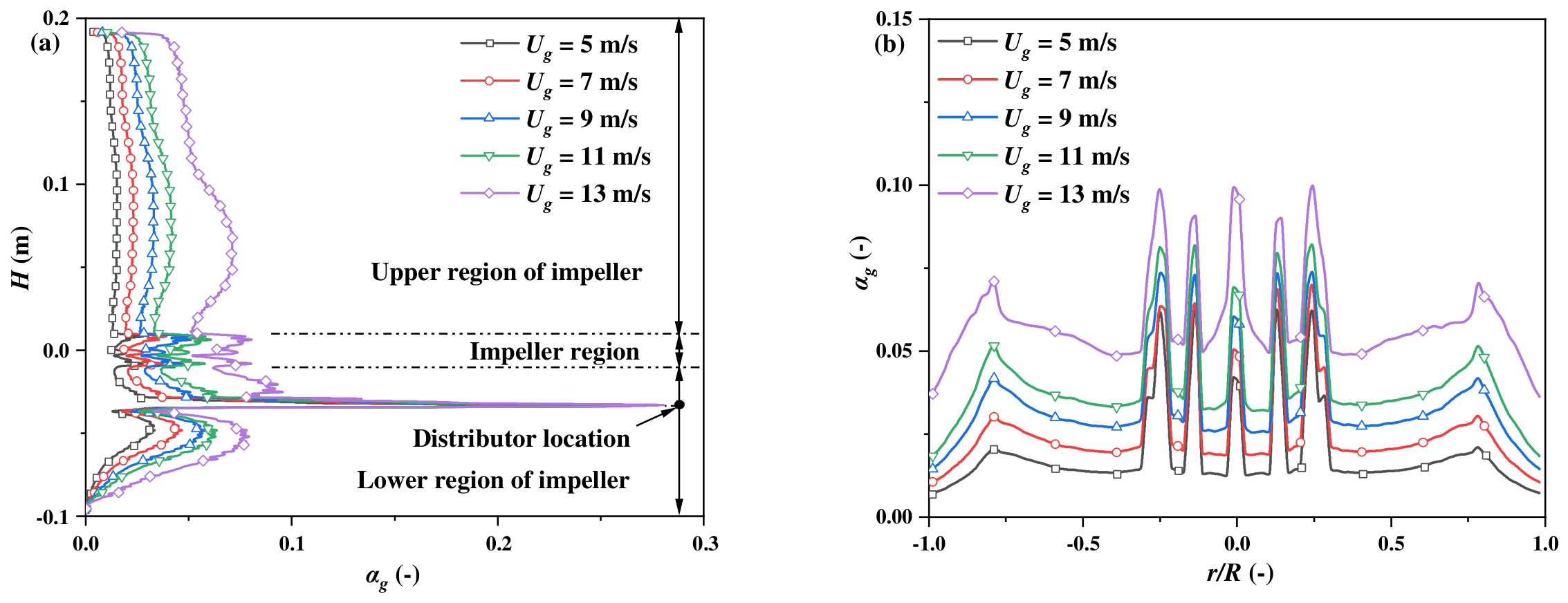
The effects of gas injection velocity on the axial and radial distributions of gas holdup are shown in Figure 12. As the gas injection velocity increases, the amount of gas introduced into the tank increases, leading to a higher overall gas holdup as more bubbles are transported into the impeller circulation region. However, the basic upper and lower circulation patterns induced by the impeller remain essentially unchanged. Under all gas injection velocities investigated, the axial gas holdup remains higher above the impeller than below it, indicating that buoyancy-driven upward bubble migration continues to play an important role in axial gas redistribution, even under high gas-loading conditions. At moderate gas injection velocities, bubbles can still be effectively entrained and redistributed by the impeller-driven liquid flow. At excessively high gas injection velocities; however, gas accumulation behind the impeller blades weakens the effective pumping capacity of the impeller and disturbs the radial liquid jet, preventing part of the injected gas from being effectively transported throughout the vessel. Consequently, although the axial and radial gas holdup generally increase at high gas injection velocities, the local gas holdup peaks and spatial gradients become more pronounced, indicating a deterioration in gas-distribution uniformity.

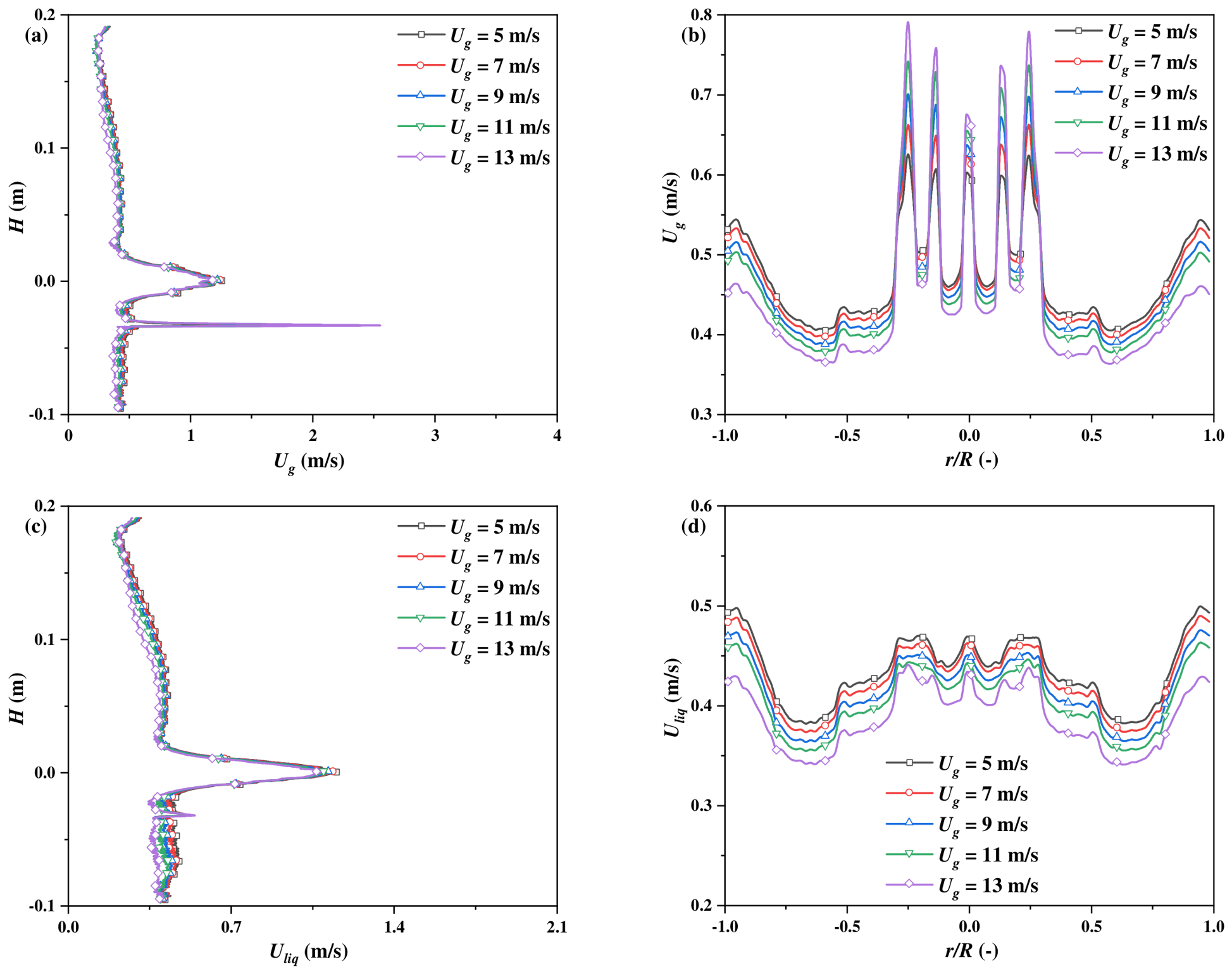
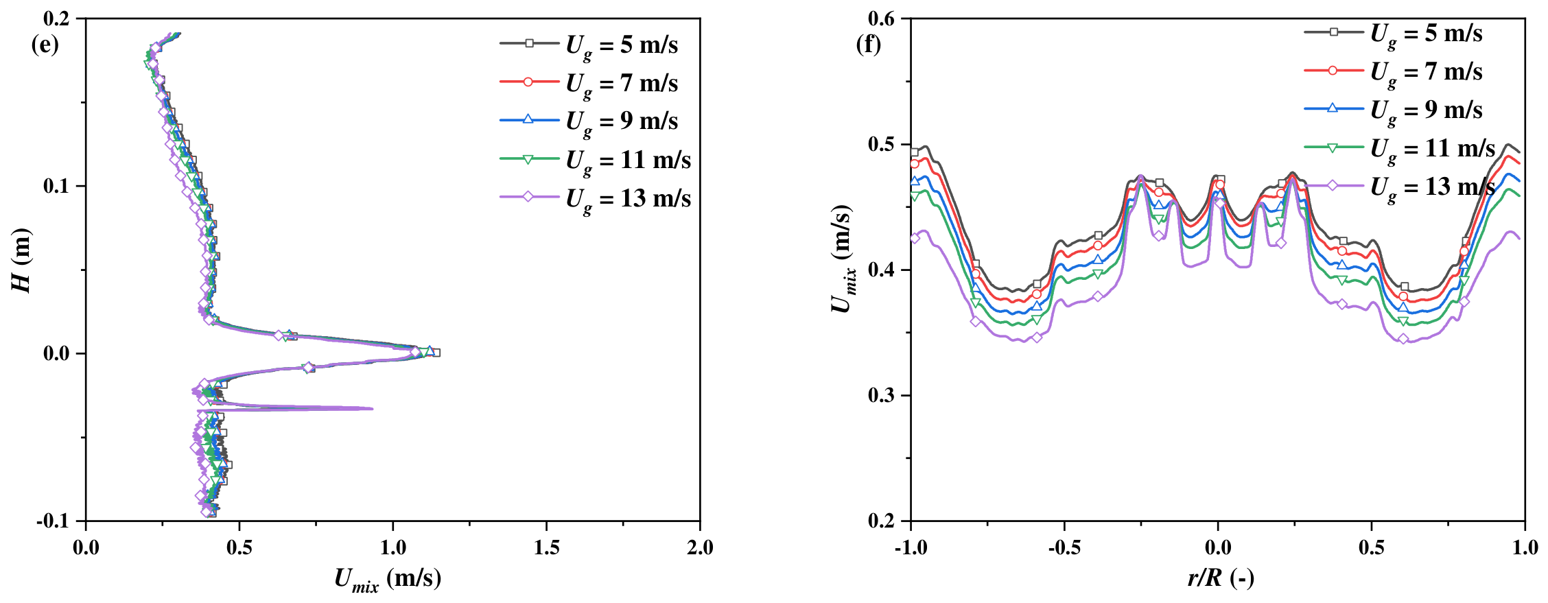
The impact of gas injection velocity on the resultant velocities of the gas, liquid, and mixture phases is presented in Figure 13. Since the impeller acts as the primary source of momentum in the stirred tank, variations in gas injection velocity have only a limited influence on the axial velocity distributions of the three phases. In the radial direction, however, the liquid and mixture velocities generally decrease with increasing gas injection velocity, whereas the gas velocity increases near the impeller but decreases in regions away from it. This behavior indicates that excessive gas loading weakens the effective pumping capacity of the impeller and suppresses liquid-phase circulation. Although the gas velocity increases locally in the impeller region because of the higher gas throughput and blade-induced shear, the liquid phase becomes less capable of entraining and redistributing the injected bubbles. Consequently, the mismatch between gas motion and liquid circulation increases the local gas–liquid slip velocity in parts of the tank and weakens effective interphase momentum transfer.

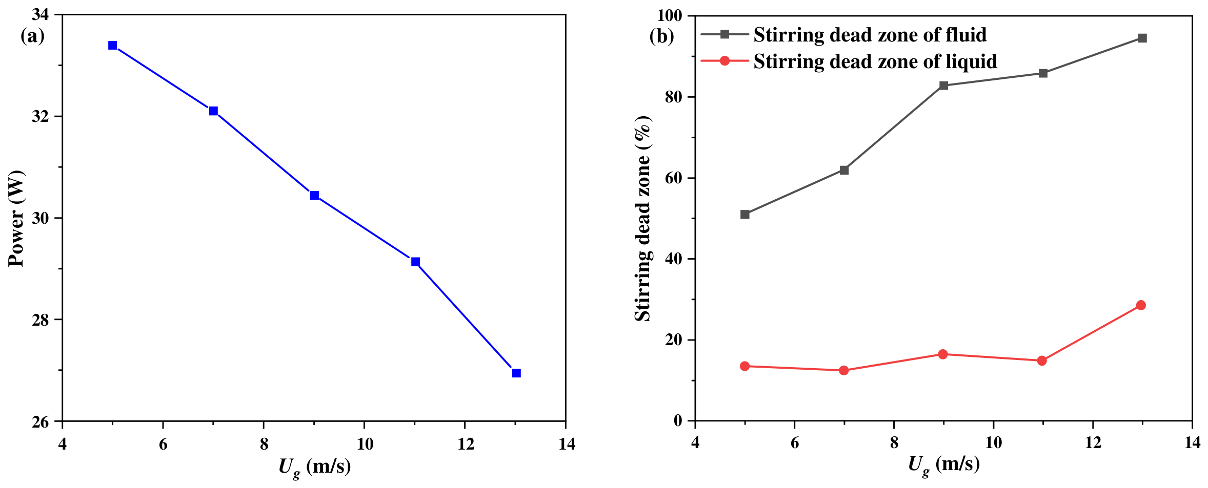
The effect of the gas injection velocity on the stirring power, as well as the stirring dead zone of the liquid and fluid, is illustrated in Figure 14. As shown in Figure 14a, with the increase in gas injection velocity, the agitation power decreases from 33.3 W to 26.9 W due to the reduction in impeller rotational resistance. The enhanced gas injection velocity impedes the liquid phase circulatory flow, thus expanding the stirring dead zone of the fluid, which increases from 50.94% to 94.54%. However, with the increase in gas injection velocity (5–13 m/s), the stirring dead zone of liquid develops fluctuating variations. When the gas injection velocity is increased from 5 m/s to 7 m/s, the gas is effectively dispersed by the impeller while creating a favorable turbulent effect on the liquid phase, reducing the stirring dead zone from 13.21% to 12.13%. Conversely, when the gas injection velocity is raised from 7 m/s to 13 m/s, gas accumulates behind the impeller blades to form gas cavities, which reduces the pumping efficiency of the impeller and consequently increases the stirring dead zone from 12.13% to 28.32%.

4.4. Effect of Blade Length

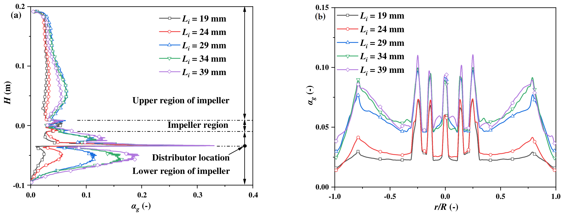
The effect of blade length on the axial and radial distributions of gas holdup is shown in Figure 15. Increasing the blade length enlarges the swept area of the impeller and enhances its radial discharge capacity, thereby strengthening liquid circulation and promoting bubble entrainment and redistribution within the tank. As a result, the gas holdup generally increases in both the axial and radial directions. For different blade lengths, the variation in gas holdup is more pronounced in the region below the impeller than above it, and the axial profiles show that the lower region maintains a higher gas holdup. This behavior is closely associated with the position of the gas distributor below the impeller and the strengthened lower circulation loop induced by longer blades. A larger blade length improves the ability of the radial jet to entrain bubbles from the distributor region and transport them into the lower circulation zone, making the gas holdup below the impeller more sensitive to blade length. When the blade length reaches 39 mm, however, the increase in axial gas holdup becomes less evident, particularly in the region above the impeller. A similar weakening of the increasing trend is also observed in the radial distribution. This suggests that the improvement in gas dispersion becomes marginal beyond a certain blade length. Under a fixed rotational speed, further increasing the blade length lead to a rapid rise in power consumption, whereas the enhancement of circulation and gas retention does not increase proportionally. Therefore, although increasing blade length is effective in improving gas holdup and bubble redistribution, an excessively long blade may result in diminishing returns because of the increased power demand and limited additional improvement in liquid circulation.

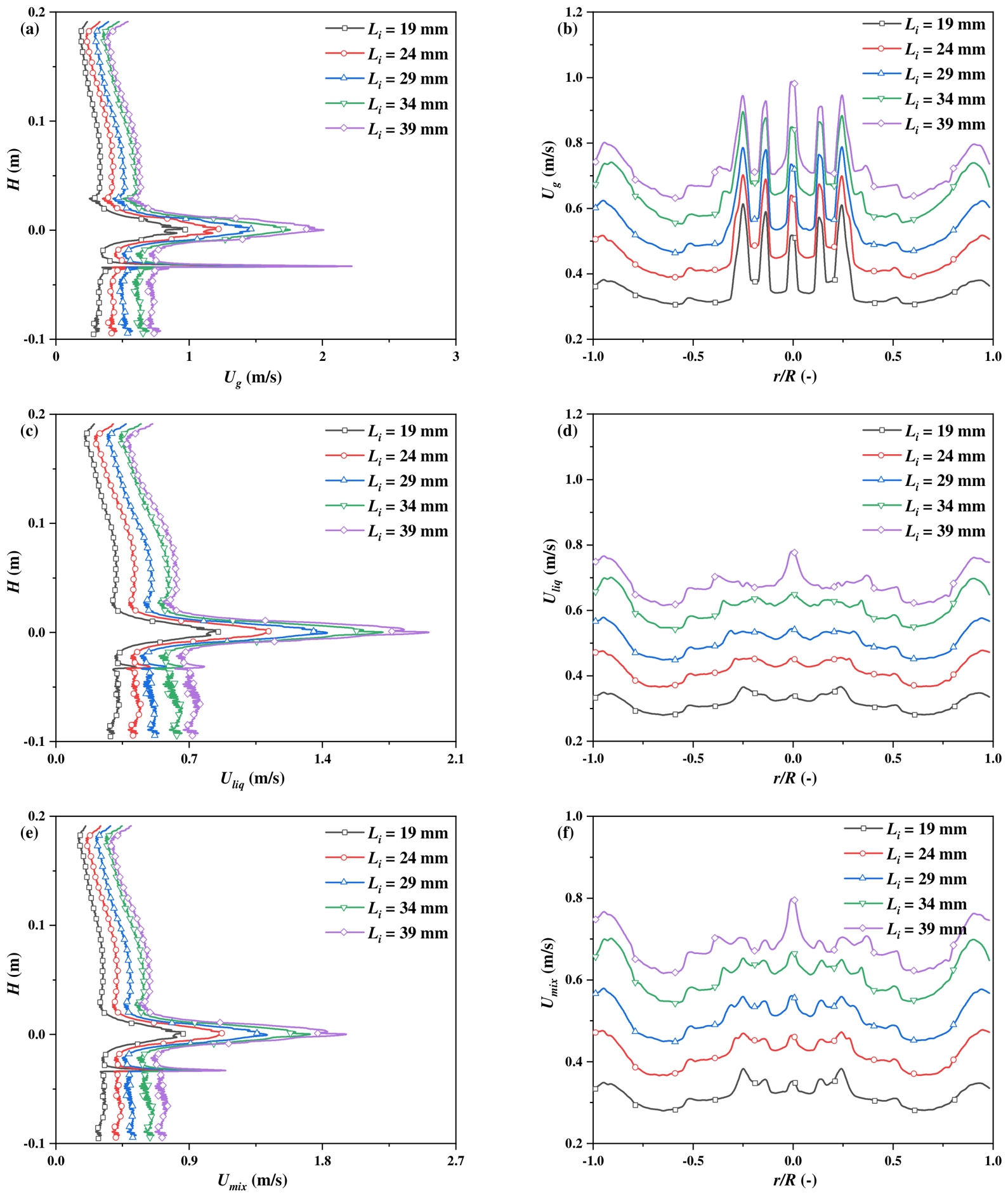
Figure 16 presents the effect of blade length on the axial and radial distributions of the resultant velocities of the gas phase, liquid phase, and mixture phase. Increasing the blade length increases the velocities of all three phases in both the axial and radial distributions. The increase in the radial velocity is particularly important because it strengthens the primary discharge flow generated by the impeller. The stronger liquid jet entrains bubbles more effectively and helps reduce local gas–liquid slip in the discharge region. As a result, drag-mediated phase coupling is enhanced, and the transport of gas from the impeller zone to the bulk liquid is promoted. At the largest blade length, however, the increasing trend of the phase velocities becomes weaker. This suggests that, under a fixed rotational speed, the hydrodynamic system gradually approaches a saturation-like condition, where further increases in blade length provide only limited additional enhancement of phase transport.

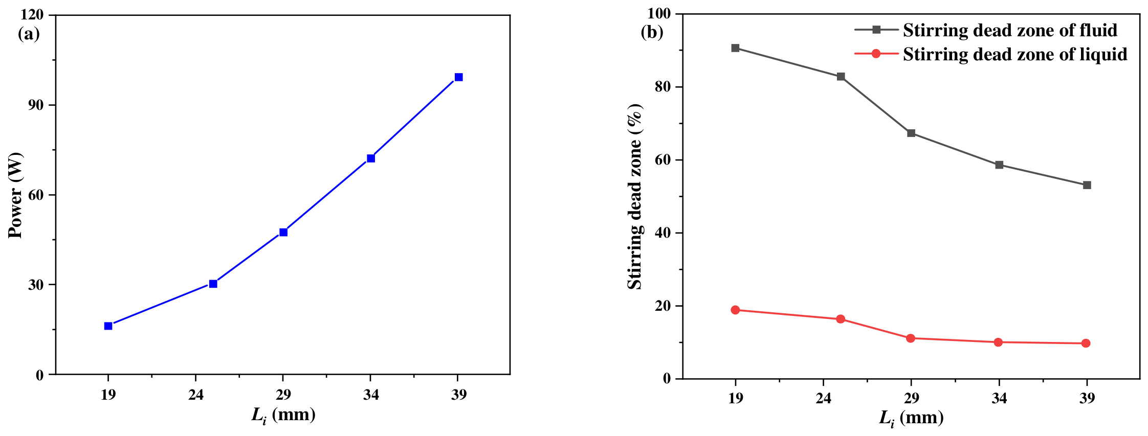
Figure 17a shows the effect of blade length on power consumption. As the blade length increases, the power consumption rises markedly from 16.46 to 99.25 W. This increase can be attributed to the enlarged blade-swept area and stronger radial discharge flow, which increase the hydrodynamic resistance. Figure 17b presents the corresponding variation in the dead-zone fractions of the mixture and liquid phases. Increasing blade length significantly reduces the mixture-phase dead-zone fraction from 90.63% to 53.07% and the liquid-phase dead-zone fraction from 18.66% to 9.50%. This indicates that longer blades can strengthen liquid circulation, enhance bubble entrainment and redistribution, and improve the overall mixing state in the tank. However, the improvement becomes marginal when the blade length is further increased from 34 to 39 mm, as the liquid-phase dead-zone fraction decreases only slightly from 9.77% to 9.50%. Therefore, although increasing blade length is an effective strategy for suppressing dead zones, its benefit is accompanied by a substantial power penalty and clear diminishing returns at excessive blade length. For the present Rushton turbine stirred tank, blade length is more effective than blade height in enhancing global circulation, but an excessively long blade is not necessarily energy-efficient.

4.5. Effect of Blade Height

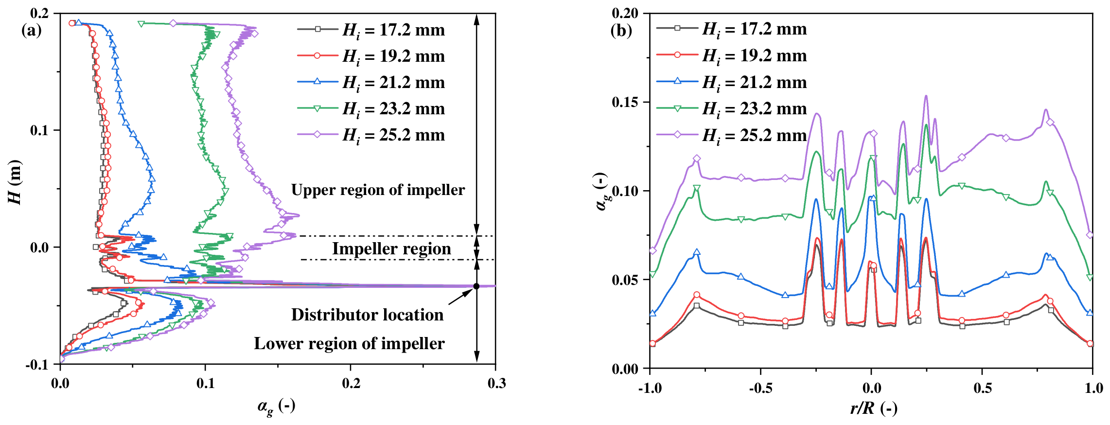
The effects of impeller blade height on the axial and radial distributions of gas holdup are shown in Figure 18a and Figure 18b, respectively. As the blade height of the impeller increases from 17.2 to 25.2 mm, the gas holdup generally increases in both the axial and radial directions. This is because increased blade height prolongs bubble circulation paths via an expanded scope of upper and lower dual circulation loops inside the vessel, which extends the bubble residence time and thus elevates the gas holdup. In the axial direction, the gas holdup in the lower region of the impeller increases only slightly with increasing blade height, whereas a more pronounced increase is observed near and above the impeller. The fluctuations around the impeller region can be attributed to the blade wakes, trailing vortices, and strong local shear generated by the rotating blades. When the blade height increases to 23.2 and 25.2 mm, the gas holdup in the upper region becomes higher than that in the lower region, suggesting that the enlarged blade surface strengthens the radial discharge flow and promotes the upper circulation formed after wall impingement. As a result, more bubbles are entrained from the impeller region and redistributed into the upper part of the tank. By contrast, at smaller blade heights, the weaker pumping and entrainment capacity limits bubble transport toward the upper and peripheral regions, resulting in less effective redistribution of gas holdup. The radial distribution further shows that increasing blade height raises the gas holdup over most radial positions, with a more evident increase away from the impeller region. Consequently, the gas holdup gradient between the impeller region and the peripheral region is reduced, indicating an expanded bubble dispersion range and a more uniform radial gas distribution.

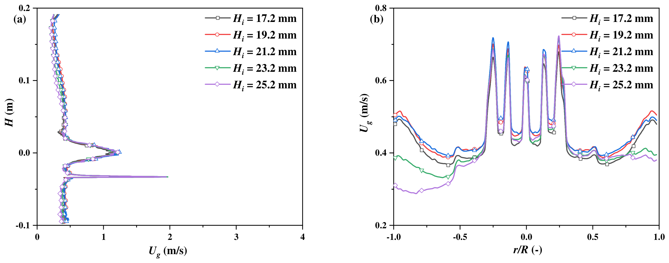
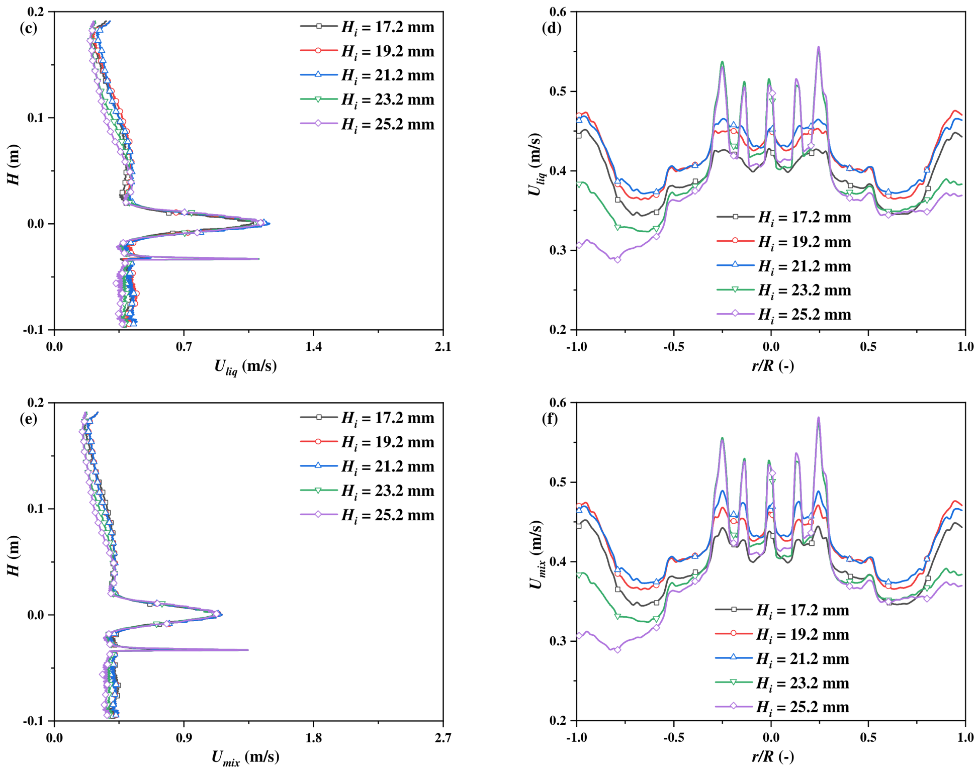
The effect of blade height on the resultant velocities of the gas, liquid, and mixture phases is exhibited in Figure 19. The phase velocity distributions indicate that increasing blade height mainly modifies the local flow field around the impeller and along the radial discharge path, rather than fundamentally altering the tank-scale circulation pattern. In the axial direction, the velocities of the gas, liquid, and mixture phases vary only slightly with blade height, suggesting that a taller blade does not substantially improve the overall pumping capacity of the Rushton turbine under the present operating conditions. More noticeable variations are observed in the radial velocity profiles, particularly in the impeller discharge region and toward the peripheral part of the tank. This behavior can be attributed to the increased blade surface area, which enhances local shear and modifies gas–liquid interaction in the blade-swept region. A larger blade height can promote local bubble entrainment by the impeller-driven liquid flow, thereby reducing the gas–liquid slip velocity in regions where bubbles are effectively captured and transported with the liquid phase. The reduced local slip velocity strengthens phase coupling and helps improve gas holdup uniformity around the impeller. However, because the radial discharge range and the global circulation loops are not significantly expanded, the influence of blade height on tank-scale circulation remains limited compared with that of blade length.

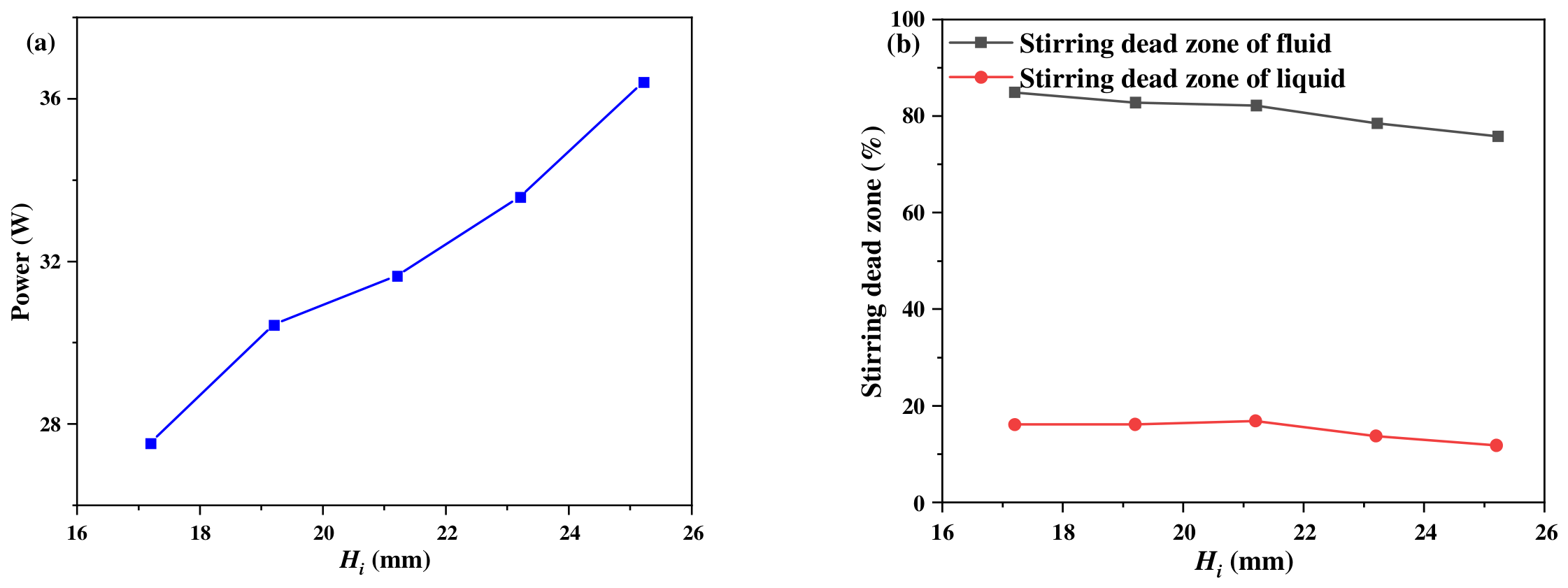
Figure 20a illustrates the effect of blade height on power consumption. As the blade height increases, the projected area of the impeller blade exposed to the liquid becomes larger, thereby increasing the hydrodynamic resistance and the torque required to drive the impeller. Consequently, the stirring power increases from 27.55 to 36.39 W. Figure 20b shows the corresponding effect of blade height on the dead-zone fractions of the mixture and liquid phases. With increasing blade height, the mixture-phase dead-zone fraction decreases from 84.89% to 75.83%, while the liquid-phase dead-zone fraction decreases from 16.10% to 11.81%. Although this reduction is beneficial for mixing, the improvement is relatively limited compared with that achieved by increasing the stirring speed or blade length. This result indicates that increasing blade height mainly enhances local shear and gas–liquid interaction near the impeller, but does not substantially expand the radial discharge range or strengthen the tank-scale circulation loops. Therefore, increasing blade height can improve local gas dispersion and moderately reduce the dead zone, but it is not the most effective strategy for global mixing enhancement in the present Rushton turbine stirred tank.

5. Conclusions

In this study, a Euler–Euler two-fluid model coupled with the standard k–ε turbulence model was adopted to investigate gas dispersion, interphase drag coefficient characteristics, power consumption, and the evolution of mixing dead zones in a baffled Rushton-turbine stirred tank. Detailed numerical simulations fully elucidate the dynamic evolution patterns of hydrodynamic behaviors inside the system. The influences of stirring speed, gas injection velocity, blade height and blade length were systematically analyzed. The main conclusions are summarized as follows:

(1)

The baseline flow field shows that gas dispersion in the stirred tank is governed by the combined effects of impeller-induced radial discharge, buoyancy-driven bubble rise, and circulation-controlled residence time. High drag-coefficient regions are mainly located along the impeller discharge path, near vortex-core regions, and in annular structures close to the vessel wall. These regions correspond to relatively small gas–liquid slip velocities and stronger kinematic coupling between the dispersed gas phase and the continuous liquid phase.

(2)

Increasing stirring speed is the most direct operating strategy for enhancing liquid circulation and suppressing stagnant zones. As the stirring speed increases from 400 to 800 rpm, the mixture-phase dead-zone fraction decreases from 93.31% to 54.27%, and the liquid-phase dead-zone fraction decreases from 24.64% to 12.08%. This improvement is caused by stronger radial discharge, enhanced bubble entrainment, and improved drag-mediated gas–liquid coupling. However, the corresponding power consumption increases sharply from 8.78 to 77.00 W. Therefore, increasing stirring speed improves mixing performance effectively, but this enhancement is accompanied by a substantial energy penalty.

(3)

Increasing gas injection velocity raises the overall gas holdup but does not necessarily improve mixing performance. As the gas injection velocity increases from 5 to 13 m/s, the power consumption decreases from 33.3 to 26.9 W, while the mixture-phase dead-zone fraction increases from 50.94% to 94.54%. The liquid-phase dead-zone fraction exhibits a non-monotonic response, decreasing slightly from 13.21% to 12.13% between 5 and 7 m/s and then increasing to 28.32% at 13 m/s. This behavior indicates that moderate aeration can provide limited enhancement of local liquid agitation, whereas excessive gas loading promotes gas accumulation near the impeller, weakens its effective pumping capacity, and suppresses liquid circulation.

(4)

Blade height mainly regulates local shear and gas–liquid interaction near the impeller. Increasing the blade height from 17.2 to 25.2 mm increases the power consumption from 27.55 to 36.39 W, while the mixture-phase and liquid-phase dead-zone fractions decrease from 84.89% to 75.83% and from 16.10% to 11.81%, respectively. Although a larger blade height improves local gas redistribution and radial gas-holdup uniformity, its effect on tank-scale circulation and global dead-zone suppression remains limited. Therefore, blade height should be regarded as a local flow-regulation parameter rather than the dominant parameter for global mixing enhancement.

(5)

Blade length is the most effective geometric parameter for reducing dead zones in the present Rushton-turbine stirred tank. Increasing the blade length from 19 to 39 mm strengthens the radial discharge flow and bubble redistribution, reducing the mixture-phase dead-zone fraction from 90.63% to 53.07% and the liquid-phase dead-zone fraction from 18.66% to 9.50%. However, the power consumption increases markedly from 16.46 to 99.25 W. Moreover, the reduction in the liquid-phase dead zone becomes marginal when the blade length increases from 34 to 39 mm, indicating diminishing returns at excessive blade length. Therefore, blade length is more effective than blade height for enhancing global circulation, but an excessively long blade is not necessarily energy-efficient.

Overall, the results demonstrate that gas–liquid mixing in a Rushton-turbine stirred tank should be evaluated through the coupled relationship among gas holdup, phase velocity, interphase drag, power consumption, and dead-zone fraction. For energy-efficient operation, simply maximizing gas holdup or reducing power draw is insufficient. A practical design should balance gas dispersion, liquid circulation, and power consumption, with stirring speed and blade length being the dominant control parameters, while gas injection velocity and blade height should be optimized to avoid gas accumulation and inefficient energy use.

References

1. Zhao, Z.; Chen, F.; Liu, J.; Liu, Q.; Hou, Y.; Yang, N.; Xie, G. Numerical simulation study of gas-liquid two-phase flow in a pressurized leaching stirred tank. Processes 2024, 12, 896. [Google Scholar] [CrossRef] [Scilit]
2. Cudak, M.; Rakoczy, R. Hydrodynamics of gas-liquid and biophase-gas-liquid systems in stirred tanks of different scales. Korean J. Chem. Eng. 2022, 39, 2959–2971. [Google Scholar] [CrossRef] [Scilit]
3. Montante, G.; Paglianti, A. Gas hold-up distribution and mixing time in gas–liquid stirred tanks. Chem. Eng. J. 2015, 279, 648–658. [Google Scholar] [CrossRef] [Scilit]
4. Liu, B.; Xiao, Q.; Sun, N.; Gao, P.; Fan, F.; Sunden, B. Effect of gas distributor on gas–liquid dispersion and mass transfer characteristics in stirred tank. Chem. Eng. Res. Des. 2019, 145, 314–322. [Google Scholar] [CrossRef] [Scilit]
5. Ngoma, E.; Pakostova, E.; Wiesner, J.A.; Clark, T.; Laamanen, C.; Mykytczuk, N. Commissioning and Optimization of Pilot-Scale Stirred Tank Reactors in Biohydrometallurgy. J. Sustain. Metall. 2025, 11, 3806–3822. [Google Scholar] [CrossRef] [Scilit]
6. Voinov, N.A.; Frolov, A.S.; Bogatkova, A.V.; Zemtsov, D.A.; Zhukova, O.P. Method for intensive gas–liquid dispersion in a stirred tank. ChemEngineering 2023, 7, 30. [Google Scholar] [CrossRef] [Scilit]
7. Zhang, Q.; Yong, Y.; Mao, Z.-S.; Yang, C.; Zhao, C. Experimental determination and numerical simulation of mixing time in a gas–liquid stirred tank. Chem. Eng. Sci. 2009, 64, 2926–2933. [Google Scholar] [CrossRef] [Scilit]
8. Amiraftabi, M.; Khiadani, M.; Mohammed, H.A.; Arshad, A. CFD-PBM and experimental investigation of a shear thinning fluid in a gas-liquid tank agitated by a helical ribbon impeller. Sep. Purif. Technol. 2021, 272, 118855. [Google Scholar] [CrossRef] [Scilit]
9. Liu, L.; Chen, Z.-b.; Yan, H.-j.; Zhang, D.-k.; Zhou, P. Numerical simulation and multi-objective parameter optimization of gas−liquid flow in horizontal stirred tank. Trans. Nonferrous Met. Soc. China 2023, 33, 958–968. [Google Scholar] [CrossRef] [Scilit]
10. Li, L.; Chen, C.; Tao, X.; Qi, H.; Liu, T.; Yan, Q.; Deng, F.; Allayev, A.; Lin, W.; Wang, J. Effect of Salt Solution Tracer Dosage on the Transport and Mixing of Tracer in a Water Model of Asymmetrical Gas-Stirred Ladle with a Moderate Gas Flowrate. Symmetry 2024, 16, 619. [Google Scholar] [CrossRef] [Scilit]
11. Zhao, Y.; Chen, C.; Li, L.; Wang, T.; Chen, L.; Wang, J. Application of an Improved Tracer in a Water Model of Ladle. Metall. Mater. Trans. B Process Metall. Mater. Process. Sci. 2025, 56, 6725–6745. [Google Scholar] [CrossRef] [Scilit]
12. Rong, Z.; Hou, D.; Chen, C.; Song, G.; Du, Z.; Li, J.; Zhang, H.; Lin, W.; Chen, L.; Qian, G. The Effect of Baffle Structure and Rotational Speed on the Flow Field in the Silicon Purification Process via the Rotational Segregation Method: A Water Model Study on Tracer Transport and Concentration Variation. Processes 2026, 14, 1500. [Google Scholar] [CrossRef] [Scilit]
13. Gu, D.; Wen, L.; Xu, H.; Ye, M. Study on hydrodynamics characteristics in a gas-liquid stirred tank with a self-similarity impeller based on CFD-PBM coupled model. J. Taiwan Inst. Chem. Eng. 2023, 143, 104688. [Google Scholar] [CrossRef] [Scilit]
14. Maluta, F.; Paglianti, A.; Montante, G. Prediction of gas cavities size and structure and their effect on the power consumption in a gas-liquid stirred tank by means of a two-fluid RANS model. Chem. Eng. Sci. 2021, 241, 116677. [Google Scholar] [CrossRef] [Scilit]
15. Petitti, M.; Vanni, M.; Marchisio, D.L.; Buffo, A.; Podenzani, F. Simulation of coalescence, break-up and mass transfer in a gas–liquid stirred tank with CQMOM. Chem. Eng. J. 2013, 228, 1182–1194. [Google Scholar] [CrossRef] [Scilit]
16. Lane, G.; Schwarz, M.; Evans, G. Predicting gas–liquid flow in a mechanically stirred tank. Appl. Math. Model. 2002, 26, 223–235. [Google Scholar] [CrossRef] [Scilit]
17. Krýsa, P.; Kuhn, S.; Šoóš, M. Modelling of bubble breakage and coalescence in stirred and sparged bioreactor using the Euler–Lagrange approach coupled with volume of fluid method. Int. J. Heat Mass Transf. 2025, 252, 127249. [Google Scholar] [CrossRef] [Scilit]
18. Maluta, F.; Alberini, F.; Paglianti, A.; Montante, G. Hydrodynamics, power consumption and bubble size distribution in gas-liquid stirred tanks. Chem. Eng. Res. Des. 2023, 194, 582–596. [Google Scholar] [CrossRef] [Scilit]
19. Yan, Y.; Mohanarangam, K.; Yang, W.; Tu, J. Experimental measuring techniques for industrial-scale multiphase flow problems. Exp. Comput. Multiph. Flow 2024, 6, 1–13. [Google Scholar] [CrossRef] [Scilit]
20. Płusa, T.; Talaga, J.; Duda, A.; Duda, P. Modeling mixing dynamics in uncovered baffled and unbaffled stirred tanks. AIChE J. 2021, 67, e17322. [Google Scholar] [CrossRef] [Scilit]
21. Simon, E.; Augier, F.; Morchain, J.; Pierson, J.-L.; Liné, A. Investigation of the local apparent viscosity in a stirred tank with a shear-thinning fluid through particle image velocimetry. Chem. Eng. Res. Des. 2024, 206, 378–385. [Google Scholar] [CrossRef] [Scilit]
22. Ciou, Z.-Y.; Wu, C.Y. Investigation of the flow patterns and mixing efficiency in a stirred tank through particle image velocimetry. J. Taiwan Inst. Chem. Eng. 2023, 149, 104988. [Google Scholar] [CrossRef] [Scilit]
23. Story, A.; Jaworski, Z.; Simmons, M.J.; Nowak, E. Comparative PIV and LDA studies of Newtonian and non-Newtonian flows in an agitated tank. Chem. Pap. 2018, 72, 593–602. [Google Scholar] [CrossRef] [Scilit]
24. Kolano, M.; Kraume, M. A PIV study to quantify the relationships between viscoelasticity and flow behavior in stirred tanks. Chem. Eng. Sci. 2023, 282, 119301. [Google Scholar] [CrossRef] [Scilit]
25. Aubin, J.; Le Sauze, N.; Bertrand, J.; Fletcher, D.F.; Xuereb, C. PIV measurements of flow in an aerated tank stirred by a down- and an up-pumping axial flow impeller. Exp. Therm. Fluid. Sci. 2004, 28, 447–456. [Google Scholar] [CrossRef] [Scilit]
26. Schäfer, M.; Höfken, M.; Durst, F. Detailed LDV measurements for visualization of the flow field within a stirred-tank reactor equipped with a Rushton turbine. Chem. Eng. Res. Des. 1997, 75, 729–736. [Google Scholar] [CrossRef] [Scilit]
27. Benayad, S.; Salem, A.; Legrand, J. Investigation of the interaction of velocity and concentration fields by coupling LDV to conductivity probe in a continuous stirred tank reactor (CSTR). Chem. Eng. J. 2001, 84, 239–245. [Google Scholar] [CrossRef] [Scilit]
28. Wang, B.; Dai, J.; Yu, J.; Gao, X. Coupling superquadric Discrete Element Method-Computational Fluid Dynamics (DEM-CFD) with immersed boundary method for particle-resolved direct numerical simulations of non-spherical particle suspension and fluidisation. J. Fluid. Mech. 2025, 1019, A35. [Google Scholar] [CrossRef] [Scilit]
29. Gorji, M.; Bozorgmehry Boozarjomehry, R.; Kazemeini, M. CFD Modeling of gas-liquid hydrodynamics in a stirred tank reactor. Iran. J. Chem. Chem. Eng. 2007, 26, 85–96. [Google Scholar] [CrossRef]
30. Sajjadi, B.; Raman, A.A.A.; Ibrahim, S.; Shah, R.S.S.R.E. Review on gas-liquid mixing analysis in multiscale stirred vessel using CFD. Rev. Chem. Eng. 2012, 28, 171–189. [Google Scholar] [CrossRef] [Scilit]
31. Xia, Y.; Lin, Z.; Yu, Z. Modelling mesoscale turbulence in clustered gas–solid flows based on particle-resolved simulation data. J. Fluid Mech. 2025, 1021, A6. [Google Scholar] [CrossRef] [Scilit]
32. Liu, Y.-J.; Li, W.; Han, L.-C.; Cao, Y.; Luo, H.-a.; Al-Dahhan, M.; Dudukovic, M. γ-CT measurement and CFD simulation of cross section gas holdup distribution in a gas–liquid stirred standard Rushton tank. Chem. Eng. Sci. 2011, 66, 3721–3731. [Google Scholar] [CrossRef] [Scilit]
33. Li, Y.; Wang, J.; Lu, C.; Wang, S.; Dong, H. Gas–liquid flow characteristics and performance optimization of industrial downflow jet loop reactor based on computational fluid dynamics. Korean J. Chem. Eng. 2024, 41, 1637–1656. [Google Scholar] [CrossRef] [Scilit]
34. Ochieng, A.; Onyango, M.; Kiriamiti, K. Experimental measurement and computational fluid dynamics simulation of mixing in a stirred tank: A review. South Afr. J. Sci. 2009, 105, 421–426. [Google Scholar] [CrossRef] [Scilit]
35. Joshi, J.B.; Nere, N.K.; Rane, C.V.; Murthy, B.; Mathpati, C.S.; Patwardhan, A.W.; Ranade, V.V. CFD simulation of stirred tanks: Comparison of turbulence models. Part I: Radial flow impellers. Can. J. Chem. Eng. 2011, 89, 23–82. [Google Scholar] [CrossRef] [Scilit]
36. Joshi, J.B.; Nere, N.K.; Rane, C.V.; Murthy, B.; Mathpati, C.S.; Patwardhan, A.W.; Ranade, V.V. CFD simulation of stirred tanks: Comparison of turbulence models (Part II: Axial flow impellers, multiple impellers and multiphase dispersions). Can. J. Chem. Eng. 2011, 89, 754–816. [Google Scholar] [CrossRef] [Scilit]
37. Jahoda, M.; Tomášková, L.; Moštěk, M. CFD prediction of liquid homogenisation in a gas–liquid stirred tank. Chem. Eng. Res. Des. 2009, 87, 460–467. [Google Scholar] [CrossRef] [Scilit]
38. Duguay, J.; Lacey, J.; Massé, A. Evaluating the Euler-Euler approach for predicting a strongly 3D bubble-induced recirculatory flow with OpenFOAM. Chem. Eng. Sci. 2021, 229, 115982. [Google Scholar] [CrossRef] [Scilit]
39. Shi, P.; Rzehak, R. Bubbly flow in stirred tanks: Euler-Euler/RANS modeling. Chem. Eng. Sci. 2018, 190, 419–435. [Google Scholar] [CrossRef] [Scilit]
40. Tamburini, A.; Brucato, A.; Ciofalo, M.; Gagliano, G.; Micale, G.; Scargiali, F. CFD simulations of early-to fully-turbulent conditions in unbaffled and baffled vessels stirred by a Rushton turbine. Chem. Eng. Res. Des. 2021, 171, 36–47. [Google Scholar] [CrossRef] [Scilit]
41. Xu, C.; Liu, X.; Ding, C.; Zhou, X.; Xu, Y.; Gu, X. Power consumption and oxygen transfer optimization for C5 sugar acid production in a gas-liquid stirred tank bioreactor using CFD-Taguchi method. Renew. Energy 2023, 212, 430–442. [Google Scholar] [CrossRef] [Scilit]
42. Chen, Z.; Yan, H.; Zhou, P.; Yang, P.; Ding, J.; Liu, J.; Liu, L. Parametric study of gas− liquid two-phase flow field in horizontal stirred tank. Trans. Nonferrous Met. Soc. China 2021, 31, 1806–1817. [Google Scholar] [CrossRef] [Scilit]
43. Li, L.; Xu, B. CFD simulation of hydrodynamics characteristics in a tank with forward-reverse rotating impeller. J. Taiwan Inst. Chem. Eng. 2022, 131, 104174. [Google Scholar] [CrossRef] [Scilit]
44. Bao, Y.; Yang, J.; Wang, B.; Gao, Z. Influence of impeller diameter on local gas dispersion properties in a sparged multi-impeller stirred tank. Chin. J. Chem. Eng. 2015, 23, 615–622. [Google Scholar] [CrossRef] [Scilit]
45. Scargiali, F.; D’Orazio, A.; Grisafi, F.; Brucato, A. Modelling and simulation of gas–liquid hydrodynamics in mechanically stirred tanks. Chem. Eng. Res. Des. 2007, 85, 637–646. [Google Scholar] [CrossRef] [Scilit]
46. Izzah, C.; Yunardi, Y.; Reza, M.; Sylvia, N.; Malahayati, N.; Mulana, F.; Fairweather, M. Comparative Assessment of Turbulence Models for Predicting Square Cyclone Separator Performance. J. Adv. Res. Fluid. Mech. Therm. Sci. 2025, 127, 140–160. [Google Scholar] [CrossRef] [Scilit]
47. Coroneo, M.; Montante, G.; Paglianti, A.; Magelli, F. CFD prediction of fluid flow and mixing in stirred tanks: Numerical issues about the RANS simulations. Comput. Chem. Eng. 2011, 35, 1959–1968. [Google Scholar] [CrossRef] [Scilit]
48. Guan, X.; Li, X.; Yang, N.; Liu, M. CFD simulation of gas-liquid flow in stirred tanks: Effect of drag models. Chem. Eng. J. 2020, 386, 121554. [Google Scholar] [CrossRef] [Scilit]
49. Trad, Z.; Fontaine, J.-P.; Larroche, C.; Vial, C. Multiscale mixing analysis and modeling of biohydrogen production by dark fermentation. Renew. Energy 2016, 98, 264–282. [Google Scholar] [CrossRef] [Scilit]
50. Leonzio, G. Study of mixing systems and geometric configurations for anaerobic digesters using CFD analysis. Renew. Energy 2018, 123, 578–589. [Google Scholar] [CrossRef] [Scilit]
51. Celik, I.B.; Ghia, U.; Roache, P.J.; Freitas, C.J.; Coleman, H.; Raad, P.E. Procedure for Estimation and Reporting of Uncertainty Due to Discretization in CFD Applications. J. Fluids Eng. 2008, 130, 078001. [Google Scholar] [CrossRef] [Scilit]
Figure 1. Schematic diagram of a gas–liquid stirred tank.
Processes 14 02776 g001
Figure 2. Grid-independence assessment: (a) axial distribution of normalized liquid velocity for four mesh resolutions; (b) grid-convergence analysis of impeller power consumption based on Richardson extrapolation.
Processes 14 02776 g002
Figure 3. Axial distribution of normalized liquid velocity in the impeller discharge zone. (a) s = 0.5 cm; (b) s = 2.5 cm.
Processes 14 02776 g003
Figure 4. Comparison of the normalized liquid velocity predicted in the present study with the experimental measurements and the numerical results obtained using four different drag models reported by Guan et al. [48]. (a) s = 0.5 cm; (b) s = 2.5 cm; (c) s = 5.5 cm.
Processes 14 02776 g004
Figure 5. Comparison of the local gas holdup predicted in the present study with the experimental measurements and the numerical results obtained using four different drag models reported by Guan et al. [48]. (a) s = 0.5 cm; (b) s = 2.5 cm; (c) s = 5.5 cm.
Processes 14 02776 g005
Figure 6. Spatial distribution of the gas holdup at the heights of −50 mm, 0 mm, and 50 mm, labeled with velocity vectors.
Processes 14 02776 g006
Figure 7. Contours of velocity magnitude in the cross-sectional plane X = 0 mm: (a) mixture phase, (b) liquid phase, and (c) gas phase.
Processes 14 02776 g007
Figure 8. The drag coefficient in the cross-sectional plane X = 0 mm, as well as at the heights of −50 mm, 0 mm, and 50 mm.
Processes 14 02776 g008
Figure 9. Effect of the stirring speed on the (a) axial distribution and (b) radial distribution of the gas holdup.
Processes 14 02776 g009
Figure 10. Effect of stirring speed on the spatial variation in velocity magnitude for the gas, liquid, and mixture phases: (a,c,e) variations with axial position for the gas, liquid, and mixture phases, respectively; (b,d,f) corresponding variations with radial position.
Processes 14 02776 g010
Figure 11. Effect of the stirring speed on the (a) stirring power and (b) the stirring dead zone of the liquid and fluid.
Processes 14 02776 g011
Figure 12. Effect of the gas injection velocity on the (a) axial distribution and (b) radial distribution of the gas holdup.
Processes 14 02776 g012
Figure 13. Effect of gas injection velocity on the spatial variation in velocity magnitude for the gas, liquid, and mixture phases: (a,c,e) variations with axial position for the gas, liquid, and mixture phases, respectively; (b,d,f) corresponding variations with radial position.
Processes 14 02776 g013aProcesses 14 02776 g013b
Figure 14. Effect of the gas injection velocity on the (a) stirring power and (b) the stirring dead zone of the liquid and fluid.
Processes 14 02776 g014
Figure 15. Effect of the blade length on the (a) axial distribution and (b) radial distribution of the gas holdup.
Processes 14 02776 g015
Figure 16. Effect of blade length on the spatial variation in velocity magnitude for the gas, liquid, and mixture phases: (a,c,e) variations with axial position for the gas, liquid, and mixture phases, respectively; (b,d,f) corresponding variations with radial position.
Processes 14 02776 g016
Figure 17. Effect of the blade length on the (a) stirring power and (b) the stirring dead zone of the liquid and fluid.
Processes 14 02776 g017
Figure 18. Effect of the blade height on the (a) axial distribution and (b) radial distribution of the gas holdup.
Processes 14 02776 g018
Figure 19. Effect of blade height on the spatial variation in velocity magnitude for the gas, liquid, and mixture phases: (a,c,e) variations with axial position for the gas, liquid, and mixture phases, respectively; (b,d,f) corresponding variations with radial position.
Processes 14 02776 g019aProcesses 14 02776 g019b
Figure 20. Effect of blade height on (a) power consumption and (b) t the stirring dead zone of the liquid and fluid.
Processes 14 02776 g020