Operational Flexibility Boundary Assessment of Electricity–Heating–Gas Virtual Power Plants Based on a Dynamic Unified Energy Circuit Model

Abstract

Multi-energy virtual power plants (VPPs) aggregate electricity, heating, and natural gas resources to provide flexible regulation services to the external power grid. Their operational flexibility, however, cannot be accurately characterized using equipment capacities or single-period energy balances alone, because district heating and natural gas networks introduce heat transport delays, pipeline thermal storage, pressure dynamics, and linepack effects. This paper proposes an operational flexibility boundary assessment method for electricity–heating–gas VPPs based on a dynamic energy circuit model (ECM). The frequency-domain ECM converts heating-network temperature dynamics and gas-network pressure dynamics into algebraic constraints, which are integrated with electric-network and multi-energy coupling-device constraints. The net exchange power at the point of common coupling (PCC) is used as the external flexibility interface, and the period-wise upper and lower boundaries are determined subject to network and device constraints, terminal-state recovery requirements, and an economic feasibility limit. Case studies on an electricity–heating–gas VPP demonstrate that the dynamic ECM captures the intertemporal regulation capability provided by pipeline thermal storage and gas-network linepack. Compared with the static model, the dynamic ECM exhibits consistently greater downward flexibility and comparable or lower upward flexibility in several periods, thereby correcting the underestimation of electrical absorption capability and the optimistic estimation of power-export capability caused by the static approximation. The economic feasibility constraint further excludes high-cost boundary schedules, yielding a technically feasible and economically acceptable flexibility range.

1. Introduction

The development of low-carbon energy systems and new-type power systems has increased the need for operational flexibility. Power systems with high penetrations of wind and photovoltaic generation must accommodate rapid fluctuations in renewable output, maintain multi-period power balance, and reserve sufficient regulation capacity under uncertain net-load conditions. Conventional thermal units alone may not provide the required flexibility, as their operation is constrained by ramping limits, minimum output levels, start-up and shut-down requirements, and economic operation ranges. Therefore, distributed generation, controllable loads, energy storage systems, and multi-energy conversion devices are increasingly coordinated to provide operational flexibility and support the secure and reliable operation of power systems [1,2].

A virtual power plant (VPP) aggregates geographically dispersed resources into an observable, measurable, and controllable operating entity. Supported by communication and coordinated scheduling, the VPP can be dispatched as a single flexible resource and participate in energy and ancillary service markets, similarly to conventional power plants. When multiple energy carriers, including electricity, heating, and natural gas carriers, are integrated into the VPP, their complementary characteristics provide richer regulation mechanisms than an electricity-only aggregation. The electrical subsystem provides fast power regulation, while heating and natural gas networks offer additional flexibility through thermal inertia and gas storage characteristics. Such cross-carrier coordination is enabled by energy conversion devices, including combined heat and power (CHP) units, gas-fired generators, gas boilers, and heat pumps, which couple electricity, heating, and natural gas networks and allow flexibility among different energy carriers. Related studies have also shown that district-heating-network reconfiguration can further enhance the flexibility of CHP-VPPs and integrated electricity–heating systems [3,4]. By exploiting complementary flexibility across multiple energy networks, electricity–heating–gas coordination can enhance the regulation capability of the electrical system and facilitate renewable energy integration [5,6].

Most existing VPP studies focus on economic scheduling, market bidding, demand response, or robust operation under prescribed objectives [7,8,9]. For integrated electricity–heating systems, distributed operation and secure CHP dispatch have also been investigated to improve operational coordination and computational efficiency [10,11]. These approaches are effective in determining optimal operating points or dispatch trajectories, but they do not by themselves characterize the full range of flexibility available to system operators. For dispatch decision making and ancillary-service procurement, it is necessary to quantify the feasible net-power exchange between the VPP and the external grid while satisfying all internal network and device constraints. This range can be interpreted as the projection of the internal feasible set onto the external power interface. With positive values denoting power export, its upper and lower limits represent the maximum export and import capabilities, respectively, and determine the regulation margin available relative to a scheduled operating point [12,13].

Existing studies have increasingly incorporated the dynamic characteristics of coupled energy networks into multi-energy flexibility assessment. Clegg and Mancarella combined electrical optimal power flow with steady-state and transient gas-network analyses and introduced a zonal-linepack metric to quantify the flexibility that the gas network can provide to the power system under different heating scenarios [14]. Schwele et al. coordinated electricity, district heating, and natural gas systems while accounting for heat transport and gas linepack, and quantified network flexibility through the operational benefits enabled by pipeline energy storage [15]. Abbà et al. developed a dynamic simulation-based method for networked multi-energy systems, and obtained electrical upward and downward flexibility boundaries and profiles subject to district-heating-network constraints [16]. More recently, Li et al. constructed admissible power-fluctuation regions for dynamic district-heating and hydrogen-enriched natural gas networks and aggregated them to evaluate the power flexibility of multi-energy systems under uncertainty [17]. These studies demonstrate that multi-energy flexibility is shaped not only by device capacities, but also by network dynamics, inherited states, and intertemporal coupling.

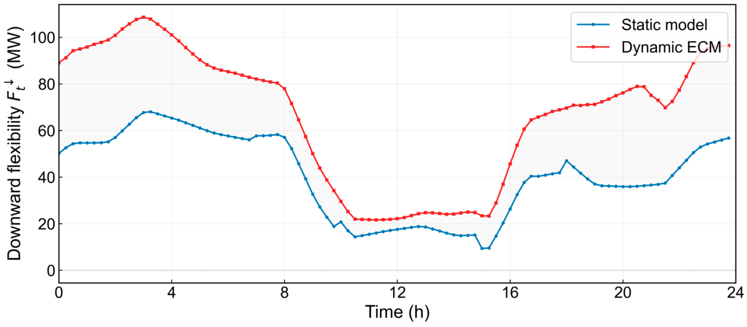
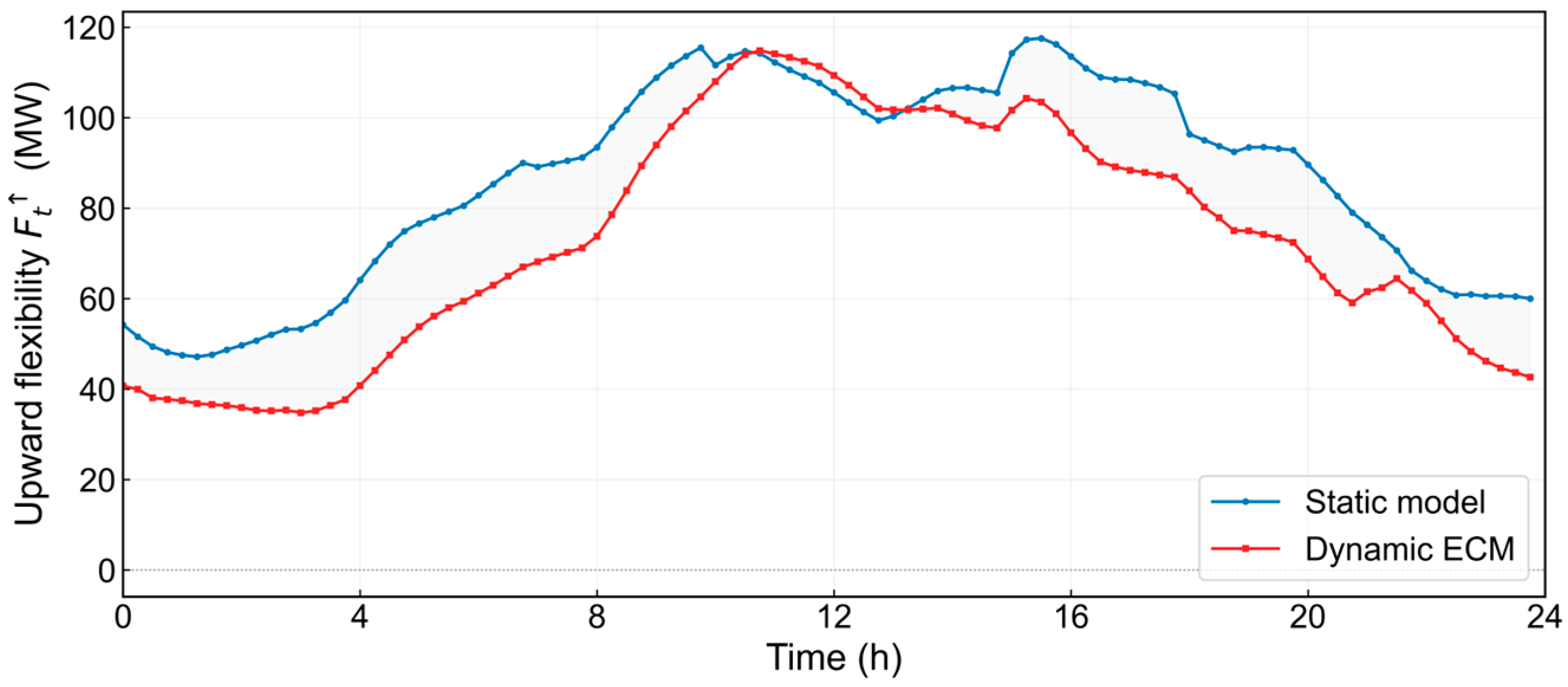
Despite this progress, existing dynamic multi-energy flexibility studies mainly quantify flexibility through system-level metrics, operational benefits, simulation-based profiles, or multidimensional admissible power-fluctuation regions. These representations are useful for revealing internal flexibility, but they are not directly aligned with grid-side regulation assessment, where the VPP is observed and scheduled through the net power exchanged at the PCC. Without an explicit projection onto this interface, the externally deliverable flexibility may be either overestimated, because internal thermal and gas constraints can prevent declared regulation from being delivered, or underestimated, because pipeline thermal storage and gas linepack may release additional regulation capability. Therefore, for an electricity–heating–gas VPP operated as a grid-facing entity, a key question remains: how can the joint time-varying feasible set formed by electric-network constraints, heating-network temperature dynamics, gas-network pressure dynamics, and multi-energy conversion devices be translated into period-wise PCC import and export limits? This mapping should also recover the feasible internal dispatch and state trajectories supporting each boundary point. Such a direct mapping from the joint dynamic feasible set to time-resolved PCC limits has not been sufficiently addressed by existing flexibility-assessment frameworks.

A further gap concerns the operational meaning of a calculated boundary. Heat transport delay, pipeline thermal storage, gas-pressure evolution, and linepack couple current PCC regulation to historical and terminal network states [18,19,20]. A schedule may therefore reach a large physical PCC extreme by depleting temperature or pressure margins near the end of the horizon, leaving the VPP unable to continue normal operation. Likewise, a physically attainable extreme may require an uneconomical combination of internal devices. Existing flexibility regions do not generally distinguish such short-term physical extremes from limits that are both state-sustainable and economically deployable. Consequently, the unresolved research gap is the lack of a PCC-oriented assessment framework that converts the joint dynamic feasibility of a multi-energy VPP into time-resolved external flexibility boundaries and screens the resulting extremes according to terminal-state and economic requirements.

The scientific problem addressed in this paper is therefore how to project the jointly coupled, time-varying feasible set of an electricity–heating–gas VPP onto the PCC net-power variable, while preserving historical temperature and pressure effects and distinguishing attainable limits from sustainable and economically deployable ones. To support repeated boundary optimization, the frequency-domain ECM is adopted to convert heating- and gas-network dynamics into algebraic constraints, retaining thermal propagation, gas-pressure evolution, and historical-state dependence without dense time–space discretization [21,22]. In this way, each calculated PCC boundary point is supported by a feasible internal state trajectory.

Accordingly, the main contributions of this paper are summarized as follows:

(1) An interface-oriented dynamic feasible-set projection framework is formulated for electricity–heating–gas VPPs. The proposed formulation directly optimizes the PCC net power over the jointly coupled dynamic feasible set, and obtains period-wise import and export limits together with the internal dispatch and state trajectories supporting each boundary point.

(2) A state-aware boundary formulation is established by embedding heating-network temperature dynamics, gas-network pressure dynamics, electric-network constraints, and multi-energy conversion devices into a unified boundary optimization. This formulation links historical network states and available temperature/pressure margins to coupling-device feasibility and ultimately to the time variation and directional asymmetry of the PCC flexibility boundary, providing a mechanism-based interpretation beyond the qualitative recognition of thermal inertia and gas linepack.

(3) A hierarchical characterization of physical, sustainable, and economically deployable flexibility is developed. Terminal-state recovery constraints prevent the boundary from being artificially enlarged through end-of-horizon depletion of pipeline storage, while an economic feasibility constraint excludes physically feasible but excessively costly schedules. This distinction provides a transferable principle for converting a technical multi-energy feasible range into grid-callable flexibility.

2. Dynamic ECM-Based Operation Model for the Electricity–Heating–Gas VPP

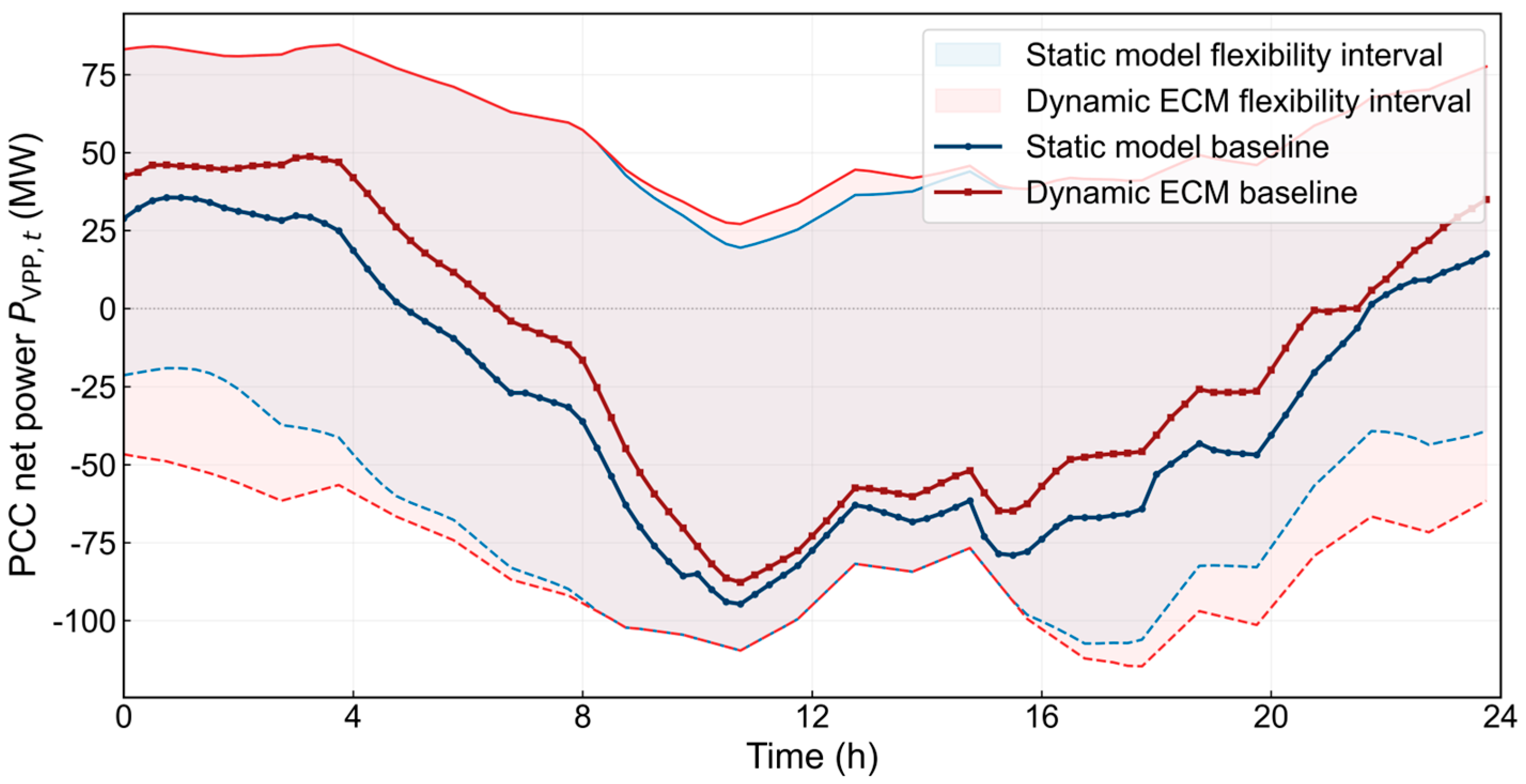
To evaluate the external flexibility of an electricity–heating–gas virtual power plant (VPP), the electric power flow, heating-network temperature dynamics, gas-network pressure dynamics, and multi-energy coupling-device constraints must be considered in a unified framework. Conventional static energy-flow models typically represent heating and gas networks using instantaneous steady-state balance equations, and therefore do not explicitly capture heat transmission delays, thermal inertia, or gas linepack effects [23]. To address this limitation, this section formulates a dynamic energy circuit model (ECM) to represent the operating states of the internal electric, heating, and gas subsystems under coupled dynamic network constraints.

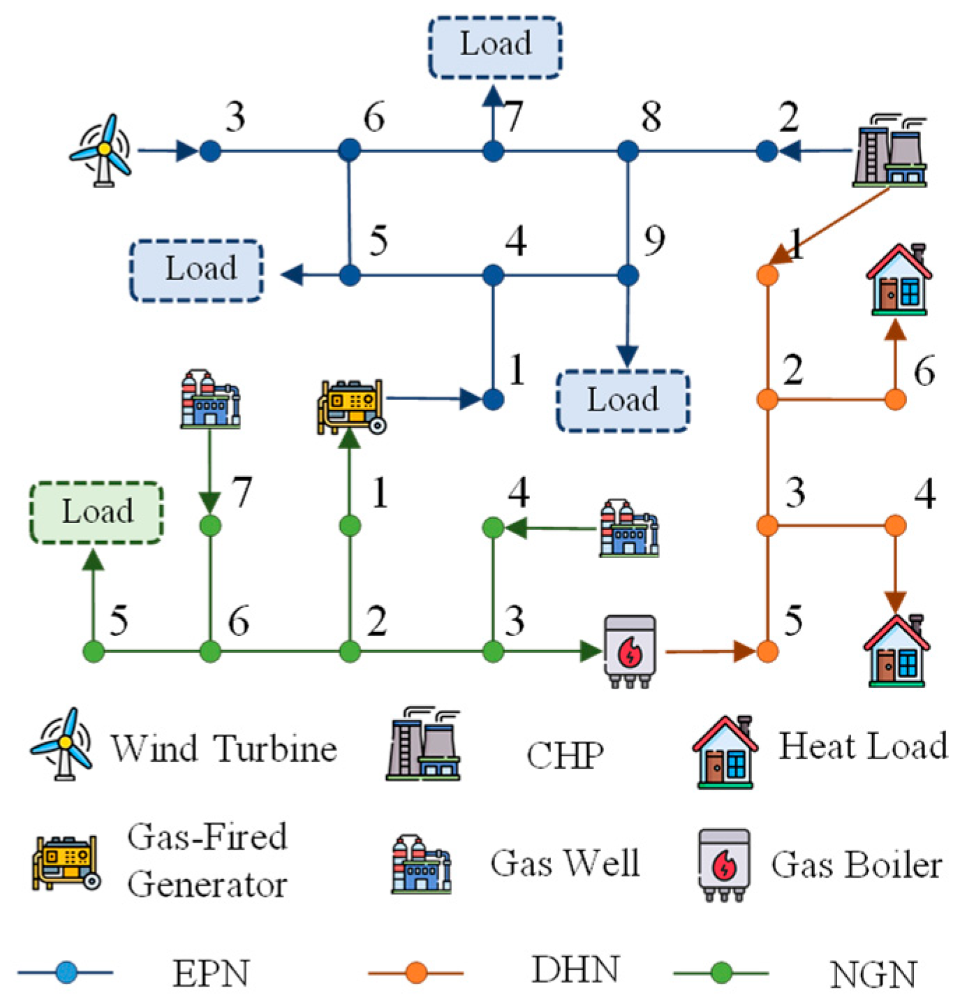
To make the modeling scope explicit, the principal assumptions and simplifications adopted in this study, together with their possible influence on the calculated flexibility boundaries, are summarized as follows. (1) The electric network uses lossless DC power flow, which may yield optimistic PCC boundaries. (2) Heating-pipe mass flows and directions are fixed, excluding variable-flow flexibility. (3) Gas dynamics are linearized around a nominal point and may be inaccurate under large deviations. (4) Load and wind-power forecasts are deterministic, so the boundaries are forecast-dependent.

2.1. Electric Power Network (EPN) Operation Model

At the VPP scheduling time scale, electromagnetic transients in the electric network are much faster than the dispatch interval. Therefore, the electric network is represented by a steady-state DC power-flow model. Let $p_{e,t}$ be the active-power net injection vector of electric nodes in period t, and let $f_{e,t}$ be the corresponding line-flow vector. Under the DC power-flow approximation, the line flows are given by

$$f_{e,t}=H_e{p}_{e,t},$$

(1)

where $H_e$ is the power transfer distribution factor matrix. The nodal active-power balance is enforced as

$$1^T{p}_{e,t}=0,$$

(2)

and the line security constraint is expressed as

$$-{\overline{f}}_e\le H_e{p}_{e,t}\le {\overline{f}}_e.$$

(3)

The nodal net injection is determined by the electric outputs of internal generation units, wind generation, electric loads, electric-to-heat devices, and the power exchanged at the point of common coupling (PCC). Thus, we have:

$$p_{e,t}=p_{e,t}^{\mathrm{gen}}+p_{e,t}^{\mathrm{wind}}-p_{e,t}^{\mathrm{load}}-p_{e,t}^{\mathrm{conv}}+p_{e,t}^{\mathrm{PCC}}.$$

(4)

Here, $p_{e,t}^{\mathrm{gen}}$ includes the electric outputs of conventional units, gas-fired units, and CHP units; $p_{e,t}^{\mathrm{wind}}$ represents wind power; $p_{e,t}^{\mathrm{load}}$ represents electric load; $p_{e,t}^{\mathrm{conv}}$ denotes the electric consumption of heat pumps, electric boilers, and other electric-to-heat devices; and $p_{e,t}^{\mathrm{PCC}}$ is the power exchanged with the external grid. The PCC exchange variable enters the nodal active-power balance at the designated interface bus. Under the adopted lossless DC power-flow approximation, active transmission losses within the VPP electric network are neglected.

Wind-power output is modeled as a bounded dispatch variable rather than a fixed injection. For each wind turbine w and period t, its scheduled output satisfies $0 \le {P^W}_{w,t}\le {P^{W,fore}}_{w,t}$, where ${P^{W,fore}}_{w,t}$ is the forecast available wind power. Thus, downward adjustment through wind curtailment is allowed, whereas wind power cannot be scheduled above its forecast availability.

2.2. District Heating Network (DHN) Operation Model

In a district heating network, thermal energy is transported by the working fluid. As a result, the network exhibits heat transmission delays and thermal inertia. A change in heat-source output cannot be instantaneously reflected at load nodes; instead, the temperature response depends on pipe length, flow velocity, heat loss, and historical temperature states. Therefore, heating-network dynamics should be explicitly retained in the flexibility boundary assessment.

The district heating network is assumed to operate in quality-regulation (temperature-regulation) mode. Accordingly, the mass-flow rate and nominal flow direction of each heating pipe are prescribed and remain unchanged throughout the scheduling horizon. For each heating pipe b, this condition is expressed as

$${\dot{m}}_{b,t}^H={\dot{m}}_b^{H,0}> 0$$

where ${\dot{m}}_b^{H,0}$ denotes the prescribed mass-flow rate of pipe b. The positive sign corresponds to its predefined from-node–to-node direction. Therefore, the flow velocity and the associated frequency-domain pipe parameters are fixed before the boundary optimization.

Under this assumption, the model retains temperature propagation delay, heat attenuation, pipeline thermal storage, and historical-state dependence for the prescribed hydraulic operating condition. Relative to a fully variable-flow formulation, fixing the mass-flow rates and directions removes hydraulic control degrees of freedom and may therefore produce a conservative estimate of the total flexibility range. If the actual mass flow differs appreciably from the prescribed value, however, both heat-transport delay and attenuation change, and the resulting temperature constraints may shift either the upper or lower PCC boundary. Thus, the direction of the boundary error cannot be stated universally. The present model is mainly applicable to district heating systems with stable mass-flow settings and no flow reversal over the scheduling horizon.

For a heating branch $l=(i,j)$, let $T_l(x,t)$ be the working-fluid temperature at position $x$ and time $t$, $v_l$ denote the flow velocity, $T_a$ denote the ambient temperature, and ${\kappa }_l$ denote the heat-loss coefficient. The temperature dynamics along the pipe are described by:

$${\displaystyle \frac{\partial T_l(x,t)}{\partial t}}+v_l{\displaystyle \frac{\partial T_l(x,t)}{\partial x}}=-{\kappa }_l[T_l(x,t)-T_a],$$

(5)

which indicates that the outlet temperature is governed not only by the current inlet temperature but also by historical inlet temperatures and the pipe heat-transfer process. In the frequency-domain ECM, this dynamic inlet–outlet relationship can be transformed into an algebraic form. For the $k$-th frequency component, the branch temperature relation is given by:

$${\widehat{T}}_{j,k}=G_{ij,k}^h{\widehat{T}}_{i,k}+{\widehat{s}}_{ij,k}^h,$$

(6)

where $G_{ij,k}^h$ is the transfer coefficient of heating branch $(i,j)$, and ${\widehat{s}}_{ij,k}^h$ is the equivalent term associated with ambient temperature, boundary conditions, and historical states. By assembling all branch-level relations according to the heating-network topology, the network-level frequency-domain model can be written as:

$${\widehat{\theta }}_{h,k}=Z_{h,k}\cdot {\widehat{q}}_{h,k}+{\widehat{r}}_{h,k}^{his}$$

(7)

The frequency-domain model is then transformed back to the time domain, yielding

$${\theta }_h={\mathcal{M}}_h{q}_h+r_h^{\mathrm{his}}$$

(8)

where

$${\mathcal{M}}_h={\mathcal{F}}^{-1}\mathrm{blkdiag}(Z_{h,0},Z_{h,1},\dots ,Z_{h,K-1})\mathcal{F}.$$

(9)

Here, $\mathcal{F}$ is the discrete Fourier transform matrix. The vector $q_h$ is the heat-power injection sequence over the optimization window, ${\theta }_h$ is the heating-network temperature-state sequence, and $r_h^{\mathrm{his}}$ is the equivalent influence of historical temperatures and heat injections mapped into the target scheduling interval through the frequency-domain ECM. The temperature security limits of the heating network are imposed as

$$\underset{¯}{{\theta }_h}\le {\mathcal{M}}_h{q}_h+r_h^{\mathrm{his}}\le \overline{{\theta }_h},$$

(10)

which embeds the effect of heating-network dynamics into the VPP flexibility assessment. Pipe heat storage can support short-term electric-power regulation, while temperature limits and transmission delays restrict the adjustable ranges of CHP units, heat pumps, and gas boilers.

2.3. Natural Gas Network (NGN) Operation Model

Natural gas networks exhibit appreciable dynamic characteristics because gas compressibility enables pipelines to store gas through linepack effects. Variations in the gas consumption of gas-fired generators and gas boilers directly affect nodal pressures, while the pressure evolution is constrained by historical operating states and available linepack capacity. Therefore, gas-network dynamics influence the capability of gas-fired devices to provide flexibility regulation for the VPP.

For a natural gas pipe $l=(i,j)$, let ${\pi }_l(x,t)$ denote the pressure variable and $m_l(x,t)$ the mass flow. The linearized dynamic equations of the gas pipeline are expressed as

$${\displaystyle \frac{\partial {\pi }_l(x,t)}{\partial t}}+a_l{\displaystyle \frac{\partial m_l(x,t)}{\partial x}}=0,$$

(11)

$${\displaystyle \frac{\partial m_l(x,t)}{\partial t}}+b_l{\displaystyle \frac{\partial {\pi }_l(x,t)}{\partial x}}+c_l{m}_l(x,t)=0.$$

(12)

The coefficients $a_l$,$b_l$,$c_l$ are determined by pipe parameters and the operating base point. These linearized relations retain the dominant gas-network dynamics around the nominal operating point while avoiding nonlinear coupling in the repeated boundary optimization. The detailed derivation, linearization treatment, and approximation-error validation of the adopted ECM are provided in [21,22]. Through frequency-domain transformation, the dynamic gas-network equations are converted into algebraic forms. For the k_th frequency component, the network-level pressure relation is given by:

$${\widehat{\pi }}_{g,k}=Z_{g,k}{\widehat{m}}_{g,k}+{\widehat{r}}_{g,k}^{\mathrm{his}},$$

(13)

where ${\widehat{m}}_{g,k}$ is the frequency component of nodal gas net injection, $Z_{g,k}$ is the frequency-domain impedance matrix of the gas network, and ${\widehat{r}}_{g,k}^{\mathrm{his}}$ represents the equivalent influence of historical pressures and gas injections mapped by the frequency-domain ECM. Transforming the frequency-domain model back to the time domain gives

$${\pi }_g={\mathcal{M}}_g{m}_g+r_g^{\mathrm{his}}$$

(14)

$${\mathcal{M}}_g={\mathcal{F}}^{-1}\mathrm{blkdiag}(Z_{g,0},Z_{g,1},\cdots ,Z_{g,K-1})\mathcal{F}.$$

(15)

Here, $m_g$ is the gas net-injection sequence over the optimization window, ${\pi }_g$ is the gas-node pressure sequence, and $r_g^{\mathrm{his}}$ represents the contribution of historical line pack and initial pressure states to the current scheduling window. The pressure safety constraint of the gas network is imposed as

$$\underset{¯}{{\pi }_g}\le {\mathcal{M}}_g{m}_g+r_g^{\mathrm{his}}\le \overline{{\pi }_g},$$

(16)

This constraint reflects the impact of gas line pack and pressure dynamics on the flexibility boundary. When sufficient pressure margin is available, line pack can temporarily support the regulation of gas-fired devices. Conversely, when nodal pressures approach their limits, the adjustable capability of gas-consuming devices is restricted.

2.4. Multi-Energy Coupling Device Model

The VPP considered in this paper includes natural gas units, CHP units, gas boilers, heat pumps, and other multi-energy coupling devices. Their variables are connected to the electric, heating, and gas networks through nodal injection terms, and thus affect the PCC net power and the resulting flexibility boundary.

2.4.1. Energy Conversion Models

A natural gas unit (NGU) converts gas into electric power. The gas consumption and electric output of NGU $i$ in period $t$ satisfy:

$$m_{i,t}^{\mathrm{NGU}}=r_i^{\mathrm{NGU}}{P}_{i,t}^{\mathrm{NGU}},$$

(17)

where $P_{i,t}^{\mathrm{NGU}}$ is the electric output, $m_{i,t}^{\mathrm{NGU}}$ is its gas consumption, and $r_i^{\mathrm{NGU}}$ is the gas-to-electric conversion coefficient.

A CHP unit produces electric and thermal power simultaneously. Under a fixed heat-to-electric ratio, its output relation is expressed as:

$$h_{i,t}^{\mathrm{CHP}}=r_i^{\mathrm{CHP}}{P}_{i,t}^{\mathrm{CHP}},$$

(18)

where $P_{i,t}^{\mathrm{CHP}}$ and $h_{i,t}^{\mathrm{CHP}}$ denote the electric and heat output, respectively, and $r_i^{\mathrm{CHP}}$ is the heat-to-electric ratio.

A gas boiler converts gas into heat. The corresponding conversion relation is:

$$m_{i,t}^{\mathrm{GB}}=r_i^{\mathrm{GB}}{h}_{i,t}^{\mathrm{GB}}.$$

(19)

Here $h_{i,t}^{\mathrm{GB}}$ is the heat output, $m_{i,t}^{\mathrm{GB}}$ is the gas consumption, and $r_i^{\mathrm{GB}}$ is the gas-to-heat conversion coefficient.

A heat pump consumes electric power and supplies heat to the heating network. Its electric consumption and heat output are related by

$$P_{i,t}^{\mathrm{HP}}=r_i^{\mathrm{HP}}{h}_{i,t}^{\mathrm{HP}},$$

(20)

where $P_{i,t}^{\mathrm{HP}}$ is the electric consumption of the heat pump, $h_{i,t}^{\mathrm{HP}}$ is its heat output, and $r_i^{\mathrm{HP}}$ is the coefficient of performance.

2.4.2. Device Operating Constraints

For a controllable device $u$, let $x_{u,t}$ denote its operating variable in period $t$. The output limits are uniformly expressed as

$$x_u^{\min }\le x_{u,t}\le x_u^{\max },$$

(21)

and the ramping constraint is given by

$$-R_u^{\downarrow }\le x_{u,t}-x_{u,t-1}\le R_u^{\uparrow }.$$

(22)

Here, $x_{u,t}$ can represent the electric output of a gas-fired unit, the electric output of a CHP unit, the heat output of a gas boiler, the heat output of a heat pump, or the gas supply of a gas source.

2.4.3. Nodal Injections of Coupling Devices

Multi-energy coupling devices enter the electric, heating, and natural gas-network models through nodal injection terms. Let $j\in i$ denote that device $j$ is connected to node $i$. The electric net injection at node $i$ in period $t$ is formulated as

$$P_{n,i,t}={\displaystyle \sum }_{j\in i}{P}_{\mathrm{tpu},j,t}+{\displaystyle \sum }_{j\in i}{P}_{\mathrm{ngu},j,t}+{\displaystyle \sum }_{j\in i}{P}_{\mathrm{chp},j,t}+{\displaystyle \sum }_{j\in i}{P}_{\mathrm{wt},j,t}-{\displaystyle \sum }_{j\in i}{P}_{\mathrm{hp},j,t}-P_{\mathrm{ld},i,t}.$$

(23)

The first four terms represent the electric outputs of conventional thermal units, gas-fired units, CHP units, and wind turbines, respectively. The fifth term is the electric consumption of heat pumps, and the last term is the electric load. Thus, gas-fired units, CHP units, and wind turbines act as positive injections in the electric network, whereas heat pumps and electric loads act as negative injections.

The gas net injection at node $i$ is

$$m_{n,i,t}={\displaystyle \sum }_{j\in i}{m}_{\mathrm{gw},j,t}-{\displaystyle \sum }_{j\in i}{m}_{\mathrm{ngu},j,t}-{\displaystyle \sum }_{j\in i}{m}_{\mathrm{gb},j,t}-m_{\mathrm{ld},i,t},$$

(24)

where gas sources are positive injections, while gas-fired units, gas boilers, and gas loads are negative injections.

Similarly, the heat-power net injection at a heating node or pipe inlet is given by

$$h_{n,i,t}={\displaystyle \sum }_{j\in i}{h}_{\mathrm{chp},j,t}+{\displaystyle \sum }_{j\in i}{h}_{\mathrm{gb},j,t}+{\displaystyle \sum }_{j\in i}{h}_{\mathrm{hp},j,t}-h_{\mathrm{ld},i,t}.$$

(25)

CHP units, gas boilers, and heat pumps act as heat sources, while heat loads are negative injections. Through these nodal injection relationships, different heat-source combinations can satisfy heat demand while simultaneously affecting the electric and natural gas-network states.

2.5. Time–Frequency Consistency Constraints for Coupling-Device Injections

Since the heating- and gas-network constraints are formulated in the frequency domain, the gas-side and heat-side injection variables of coupling devices must be consistent with their corresponding time-domain operating variables. Therefore, in addition to the time-domain output limits, ramping limits, and energy-conversion constraints, a discrete Fourier transform (DFT) relationship is imposed between the time-domain device sequences and the frequency-domain network injection variables.

Taking the gas consumption of NGU $i$ as an example, its time-domain sequence over the optimization horizon is

$${\left\{m_{\mathrm{ngu},i,t}\right\}}_{t=1}^T.$$

(26)

The corresponding $k$-th frequency-domain component is obtained by

$$m_{\mathrm{ngu},i}^{(k)}={\displaystyle {\displaystyle \sum }_{t=1}^T}{\mathsf{\Gamma }}_{k,t}{m}_{\mathrm{ngu},i,t}.$$

(27)

Here, ${\mathsf{\Gamma }}_{k,t}$ are the elements of the discrete Fourier transform matrix. The same mapping is applied to gas-boiler consumption, gas-source supply, and heat-power injection variables. Through these time–frequency consistency constraints, multi-energy coupling devices are linked to the frequency-domain heating and gas-network models via nodal injections, thereby affecting the electric-, heating-, and gas-network states as well as the PCC net power.

3. Operational Flexibility Boundary Assessment Model

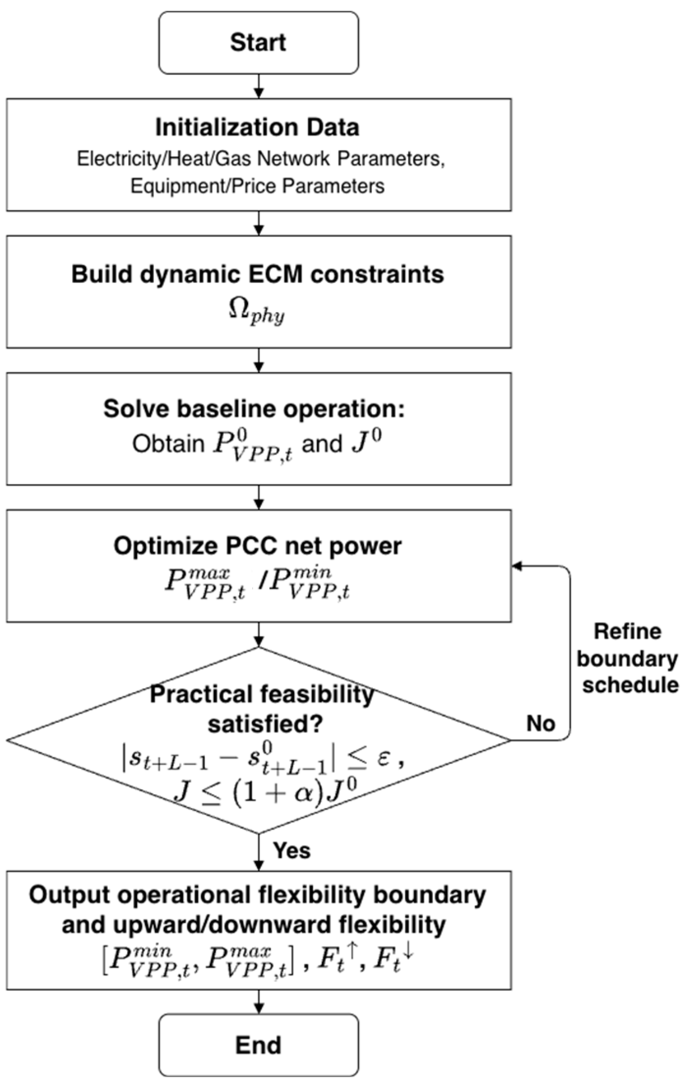
Based on the dynamic ECM-based operation model established in Section 2, this section formulates an optimization-based operational flexibility boundary assessment model. The PCC net power is selected as the external flexibility interface, while the electric, heating, gas, and coupling-device constraints define the internal feasible operating set of the VPP. By maximizing and minimizing the PCC net power over this feasible set, the physical upper and lower flexibility boundaries are obtained for each scheduling period. Upward and downward flexibility indices are then defined relative to the baseline operating point. Terminal recovery and economic feasibility constraints are further introduced to prevent excessive use of network storage and to ensure that the boundary schedules remain practically acceptable.

3.1. PCC Net Power of the VPP

With the PCC net power selected as the external interface variable, $P_{\mathrm{vpp},t}$ is defined as the net active power exchanged between the VPP and the external grid in period $t$. A positive value of $P_{\mathrm{vpp},t}$ indicates power export from the VPP to the external grid, whereas a negative value indicates power import from the external grid.

According to the active-power balance of the internal electric subsystem, $P_{\mathrm{vpp},t}$ can be expressed as:

$$P_{\mathrm{VPP},t}={\displaystyle \sum }_i{P}_{i,t}^{\mathrm{TPU}}+{\displaystyle \sum }_i{P}_{i,t}^{\mathrm{NGU}}+{\displaystyle \sum }_i{P}_{i,t}^{\mathrm{CHP}}+{\displaystyle \sum }_i{P}_{i,t}^{\mathrm{WT}}-{\displaystyle \sum }_i{P}_{i,t}^{\mathrm{HP}}-{\displaystyle \sum }_i{P}_{i,t}^{\mathrm{load}}.$$

(28)

The positive terms represent electric power supplied by conventional thermal units, natural gas units, CHP units, and wind turbines, while the negative terms represent heat-pump electricity consumption and electric load. Thus, $P_{\mathrm{vpp},t}$ provides a compact external representation of the internal electric dispatch of the VPP. For economic evaluation, the PCC net power is further decomposed into selling and buying variables:

$$P_{\mathrm{VPP},t}=P_{\mathrm{export},t}-P_{\mathrm{import},t}.$$

(29)

Here, $P_{\mathrm{export},t}$ and $P_{\mathrm{import},t}$ denote the power sold to and purchased from the external grid, respectively. The corresponding electricity prices satisfy

$$0\le {\pi }_{\mathrm{sell},t}\le {\pi }_{\mathrm{buy},t},$$

(30)

where ${\pi }_{\mathrm{buy},t}$ and ${\pi }_{\mathrm{sell},t}$ are the buying and selling prices, respectively. This relationship is used in the economic feasibility constraint introduced later.

3.2. Physical Operational Flexibility Boundary

Based on the dynamic ECM-based operation model in Section 2 and the PCC net-power definition in Section 3.1, the physical feasible operation set of the VPP is denoted by ${\mathsf{\Omega }}_{\mathrm{phy}}$. This set includes the steady-state electric power-flow constraints, district-heating temperature dynamic constraints, natural gas pressure dynamic constraints, multi-energy coupling-device constraints, time-frequency consistency constraints, device output and ramping limits, and network security limits. For compactness, it is written as:

$${\mathsf{\Omega }}_{\mathrm{phy}}=\{\mathbf{x},\mathbf{u}|all operational constraints \mathrm{are} \mathrm{satisfied}\}$$

(31)

Under ${\Omega }_{\mathrm{phy}}$, the upper operational flexibility boundary of the VPP in period $t$ is defined as

$$P_{\mathrm{VPP},t}^{\max }=\underset{\mathbf{x},\mathbf{u}}{\max }{P}_{\mathrm{VPP},t}$$

(32)

$$\mathrm{s}.\mathrm{t}. (x,u)\in {\Omega }_{\mathrm{phy}},$$

(33)

and the lower boundary is defined as

$$P_{\mathrm{VPP},t}^{\min }=\underset{\mathbf{x},\mathbf{u}}{\min }{P}_{\mathrm{VPP},t}$$

(34)

$$\mathrm{s}.\mathrm{t}. (x,u)\in {\Omega }_{\mathrm{phy}}.$$

(35)

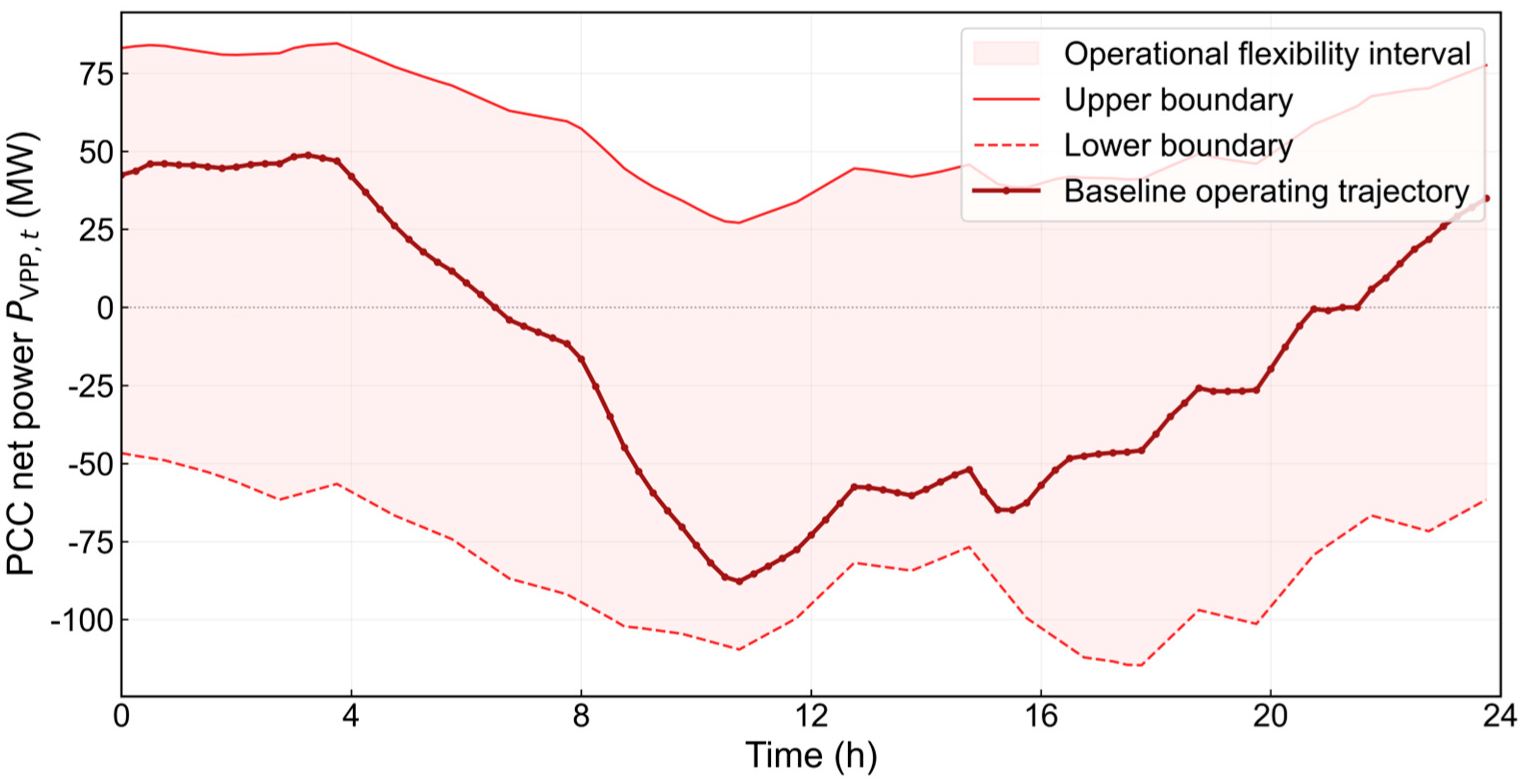
Therefore, the physical operation flexibility interval in period $t$ is

$$P_{\mathrm{VPP},t}^{\min }\le P_{\mathrm{VPP},t}\le P_{\mathrm{VPP},t}^{\max }.$$

(36)

This interval represents the reachable range of PCC net power without violating the internal electric, heating, gas, and device operating constraints. It is not obtained by a simple summation of individual device capacities; rather, it is the projection of the coupled dynamic feasible region of the electricity–heating–gas VPP onto the external net-power interface.

3.3. Upward and Downward Flexibility Indices

The baseline operating point represents the normal dispatch schedule of the VPP under forecasted load, renewable generation, and price conditions. Let $P_{\mathrm{vpp},0}$ denote the PCC net power at this baseline operating point in period $t$. For a specified PCC flexibility boundary $[P_{\mathrm{VPP},t}^{\min },P_{\mathrm{VPP},t}^{\max }]$, the upward flexibility of the VPP relative to the baseline trajectory is defined as

$$F_t^{\uparrow }=P_{\mathrm{VPP},t}^{\max }-P_{\mathrm{VPP},t}^0,$$

(37)

and the downward flexibility is

$$F_t^{\downarrow }=P_{\mathrm{VPP},t}^0-P_{\mathrm{VPP},t}^{\min }.$$

(38)

Here, $F_t^{\uparrow }$ and $F_t^{\downarrow }$ characterize the upward and downward flexibility margins relative to the baseline operating point, respectively. The upward margin corresponds to the additional PCC net power that can be provided through generation increase, load reduction, or reduced electric-to-heat consumption. The downward margin corresponds to the reducible PCC net power, or additional import capability, enabled by generation reduction, increased heat-pump consumption, or coordinated adjustment of multi-energy coupling devices.

The absolute PCC boundaries and the baseline-referenced flexibility margins have different roles. The extrema defined in Section 3.2 represent the scenario-conditioned reachable export and import limits and are independent of a scheduled PCC value. Their differences from the committed day-ahead baseline quantify the remaining upward and downward adjustment capability and are suitable for reserve-capacity and ancillary-service assessment. Changing the baseline therefore reallocates the upward and downward margins but does not alter the underlying PCC boundary under the same feasible set.

The baseline trajectory is obtained first through a full-horizon economic dispatch under the same dynamic-network, device, security, historical-state, forecast, price, and capacity conditions used in the boundary calculation. This baseline optimization provides the reference PCC trajectory, the baseline operating cost, and the corresponding terminal network states. The terminal states and operating cost obtained from this baseline solution are subsequently used as references in the terminal-recovery and economic-feasibility constraints introduced in Section 3.4.

Other flexibility representations include ramping flexibility, cumulative energy flexibility, joint multi-period trajectory regions, and cost–flexibility curves. This study reports the period-wise PCC envelope and its baseline-referenced upward and downward margins because grid regulation is scheduled around a committed PCC trajectory.

3.4. Terminal Recovery and Economic Feasibility Constraints

The physical flexibility boundary defined in Section 3.2 characterizes the maximum reachable PCC net-power range under the dynamic network and device operating constraints. However, a physically reachable boundary schedule may not be practically sustainable if it excessively exploits heating-network thermal storage or gas-network linepack, and it may also be economically unattractive if it relies on high-cost internal dispatch. Therefore, the proposed framework distinguishes three nested levels of flexibility: the physical boundary, the sustainable boundary obtained by additionally imposing terminal-state recovery, and the economically deployable boundary obtained by further imposing the economic-feasibility constraint.

To obtain the sustainable boundary, the terminal state of each boundary schedule is constrained to remain sufficiently close to the terminal state of the baseline economic dispatch. Let $s_{t+L-1}$ denote the key state variables at the end of the window, including heating-network temperatures, gas-network pressures, and device outputs. Let $s_{t+L-1}^0$ denote the corresponding baseline states. The terminal recovery constraint is expressed as:

$$\mid s_{t+L-1}-s_{t+L-1}^0\mid \le \epsilon ,$$

(39)

where $\epsilon$ is the allowed terminal-state deviation. This constraint limits excessive depletion or accumulation of pipeline thermal storage and gas-network linepack and prevents the calculated boundary from relying on an unfavorable end-of-horizon state. The resulting boundary is therefore referred to as the sustainable flexibility boundary.

To further obtain an economically deployable boundary, an economic-feasibility constraint is imposed on the sustainable boundary schedules to exclude operating strategies that require excessive additional cost solely to enlarge the PCC regulation range. Let $J$ denote the total operating cost of a boundary schedule over the scheduling horizon, including conventional-unit cost, gas-fired-unit cost, gas-boiler cost, PCC transaction cost, and penalty cost. It is expressed as:

$$J={\displaystyle \sum _{t\in W}\left(C_t^{\mathrm{TPU}}+C_t^{\mathrm{NGU}}+C_t^{\mathrm{GB}}+C_t^{\mathrm{PCC}}+C_t^{\mathrm{pen}}\right)},$$

(40)

where the PCC transaction cost is

$$C_t^{\mathrm{PCC}}={\pi }_{\mathrm{buy},t}{P}_{\mathrm{import},t}-{\pi }_{\mathrm{sell},t}{P}_{\mathrm{export},t}.$$

(41)

Let $J^0$ be the baseline dispatch cost and $\alpha$ the allowed cost-deviation ratio. The economic feasibility constraint is then given by

$$J\le (1+\alpha )J^0.$$

(42)

This constraint ensures that the internal dispatch supporting each retained boundary point remains economically acceptable relative to normal operation. Consequently, the three flexibility levels satisfy a nested relationship: the sustainable boundary is contained within the physical boundary, and the economically deployable boundary is further contained within the sustainable boundary.

4. Solution Procedure

The solution procedure for the proposed operational flexibility boundary assessment model is shown in Figure 1. First, the electric-, heating-, and gas-network parameters, device parameters, load and wind forecasts, historical boundary conditions, and price parameters are initialized. Second, the dynamic ECM-based operation constraints are constructed, including the steady-state electric power-flow constraints, heating-network temperature dynamic constraints, gas-network pressure dynamic constraints, and multi-energy coupling-device constraints. Third, the baseline economic-dispatch problem is solved to obtain the reference PCC trajectory $P_{\mathrm{vpp},0}$ and baseline operating cost $J^0$. Fourth, the physical upper and lower PCC boundaries are obtained by maximizing and minimizing the PCC net power under the dynamic operation constraints. The terminal-recovery constraint is then imposed to obtain the sustainable boundary, after which the economic-feasibility constraint is further imposed to obtain the economically deployable boundary. Finally, the upward and downward flexibility margins are evaluated relative to the baseline PCC trajectory. The upward and downward flexibility indices are then obtained based on the accepted boundary results. The proposed formulation is not restricted to a specific VPP topology and can be extended by updating the network matrices, device parameters, and coupling relationships. For larger systems, the computational burden increases with the network size, scheduling horizon, and number of retained frequency components, while sparse computation and parallel solution of period-wise boundary problems provide potential acceleration strategies. Comprehensive validation on large-scale VPPs is left for future work.

5. Case Study

5.1. Basic Data

The proposed method is evaluated on the P9H12G7 electricity–heating–gas VPP test system originally reported in [21]. Its network topology, equipment composition, and network and device physical parameters are adopted directly from [21] without modification. The system comprises a 9-bus EPN, a 12-node DHN, and a 7-node NGN, as shown in Figure 2. In the P9H12G7 system, electric bus 8 is designated as the PCC reference bus and represents the interface with the upstream grid. The test system includes three energy infrastructures, multi-energy conversion units, renewable generation, and heterogeneous energy demands, including electric lines, heating pipelines, gas pipelines, conventional generators, CHP units, wind turbines, gas-fired units, gas boilers, electric loads, heating loads, and gas loads. Reference [21] used this system to demonstrate a frequency-domain optimal energy flow formulation, whereas the present study uses the unchanged system to assess the PCC-oriented operational flexibility boundary. Readers are referred to [21] for the complete topology and physical dataset. The scheduling horizon consists of 96 time intervals with a 15 min resolution, representing a one-day operational horizon. This resolution is consistent with typical day-ahead and intra-day scheduling practices and provides a balance between capturing the intertemporal coupling caused by heating-network thermal inertia and gas-network linepack effects and maintaining computational tractability. A one-day horizon is adopted to ensure that the historical-state dependence and terminal-state recovery requirements of dynamic energy networks are properly considered during flexibility-boundary assessment. A coarser temporal resolution may smooth short-term dynamic or ramping constraints and thereby overestimate the available flexibility in some periods, whereas a shorter scheduling horizon may insufficiently capture state recovery and intertemporal energy shifting. A baseline operating point is first obtained by solving the economic dispatch problem, where the objective considers internal device operating costs and PCC electricity transaction costs. The quotation parameters of conventional generating units are adopted from [24].

Deterministic day-ahead wind-power forecasts are adopted in the present case study and are assumed to be perfectly realized during the flexibility-boundary calculation. Wind curtailment is allowed through the bounded wind-power dispatch described in Section 2.1. Accordingly, the reported PCC flexibility boundaries are conditional on the adopted forecast trajectory; no stochastic scenarios, robust uncertainty set, or explicit reserve for wind-power forecast errors is included.

The validation was conducted at the application level to examine the operational consistency and practical applicability of the dynamic ECM-based flexibility assessment. First, a baseline economic dispatch was obtained under the forecast load, wind-power availability, device constraints, and dynamic network constraints. Second, the PCC net power was separately maximized and minimized in each period to obtain the upper and lower boundaries. Only boundary schedules satisfying the electric-network constraints, heating-network temperature dynamics, gas-network pressure dynamics, time-frequency consistency constraints, device limits, and terminal-state recovery requirements were retained. The baseline PCC trajectory was then checked against the calculated flexibility envelope. Third, the dynamic ECM was compared with the static model under identical load profiles, wind-power availability, network topology, and device parameters, with the representation of heating- and gas-network dynamics being the only modeling difference. Finally, the total operating costs of the upper- and lower-boundary schedules were used to evaluate the economic feasibility of the resulting boundaries.

Compared with the static formulation, the dynamic ECM introduces additional cross-period heating- and gas-network constraints and therefore increases the computational burden. Nevertheless, it remained computationally tractable for the studied P9H12G7 system, with all boundary optimization problems solved to optimality. The computational burden mainly depends on the network size, scheduling horizon, and number of retained frequency components.

5.2. Simulation Result Analysis

Two modeling approaches are compared: the proposed dynamic ECM and a conventional static multi-energy model. The dynamic ECM explicitly captures the temperature propagation dynamics of the district heating network and the pressure evolution characteristics of the natural gas network. In contrast, the static model represents the heating and gas networks using steady-state balance equations, neglecting heat transmission delays, thermal storage effects in pipelines, and gas linepack dynamics. Both models are evaluated under identical load profiles, wind power availability, and device parameters, with the only difference being the representation of heating- and gas-network dynamics.

5.2.1. Operational Flexibility Boundary Obtained by the Dynamic ECM

Figure 3 illustrates the operational flexibility boundary obtained using the proposed dynamic ECM together with the baseline operating trajectory. The reported boundary schedules satisfy the terminal-state recovery requirement, thereby avoiding excessive end-of-horizon depletion of network storage.

The flexibility boundary exhibits significant temporal variations, demonstrating that the VPP flexibility cannot be characterized by simply aggregating the adjustment capacities of individual devices. Instead, it is jointly determined by the coupled operational constraints of the electric, heating, and natural gas networks, as well as the available flexibility of multi-energy conversion devices. When the baseline operating point approaches the upper boundary, the remaining capability to increase PCC net power becomes limited. Conversely, proximity to the lower boundary indicates reduced capability to further decrease net power exchange or absorb additional electrical power from the external grid.

5.2.2. Comparison of Flexibility Boundaries Between Dynamic and Static Models

Figure 4 compares the operational flexibility boundaries obtained from the static model and the proposed dynamic ECM. Both models exhibit similar temporal variations, indicating that the overall flexibility pattern is primarily determined by the underlying load profile, renewable generation availability, and device operating conditions. However, noticeable deviations appear between the two models, particularly in the lower-bound region.

The dynamic ECM produces a wider flexibility envelope in several periods because it captures the inter-temporal regulation capability provided by heating-network thermal storage and natural gas pipeline linepack. These dynamic effects allow part of the electrical regulation demand to be shifted and accommodated by other energy carriers, which is not captured by the static model. Therefore, neglecting network dynamics may lead to inaccurate estimation of the VPP flexibility boundary, especially for downward flexibility assessment.

5.2.3. Comparison of Upward and Downward Flexibility Between Dynamic and Static Models

Figure 5 compares the downward flexibility obtained by the static model and the dynamic ECM. The dynamic ECM consistently provides larger downward flexibility over the scheduling horizon, with more significant improvements occurring during periods when the heating and gas networks possess greater dynamic regulation capability. This enhancement originates from the storage characteristics embedded in multi-energy networks. Specifically, pipe thermal storage and gas linepack effects allow temporary energy imbalances to be accommodated across multiple time periods, thereby creating additional capacity for electric-power absorption at the PCC.

When downward regulation is required, the VPP can increase the consumption of electric-to-heat devices, modify the combination of heat supply units, or adjust gas-fired devices through the flexibility provided by the gas network. Consequently, part of the electrical regulation requirement can be transferred to the heating and gas subsystems. In contrast, the static model neglects these inter-temporal storage and transmission effects and therefore cannot capture the additional absorption capability provided by dynamic energy networks.

Figure 6 compares the upward flexibility under the two modeling approaches. Unlike downward flexibility, the improvement in upward flexibility is not consistent across all periods. The dynamic ECM produces comparable or slightly lower upward flexibility than the static model in several periods. This difference results from the additional temporal constraints introduced by dynamic energy networks. Increasing PCC net power requires higher electrical generation output, reduced electric-to-heat consumption, or coordinated adjustment of CHP operation, while simultaneously satisfying gas supply limitations, heating demand requirements, device output constraints, and terminal state recovery conditions.

By explicitly modeling these cross-period interactions, the dynamic ECM avoids the optimistic estimation of upward flexibility caused by static approximations. Therefore, the role of dynamic network characteristics is not simply to enlarge the flexibility boundary, but to provide a dynamically consistent characterization of the practically available flexibility. In particular, heating- and gas-network dynamics mainly enhance absorption-oriented flexibility, while upward flexibility remains primarily determined by generation capability, gas availability, and heat-demand constraints.

A representative-period sensitivity analysis was further conducted to examine the influence of heating-network thermal inertia and gas-pressure operating margins. Variations in thermal inertia mainly affected the lower PCC boundary and exhibited time-dependent, non-monotonic effects, indicating that thermal dynamics redistribute rather than uniformly enlarge the available flexibility. In contrast, ±10% variations in the admissible gas-pressure margin produced negligible boundary changes in the selected periods, indicating that the pressure-margin constraint was not limiting under these operating conditions.

5.2.4. Impact of Economic Constraints on the Flexibility Boundary

Table 1. Cost comparison before and after introducing the economic constraint.

Boundary Schedule	Without Economic Constraint (CNY)	With Economic Constraint (CNY)	Cost Reduction (%)
Upper-bound cost	339,773.33	242,455.07	28.64
Lower-bound cost	305,627.80	242,455.68	20.67

compares the operating costs of boundary schedules obtained with and without the economic constraint under the dynamic ECM. Without the economic constraint, the boundary optimization may retain operationally sustainable but economically inefficient dispatch schemes that rely excessively on costly internal resources. Therefore, the economic constraint further refines the sustainable boundary into an economically deployable flexibility range.

Using the total operating cost over the 96-period horizon as the economic metric, the economic constraint reduces the upper- and lower-boundary scheduling costs by 28.64% and 20.67%, respectively. These results indicate that the economic constraint effectively excludes boundary schedules that rely excessively on high-cost internal resources. The retained boundary points continue to satisfy the dynamic network and device constraints, but are achieved using more economically acceptable internal dispatch combinations. Therefore, the resulting flexibility range represents economically deployable capability rather than an unconstrained physical extreme.

Overall, the dynamic unified ECM provides a dynamically consistent characterization of the operational flexibility boundary of the electricity–heating–gas VPP by capturing the temporal coupling of multi-energy networks. Compared with the static model, the dynamic ECM reveals additional downward flexibility enabled by pipe thermal storage and gas linepack effects, while correcting the inaccurate estimation of flexibility caused by neglecting dynamic network behaviors. The economic constraint further improves the practical applicability of the boundary schedules by ensuring their cost effectiveness.

Wind-power forecast errors would change the available-generation constraint and thereby alter the feasible set projected onto the PCC. A negative forecast error would primarily reduce the upper power-export boundary and could render a previously calculated upper-boundary schedule infeasible if other internal resources cannot compensate for the shortfall. A positive forecast error could increase the potential export capability, although excess wind power may still be curtailed because of device or network limits. Because wind output can be reduced to zero in the present formulation, forecast errors have a more direct effect on the upper boundary than on the lower power-absorption boundary. Therefore, the reported boundaries should not be interpreted as uncertainty-robust guarantees. Extending the framework through stochastic scenarios, robust uncertainty sets, or reserve constraints is left for future work.

6. Conclusions

This paper proposes an operational flexibility boundary assessment framework for electricity–heating–gas VPPs based on a dynamic ECM. By projecting the joint dynamic feasible set onto the PCC net-power variable, the proposed method obtains period-wise flexibility boundaries while retaining heating- and gas-network dynamics. Terminal-state recovery and economic-feasibility constraints further refine the physical boundary into sustainable and economically deployable flexibility ranges.

Case studies show that the dynamic ECM exhibits greater downward flexibility than the static model, while upward flexibility is comparable or lower in several periods, indicating that multi-energy network dynamics reshape the PCC boundary in a time- and direction-dependent manner. The sensitivity analysis further shows that thermal-inertia variations mainly affect the lower PCC boundary, whereas moderate gas-pressure-margin variations have limited influence under the investigated conditions. In addition, the economic constraint reduces the upper- and lower-boundary scheduling costs by 28.64% and 20.67%, respectively. Future work will consider variable-flow heating networks, uncertainty-aware flexibility assessment, and larger-scale VPP applications.