Article

Multi-Fidelity Physics-Informed Graph Neural Networks for 3D Gear Contact Stress Prediction Under Extreme Gradients

1
College of Mechanical and Electrical Engineering, Wenzhou University, Wenzhou 325035, China
2
Ruian Research Institute (Ruian Graduate College), Wenzhou University, Wenzhou 325203, China
3
Zhejiang Key Laboratory of Equipment Monitoring and Intelligent Operation & Maintenance Under Extreme Working Conditions, Wenzhou 325035, China
*
Author to whom correspondence should be addressed.
Processes 2026, 14(17), 2706; https://doi.org/10.3390/pr14172706
Submission received: 15 July 2026 / Revised: 14 August 2026 / Accepted: 19 August 2026 / Published: 25 August 2026

Abstract

Full three-dimensional gear-contact analysis resolves localized tensor fields that simplified models cannot recover, but repeated nonlinear finite element (FE) solutions are costly. This study develops a multi-fidelity physics-informed graph surrogate combining a coarse learning graph, peak-sensitive KDTree projection, gated message passing, and a regularized least-squares finite-difference equilibrium residual. The stress-prior-conditioned benchmark uses a coarse prior derived from the same high-fidelity FE field and therefore is not label-free. Across five random seeds on the 750-case test split, it yields NMSE = (9.1 ± 0.4) × 10−5, R2 = 0.985 ± 0.001, and peak-stress error = 2.5 ± 0.2%. A geometry-only gate provides a preliminary label-free result, with 4.1% peak-stress error for seed 42; its complete multi-seed metrics were not retained. One conditioned forward pass requires 42 ms, excluding preprocessing and prior construction, and peak training memory is 47.6 GB on the reported hardware. Maximum projection outperforms distance-weighted averaging at one fixed graph resolution. All targets are simulated, so the method is presented as a numerical FE surrogate rather than an experimentally validated digital-twin replacement.

1. Introduction

Gear-tooth fatigue assessment depends on both the magnitude and spatial location of the three-dimensional contact-stress maximum. The mating flanks form a non-conformal contact pair, so load changes produce a narrow contact patch and steep subsurface gradients. These features are closely associated with crack initiation, pitting, and spalling, as reported in numerical and experimental gear studies [1]. At the transmission-system scale, tooth faults also alter time-varying mesh stiffness, load sharing, and vibration response in planetary and split-torque configurations [2,3]. Those dynamic studies motivate rapid local stress surrogates as a complementary input to fault-sensitive models; the present work, however, predicts contact stress states rather than cracked-tooth vibration.
Current gear-contact analysis spans analytical Hertzian and load-distribution formulations, two-dimensional or slice-based contact models, and full three-dimensional finite element (FE) contact simulation [1,4,5,6]. Analytical and 2D approaches remain efficient for preliminary design, but their assumptions regarding flank curvature, load sharing, sliding and friction, edge contact, and through-width variation limit recovery of the complete 3D stress state near a localized contact zone. High-fidelity FEM is therefore the reference approach for nonlinear gear-contact stress fields because it explicitly represents geometry, material properties, contact enforcement, and boundary conditions. Its accuracy, however, requires dense local meshes around the contact ellipse and repeated nonlinear iterations; a single dynamic case may require hours of computation [4,5,6]. This accuracy–cost tradeoff prevents direct high-fidelity FEM deployment in real-time monitoring, uncertainty propagation, and large-scale design optimization.
A learned surrogate can amortize the cost of repeated FE solutions [7]. Regular voxels and convolutional grids simplify implementation but approximate curved flanks and irregular contact boundaries. Graph models instead inherit FE nodes and connectivity [8]. Their main weakness in this application is repeated neighborhood averaging: as depth increases, narrow stress peaks become indistinguishable from the surrounding low-stress field [9].
Physics-informed neural networks (PINNs) improve the physical consistency of learned surrogates by embedding governing equations and boundary conditions in the training objective, and they have been extended to solid and structural mechanics [10,11]. Deep graph networks can also lose expressive power as repeated propagation mixes node representations [12]. On large unstructured meshes, the coordinated automatic differentiation of equilibrium residuals through multi-hop message-passing paths increases computational-graph storage and memory. Neural operators provide a related route for parametric PDE surrogates [13], but structured representations or interpolation and the highly localized nature of gear contact complicate direct full-resolution 3D use.
Recent state-of-the-art surrogate approaches include operator learning [13,14,15], physics-informed neural networks [16,17,18], and graph-based PDE solvers on irregular domains [19,20]. Spectral graph convolutions [21] and importance sampling [22] have improved representation and scalability. Even so, operator models commonly rely on structured representations, conventional GNN layers can over-smooth extreme local gradients, and conventional PINN residuals remain memory-intensive on large 3D graphs. These advances provide essential building blocks but do not directly resolve the combined demands of gear-contact geometry, peak preservation, and full 3D stress prediction.
Taken together, the literature reviewed here leaves three related limitations: analytical and 2D contact models do not recover the complete three-dimensional stress state; high-fidelity 3D FEM is expensive for repeated evaluation; and learned surrogates can either smooth localized peaks or incur high memory cost when physics residuals are differentiated through large message-passing graphs [1,4,5,6,7,8,9,10,11,12,13,14,15,16,17,18,19,20,21,22,23,24,25]. The present study addresses this combined problem within a numerical FE-surrogate setting; it does not claim universal superiority over every contact or operator-learning method.
This work addresses the combined geometry, peak-preservation, and memory constraints with a single multi-fidelity graph pipeline. Dense 3D FE results supply supervision; a hash-based compiler constructs the topology; KDTree assignment transfers a peak-bearing tensor to a coarser graph; and an edge gate limits smoothing across large prior-stress contrasts. During training, equilibrium derivatives are reconstructed from local output differences rather than by differentiating coordinates through every message-passing layer. The contribution is this specific coupling of mechanisms, not a replacement for the underlying contact solver [23,24].
The main contributions of this study are summarized as follows, with a clear distinction between supervised and label-free regimes:
A physics-guided gated message-passing mechanism that selectively restricts information flow across steep stress gradients, reducing over-smoothing while preserving peak contact stress values on unstructured meshes.
A multi-fidelity graph representation that decouples computational graph resolution from physical mesh resolution, enabling peak-sensitive stress learning on a tractable graph size.
A scalable physics-constrained training scheme that replaces coordinate automatic differentiation with unstructured finite-difference gradient reconstruction, reducing receptive-field memory growth during full-graph training.
A separated evaluation of stress-prior-conditioned and geometry-only gating. The stress-prior-conditioned model serves as a benchmark for investigating the best achievable performance under ideal information, while the geometry-only gate provides the only label-free inference result reported here, with a peak-stress error of 4.1% (seed 42).
The full-model metrics use a target-derived stress prior and are not presented as a no-label inference. The geometry-only gate is the only evaluated label-free alternative, but only its seed-42 peak-stress error was retained; deployment readiness therefore remains unestablished.

2. High-Fidelity FEM Data Generation and Multi-Fidelity Graph Construction

The computational route comprises nonlinear 3D contact analysis, coarse-graph compilation and peak-sensitive projection, physics-constrained graph training, and numerical evaluation. Figure 1 summarizes these stages. The application boxes indicate prospective uses; they do not represent experimentally validated deployment.

2.1. Automated Fem Generation and Adaptive Mesh Relaxation

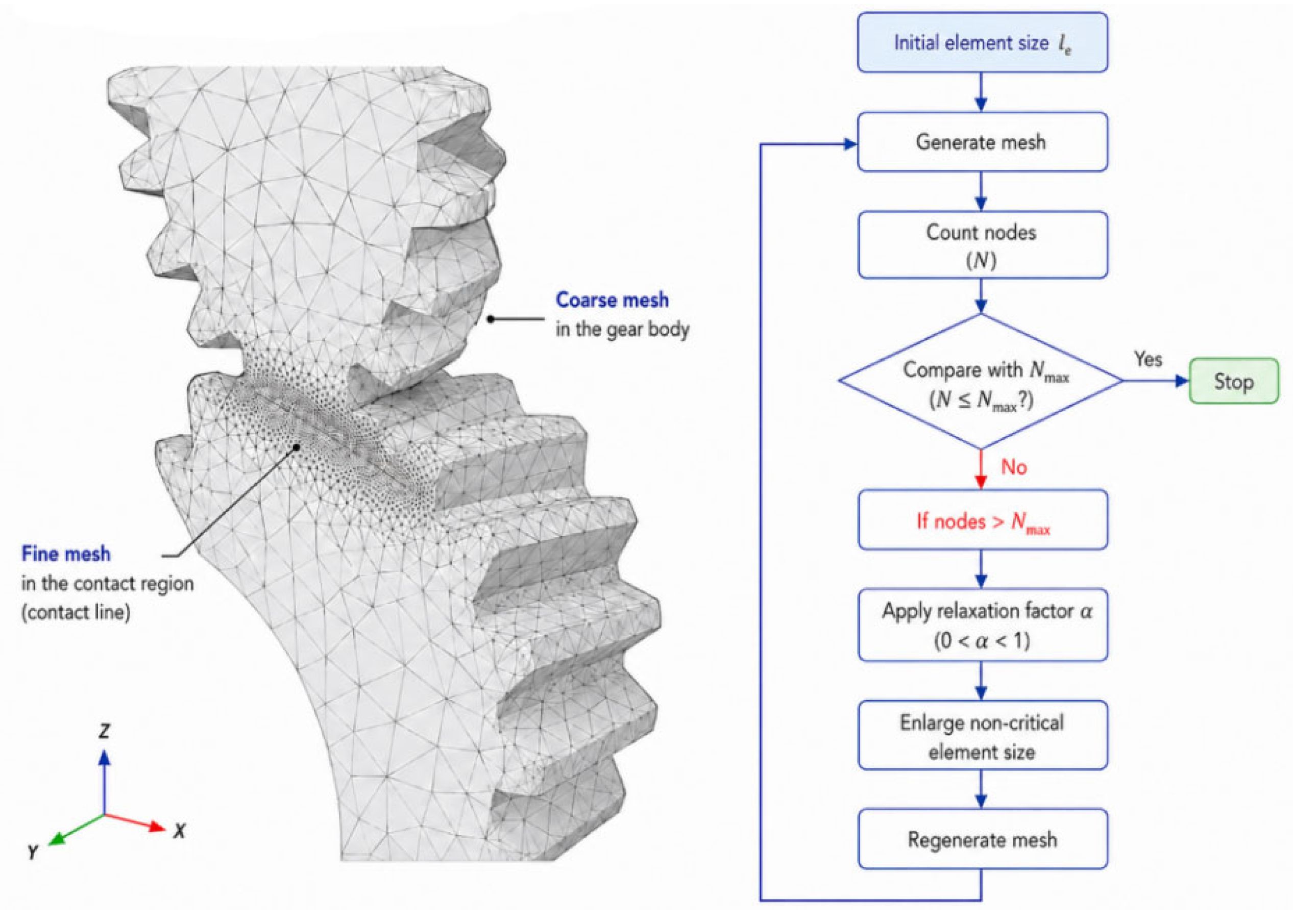
A scripted Ansys/APDL workflow varies gear geometry, torque, angular position, helix angle, misalignment, and material parameters. Each configuration is solved as a separate contact state. The active tooth-flank region receives the smallest elements, whereas the gear body is discretized more coarsely to avoid spending degrees of freedom far from the load path.
Successive meshing states are obtained by advancing the driving gear through the prescribed increment and rotating the driven gear according to the transmission ratio. The resulting positions are passed directly to the contact solver.
The first contact-zone element size is derived from the estimated Hertzian half-width. After meshing, the node count N is compared with the memory-based limit Nmax. If N > Nmax, only the far-field element size and its transition ratio are relaxed; the contact-zone target is kept unchanged. Remeshing continues until the node limit is met (Figure 2).
This feedback rule accepts the first mesh for which N ≤ Nmax. It controls storage without treating contact and far-field regions as equally important, but it is an engineering memory safeguard rather than an error estimator. The archived manuscript record does not retain a transferable numerical Nmax or relaxation increment; those values depend on the available hardware and meshing script. Exact batch regeneration therefore requires release of the corresponding implementation configuration.
Normal contact is enforced with an Augmented Lagrange algorithm. Let gn be the signed normal gap, with gn < 0 denoting interpenetration, and let dn = max(0, −gn) be the nonnegative penetration measure. In Equation (1), pn is the current nonnegative pressure multiplier and εn is the normal penalty stiffness. The multiplier retains the pressure estimate between iterations, while the penalty correction reduces the remaining gap. The positive-part projection prevents tensile normal contact pressure. This formulation reduces penetration without requiring the very large penalty stiffness of a pure-penalty method.
d n k + 1 = m a x 0 , g n k + 1 , p n k + 1 = m a x 0 , p n k + ε n d n k + 1
The active contact set is updated until the program-controlled checks are satisfied; the reported cases maintained normal penetration below 1.0 × 10⁻³ mm. Tangential traction follows Coulomb friction: sticking satisfies ‖tt‖ < μpn and sliding is limited by ‖tt‖ = μpn, with the numerical assumption μ = 0.10. The constitutive model is small-strain linear elasticity. Some calculated local stresses approach the reported yield-strength range of 42CrMo4 steel (approximately 650–930 MPa, depending on heat treatment); these values must therefore be interpreted as elastic-model outputs rather than validated elastoplastic stresses. Plasticity, residual stress, damage, and cyclic hardening are outside the model. Dataset and mesh settings are summarized in Table 1.
The main neural-network training settings are summarized in Table 2 for reproducibility. The table reports the architecture, optimizer, stress scaling, loss weighting, curriculum schedule, sampling strategy, and fixed random seed used in the training implementation.
Training begins with 20 data-only epochs. From epoch 21, the equilibrium weight ramps from zero and reaches its maximum value of 0.5 at epoch 30. Physics nodes are drawn from a coarse-stress importance distribution and capped at 8192 nodes per graph.

2.2. Accelerated Graph Compilation via Hash-Mapped Topologies

Each FE contributes node pairs to the graph. Shared faces and edges cause the same pair to appear repeatedly, so a canonical hash key is assigned to every undirected pair and duplicates are removed before the two message-passing directions are stored [26].
Without deduplication, the graph size reflects element incidence rather than physical connectivity. For example, a 300,000-node mesh can yield more than 15 million raw pair records before repeated pairs are collapsed.
Hash insertion avoids a global comparison of every raw edge with every other edge. Runtime still depends on element type, node ordering, and the hash implementation; no mesh-independent complexity claim is made.
The compiled topology contains one bidirectional edge pair per retained physical adjacency. This step reduces redundant storage before training and is separate from the later fidelity reduction.

2.3. Kdtree Spatial Indexing and Multi-Fidelity Distillation

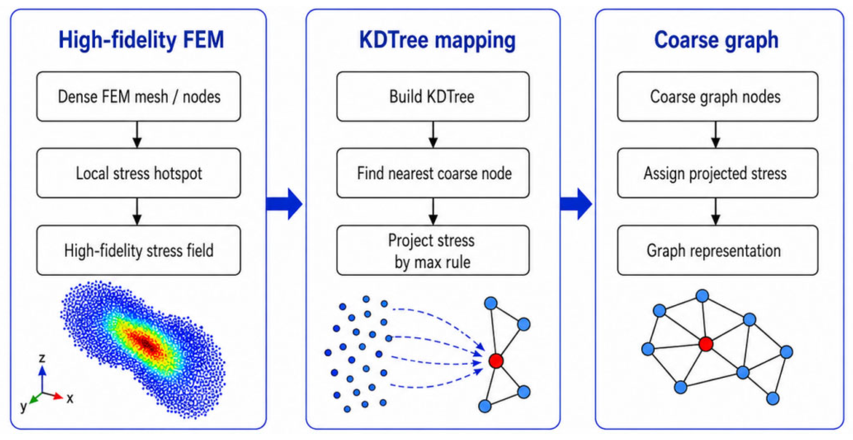
The native FE mesh is dense because accuracy is required near the contact patch, but most of the gear volume carries much smaller stress. Applying every GNN layer to every native node therefore uses memory where little field variation is present. The overall multi-fidelity stress distillation procedure is illustrated in Figure 3.
Uniform coarsening has the opposite defect: it can remove the Hertzian maximum. The adopted representation consequently keeps the fine mesh as the label source and uses a separate, coarser graph for learning.
A KDTree built from coarse-node coordinates assigns every high-fidelity node to its nearest coarse node [27]. The mapping is geometric and fixed for a case. It reduces the learning graph without claiming conservation, continuity, or independence from the chosen coarse resolution.
For a high-fidelity node i at position xi, the nearest receiving coarse node j* is defined by Equation (2). KDTree queries compute this assignment without forming the full fine-by-coarse distance matrix.
j * = arg min j V coarse x i x j 2
After grouping fine nodes by their corresponding coarse node, the source node with the maximum von Mises stress is selected, and its complete six-component Cauchy stress tensor is assigned to that coarse node, as illustrated in Figure 3. Selecting a single physically co-located stress tensor avoids constructing a nonphysical tensor from six independent component-wise maxima. The alternative distance-weighted averaging approach is retained as a controlled sensitivity case, and the corresponding quantitative comparison is detailed in Section 6.5.
Figure 3. KDTree-based peak-sensitive stress projection from the high-fidelity finite element mesh to the coarse learning graph.
Processes 14 02706 g003
The projection separates the FE discretization used to generate labels from the graph on which the network is optimized. Its benefit is the lower graph cost; its price is projection error and dependence on the selected coarse-node density. Because adjacent coarse nodes may inherit tensors from different fine source nodes, the resulting nodal field does not guarantee local C0 continuity or strain-energy conservation. This qualification is important when the equilibrium residual is reconstructed on the same coarse graph and is discussed below.
Related multi-fidelity PINN studies couple information sources [28], transfer representations between fidelity levels [29], or address discontinuous solutions [30]. Here, fidelity reduction is used more narrowly as a peak-sensitive label-transfer operation on an unstructured contact graph.

3. Physics-Guided GatedSAGEConv Network

3.1. Over-Smoothing in Isotropic Aggregation

The surrogate backbone is a five-layer graph network. A conventional GraphSAGE layer forms a permutation-invariant neighborhood mean and combines it with the node’s own state. Equation (3) states this baseline update explicitly.
For node i at layer ℓ, the baseline mean message m i l and updated feature h i l + 1 are
m i l = 1 N i j N i h j l , h i l + 1 = ϕ   W s e l f l h i l + W n e i g h l m i l .
Here, N i is the neighbor set, W s e l f and W n e i g h are learned matrices, and ϕ is the layer nonlinearity. Including the self term makes Equation (3) consistent with the GraphSAGE baseline used in the comparisons.
The mean operator is problematic at a narrow contact boundary. A node inside the loaded patch may exceed 500 MPa while an adjacent node outside the patch is almost unloaded. Their adjacency is geometrically valid, yet unrestricted averaging treats the contrast as noise.
Each additional message-passing layer mixes the peak with a wider low-stress neighborhood.
This progressive homogenization lowers the predicted maximum and broadens the apparent contact zone, the characteristic over-smoothing failure for this task.
A field with low global error can therefore remain unsuitable for fatigue calculations if it misses the local maximum.

3.2. Physical Gating Mechanism

The proposed GatedSAGEConv retains the five-layer, 128-channel backbone but multiplies each incoming neighbor message by a learned scalar gate before mean aggregation. A residual path, SiLU activation, dropout, and LayerNorm complete each layer.
The gate is intended to reduce exchange across edges with a strong contrast in the coarse stress prior while preserving communication within a similar stress regime. It is a learned weighting function and does not impose an exact traction-jump condition.
The full gate uses coarse projected stress derived from the same high-fidelity field that supplies the target, so the conditioned benchmark receives target-related information and must not be described as label-free inference. To quantify this dependence, a geometry-only gate using distance and element-quality features was evaluated for seed 42. Its peak-stress error was 4.1%, compared with 2.3% for the stress-prior-conditioned model and 15.6% for the no-gate ablation. This geometry-only result is preliminary because its full NMSE, R2, memory, and multi-seed uncertainty were not retained.
Evaluation Protocols: The full-model metrics in Table 3, Table 4 and Table 5 use the projected stress prior and are reported as stress-prior-conditioned numerical benchmarks. A predicted-prior two-pass route could first generate a coarse stress estimate and then use it to form gate features, but no separately documented first-pass model, end-to-end accuracy, or end-to-end timing were retained. This is therefore a future deployment hypothesis, not a validated result. The geometry-only gate requires no stress prior and is the only explicitly label-free inference result reported here.
For edge (i,j), the gate receives the two latent node states and three scalar descriptors: normalized distance Δxij, absolute prior-stress contrast Δsij, and prior-stress product Πij. The prior s is a nonnegative scalar equivalent stress and is distinct from the predicted six-component tensor.
Geometric Scale: Equation (4) divides the Euclidean separation of connected nodes by the graph’s mean edge length ¯ , giving a dimensionless gate input.
Δ x i j = x i x j 2 l ¯
Prior Contrast: Equation (5) is nonnegative and becomes large when an edge joins dissimilar coarse equivalent-stress regimes.
Δ s i j = | s i p r i o r s j p r i o r |
Prior Co-Activation: Equation (6) distinguishes two jointly loaded nodes from a loaded-to-unloaded pair. It is an input feature only and should not be interpreted as strain-energy density. The archived record does not retain any additional scaling applied to Δsij and Πij; exact reproduction of gate-input preprocessing therefore requires the implementation configuration.
Π i j = s i p r i o r s j p r i o r
The descriptors and latent states are concatenated and passed through a gate MLP followed by a sigmoid (Equation (7)), so each edge weight lies between zero and one.
e i j l = s i g m o i d M L P g a t e h i l h j l Δ x i j Δ s i j Π i j
Equation (8) gives the implemented gated mean and residual update. Because eij is scalar, it scales the neighbor vector; no elementwise gate tensor is implied.
m i l = 1 N i j N i e i j l W n e i g h l h j l , h i l + 1 = L a y e r N o r m h i l + D r o p o u t S i L U W s e l f l h i l + m i l .
The residual branch supplies an unattenuated path for the node state, while LayerNorm and dropout stabilize optimization across the five layers.
A small gate suppresses, rather than deletes, a message crossing a steep prior-stress contrast. The network can still learn to pass information when the latent states and geometry support it.
Mesh-based mechanics surrogates include hierarchical physics-informed MeshGraphNets [31] and multilevel graph models for structural dynamics [32]. Their hierarchy and time-dependent settings differ from the single coarse graph and static equilibrium problem considered here. A posteriori error indicators [33] could provide complementary reliability screening, but they do not directly solve peak preservation at a gear-contact boundary.
Related graph and PINN studies encode geometric boundary information, predict urban flow on unstructured meshes [34], reconstruct finite-strain mechanical fields [35], integrate graph-informed neural ordinary differential equations [36], or embed symmetry constraints [37]. These examples show the breadth of physics-guided learning, but they do not provide experimental validation for the present contact projection and gate.
The full gate described below uses the projected coarse stress prior, which is derived from the same high-fidelity FE solution that provides the training labels. Therefore, the conditioned model is not label-free. To quantify the benefit of removing target information, we also evaluate a geometry-only gate that replaces Δs and Π with edge-based geometric features (edge length and local curvature estimate). Its performance is reported separately in Section 6.

4. Physics-Constrained Optimization

The predictive accuracy and physical consistency of the proposed gear surrogate are supported by a composite objective that combines data-driven regression with continuum-mechanics constraints. The formulation is evaluated on the reported 96 GB GPU configuration [38].
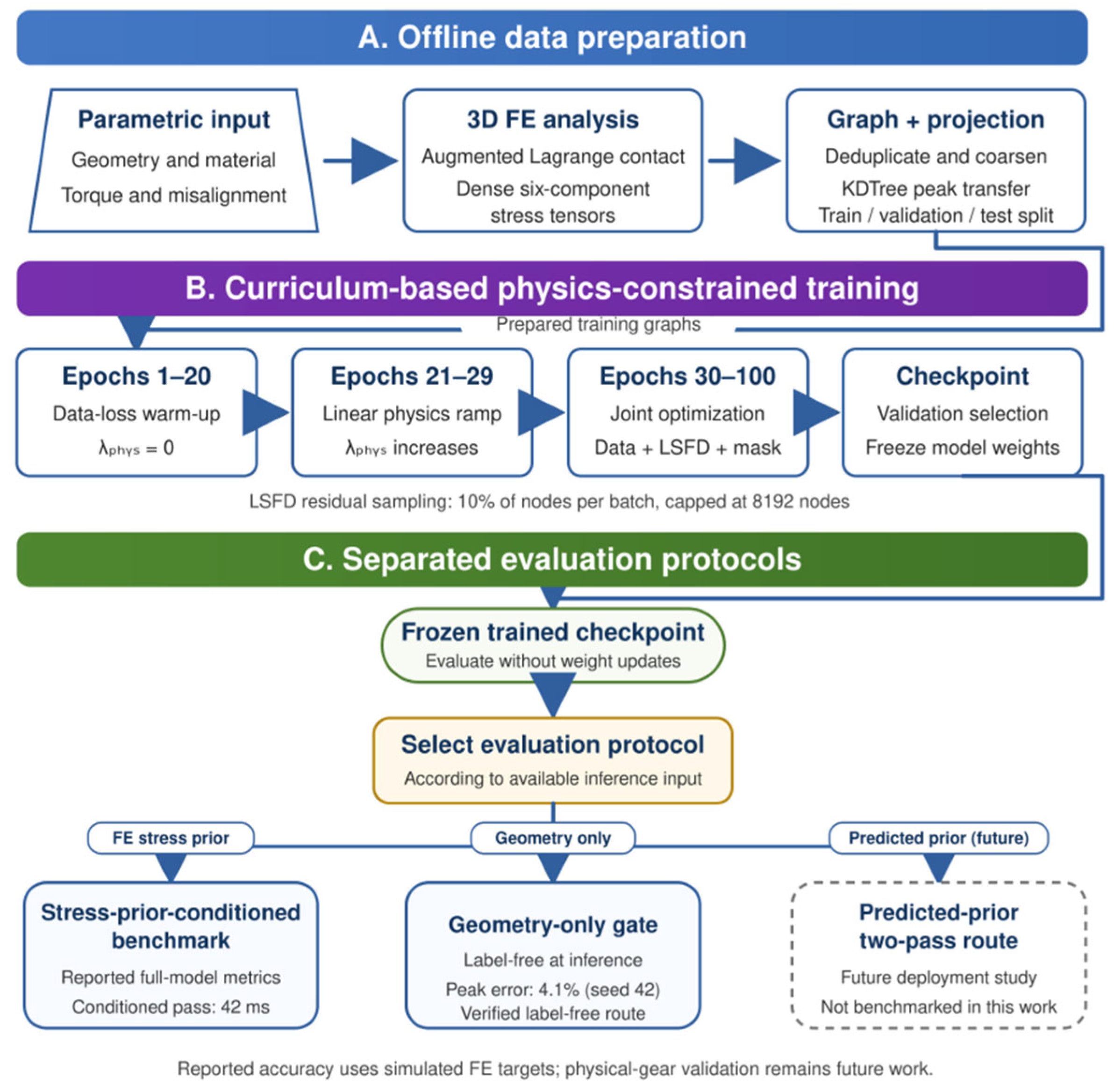
For clarity, Figure 4 summarizes the framework in three stages. During offline data preparation, parametric inputs are evaluated through 3D FE contact analysis, after which the resulting stress tensors are transferred to coarse graphs using peak-sensitive projection and divided into training, validation, and test sets. During curriculum-based physics-constrained training, the model is optimized using the data, LSFD physics, and masking losses according to the prescribed schedule, with checkpoint selection based exclusively on the validation data. Evaluation is subsequently performed with frozen model weights under two reported protocols: the stress-prior-conditioned benchmark and the preliminary geometry-only route. In the diagram, the phrase ‘verified label-free route’ means only that the geometry-only configuration was executed for seed 42 and yielded a retained peak-error value of 4.1%; it does not denote complete multi-seed or experimental verification. The predicted-prior two-pass route is prospective work and was not benchmarked in this study.

4.1. Data-Driven Loss with Log-Stress Normalization

The network predicts the six independent components of the symmetric Cauchy stress tensor. These components have a strongly imbalanced distribution: most nodes are lightly loaded, whereas a small contact region contains the largest magnitudes.
A direct component-wise MSE can be dominated by the numerous low-stress nodes. Moreover, the shear components can be negative, so ln(1 + ασ) is not defined over the full target range. We therefore use the sign-preserving transform T s , with σ 0 = 10 M P a , applied separately to all six components.
The data term is the mean squared distance between the transformed prediction and reference tensors:
T s = s g n s l n 1 + s σ 0 , σ 0 = 10 M P a , L d a t a = 1 6 V i V T σ ^ i T σ i F E 2 2
The transformation is dimensionless, preserves the sign of shear stress, and compresses the dynamic range without discarding the peak-bearing samples.

4.2. Memory Requirements of Autograd-Based Pinn

Physics supervision is introduced through the local equilibrium of the predicted Cauchy stress.
For static or quasi-static small-strain motion, the balance of linear momentum reduces to Equation (10); f is body force per unit volume and is zero in the reported simulations.
σ + f = 0
Equation (11) lists the three Cartesian components. Stress symmetry (σxy = σyx, σxz = σzx, and σyz = σzy) leaves six independent output components.
σ x x x + σ x y y + σ x z z + f x = 0 σ y x x + σ y y y + σ y z z + f y = 0 σ z x x + σ z y y + σ z z z + f z = 0
Coordinate automatic differentiation is inexpensive for a pointwise multilayer perceptron because each output depends only on its own coordinate. In a message-passing graph, however, a node output also depends on features collected from neighboring coordinates.
Differentiating equilibrium through an L-layer GNN therefore traverses an L-hop receptive field. An upper-bound count of paths grows as O(d^L) for average degree d, although the repeated nodes mean this is not an exact memory-complexity identity.
In the reported million-node, five-layer test, the coordinate-AD residual variant produced an out-of-memory failure on the 96 GB GPU. The profiler/allocation record projected demand above 100 GB; this is an estimate associated with the failed run rather than a directly measured peak. The observation motivates an output-space derivative approximation but does not establish a universal limit for all AD implementations.
The bottleneck is consequently specific to full-graph training at the stated resolution and hardware.
The constitutive reference is linear elastic 42CrMo4 steel. Predictions near the reported yield interval remain comparable to the elastic FE model; plastic flow, residual stress, damage, and cyclic hardening are outside the governing equations used here.

4.3. Unstructured Finite Difference Gradient Reconstruction

Spatial derivatives are reconstructed from the final predicted field and the fixed graph geometry. This is a weighted least-squares finite-difference calculation, not a derivative of the network with respect to its input coordinates.
For each node, neighboring output differences supply an overdetermined local system for the three spatial derivatives of each of the six stress components.
For component q and neighbor j, the first-order Taylor relation is written in Equation (12):
σ q , j σ q , i x j x i T σ q x i , q = 1 , , 6
Stacking all neighbor relations yields Equation (13). The rows of Ai are three-dimensional coordinate offsets, the six columns of Gi are component gradients, and the matching rows of ΔΣi are stress differences. The matrix dimensions are stated directly in the following equation:
A i G i Δ Σ i , A i R n i × 3 , G i R 3 × 6 , Δ Σ i R n i × 6
The regularized weighted least-squares solution is given by Equation (14). For each one-ring neighbor j, the diagonal weight is Wij = (‖xj − xi2 + ε)ᵖ with inverse-distance exponent p = 1. The stencil contains all deduplicated one-ring graph neighbors; no additional global Euclidean cutoff is applied. Its effective radius is ri = maxj∈N(i) ‖xj − xi2 and varies with the mesh. The term ηI3 regularizes a singular or poorly conditioned local normal matrix. The archived experiment record retains p and the stencil definition but not the numerical values of η and ε; exact pointwise residual reproduction is therefore not claimed until those implementation constants are recovered.
G i = A i T W i A i + η I 3 1 A i T W i Δ Σ i
The regularization improves numerical conditioning but does not guarantee consistency for an arbitrary degenerate neighborhood. Nodes with fewer than three independent offset directions must therefore be excluded, expanded to a larger stencil, or solved with a pseudoinverse [39].
The dense-to-coarse mesh transition uses the same one-ring stencil. Inverse-distance weighting reduces the leverage of longer transition edges, but abrupt changes in edge length and anisotropic neighbor directions can still increase first-order reconstruction error. The regional prediction errors reported later do not isolate this LSFD truncation error, and no manufactured-solution or stencil-refinement test was performed. Accordingly, transition-zone gradient accuracy is treated as a numerical limitation rather than an independently validated claim.
To control cost, the residual is evaluated on a subset biased toward large coarse stress and steep coarse gradients. The sampling fraction is 10% and is capped at 8192 nodes; far-field nodes remain represented by the separate mask term.
The dimensionless equilibrium penalty is as follows:
In Equation (15), r 0 = σ r e f / L r e f is the residual scale induced by the stress and coordinate normalization, so the physics term is dimensionless before it is combined with the data and mask losses.
L p h y s = 1 S s a m p l e k S s a m p l e F D σ ^ k + f k r 0 2 2
Related work has combined physics-informed GNNs with finite-difference residuals on unstructured spatiotemporal PDEs [24] and developed graph–Galerkin formulations [40]. The present method instead reconstructs static stress gradients from fixed one-ring output differences. This reduces coordinate–AD graph retention but does not remove truncation, conditioning, or sampling error.
Neural-FEM and neural-operator comparisons in solid mechanics clarify representation and training tradeoffs [41], while physics-informed super-resolution [42], residual correction [43], and distributed operator learning [44] offer complementary routes. These methods are relevant baselines for future common-budget tests, but they do not by themselves validate the present fixed-resolution contact graph.

4.4. Projection-Induced Discontinuities and Residual Interpretation

The physics loss remains algebraically well-defined because the maximum-projected label and the predicted field each store one finite stress tensor at every coarse node. The Taylor reconstruction in Equation (14), however, assumes a locally smooth field. A jump created when adjacent receiving nodes select source tensors from opposite sides of an assignment or contact–void boundary therefore enters the reconstructed divergence together with the physical stress gradient. A localized residual peak at such a boundary is not, by itself, proof of violated continuum equilibrium.
A region-tagged residual map and a matched LSFD–automatic-differentiation subgraph comparison were not performed. The physics loss is therefore interpreted as a regularizer rather than strict enforcement of continuum equilibrium; the curriculum keeps the data loss dominant while the gross field is forming.
During training, Equation (15) is evaluated on the network prediction rather than on the projected label. The data term pulls the prediction toward the peak-preserving target, whereas the physics term discourages non-equilibrated local differences; delaying the latter creates a discretization–regularization tradeoff but does not restore C0 continuity or energy conservation to the projection. Full-graph coordinate automatic differentiation failed because of out-of-memory demand, so Table 4 reports no AutoGrad accuracy values and no pointwise matched residual comparison. Region-tagged residual maps and tractable matched-subgraph checks remain for future reproducibility work.

4.5. Non-Contact Spatial Mask Loss

Small nonzero predictions can persist in the nominally unloaded gear body. Although these values have little influence on global MSE, they can contaminate field integrals.
A far-field set is defined through its distance to the theoretical line of action, using the chosen multiple of the characteristic contact half-width. This criterion approximates the decay of elastic half-space solutions and is not an exact traction-free boundary condition.
The binary mask MSV,i equals one only for nodes in this far-field set. Equation (16) penalizes their predicted stress norm.
L m a s k = 1 | V f a r | i V M S V , i σ ^ i 2 2

5. Temporal Curriculum Learning

Applying the equilibrium term at full strength to an untrained field produced unstable early gradients.
The objective therefore uses a fixed mask coefficient and an epoch-dependent physics coefficient (Equation (17)).
L t o t a l = L d a t a + λ m a s k L m a s k + λ p h y s t L p h y s
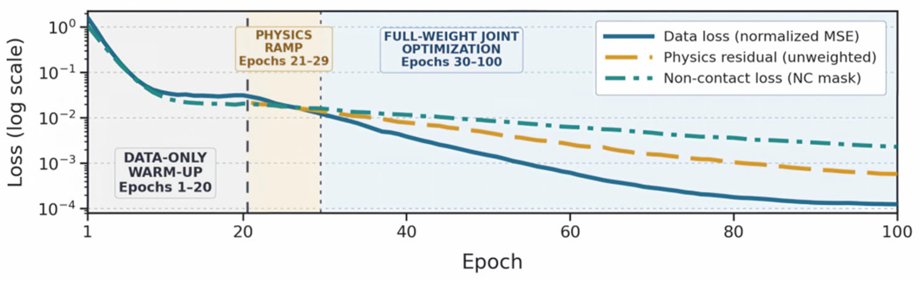
The mask coefficient is λmask = 0.02. The physics coefficient λphys(t) is zero for epochs 1–20, ramps during epochs 21–29, and equals 0.5 from epoch 30 onward, matching Table 2. This schedule lets the network establish the gross stress field before equilibrium residuals refine local gradients [45,46,47].
Figure 5 is a schematic visualization of the piecewise curriculum specified in Table 2: the physics coefficient is zero during epochs 1–20, increases linearly during epochs 21–29, and remains at its maximum value of 0.5 from epoch 30 through epoch 100. The three plotted loss trajectories were generated from synthetic illustrative values to show the intended relative behavior of the data, physics-residual, and non-contact terms. They are not a retained per-epoch training history and therefore are not used to claim empirical convergence, compare optimization rates, or select the reported checkpoint. Quantitative performance claims are based on the retained metrics in Table 4, Table 5 and Table 6.

6. Results and Discussion

The numerical evaluation addresses component ablation, comparison with internal baselines, field error, peak preservation, and computational cost. Every reference field in this section is produced by the same FE pipeline, as described above.

6.1. Ablation Study and Baseline Comparison

The Ours-Full row in Table 4 and the test row in Table 6 report the same mean ± standard deviation over five random seeds (37, 42, 55, 73, and 91). Table 5 retains the seed-42 internal baseline comparison. Other ablation variants are seed-42 results unless the table states otherwise; only the geometry-only peak-stress error was retained for that variant.
Table 5 includes GCN + Prior, a five-layer GCN augmented with the same projected stress-prior feature used by the conditioned proposed model. This provides an information-matched comparison for assessing the additional effect of the gated architecture and associated training design.
The stress-prior-conditioned configuration has the lowest reported peak error among the tested variants. This comparison does not isolate graph resolution, because every variant uses the same coarse-node count, and it must be read together with the geometry-only result and target-information limitation.
Table 5 uses baselines implemented on the same numerical dataset and test split. All models are trained with the same data, and those with a prior input (GCN + Prior and Ours) receive the projected coarse stress prior as an additional feature. The proposed stress-prior-conditioned model has 196,680 parameters, or 1.76× the 111,560-parameter GCN, so the GCN comparison alone does not isolate architecture from capacity. GraphSAGE is the nearest capacity-aligned baseline at 194,120 parameters (1.3% fewer than the proposed model), yet its NMSE and peak-stress error remain 2.61 × 10⁻⁴ and 14.2%, respectively. The no-gate ablation retains the five-layer, 128-channel backbone and training configuration while removing the physical edge gate; its peak-stress error is 15.6%. These controls suggest that parameter count alone is insufficient to explain the conditioned result, but they do not remove the stress-prior information advantage.
The GCN + Prior baseline closes much of the gap, indicating that prior information materially contributes. The proposed model still improves the seed-42 peak-stress error from 5.8% to 2.3% and lowers NMSE. Because both conditioned models receive the same peak-projected prior, the remaining difference is consistent with the gated architecture and associated training design; it cannot be attributed to prior availability or projection alone.
An exactly parameter-matched GCN and a documented equal hyperparameter-search budget were not included; accordingly, no strict capacity-controlled ranking is claimed. FNO-, PI-MGN-, and DeepONet-style models would also require additional representation and memory choices for this unstructured contact mesh. A common-dataset, common-budget comparison with neural operators and hierarchical mesh solvers remains necessary to separate the benefit of the gate from the benefit of the chosen representation.
Table 4 and Table 6 report the same five-seed test summary for the conditioned full model: NMSE = (9.1 ± 0.4) × 10−5, R2 = 0.985 ± 0.001, and peak-stress error = 2.5 ± 0.2%. Table 4 retains the seed-42 comparison values of 8.7 × 10⁻⁵, 0.985, and 2.3%.

6.2. Numerical Stress-Field Accuracy

Table 6 reports the retained split-level metrics. The test row gives the five-seed mean ± standard deviation; the training and validation rows are single retained summary values.
The sampled interpolation envelope is module 2.0–4.5, tooth count 18–120, torque 100–480 N·m, helix angle 0–25°, and misalignment 0–0.30°. Extrapolation, material transfer, and non-standard tooth-profile transfer were not evaluated. Moreover, the archived split record retains case counts and ratios but does not document grouping by parent gear geometry or adjacent angular state. Potential near-neighbor leakage cannot be excluded; future validation should use grouped holdouts before stronger generalization claims.

Peak Stress Preservation

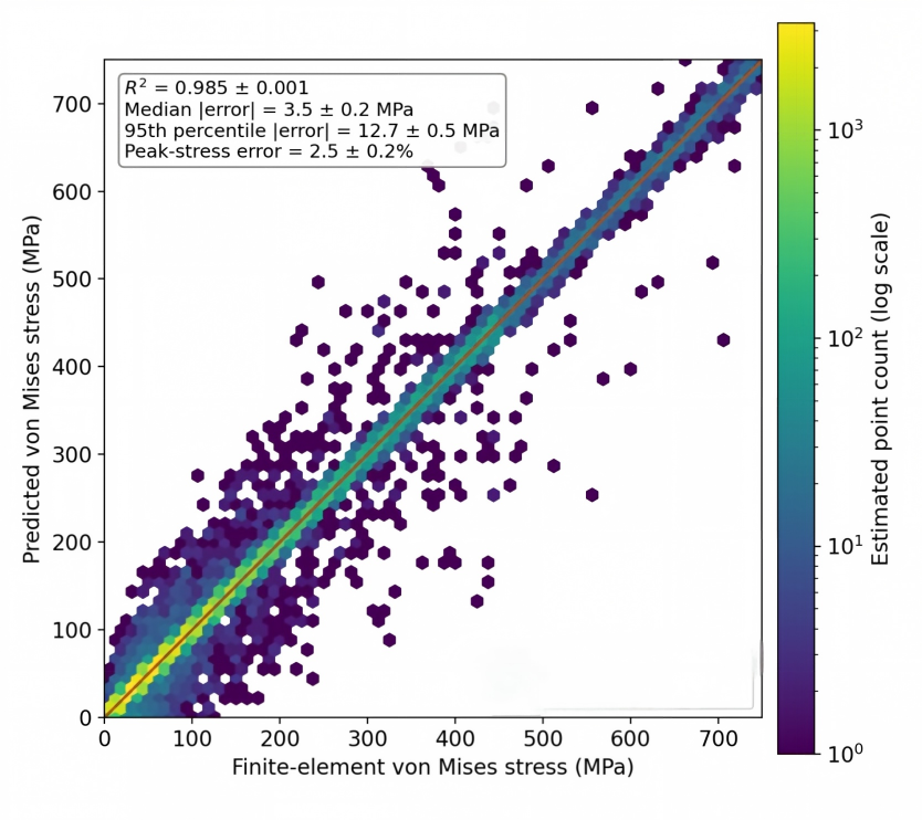
Peak accuracy is compared numerically in Table 4, Table 5 and Table 6. For seed 42, the GCN, GraphSAGE, and no-gate models report peak-stress errors of 17.6%, 14.2%, and 15.6%, respectively, whereas the conditioned proposed model reports 2.3%. Across five seeds, the retained test-split value is 2.5 ± 0.2%; the geometry-only gate gives 4.1% for seed 42 only. Figure 6 is not generated from retained raw point-level prediction/reference pairs. It is a density-binned reconstruction based on 604 occupied hexagonal-bin centers and estimated counts recovered from the available plot. The five-seed statistics displayed in its inset are the retained summary values from Table 6, rather than statistics recomputed from raw plotted samples. The figure is therefore descriptive and does not independently validate spatial consistency or the tabulated metrics.
As a reconstruction check, weighting the recovered bin centers by the estimated rounded counts gives R2 = 0.982, RMSE = 22.8 MPa, MAE = 16.9 MPa, and a fitted slope of 0.999. These bin-level approximations are not interchangeable with the five-seed statistics in Table 6 because the underlying aggregation and source records differ. Accordingly, Figure 6 is used only to display the approximate agreement pattern; the tabulated experiments, rather than the reconstructed plot alone, support the numerical comparison. Neither the figure nor the tables establish fatigue-life accuracy, because no material S–N calibration, cumulative-damage model, or experimental life measurement was evaluated.
Accordingly, the peak-error result is presented as a numerical stress-surrogate metric rather than a direct prediction of crack initiation, pitting life, or field failure risk.

6.3. Inference Latency and Scope

The reference FE solve averaged 4.5 h on a 64-core HPC cluster for a case with approximately 1 × 10⁶ native nodes. This value characterizes the stated solver setup; differences in hardware, software, convergence tolerances, and preprocessing prevent a strictly normalized solver-to-network speed comparison.
The reported 42 ms value is the latency of one forward pass on the coarse graph when the stress prior and graph tensors are already available. It excludes FE generation, graph compilation, host-to-device transfer, construction of a label-free prior, and any preliminary pass required by a predicted-prior scheme.
The FE time and conditioned forward-pass time therefore provide a kernel-level numerical contrast, not a measured end-to-end deployment speedup. Real-time monitoring, control, and digital-twin use require separate validation of the input pipeline, label-free gating, uncertainty, and experimental accuracy.

6.4. Memory Profile

For the coordinate-AD ablation, full-graph training failed with an out-of-memory error on the 96 GB GPU, and the allocation estimate exceeded 100 GB. Because the run was not completed, the >100 GB value in Table 4 is an estimate rather than a measured peak and should not be generalized to all PINN or AD implementations.
With fixed-topology LSFD reconstruction and importance sampling, the conditioned full model completed training with a measured peak of 47.6 GB. This memory value is specific to the approximately 5 × 10⁵-node coarse graph, batch size one, five-layer architecture, numerical precision, and reported software/hardware configuration.
Table 6 separates measured values from estimates and failed runs. The FE memory peak was not reported. The point-cloud PINN row records an out-of-memory result and projected demand rather than a completed latency measurement. The proposed row reports 47.6 GB training peak memory and 42 ms for one stress-prior-conditioned forward pass; neither value is an end-to-end label-free deployment measurement.
The reconstructed residual approximates equilibrium on the selected graph stencil. Its accuracy depends on neighbor geometry, regularization, normalization, and sampling; near a maximum-projection boundary, it can also contain a projection-induced jump component. It is therefore not proof of exact satisfaction of the continuous PDE.

6.5. Projection-Strategy Sensitivity and Graph-Resolution Limits

The projection-strategy check changes only the aggregation rule while retaining the dataset, coarse graph, network, and training protocol. For coarse control volume i, the complementary-energy error uses e i = σ i p r e d σ i r e f , compliance S = C 1 , and volume weight Vi; the normalized metric is the square root of ε E = i V i e i S e i i V i ( σ i r e f ) S σ i r e f 1 / 2 . This is a post-training comparison metric on the matched coarse representation; it is neither a proof of maximum-projection convergence nor evidence that the projection restores continuity. Table 7 reports the metric under the stated validation protocol.
Relative to distance-weighted averaging, maximum projection lowers coarse-grid NMSE from 1.18 × 10⁻⁴ to 8.87 × 10⁻⁵ (24.8%), peak-stress error from 3.1% to 2.3% (25.8%), and complementary-energy error from 2.8% to 2.1% (25.0%). This supports the choice of projection rule under one fixed graph density. It is not a graph-construction sensitivity study: only the approximately 5 × 10⁵-node coarse graph was trained. A node-count or neighborhood-radius sweep is required before claiming resolution robustness.

6.6. Numerical Validation Scope and Experimental Requirements

All 5000 cases, including the training, validation, and test splits, were generated by Ansys using one contact formulation and the parameter ranges in Table 1. Consequently, the reported errors quantify surrogate agreement with that numerical model. They do not establish accuracy against a physical gear, nor do they capture model-form uncertainty in friction, lubrication, surface roughness, heat treatment, manufacturing deviations, or elastoplastic response.
Experimental validation should use an instrumented gear test rig with independently measured torque, alignment, geometry, material state, and flank temperature. Strain or contact-pressure measurements should be reserved as a blind test after uncertain FE parameters are calibrated on separate cases. Until such data are available, the method is presented as a fast FE surrogate for numerical screening, not as a validated digital-twin replacement for condition monitoring.
Dynamic tooth-fault models for split-torque and planetary transmissions provide a natural system-level interface for future validation: the local stress surrogate could be coupled to time-varying mesh stiffness, load-sharing, and vibration calculations, and then tested against rig measurements. That coupling is not part of the present simulated-data study.

7. Conclusions

This study developed a peak-sensitive graph surrogate for six-component 3D gear-contact stress. Under the stress-prior-conditioned benchmark, the held-out test split yields an NMSE = (9.1 ± 0.4) × 10−5, R2 = 0.985 ± 0.001, and peak-stress error = 2.5 ± 0.2% across five seeds. The preliminary geometry-only gate reports 4.1% peak error for seed 42. At the tested graph resolution, peak training memory is 47.6 GB and one conditioned forward pass takes 42 ms. The fixed-resolution projection comparison favors maximum transfer over distance-weighted averaging.
The conclusions are limited in seven ways. First, coarse-graph resolution was not swept, so projection and graph-density errors cannot be separated. Second, numerical LSFD values for η and ε, a region-tagged residual map, and a matched LSFD–AD subgraph check were not retained in the archived record; recovery and systematic archiving of these constants is currently underway as part of an ongoing engineering reproducibility effort. Third, the headline metrics are stress-prior-conditioned; complete multi-seed geometry-only metrics and end-to-end predicted-prior results remain unavailable. Fourth, the archived split record does not document grouping by parent geometry or adjacent angular state, so near-neighbor leakage cannot be excluded. Fifth, exact gate-input scaling and complete hardware/software identifiers were likewise not retained and are being recovered alongside η and ε. Sixth, every target is simulated, so experimental accuracy is unknown. Seventh, the curves in Figure 5 are synthetic illustrations and the hexagonal bins in Figure 6 are reconstructed estimates; neither figure constitutes an independent raw-data benchmark. Engineering implementation work is ongoing, including instrumented rig preparation and integration with transmission-level dynamic models. Future work will recover the missing configuration, perform grouped and resolution-sensitive validation, and conduct blind rig tests with more realistic contact physics.

Author Contributions

Conceptualization, Q.L.; methodology, J.Z. and Q.L.; software, Z.L.; validation, J.Z., Z.L. and Q.L.; formal analysis, J.Z., Z.L. and Q.L.; investigation, Z.L. and Q.L.; data curation, J.Z., Z.L. and Q.L.; writing—original draft preparation, J.Z. and Q.L.; writing—review and editing, Q.L.; visualization, Z.L.; supervision, Q.L.; funding acquisition, Q.L. All authors have read and agreed to the published version of the manuscript.

Funding

This research was funded by the Industry–University–Research Cooperation Project of Ruian City, Zhejiang Province (project: Research on Adaptive Finite Element Analysis and Error Optimization Technology for Gear Design Based on AI Agent; Contract No. 2025110143HX).

Data Availability Statement

The finite-element simulation data and processed graph datasets supporting the findings of this study are available from the corresponding author upon reasonable request. The synthetic curriculum values used to construct Figure 5 and the reconstructed hexagonal-bin table used for Figure 6 are also available on request. No experimental or third-party datasets were used.

Conflicts of Interest

The authors declare no conflicts of interest.

References

  1. Yang, X.; Yin, S.; Chen, Y.; Zhang, Y.; Zhang, S.; Wu, Y. Numerical and experimental research of helical gear contact stress considering the influence of friction. Front. Mech. Eng. 2022, 8, 1078134. [Google Scholar] [CrossRef] [Scilit]
  2. Yang, Y.; Qiu, D.; Hu, N.; Hu, J.; Zhang, L.; Cheng, Z. Dynamic modeling and analysis of a split-torque transmission with a tooth crack fault. Nonlinear Dyn. 2026, 114, 148. [Google Scholar] [CrossRef] [Scilit]
  3. Yang, Y.; Hu, N.; Li, Y.; Cheng, Z.; Shen, G. Dynamic modeling and analysis of planetary gear system for tooth fault diagnosis. Mech. Syst. Signal Process. 2024, 207, 110946. [Google Scholar] [CrossRef] [Scilit]
  4. Sugunesh, A.P.; Mertens, A.J. A comprehensive study on Hertzian contact stress behaviour of engineering thermoplastic gears using 3D finite element analysis. Proc. Inst. Mech. Eng. Part C J. Mech. Eng. Sci. 2024, 238, 586–597. [Google Scholar] [CrossRef] [Scilit]
  5. Bonari, J.; Paggi, M.; Dini, D. A new finite element paradigm to solve contact problems with roughness. Int. J. Solids Struct. 2022, 253, 111643. [Google Scholar] [CrossRef] [Scilit]
  6. Gapp, S.; Otipka, D.; Maierhofer, J.; Daves, W.; Antretter, T. Efficient 3D finite element modeling of elasto-plastic Hertzian contact of two crossed cylinders with varying contact ellipses after high cycles. Tribol. Int. 2025, 211, 110825. [Google Scholar] [CrossRef] [Scilit]
  7. Bruzzone, F.; Fabbri, D.; Rosso, C. Machine learning surrogate models for Hertzian contact stress prediction in gear design: A comparative study of multiple approaches. Next Res. 2025, 2, 100940. [Google Scholar] [CrossRef] [Scilit]
  8. Gladstone, R.J.; Rahmani, H.; Suryakumar, V.; Meidani, H.; D’Elia, M.; Zareei, A. Mesh-based GNN surrogates for time-independent PDEs. Sci. Rep. 2024, 14, 3394. [Google Scholar] [CrossRef] [Scilit] [PubMed]
  9. Rusch, T.K.; Bronstein, M.M.; Mishra, S. A survey on oversmoothing in graph neural networks. arXiv 2023, arXiv:2303.10993. [Google Scholar] [CrossRef] [Scilit]
  10. Li, H.; Miao, Y.; Sharif Khodaei, Z.; Aliabadi, M.H. Finite-PINN: A physics-informed neural network with finite geometric encoding for solid mechanics. J. Mech. Phys. Solids 2025, 203, 106222. [Google Scholar] [CrossRef] [Scilit]
  11. He, W.; Li, J.; Kong, X.; Deng, L. Multi-level physics informed deep learning for solving partial differential equations in computational structural mechanics. Commun. Eng. 2024, 3, 151. [Google Scholar] [CrossRef] [Scilit] [PubMed]
  12. Oono, K.; Suzuki, T. Graph neural networks exponentially lose expressive power for node classification. In Proceedings of the International Conference on Learning Representations (ICLR), Addis Ababa, Ethiopia, 26–30 April 2020; Available online: https://openreview.net/forum?id=S1ldO2EFPr (accessed on 1 January 2026).
  13. Li, Z.; Kovachki, N.; Azizzadenesheli, K.; Liu, B.; Bhattacharya, K.; Stuart, A.; Anandkumar, A. Fourier neural operator for parametric partial differential equations. In Proceedings of the International Conference on Learning Representations (ICLR), Virtual Event, Austria, 3–7 May 2021; Available online: https://openreview.net/forum?id=c8P9NQVtmnO (accessed on 1 January 2026).
  14. Lu, L.; Jin, P.; Pang, G.; Zhang, Z.; Karniadakis, G.E. Learning nonlinear operators via DeepONet based on the universal approximation theorem of operators. Nat. Mach. Intell. 2021, 3, 218–229. [Google Scholar] [CrossRef] [Scilit]
  15. Pathak, J.; Subramanian, S.; Harrington, P.; Raja, S.; Chattopadhyay, A.; Mardani, M.; Kurth, T.; Hall, D.; Li, Z.; Azizzadenesheli, K.; et al. FourCastNet: A global data-driven high-resolution weather model using adaptive Fourier neural operators. arXiv 2022, arXiv:2202.11214. [Google Scholar] [CrossRef] [Scilit]
  16. Bai, J.; Jeong, H.; Batuwatta-Gamage, C.P.; Xiao, S.; Wang, Q.; Rathnayaka, C.M.; Alzubaidi, L.; Liu, G.-R.; Gu, Y. An introduction to programming Physics-Informed Neural Network-based computational solid mechanics. Int. J. Comput. Methods 2023, 20, 2350013. [Google Scholar] [CrossRef] [Scilit]
  17. Jagtap, A.D.; Kawaguchi, K.; Karniadakis, G.E. Adaptive activation functions accelerate convergence in deep and physics-informed neural networks. J. Comput. Phys. 2020, 404, 109136. [Google Scholar] [CrossRef] [Scilit]
  18. Shin, Y.; Darbon, J.; Karniadakis, G.E. On the convergence of physics informed neural networks for linear second-order elliptic and parabolic type PDEs. Commun. Comput. Phys. 2020, 28, 2042–2074. [Google Scholar] [CrossRef] [Scilit]
  19. Pfaff, T.; Fortunato, M.; Sanchez-Gonzalez, A.; Battaglia, P.W. Learning mesh-based simulation with graph networks. In Proceedings of the International Conference on Learning Representations (ICLR), Virtual Event, Austria, 3–7 May 2021; Available online: https://openreview.net/forum?id=roNqYL0_XP (accessed on 1 January 2026).
  20. Li, Z.; Kovachki, N.; Azizzadenesheli, K.; Liu, B.; Bhattacharya, K.; Stuart, A.; Anandkumar, A. Multipole graph neural operator for parametric partial differential equations. Adv. Neural Inf. Process. Syst. 2020, 33, 6755–6766. [Google Scholar]
  21. Defferrard, M.; Bresson, X.; Vandergheynst, P. Convolutional neural networks on graphs with fast localized spectral filtering. Adv. Neural Inf. Process. Syst. 2016, 29, 3844–3852. [Google Scholar]
  22. Chen, J.; Ma, T.; Xiao, C. FastGCN: Fast learning with graph convolutional networks via importance sampling. In Proceedings of the International Conference on Learning Representations (ICLR), Vancouver, BC, Canada, 30 April–3 May 2018; Available online: https://openreview.net/forum?id=rytstxWAW (accessed on 1 January 2026).
  23. Penwarden, M.; Zhe, S.; Narayan, A.; Kirby, R.M. Multifidelity modeling for physics-informed neural networks (PINNs). J. Comput. Phys. 2022, 451, 110844. [Google Scholar] [CrossRef] [Scilit]
  24. Zhang, H.; Jiang, L.; Chu, X.; Wen, Y.; Li, L.; Liu, J.; Xiao, Y.; Wang, L. Combining physics-informed graph neural network and finite difference for solving forward and inverse spatiotemporal PDEs. Comput. Phys. Commun. 2025, 308, 109462. [Google Scholar] [CrossRef] [Scilit]
  25. Goswami, S.; Bora, A.; Yu, Y.; Karniadakis, G.E. Physics-Informed Deep Neural Operator Networks. In Machine Learning in Modeling and Simulation: Methods and Applications; Rabczuk, T., Bathe, K.-J., Eds.; Springer: Cham, Switzerland, 2023; pp. 219–254. [Google Scholar] [CrossRef] [Scilit]
  26. Ezemba, J.; McComb, C.; Tucker, C. Neural network surrogate modeling for stochastic finite element method using three-dimensional graph representations: A comparative study. J. Mech. Des. 2026, 148, 011704. [Google Scholar] [CrossRef] [Scilit]
  27. Black, N.; Najafi, A.R. Learning finite element convergence with the Multi-fidelity Graph Neural Network. Comput. Methods Appl. Mech. Eng. 2022, 397, 115120. [Google Scholar] [CrossRef] [Scilit]
  28. Chakraborty, S. Transfer learning based multi-fidelity physics informed deep neural network. J. Comput. Phys. 2021, 426, 109942. [Google Scholar] [CrossRef] [Scilit]
  29. Tripura, T.; Thakur, A.; Chakraborty, S. Multi-fidelity wavelet neural operator surrogate model for time-independent and time-dependent reliability analysis. Probabilistic Eng. Mech. 2024, 77, 103672. [Google Scholar] [CrossRef] [Scilit]
  30. Zhang, T.; Xiao, Z.; Xia, Y. Physics-Informed Multi-Fidelity Networks for Solving Discontinuous Problems. In Proceedings of the AIAA SCITECH 2026 Forum, AIAA Paper 2026-0587, Orlando, FL, USA, 12–16 January 2026. [Google Scholar] [CrossRef] [Scilit]
  31. Würth, T.; Freymuth, N.; Zimmerling, C.; Neumann, G.; Kärger, L. Physics-informed MeshGraphNets (PI-MGNs): Neural finite element solvers for non-stationary and nonlinear simulations on arbitrary meshes. Comput. Methods Appl. Mech. Eng. 2024, 428, 117102. [Google Scholar] [CrossRef] [Scilit]
  32. Kneifl, J.; Fehr, J.; Brunton, S.L.; Kutz, J.N. Multi-hierarchical surrogate learning for explicit structural dynamical systems using graph convolutional neural networks. Comput. Mech. 2025, 75, 1115–1135. [Google Scholar] [CrossRef] [Scilit]
  33. Barwey, S.; Kim, H.; Maulik, R. Interpretable A-posteriori error indication for graph neural network surrogate models. Comput. Methods Appl. Mech. Eng. 2025, 433, 117509. [Google Scholar] [CrossRef] [Scilit]
  34. Shao, X.; Liu, Z.; Zhang, S.; Zhao, Z.; Hu, C. PIGNN-CFD: A physics-informed graph neural network for rapid predicting urban wind field defined on unstructured mesh. Build. Environ. 2023, 232, 110056. [Google Scholar] [CrossRef] [Scilit]
  35. Guevara Garban, M.R.; Chemisky, Y.; Clément, M.; Prulière, É. Physics-Informed Graph Neural Networks to Reconstruct Local Fields Considering Finite Strain Hyperelasticity. Int. J. Numer. Methods Eng. 2025, 126, e70193. [Google Scholar] [CrossRef] [Scilit]
  36. Liu, K.; Ma, L. MeshODENet: A Graph-Informed Neural Ordinary Differential Equation Neural Network for Simulating Mesh-Based Physical Systems. J. Appl. Mech. 2026, 93, 051005. [Google Scholar] [CrossRef] [Scilit]
  37. Liu, Z.; Liu, Y.; Yan, X.; Liu, W.; Guo, S.; Zhang, C.-A. AsPINN: Adaptive symmetry-recomposition physics-informed neural networks. Comput. Methods Appl. Mech. Eng. 2024, 432, 117405. [Google Scholar] [CrossRef] [Scilit]
  38. Hu, H.; Qi, L.; Chao, X. Physics-informed Neural Networks (PINN) for computational solid mechanics: Numerical frameworks and applications. Thin-Walled Struct. 2024, 205, 112495. [Google Scholar] [CrossRef] [Scilit]
  39. Tong, Z.; Chen, R. Physics-informed spatiotemporal neural network for unsteady propeller wake prediction via least squares finite-difference framework. Phys. Fluids 2026, 38, 025132. [Google Scholar] [CrossRef] [Scilit]
  40. Gao, H.; Zahr, M.J.; Wang, J.-X. Physics-informed graph neural Galerkin networks: A unified framework for solving PDE-governed forward and inverse problems. Comput. Methods Appl. Mech. Eng. 2022, 390, 114502. [Google Scholar] [CrossRef] [Scilit]
  41. Hildebrand, S.; Klinge, S. Comparison of neural FEM and neural operator methods for applications in solid mechanics. Neural Comput. Appl. 2024, 36, 16657–16682. [Google Scholar] [CrossRef] [Scilit]
  42. Kaewnuratchadasorn, C.; Wang, J.; Kim, C.-W. Physics-informed neural operator solver and super-resolution for solid mechanics. Comput.-Aided Civ. Infrastruct. Eng. 2024, 39, 3435–3451. [Google Scholar] [CrossRef] [Scilit]
  43. Jha, P.K. Residual-based error corrector operator to enhance accuracy and reliability of neural operator surrogates of nonlinear variational boundary-value problems. Comput. Methods Appl. Mech. Eng. 2024, 419, 116595. [Google Scholar] [CrossRef] [Scilit]
  44. Zhang, Z. MODNO: Multi-Operator learning with Distributed Neural Operators. Comput. Methods Appl. Mech. Eng. 2024, 431, 117229. [Google Scholar] [CrossRef] [Scilit]
  45. Yang, J.; Liu, X.; Diao, Y.; Chen, X.; Hu, H. Adaptive task decomposition physics-informed neural networks. Comput. Methods Appl. Mech. Eng. 2024, 418, 116561. [Google Scholar] [CrossRef] [Scilit]
  46. Li, K. MultiPINN: Multi-head enriched physics-informed neural networks for differential equations solving. Neural Comput. Appl. 2024, 36, 11371–11395. [Google Scholar] [CrossRef] [Scilit]
  47. Zhang, Y.; Yang, Y.; Hu, Y.; Guo, Z. Multi-Fidelity Data and Prior-Enhanced Physics-Informed Neural Networks for Multi-Parameter Identification of Prestressed Concrete Beams with Unquantifiable Noise. Appl. Sci. 2026, 16, 608. [Google Scholar] [CrossRef] [Scilit]
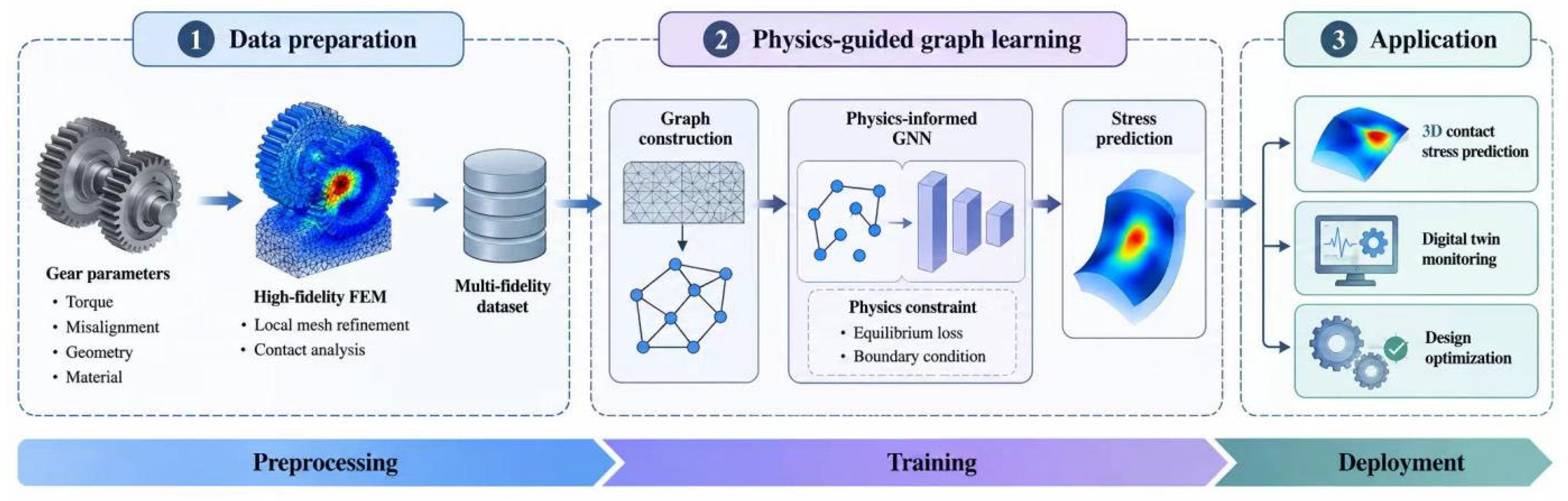
Figure 1. Technical route of the proposed multi-fidelity physics-informed graph neural network framework.
Processes 14 02706 g001
Figure 2. Adaptive mesh-relaxation loop that preserves contact-zone resolution.
Processes 14 02706 g002
Figure 4. Algorithmic workflow for offline data preparation, curriculum-based physics-constrained training, and separated evaluation protocols.
Processes 14 02706 g004
Figure 5. Multi-objective loss convergence with curriculum learning.
Processes 14 02706 g005
Figure 6. Predicted versus ground-truth von Mises stress on the test set.
Processes 14 02706 g006
Table 1. FEM dataset and simulation configuration.
Gear and
Material Setting
ValueLoading and
Contact Setting
ValueMesh and
Dataset Setting
Value
Gear typeSpur/helicalTorque range100–480 N·mFEM cases5000 cases
Module m 2.0–4.5Misalignment range0–0.30°Train: validation: test3500:750:750
Teeth number18–120Contact formulationAugmented LagrangeElement typeSOLID187
Pressure angle20°Friction coefficient0.10Contact-region mesh size0.5 mm
Helix angle0–25°Penetration tolerance<1.0 × 10⁻³ mmFar-field mesh size1.0 mm
Face width18–74 mmContact stiffness1.0 (program-controlled factor)Typical high-fidelity nodes1 × 106
Material grade42CrMo4SolverANSYS 2026 R1 MechanicalTypical coarse graph nodes5 × 105
Young’s modulus206 GPa Hardware96 GB GPU
Poisson’s ratio0.3
Table 2. Neural-network training configuration.
ModuleParameterValue
Network architectureBackboneGated GraphSAGE
Graph layers/hidden channels5/128
Activation/normalizationSiLU/LayerNorm
RegularizationDropout/gradient clippingDropout = 0.1; global gradient norm clipped at 10.0
OptimizationOptimizerAdamW
Learning rate/weight decay1.0 × 10−3/1.0 × 10−5
LR scheduleWarm-up + cosine restarts
TrainingBatch size/epochs1 graph/100
Train: validation: test70%:15%:15%
LossStress scalingsgn(s) ln(1 + |s|/10 MPa), componentwise
Physics/non-contact weightsλphys,max = 0.5; λmask = 0.02
CurriculumPhysics schedule0 for epochs 1–20; ramp 21–29; full 30–100
SamplingPhysics nodes10%, capped at 8192
ReproducibilityPrimary seed/additional full-model seeds42/37, 55, 73, 91
Table 7. Multi-fidelity projection-strategy comparison.
Projection StrategyCoarse-Graph NMSEPeak-Stress ErrorComplementary-Energy Error
Distance-weighted average1.18 × 10−43.1%2.8%
Maximum projection8.87 × 10−52.3%2.1%
Table 3. Ablation study of key architectural and training components (seed 42, unless noted).
VariantChanged ComponentNMSER2Peak-Stress ErrorPeak VRAM
Ours-Full (conditioned)All components; projected stress prior; five-seed mean ± SD(9.1 ± 0.4) × 10−50.985 ± 0.0012.5 ± 0.2%47.6 GB
Ours-GeometryGateStress terms removed from gateNot reportedNot reported4.1% (seed 42)Not reported
Ours-NoGatePhysical edge gate removed1.74 × 10−40.96415.6%46.8 GB
Ours-AutoGradAD equilibrium residual; full-graph OOMNot availableNot availableNot available>100 GB projected; OOM
Ours-WeightedAvgDistance-weighted projection1.18 × 10−40.9783.1%47.3 GB
Ours-NoCurriculumFull physics weight from epoch 11.46 × 10−40.9715.4%47.8 GB
Ours-NoMaskSpatial mask loss removed9.6 × 10−50.9832.5%47.4 GB
Table 4. Internal baseline comparison on the same gear-contact test set.
MethodTraining/Input RepresentationNMSER2Peak-Stress ErrorForward/Solve TimeParametersFLOPs
High-fidelity FEMNative dense FEM meshReference1.000Reference4.5 h0
5-layer GCNCoarse graph, isotropic aggregation3.82 × 10−40.94417.6%35 ms111,5601.28 × 1011
GCN + PriorCoarse graph, isotropic, with prior1.42 × 10−40.9765.8%36 ms112,2001.31 × 1011
GraphSAGECoarse graph, mean aggregation2.61 × 10−40.96114.2%39 ms194,1202.00 × 1011
Point-cloud PINNCoordinate MLP with AD residual1.93 × 10−40.9708.9%210 ms268,5502.69 × 1011
Proposed (conditioned)Multi-fidelity gated graph + LSFD8.7 × 10−50.9852.3%42 ms conditioned pass196,6802.39 × 1011
Table 5. Error distribution across training, validation, and test splits.
SplitCasesNMSER2Median |Error|95th Percentile |Error|Peak-Stress Error
Training35008.2 × 10−50.9873.1 MPa11.4 MPa2.1%
Validation7508.9 × 10−50.9863.3 MPa12.1 MPa2.4%
Test750(9.1 ± 0.4) × 10−50.985 ± 0.0013.5 ± 0.2 MPa12.7 ± 0.5 MPa2.5 ± 0.2%
Table 6. Computational performance and memory profiling across solver frameworks.
Solver FrameworkGradient ComputationHardwarePeak MemoryForward/Solve Time
Traditional FEMAnalytical FEM residual64-core HPC clusterNot reported4.5 h
Standard point-cloud PINNReverse-mode AD96 GB GPU>100 GB projected; OOMNot available
Proposed PINN–GNN (conditioned)Unstructured LSFD96 GB GPU47.6 GB measured42 ms conditioned pass
Disclaimer/Publisher’s Note: The statements, opinions and data contained in all publications are solely those of the individual author(s) and contributor(s) and not of MDPI and/or the editor(s). MDPI and/or the editor(s) disclaim responsibility for any injury to people or property resulting from any ideas, methods, instructions or products referred to in the content.