Hybrid Grey-Box–ARX Identification and Constrained Model Predictive Control of a 250 L Jacketed Batch Milk Pasteurizer

Abstract

This study presents an experimental framework for hybrid grey-box–ARX identification and constrained model predictive control (MPC) in a 250 L jacketed batch milk pasteurizer. The plant was represented as a closed, stirred, energy-accumulating system rather than as a continuous high-temperature short-time process. The workflow combined manufacturer specifications, field measurements, a batch–jacket grey-box model, local autoregressive with exogenous input (ARX) identification in the approach and holding region, and controller evaluation under common sampling, reference, actuator, and exclusion conditions. In five paired experimental blocks, the nominal MPC–ARX reduced RMSE by 1.959 °C, IAE by 7801 °C s, specific energy consumption by 0.0081 kWh/kg, overshoot by 3.573 °C, actuator saturation by 44.46 percentage points, and thermal overexposure by 4717 °C s relative to a fixed-parameter PI controller with anti-windup. The optimization remained feasible at all evaluated instants, with a mean computation time of 6.4 ms for a 5 s control period. Supervised adaptive strategies provided diagnostic value but did not outperform the nominal MPC. The conclusions are restricted to batches near the nominal fill condition and the 65 °C/30 min milk recipe.

1. Introduction

Thermal pasteurization integrates food-safety requirements, product stability, quality preservation, and energy use within a single processing stage. In dairy and other heat-sensitive products, temperature control must therefore regulate not only the nominal setpoint but also exposure time, thermal overshoot, spatial uniformity, and energy demand. Recent research has addressed event-based optimization of food thermal processing [1], energy and exergy performance in milk pasteurization [2], advanced control of continuous-flow ohmic heating [3], adaptive pasteurization control [4], predictive control of extrusion [5], and industrial drying [6]. These applications show the value of incorporating process dynamics and operational constraints, but they represent different thermal architectures and should not be treated as interchangeable evidence.

A jacketed batch pasteurizer differs fundamentally from a continuous high-temperature short-time (HTST) line. The product remains in a stirred sanitary vessel while heat is transferred indirectly through a service jacket; there is no continuous product flow, holding tube, or dominant regenerative section. The controlled temperature therefore represents the thermal state of an accumulated product mass rather than the outlet temperature of a continuous stream. Appropriate models must account for product and jacket thermal capacities, wall and heat-loss effects, agitation, spatial temperature dispersion, actuator limits, and measurement delays. Direct transfer of continuous heat-exchanger or HTST models to this configuration may therefore produce an incorrect representation of the plant dynamics.

Thermal-system modeling increasingly combines physical balances with parameter estimation and operational data. Mechanistic and grey-box representations preserve physical interpretation and energy consistency, whereas lumped and transfer-function models facilitate identification, diagnosis, and controller synthesis [7,8,9,10]. Online estimation, Kalman-filter-based methods, reinforcement learning, fractional-order formulations, and physics-informed models have also been used to represent changing heat-transfer coefficients, uncertainty, and nonlinear thermal behavior [11,12,13,14]. For a jacketed batch system, this supports the use of a batch–jacket grey-box model as a physical plausibility layer, provided that its parameters remain admissible and are validated with data not used for estimation.

PI and PID controllers remain common industrial benchmarks because of their simplicity, low implementation cost, transparency, and operator familiarity [15,16]. However, fixed tuning may lead to delayed correction, overshoot, oscillation, or unnecessary energy use in processes affected by high inertia, delay, saturation, fouling, and changing heat-transfer conditions. Optimized PID, model-free, fractional-order, adaptive, neural-network-based, and uncertainty-compensation strategies have consequently been proposed for thermal systems [17,18,19,20,21,22]. Their adoption in food processing nevertheless requires more than improved tracking: actuator feasibility, thermal constraints, holding-time traceability, and operational stability must also be preserved.

Model predictive control (MPC) is attractive for jacketed batch pasteurization because it can anticipate thermal evolution, penalize abrupt input changes, and enforce power and temperature constraints. Its performance depends on prediction and control horizons, cost-function weights, constraint formulation, and solver feasibility [23,24,25,26,27,28,29]. Autoregressive models with exogenous input (ARX) provide a compact discrete representation for this purpose because they relate current temperature to delayed inputs and past outputs. Robust, adaptive, predictive, and state-dependent ARX formulations have been reported for nonlinear or time-varying systems [30,31,32,33].

Previous pasteurization studies provide important foundations but address different process configurations. Khadir and Ringwood developed a first-principles control-oriented representation of an industrial pasteurizer assembled from plate and brazed heat exchangers [34]. Ibarrola et al. studied predictive control of a continuous HTST process [35], while Niamsuwan et al. evaluated multivariable MPC for milk pasteurization through simulation [36]. Experimental comparisons of PID, MPC, and adaptive MPC have also been reported for continuous-flow ohmic heating [3], with related predictive-control applications in extrusion [5] and drying [6]. These systems involve continuous transport, outlet-temperature dynamics, direct volumetric heating, or multistate flow behavior and do not directly reproduce the energy accumulation, indirect jacket transfer, agitation, spatial temperature dispersion, and batch-level replication of a closed jacketed pasteurizer.

This study develops and experimentally evaluates a traceable hybrid grey-box–ARX identification and control framework for a 250 L jacketed batch milk pasteurizer. The framework combines a batch–jacket grey-box model for physical and energy interpretation with a local ARX predictor identified in the approach and holding region. A fixed-parameter PI controller with anti-windup is compared with a nominal constrained MPC under common sampling, reference, actuator, and exclusion conditions, while supervised ARX observation, PI retuning, and adaptive MPC are evaluated separately as diagnostic, secondary, and exploratory extensions.

The contribution is methodological and experimental rather than algorithmic. The study integrates measured active electrical power, three-sensor spatial temperature supervision, formal acceptance and rejection criteria for adaptive updates, independent model-validation records, and batch-level paired controller comparisons. This design allows tracking, energy consumption, actuator saturation, feasibility, and thermal overexposure to be evaluated within a unified workflow. The conclusions are restricted to the experimentally represented operating domain and do not imply universal MPC superiority, microbiological validation, or sanitary certification.

2. Theoretical Background

2.1. Jacketed Batch Pasteurization as a Controlled Thermal Process

Thermal pasteurization links food safety, product stability, quality preservation, and energy consumption within a single dairy-processing stage [2,37,38]. From a control perspective, reaching the nominal setpoint is insufficient: the controller must also limit overshoot, avoid insufficient thermal treatment, maintain the required holding condition, reduce unnecessary heating, and operate within actuator and safety constraints. These requirements have been addressed directly in pasteurization control [4,35,36] and, in related food thermal processes, through event-based optimization [1], continuous-flow ohmic heating [3], extrusion [5], and drying [6].

The evaluated jacketed batch pasteurizer differs fundamentally from continuous high-temperature short-time (HTST) systems, in which product flow, residence time, regeneration, heating, holding, and cooling are coupled [39,40,41]. Here, milk remains in a stirred vessel and receives heat indirectly through a service jacket; consequently, the controlled temperature represents an accumulated product mass rather than the outlet of a continuous stream.

This architecture requires consideration of energy accumulation, batch–jacket and wall heat transfer, mixing and spatial dispersion, actuator limits, and sensor delay. Continuous heat-exchanger or HTST models therefore require reformulation. Accordingly, the complete batch was the experimental unit, while time samples were used only for identification, prediction, controller execution, and performance calculation.

Thermal overexposure was also distinguished from microbiological lethality. The former is a linear degree–time indicator of controller-induced thermal excess, whereas equivalent lethality $F(T_{\mathrm{r}\mathrm{e}\mathrm{f}},z)$ exponentially weights the complete temperature trajectory using target-specific kinetics. The conventional $F_0$ value, defined at 121.1 °C with $z=10$ °C, is a sterilization metric and not the appropriate primary criterion for the evaluated 65 °C pasteurization treatment. A microbiologically meaningful pasteurization value requires validated D- and z-values for the relevant microorganism–matrix combination [42,43].

2.2. Hybrid Grey-Box–ARX Identification for Thermal Systems

Model-based control depends on whether the selected representation is appropriate for prediction, optimization, and controller design [16,44,45]. First-principles models based on mass and energy balances preserve physical interpretability and help to verify consistency with the plant configuration [34,41]. However, detailed modeling of jacketed food-processing equipment is limited by uncertainty in heat-transfer coefficients, jacket dynamics, wall thermal capacity, product properties, mixing, heat losses, and sensor delays.

Data-driven system identification provides a complementary representation by estimating dynamic relationships directly from experimental input–output records [44]. It can capture plant-specific behavior such as actuator saturation, sensor response, local losses, and operating constraints, but a purely empirical model may reproduce short-term behavior without preserving physical or energy consistency.

The hybrid grey-box–ARX framework provides a practical compromise. The batch–jacket grey-box model preserves the process energy structure and supplies physically meaningful bounds, whereas the ARX predictor provides a compact discrete representation for short-horizon control in the approach and holding region. This combination is consistent with work on heat-exchanger modeling and monitoring [7,8,10], experimental parameter estimation [12], mechanism-supported thermal modeling [14], and compact ARX-based predictive structures [30,31,32,33].

The objective is not to reproduce the complete batch cycle through a high-fidelity simulator. Instead, the grey-box model acts as a physical and energy plausibility layer, while the ARX predictor supports local prediction and real-time constrained MPC. Throughout this manuscript, “batch–jacket grey-box model” refers to the physical two-state representation, whereas “hybrid grey-box–ARX framework” refers to the combined use of this model and the local ARX predictor.

2.3. PI/PID Controllers as Industrial Benchmarks

PI and PID controllers remain standard benchmarks for industrial thermal systems because they are simple, transparent, widely available in automation platforms, and familiar to plant operators [15,16]. In jacketed batch pasteurization, they regulate the mean product temperature by manipulating electrical heating power or an equivalent thermal input. They therefore provide an appropriate conventional baseline for determining whether predictive control yields a practically meaningful improvement.

Fixed-parameter feedback is nevertheless reactive. In systems affected by high thermal inertia, indirect heating, actuator saturation, sensor delay, fouling, or changing heat-transfer conditions, fixed tuning may lead to delayed correction, overshoot, oscillation, prolonged settling, or unnecessary energy use. Fouling and heat-transfer degradation can also modify process gain, delay, and dominant time constants [46,47,48].

Alternative approaches include optimized PID and model-free control [18,22], fractional-order control [20], adaptive and neural-network-based tuning [17,19], and predictive thermal control [21]. Their use in food processing must be assessed beyond tracking accuracy because actuator activity, thermal constraints, holding-time traceability, and operational stability must also be preserved. Accordingly, this study uses a fixed-parameter PI controller with anti-windup as the conventional benchmark under the same reference, sampling, actuator, and exclusion conditions applied to MPC.

2.4. Constrained Model Predictive Control for Energy-Aware Thermal Regulation

Model predictive control uses a dynamic model to forecast process outputs over a finite horizon and determines the control action by solving an optimization problem at each sampling instant [40,45]. For jacketed batch pasteurization, MPC is attractive because it can anticipate temperature evolution, limit abrupt changes in heating power, enforce actuator constraints, and penalize trajectories associated with excessive thermal exposure.

Predictive control has been studied directly for industrial and milk pasteurization systems [34,35,36]. Related experimental and industrial applications include continuous-flow ohmic heating [3], extrusion [5], drying [6], and heat-exchanger control [25,29]. More broadly, MPC studies show that horizon selection, penalty weights, constraint formulation, and computational feasibility directly affect tracking and energy performance [23,24,26,27,28].

In this study, constrained MPC uses the nominal ARX predictor identified in the approach and holding region. The ARX model provides short-horizon predictions, whereas the batch–jacket grey-box model retains the plant’s physical and energy interpretation. This division favors feasibility, traceability, and real-time implementation over a more complex black-box strategy.

The expected advantage over the fixed-parameter PI controller is not limited to lower setpoint error. Anticipating the thermal trajectory may also reduce overshoot, actuator saturation, unnecessary energy use, and thermal overexposure. Controller performance was therefore evaluated using tracking error, accumulated error, actuator activity, saturation, specific energy consumption, valid holding time, optimization feasibility, and computation time.

2.5. Supervised Adaptation and Operational Hypotheses

Supervised adaptation may be useful when thermal dynamics vary because of drift, product variability, sensor behavior, fouling, or heat-transfer degradation. Adaptive control has been studied directly in pasteurization [4] and in related thermal systems using mechanism-supported estimation and adaptive tuning [14,17,19]. However, online updates may become unreliable under insufficient excitation, actuator saturation, invalid measurements, mode transitions, or physically inadmissible parameter estimates.

Broader robust adaptive frameworks address time-varying uncertainty and unmodeled nonlinear dynamics. Liu et al. [49] proposed a hierarchical adaptive formation-tracking method that separates exosystem estimation from the control layer and applies the congelation-of-variables principle to establish boundedness and convergence. Liu et al. [50] developed a congealed neural-network architecture that decomposes time-varying uncertainty into an adaptively estimated component and a nonlinear residual, with an additional robust term to attenuate approximation bias. These approaches illustrate how hierarchical estimation and residual approximation can extend fixed-dimensional linear adaptation. However, they were developed for networked or spatiotemporal nonlinear systems and are not directly transferable to the lumped single-unit pasteurizer. They therefore motivate future extensions rather than validate the present ARX–RLS design.

Accordingly, adaptation was treated as a supervised extension rather than an automatic replacement for nominal MPC. C1 operated as an observation-only ARX–RLS layer that screened candidate updates before they could affect C2 or C4, thereby separating controller improvement from effects caused by re-identification or retuning.

Five operational hypotheses were evaluated:

H1. 

The hybrid grey-box–ARX framework combines physical consistency, parsimony, and local predictive capacity.

H2. 

Nominal constrained MPC–ARX reduces tracking error relative to fixed-parameter PI control without compromising holding conditions, actuator constraints, feasibility, or real-time execution.

H3. 

Supervised adaptation improves performance under slow drift only when updates are sufficiently excited, stable, physically admissible, and diagnostically justified.

H4. 

Constrained MPC or supervised adaptation reduces specific energy consumption or thermal overexposure while preserving non-inferior tracking.

H5. 

Adaptive MPC improves multihorizon prediction only when its predictive benefit outweighs any increase in energy use or actuator activity.

3. Materials and Methods

The methodology was developed for a 250 L jacketed batch milk pasteurizer treated as a closed, stirred, energy-accumulating system rather than as a continuous high-temperature short-time (HTST) line. During heating and holding, the plant had no continuous product flow, holding tube, or dominant regenerative section. The workflow combined plant specifications, a batch–jacket grey-box model, and a local ARX predictor for short-horizon control. Fixed PI control, supervised adaptive extensions, and constrained MPC–ARX were evaluated under common sampling, reference, actuator, and exclusion conditions.

Manufacturer and design specifications defined the physical domain, model initialization, plausibility bounds, and operating constraints. Experimental measurements were used for parameter estimation, independent validation, controller comparison, and energy-performance calculation. Thus, specifications established admissible limits, whereas the reported results were derived from measured experimental batches.

3.1. Experimental Design and Comparative Architecture

The complete batch was the experimental unit. Time samples supported identification, prediction, controller execution, and indicator calculation but were not treated as independent statistical replications. The primary confirmatory comparison was C3–C0: nominal constrained MPC based on the fixed ARX model versus fixed-parameter PI control with anti-windup. C1 was an observation-only adaptive ARX layer, C2 was evaluated secondarily against C0, and C4 was evaluated exploratorily against C3.

All strategies used the same control period, actuator limits, reference trajectory, enabled sensors, initial-condition criteria, and scenario definitions. C4 was kept separate from the C3–C0 comparison to preserve the confirmatory role of the nominal MPC.

The C3–C0 contrast was a practical industrial benchmark, not a complexity-matched controller comparison. C0 included anti-windup, actuator saturation, input-rate limitation, and bumpless transfer; its tuning was fixed after the pilot stage. The comparison therefore quantified the incremental benefit of prediction and explicit constraint handling relative to this conventional baseline, but not superiority over gain-scheduled PI, nonlinear PID, adaptive control, nonlinear MPC, or other advanced strategies.

Table 1. Controller architecture and comparative role.

Code	Strategy	Associated Model	Comparative Role	Main Evidence
C0	Fixed-parameter PI controller with anti-windup	Reduced grey-box/ARX support for tuning and interpretation	Conventional benchmark and fallback strategy	RMSE, IAE, overshoot, saturation, actuator activity, valid holding time
C1	Adaptive ARX observer	$M_{ARX,k}$	Separates online identification from improvement in control performance	Predictive error, accepted/rejected updates, parameter stability
C2	Supervised self-tuning PI controller	$M_{ARX,k}$	Secondary comparison under slow drift	RMSE, IAE, saturation, energy use, admissible parameter update
C3	Nominal constrained MPC-ARX	Fixed $M_{ARX}$	Primary predictive comparison against C0	RMSE, IAE, specific energy consumption, overshoot, saturation, feasibility, computation time
C4	Adaptive MPC-ARX	$M_{ARX,k}$	Exploratory extension under reproducible drift	Multihorizon prediction error, feasibility, computation time, fallback activations

summarizes the controller architecture, associated model, comparative role, and main evidence used in the study.

3.2. Experimental Plant and Operating Domain

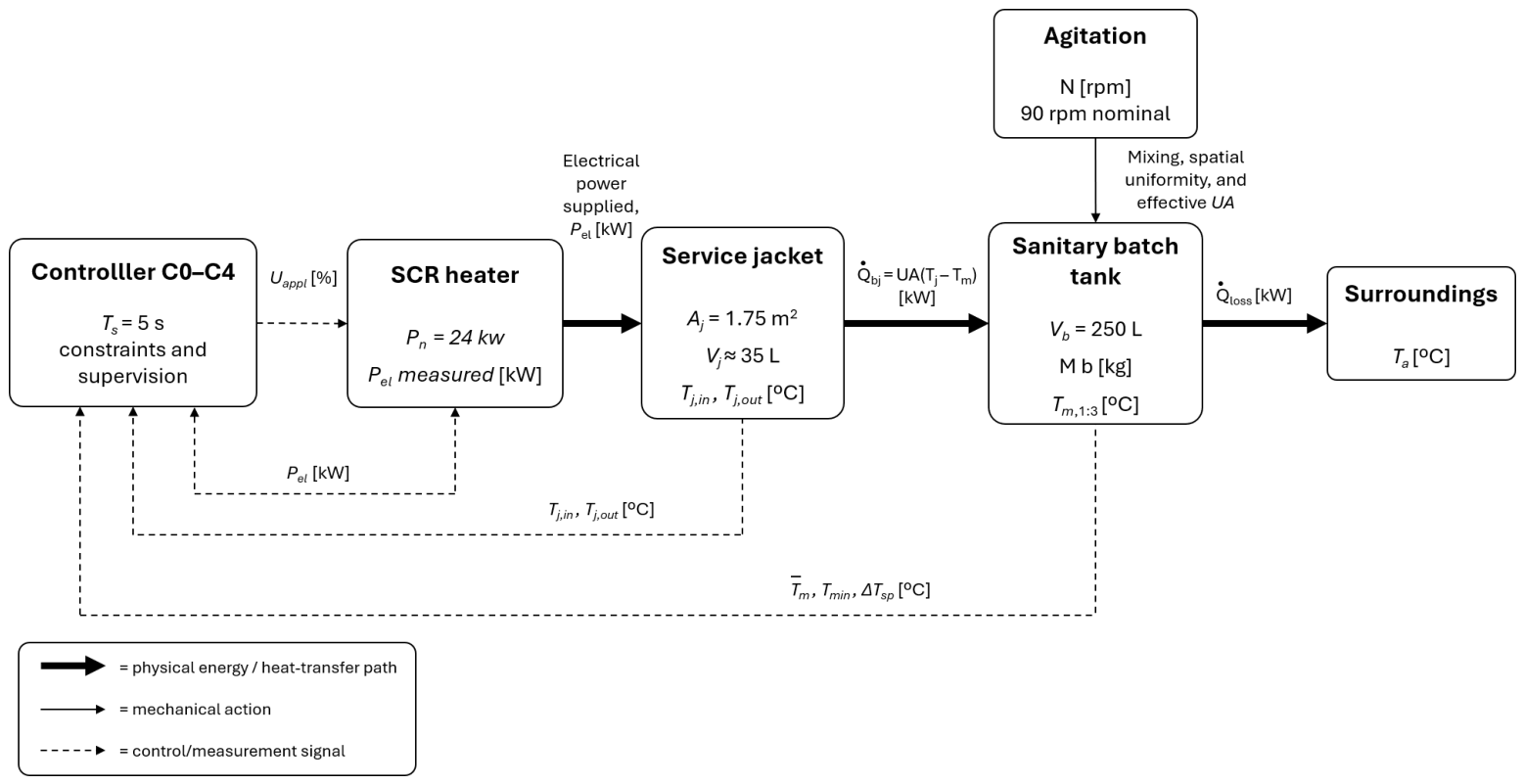
The experimental plant was a sanitary jacketed batch pasteurizer with a gross capacity of 300 L and a useful capacity of 250 L. It comprised an external service jacket, indirect electrical heating, service-fluid recirculation, and mechanical agitation. As shown in Figure 1, the applied command drove the SCR heater, active electrical power was measured at the heater input, and heat was transferred through the service jacket to the accumulated product mass. Agitation influenced mixing, spatial temperature dispersion, and effective batch–jacket heat transfer. Product-temperature, jacket-temperature, and active-power measurements were returned to the controller and supervisory system. This architecture defined the boundaries of the batch–jacket grey-box model, ARX predictor, and MPC formulation.

Table 2. Plant parameters used for modeling, identification, and control.

Quantity	Reference Value	Status	Methodological Use
Useful/gross capacity	250 L/300 L	Manufacturer specification	Defines nominal batch capacity, headspace, and equipment geometry
Permissible fill range	150–250 L	Equipment operating specification; not fully validated experimentally	Defines equipment limits and future fill-level robustness scenarios
Thermal recipe	65 °C setpoint; 30 min holding; 63 °C threshold	Experimental protocol	Defines the regulation target and operational holding criterion
Service jacket	$A_j=1.75 {\mathrm{m}}^2$; $V_j\approx 35 \mathrm{L}$	Design values	Supports jacket-capacity and conductance calculations
Heating system	24 kW electrical heater with SCR actuation	Verified and monitored	Defines the actuator limit and measured input for energy calculations
Hot/cold service flow	3.0/4.0 ${\mathrm{m}}^3/\mathrm{h}$	Monitored when available	Characterizes service-side disturbances and heat-transfer conditions
Cold service	0–2 °C; 20–25 kW	Equipment reference	Defines the cooling mode, which was excluded from the heating ARX model
Agitation	90 rpm nominal; 60–120 rpm permissible range	Nominal operating condition and equipment specification	Supports mixing, spatial uniformity, and heat-transfer interpretation
Instrumentation	Three product Pt100 sensors; two jacket Pt100 sensors; power, flow, and VFD signals	Experimental setup	Provides control outputs, supervision variables, disturbances, and energy data
Acquisition and control	1–2 s raw acquisition; 5 s control period	Fixed	Defines causal resampling and execution of ARX, RLS, PI, and MPC algorithms
Initial thermal parameters	$C_m\approx 1.04 \mathrm{M}\mathrm{J}/\mathrm{K}$; ${\Gamma }_0\approx 790 \mathrm{W}/\mathrm{K}$	Initial grey-box values	Supports model initialization and heating-time plausibility assessment

summarizes the plant specifications and operating conditions used for modeling, identification, and control.

The permissible 150–250 L fill range was not fully represented experimentally; the analyzed batches were concentrated near the nominal 250 L condition. The study therefore evaluates batch-to-batch variability near nominal fill rather than robustness across the complete equipment range.

The batch cycle comprised loading, mixing, rapid heating, approach, holding, cooling, and discharge. ARX identification and the C3–C0 evaluation were restricted to the approach and holding region, where a local predictor was considered appropriate. Rapid-heating data supported energy-balance and effective-capacity assessment, whereas cooling was treated separately because its service conditions and heat-flow direction differed from heating and holding.

All confirmatory experiments used milk and the same recipe: a 65 °C setpoint, 30 min holding period, and 63 °C minimum operational threshold. The observed batch mass, initial temperature, and agitation ranges were 242.57–270.42 kg, 17.53–24.46 °C, and 60–120 rpm, respectively. These ranges define the empirical domain; the complete fill range, alternative recipes, and other dairy formulations were not experimentally validated.

3.3. Signals, Instrumentation, and Data Acquisition

The controlled output was the mean batch temperature calculated from three valid product sensors:

$$y\left(k\right)=T_{m,avg}\left(k\right)={\displaystyle \frac{1}{N_T}}{\displaystyle \sum _{i=1}^{N_T}}{T}_{m,i}\left(k\right), N_T=3$$

(1)

Independent supervision used the minimum product temperature and the spatial temperature dispersion:

$$T_{m,min}\left(k\right)=\underset{i}{min}{T}_{m,i}\left(k\right), \Delta T_m\left(k\right)=\underset{i}{max}{T}_{m,i}\left(k\right)-\underset{i}{min}{T}_{m,i}\left(k\right)$$

(2)

Valid holding time was accumulated only when all sensors remained valid, the minimum product temperature exceeded the required threshold, and the spatial dispersion remained within the admissible tolerance:

$$t_{hold,val}=T_s\sum _{k\in K_{hold}}\mathbf{1}\left[T_{m,min}\left(k\right)\ge T_{req}\wedge \Delta T_m\left(k\right)\le \Delta T_{adm}\right]$$

(3)

This criterion was used as an operational engineering indicator of time–temperature compliance. It was not interpreted as microbiological validation or sanitary certification.

The manipulated input was the normalized heating command $u\left(k\right)\in \left[0,1\right]$. However, energy calculation and energy identification were based on measured active electrical power. The command-to-thermal-power relationship was retained only as an auxiliary model:

$$P_{th}\left(k\right)={\eta }_{th}\left(k\right)P_{N}u\left(k\right), 0<{\eta }_{th}\left(k\right)\le 1$$

(4)

Raw data were acquired using a common time reference at 1–2 s. Control execution, ARX prediction, RLS updating, and MPC optimization were performed at $T_s=5$ s after causal resampling.

Table 3. Measured and derived variables and their methodological function.

Signal	Unit	Source	Use in the Study
$T_{m,1:3}$	°C	Product Pt100 sensors	Calculation of $y$, $T_{m,min}$, $\Delta T_m$, holding validation, and mixing diagnosis
$T_{j,i}$, $T_{j,o}$	°C	Jacket inlet/outlet sensors	Estimation of jacket temperature, service balance, and measured disturbance
$P_{el}$, $E_{el}$	kW, kWh	Electrical power analyzer	Physical input, specific energy consumption, and energy-balance check
$u_c$, $u$	-	Controller/supervisor	Computed command and applied command after saturation, ramp limits, and interlocks
${\dot{V}}_j$, $N$, $T_a$, $m_b$	${\mathrm{m}}^3/\mathrm{h}$, rpm, °C, kg	Flow meter, VFD, ambient sensor, weighing	Disturbances, blocking factors, and effective-capacity calculations
Status and alarms	Code	PLC/supervisor	Segmentation, exclusion criteria, safety, and traceability

summarizes the critical measured and derived signals.

Data were partitioned by batch and by block into estimation, selection, validation, and comparison subsets. Records used to tune or select models were not used as confirmatory evidence. Samples with quality flags were retained in the raw database but excluded from the affected mathematical window.

3.4. Batch–Jacket Grey-Box Model

The plant was represented by a two-state batch–jacket grey-box model describing energy accumulation in the product and effective jacket dynamics. Additional states were omitted because they were not reliably identifiable with the available sensors. The model supported parameter initialization and bounding, physical interpretation of the ARX predictor, and energy-consistency assessment.

The state vector, jacket-temperature approximation, and output were defined as

$$x\left(t\right)=\left[\begin{array}{c}{T}_m\left(t\right)\\ T_j\left(t\right)\end{array}\right]$$

(5a)

$$T_j\left(t\right)\approx {\displaystyle \frac{T_{j,i}\left(t\right)+T_{j,o}\left(t\right)}{2}}$$

(5b)

$$y\left(t\right)=T_{m,avg}\left(t\right)$$

(5c)

The effective thermal capacities were written as

$$C_m=m_b{c}_{p,m}+C_{met,m}$$

(6a)

$$C_j={\rho }_j{V}_{j,ef}{c}_{p,j}+C_{met,j}$$

(6b)

The batch–jacket grey-box model conductance was represented as

$$\Gamma \left(N,R_f\right)=U_{ef}\left(N,R_f\right)A_{j,ef}$$

(7a)

$${\displaystyle \frac{1}{U_{ef}}}={\displaystyle \frac{1}{h_m\left(N\right)}}+{R^{\prime }}_f+{\displaystyle \frac{{\delta }_w}{k_w}}+{\displaystyle \frac{1}{h_j}}$$

(7b)

Because the individual thermal resistances were not separately identifiable from the available measurements, $\Gamma$ was estimated as an aggregated parameter.

During heating and holding, the energy balances were

$$C_m{\dot{T}}_m=\Gamma \left(T_j-T_m\right)-H_m\left(T_m-T_a\right)$$

(8)

$$C_j{\dot{T}}_j={\eta }_h{P}_{el}\left(t\right)-\Gamma \left(T_j-T_m\right)-H_j\left(T_j-T_a\right)$$

(9)

The local linear form around an operating condition was

$$\dot{x}\left(t\right)=A_{c}x\left(t\right)+B_p{P}_{el}\left(t\right)+B_a{T}_a\left(t\right)$$

(10)

with matrices derived from $C_m$, $C_j$, $\Gamma$, $H_m$, and $H_j$. First-order discretization or zero-order-hold discretization linked the physical model to the ARX representation:

$$x_{k+1}=A_d{x}_k+B_d{P}_{el}\left(k\right)+E_d{T}_a\left(k\right), y_k=C_d{x}_k+v_k$$

(11)

Energy consistency was evaluated over each moving window using

$${ϵ}_E={\displaystyle \frac{\left|E_{el}-\Delta U_m-\Delta U_j-E_{loss}\right|}{\mathrm{m}\mathrm{a}\mathrm{x}\left(E_{el},\left|\Delta U_m+\Delta U_j\right|,{ϵ}_0\right)}}$$

(12)

Persistently high ${ϵ}_E$ values were interpreted as indicators of power-measurement problems, omitted losses, incorrect effective thermal mass, or operation outside the model validity domain.

3.5. ARX Identification and Discrete-Model Validation

The ARX model was formulated in deviation variables as a local predictor for the approach and holding region:

$$\tilde{y}\left(k\right)=y\left(k\right)-y_0, \tilde{u}\left(k\right)=u\left(k\right)-u_0, {\tilde{d}}_j\left(k\right)=d_j\left(k\right)-d_{j,0}$$

(13)

The candidate structure was

$$A\left(q^{-1}\right)\tilde{y}\left(k\right)=B_u\left(q^{-1}\right)q^{-n_{k,u}}\tilde{u}\left(k\right)+{\displaystyle \sum _{j=1}^{n_d}}{B}_{d,j}\left(q^{-1}\right)q^{-n_{k,j}}{\tilde{d}}_j\left(k\right)+e\left(k\right)$$

(14)

with

$$A\left(q^{-1}\right)=1+a_1{q}^{-1}+\cdots +a_{n_a}{q}^{-n_a}$$

(15a)

$$B_u\left(q^{-1}\right)=b_1{q}^{-1}+\cdots +b_{n_b}{q}^{-n_b}$$

(15b)

For $T_s=5$ s, the candidate set comprised $n_a\in \{2,3,4\}$, $n_b\in \{2,3,4\}$, and $n_{k,u}\in \{1,2,3\}$. Candidate inputs were the normalized command $u\left(k\right)$ and measured active electrical power $P_{\mathrm{e}\mathrm{l}}\left(k\right)$. The latter was preferred because it represented the energy supplied to the process more directly, but it was used only when continuous, synchronized, and sufficiently excited. Otherwise, $u\left(k\right)$ served as an auxiliary input, and the choice was recorded for traceability.

The parameter vector was estimated using

$$Y=\Phi \theta +e, \widehat{\theta }={\left({\Phi }^T\Phi \right)}^{-1}{\Phi }^{T}Y$$

(16)

Weighted least squares was used when uncertainty varied across windows. Model selection combined out-of-sample performance, parsimony, discrete-time stability, multi-step and free-simulation errors, and residual autocorrelation. The response was also required to preserve a physically consistent gain sign and energy behavior. A near-unit pole was retained when it represented actual batch-energy accumulation. The nominal ARX model was fixed before controller tuning and comparative evaluation.

Model mismatch was defined as the difference between the response predicted by the fixed nominal ARX model and the measured plant response under conditions differing from those represented during identification. Anticipated sources included variations in effective thermal capacity, batch–jacket conductance, heat losses, mixing, product properties, actuator gain, sensor dynamics, effective input delay, and unmeasured disturbances. Batch-mass changes alter thermal capacity and the dominant heating dynamics, whereas recipe or composition changes may affect heat capacity, viscosity, mixing, fouling, heat transfer, and the local operating point.

Mismatch was assessed through independent one-step, multihorizon, and free-simulation errors; gain sign and stability; energy closure; and the prediction-error diagnostics of the supervised ARX–RLS observer. These criteria evaluated local adequacy for short-horizon control and were not interpreted as evidence that the same coefficients remained valid for untested batch sizes, products, or recipes.

The conservation structure can be retained for similar closed, stirred, indirectly heated jacketed vessels, but its numerical parameters are plant specific. Transfer to such equipment requires recalibration of thermal capacities, conductance, heat losses, actuator efficiency, and measurement dynamics, together with ARX re-identification. Capacity changes require reparameterization rather than proportional volume scaling because thermal mass, heat-transfer area, service circulation, and surface-to-volume ratio do not scale uniformly. Processes involving direct steam injection, spray or immersion heating, rotation, pressure-dependent operation, or continuous transport require additional balance terms and partial or complete model reconstruction.

3.6. Supervised Adaptation and Controllers

Supervised recursive least squares (RLS) was used for adaptive parameter estimation. For a regressor $\varphi \left(k\right)$, the update equations were

$$K\left(k\right)={\displaystyle \frac{P\left(k-1\right)\varphi \left(k\right)}{\lambda +{\varphi }^T\left(k\right)P\left(k-1\right)\varphi \left(k\right)}}$$

(17)

$$\widehat{\theta }\left(k\right)={\Pi }_{{\Omega }_{\theta }}\left\{\widehat{\theta }\left(k-1\right)+K\left(k\right)\left[y\left(k\right)-{\varphi }^T\left(k\right)\widehat{\theta }\left(k-1\right)\right]\right\}$$

(18)

$$P\left(k\right)={\lambda }^{-1}\left[I-K\left(k\right){\varphi }^T\left(k\right)\right]P\left(k-1\right), 0<\lambda \le 1$$

(19)

Raw RLS candidates were not incorporated automatically into the observer or controller. Each update passed through a sequential gate comprising data eligibility, excitation sufficiency, and model admissibility. All thresholds were calibrated from pilot-stage records and fixed before the comparative campaign.

For excitation diagnosis, regressors were normalized using pilot-stage scaling factors. Over a moving window of $N_w$ samples, the normalized information matrix was calculated as

$$R_{\phi ,k}={\displaystyle \frac{1}{N_w}}{\displaystyle \sum _{i=k-N_w+1}^k}{\overline{\phi }}_i{\overline{\phi }}_i^{\mathrm{T}}$$

The window was considered sufficiently informative only when

$${\lambda }_{\mathrm{m}\mathrm{i}\mathrm{n}}\left(R_{\phi ,k}\right)\ge {\epsilon }_{\mathrm{P}\mathrm{E}}\mathrm{and}\kappa \left(R_{\phi ,k}\right)\le {\kappa }_{\mathrm{m}\mathrm{a}\mathrm{x}}$$

where ${\lambda }_{\mathrm{m}\mathrm{i}\mathrm{n}}$ and $\kappa$ denote the minimum eigenvalue and condition number, respectively. These conditions prevented updates under weak excitation or ill-conditioned regressors.

Candidate updates were evaluated only in the approach or holding region, with valid and synchronized temperature and power signals, no active alarm or mode transition, no persistent actuator saturation, acceptable spatial temperature dispersion, and energy-closure error below its prescribed limit. Failure of any eligibility or excitation condition froze adaptation and retained the previous validated parameters.

Eligible candidates were then required to preserve a positive and bounded static gain, satisfy the predefined discrete-time stability margin and parameter bounds, and avoid abrupt parameter changes. Parameter continuity was evaluated using

$$d_{\theta ,k}^2={\left({\widehat{\theta }}_k^{\hspace{0.17em}c}−{\widehat{\theta }}_{k-1}\right)}^{\mathrm{T}}{P}_{k-1}^{-1}\left({\widehat{\theta }}_k^{\hspace{0.17em}c}−{\widehat{\theta }}_{k-1}\right)$$

where ${\widehat{\theta }}_k^{\hspace{0.17em}c}$ is the raw candidate vector. For the four-parameter ARX structure, the candidate was required to satisfy

$$d_{\theta ,k}^2\le {\chi }_{4,0.99}^2=13.28$$

An update was accepted only when all eligibility, excitation, conditioning, stability, gain, parameter-continuity, spatial-consistency, actuator, and energy-consistency criteria were satisfied. Otherwise, the candidate was rejected, the previous validated model was retained, and controller retuning or adaptive-MPC model replacement was not authorized.

Table 4. Diagnostic framework for accepting or rejecting supervised ARX–RLS updates.

Diagnostic Level	Criterion	Diagnostic Quantity	Threshold Used in the Study	Action if Criterion Fails
Operating domain	Valid process mode	Process-mode flag	Approach or holding mode only	Freeze adaptation and retain the previous validated model
Signal validity	Required measurements available	Product-temperature sensors, active-power signal, timestamps, and alarm flags	All required signals valid and synchronized; no active alarm	Reject the candidate update
Spatial consistency	Acceptable product-temperature dispersion	ΔTsp	ΔTm ≤ 0.50 °C	Reject the candidate update and retain the previous parameters
Actuator condition	Absence of persistent saturation	|ucalc − uappl| and number of consecutive samples at an actuator limit	|ucalc − uappl| ≤ 0.060 p.u. and fewer than 12 consecutive saturated samples (60 s)	Freeze adaptation until the actuator returns to the admissible region
Excitation	Minimum regressor information	λmin(Rφ,k)	λmin(Rphi,k) ≥ εPE = 1.0 × 10−4 (Nw = 60; 300 s)	Reject the update because of insufficient excitation
Numerical conditioning	Acceptable regressor conditioning	κ(Rφ,k)	κ(Rphi,k) ≤ κmax = 1.0 × 104	Reject the update because of ill conditioning
Energy consistency	Acceptable grey-box energy-closure error	εE	|εE| ≤ εE,max = 0.300	Reject the update as outside the energy-validity domain
Dynamic stability	Prescribed discrete-time stability margin	ρmax = maxi |pi|	ρmax ≤ ρlim = 0.99560, with ρlim < 1	Reject the candidate model
Physical gain	Positive and physically admissible static gain	KARX	Kmin ≤ KARX ≤ Kmax, with Kmin > 0	Reject the physically inconsistent model
Parameter continuity	Bounded normalized parameter change	d2θ,k	d2θ,k ≤ 13.28	Reject the abrupt parameter change
Final authorization	All diagnostic gates satisfied	Logical conjunction of all diagnostic flags	All criteria must be satisfied simultaneously	Accept the update; otherwise retain the previous validated model

Note: Regressor scaling, $N_w$, ${\epsilon }_{\mathrm{P}\mathrm{E}}$, ${\kappa }_{\mathrm{m}\mathrm{a}\mathrm{x}}$, ${\epsilon }_{E,\mathrm{m}\mathrm{a}\mathrm{x}}$, ${\rho }_{\mathrm{l}\mathrm{i}\mathrm{m}}$, gain bounds, spatial-dispersion limit, actuator tolerance, and persistent-saturation duration were calibrated during the pilot stage and fixed before the comparative campaign. Accepted updates were considered numerically stable and physically admissible, but not necessarily superior to the nominal ARX model.

summarizes the complete diagnostic sequence, including the criteria, fixed thresholds, and action taken when each condition failed. Acceptance indicated numerical stability and physical admissibility, not predictive or closed-loop superiority. C1 therefore stored accepted updates in observation mode, whereas C2 and C4 could use only models that passed the complete diagnostic gate and the corresponding controller-level authorization. The fixed nominal model and controller remained available as fallback configurations.

The diagnostic gate was designed as a safety and model-admissibility filter rather than as a closed-loop performance selector. RLS minimized local one-step prediction error, whereas controller performance depended on multihorizon prediction, the MPC objective, tracking, specific energy consumption, actuator variation, and thermal overexposure. An accepted model could therefore satisfy all numerical and physical criteria yet remain inferior to the nominal predictor for receding-horizon control. Admissibility alone did not authorize model replacement, and the nominal model remained the fallback configuration.

C0 was the conventional fixed-parameter PI comparator, including saturation, input-rate limitation, bumpless transfer, and anti-windup. In incremental form,

$$u_c\left(k\right)=u_c\left(k-1\right)+K_p\left[e\left(k\right)-e\left(k-1\right)\right]+K_i{T}_{s}e\left(k\right)$$

(20a)

$$u\left(k\right)={\mathrm{s}\mathrm{a}\mathrm{t}}_{\left[u_{min},u_{max}\right]}\left\{u_c\left(k\right)\right\}$$

(20b)

C1 updated the ARX model in observation mode without affecting the control signal. C2 retuned the PI controller only after complete diagnostic and controller-level authorization. C3 used the fixed nominal ARX model in constrained MPC, whereas C4 used an authorized adaptive model $M_{\mathrm{A}\mathrm{R}\mathrm{X},k}$ as an exploratory extension. This separation prevented improvements caused by re-identification or additional information from being attributed solely to the control law.

The MPC prediction was written as

$${\widehat{Y}}_p\left(k\right)=F{x}_{ARX}\left(k\right)+G\Delta U\left(k\right)$$

(21)

and the optimization problem as

$$\underset{\Delta U}{\mathrm{m}\mathrm{i}\mathrm{n}}J={\displaystyle \sum _{i=1}^{N_p}}{q}_i{\left[\widehat{y}\left(k+i\mid k\right)-r\left(k+i\right)\right]}^2+{\displaystyle \sum _{i=0}^{N_c-1}}{\rho }_i\Delta u^2\left(k+i\right)+{\rho }_{\xi }{\xi }^2$$

(22)

subject to

$$u_{min}\le u\left(k+i\right)\le u_{max}$$

(23a)

$$\Delta u_{min}\le \Delta u\left(k+i\right)\le \Delta u_{max}$$

(23b)

$$y_{min}-\xi \le \widehat{y}\left(k+i\mid k\right)\le y_{max}+\xi$$

(23c)

Prediction horizons, control horizons, weights, constraints, scaling, and solver configuration were adjusted during the pilot stage and fixed before the confirmatory comparison.

3.7. Robustness Assessment of the Nominal Constrained MPC

The assessment examined whether C3 remained operationally adequate under model–plant mismatch. Because C3 was a nominal constrained MPC rather than a min–max, tube-based, or stochastic robust controller, the analysis was interpreted as an empirical uncertainty stress test, not as proof of robust stability or worst-case constraint satisfaction.

Two complementary assessments were conducted. First, the fixed nominal ARX model was evaluated without re-estimation across independent batches stratified by the observed batch-mass and initial-temperature ranges. Second, an offline closed-loop stress test combined structured grey-box parameter variations with data-derived ARX uncertainty, measurement uncertainty, and correlated residual disturbances.

The uncertainty set included effective batch thermal capacity, batch–jacket conductance, heat-loss contribution, actuator gain, and effective input delay. Bounds were derived, whenever possible, from independent identification and validation records, between-batch parameter variability, command-to-active-power measurements, and sensor uncertainty rather than arbitrary percentage perturbations.

Table A2. Experimentally derived uncertainty sources and bounds used in the robustness assessment.

Uncertainty Source	Experimental Basis	Nominal Value	Tested Bound	Implementation in the Stress Test	Expected Dynamic Effect
Effective batch thermal capacity	Between-batch grey-box estimates	$C_{\mathrm{m}}=1.0402 \mathrm{M}\mathrm{J}/\mathrm{K}$	$C_{\mathrm{m}}\in [0.9837,1.0889]$ MJ/K	Parameter variation	Heating rate and dominant time constant
Batch–jacket conductance	Grey-box estimates and energy closure	$\Gamma =790.0 \mathrm{W}/\mathrm{K}$	$\Gamma \in [660.9,782.0] \mathrm{W}/\mathrm{K}$	Parameter variation	Process gain and approach dynamics
Heat-loss contribution	Energy-balance residuals	$Q_{\mathrm{l}\mathrm{o}\mathrm{s}\mathrm{s}}=885.4 \mathrm{W}$	$Q_{\mathrm{l}\mathrm{o}\mathrm{s}\mathrm{s}}\in [780.8,923.7] \mathrm{W}$	Additive thermal disturbance	Holding-region load
ARX coefficients	Independent batch identification	$a_1=0.651402$ $a_2=0.336766$ $b_1=-0.008426$ $b_2=0.009387$ $c_{\mathrm{T}\mathrm{a}}=-0.000014$	$a_1\in [0.61243,0.70213]$ $a_2\in [0.28643,0.37580]$ $b_1\in [-0.01000,-0.00731]$ $b_2\in [0.00823,0.01091]$ $c_{\mathrm{T}\mathrm{a}}\in [-0.04586,0.01449]$	Sampled uncertain plant model	Poles, gain, and prediction response
Actuator gain	Command–active-power records	$g_{\mathrm{u}}=0.98499$	$g_{\mathrm{u}}\in [0.96135,1.00773]$	Multiplicative input uncertainty	Effective heating power
Effective delay	Synchronization and validation records	$n_{\mathrm{k}}=2 \mathrm{s}\mathrm{a}\mathrm{m}\mathrm{p}\mathrm{l}\mathrm{e}\mathrm{s} (10 \mathrm{s})$	$n_{\mathrm{k}}\in \{1,2,3\}$ samples (5–15 s)	Integer delay variation	Prediction alignment
Product-temperature uncertainty	Pt100 specifications and validation	$b_{\mathrm{T}}=0 °\mathrm{C}$	$b_{\mathrm{T}}\in [-0.113,0.113] °\mathrm{C}$ ${\sigma }_{\mathrm{T}}=0.045 °\mathrm{C}$	Measurement noise/bias	Feedback and constraint evaluation
Residual dynamics	Independent validation residuals	—	Empirical moving-block bootstrap; block = 12 samples (60 s)	Moving-block bootstrap	Correlated unmodeled dynamics

Note: The uncertainty bounds reflect only the variability observed in the experimental data and define the domain used for the offline robustness assessment. The resulting evidence is limited to near-nominal batches, the installed instrumentation, and the 65 °C/30 min milk recipe; broader operating conditions require additional closed-loop validation.

summarizes the uncertainty sources and tested bounds.

The uncertain plant was represented as

$$A\left(q^{-1},\theta \right)y_k=B\left(q^{-1},\theta \right)u_{k-n_k}+d_k+e_k$$

where $\theta \in \mathsf{\Theta }$ denotes the experimentally derived parameter set, $d_k$ represents bounded measured disturbances, and $e_k$ represents correlated unmodeled dynamics. The set $\mathsf{\Theta }$ was constructed from independently estimated parameter variability, while residual sequences were generated through a moving-block bootstrap of independent validation residuals to preserve temporal correlation.

In every realization, the nominal ARX model, horizons, weights, scaling, constraints, solver configuration, and 5 s control period used by C3 remained unchanged. Uncertainty was applied only to the simulated plant; thus, the test evaluated model–plant mismatch rather than controller retuning or re-identification. The evaluated conditions included parameter combinations within $\mathsf{\Theta }$, measured actuator-gain variability, a one-sample effective-delay variation, product-temperature measurement uncertainty, and block-resampled residual disturbances. Parameter uncertainty and external disturbances were tested separately and jointly.

Robustness was evaluated through optimizer feasibility, valid holding-condition attainment, output-constraint violation, trajectory boundedness, RMSE, IAE, specific energy consumption, actuator saturation and total variation, fallback activation, and computation time. The analysis comprised 400 closed-loop realizations: 100 nominal reference realizations, 100 with parameter uncertainty only, 100 with external disturbances only, and 100 with combined uncertainty and disturbances. Stochastic uncertainty sampling and residual resampling were performed using the fixed base random seed 20260619 with MATLAB’s R2019a Mersenne Twister generator; realization-specific seeds were derived deterministically from this base seed. The evidence was restricted to the data-derived uncertainty region and was not extrapolated to the complete fill range, alternative recipes or products, or severe sensor and actuator failures.

3.8. Comparative Protocol and Performance Indicators

The comparison used paired blocks matched by batch mass, initial temperature, agitation, jacket condition, and operating scenario. Each pair retained the same reference profile, control period, actuator limits, enabled measurements, and exclusion criteria. Initial equivalence required batch mass within the prescribed tolerance, an initial-temperature difference below 0.5 °C, and no active alarms. Controller order was balanced or randomized subject to operational restrictions. Pilot batches were used to refine the procedure, whereas confirmatory batches were not used for model retraining or controller retuning.

The campaign included at least three complete pilot blocks and five paired confirmatory blocks. Its final size considered pilot variability, the minimum engineering-relevant difference, and product availability. The complete batch was the experimental unit; temporally correlated samples were not treated as independent replications. Interrupted batches remained in the traceability record and were classified before indicator calculation.

Tracking indicators were calculated by batch as

$$\mathrm{R}\mathrm{M}\mathrm{S}\mathrm{E}=\sqrt{{\displaystyle \frac{1}{N}}{\displaystyle \sum _{k=1}^N}{e}^2(k)},\mathrm{I}\mathrm{A}\mathrm{E}=T_s{\displaystyle \sum _{k=1}^N}\mid e\left(k\right)\mid .$$

(24)

Specific energy consumption and actuator activity were

$$E_s={\displaystyle \frac{1}{m_b}}{\displaystyle \sum _{k=1}^N}{P}_{\mathrm{e}\mathrm{l}}(k)T_s,T{V}_u={\displaystyle \sum _{k=2}^N}\mid u\left(k\right)-u(k-1)\mid .$$

(25)

The holding-temperature deficit was

$$I_{\mathrm{u}\mathrm{n}\mathrm{d}\mathrm{e}\mathrm{r}}=T_s\sum _{k\in {\mathcal{K}}_{\mathrm{h}\mathrm{o}\mathrm{l}\mathrm{d}}}\mathrm{m}\mathrm{a}\mathrm{x}\left(0,\hspace{0.17em}{T}_{\mathrm{r}\mathrm{e}\mathrm{q}}-T_{m,\mathrm{m}\mathrm{i}\mathrm{n}}\left(k\right)\right)$$

(26)

For an indicator $J$ in which lower values represent better performance, the paired difference in block $r$ was

$$\Delta J_{a,b}^{\left(r\right)}=J_{C_a}^{\left(r\right)}-J_{C_b}^{\left(r\right)}$$

(27)

Overshoot, time outside the admissible band, saturation, MPC feasibility, computation time, fallback activations, and accepted and rejected adaptive updates were also reported.

Thermal overexposure was retained as a controller-oriented degree–time indicator:

$$O_T^{\mathrm{c}\mathrm{t}\mathrm{r}\mathrm{l}}={\int }_{t_0}^{t_f}{\left[{\overline{T}}_b(t)-T_r\right]}_{+}\hspace{0.17em}dt,{[x]}_{+}=\mathrm{m}\mathrm{a}\mathrm{x}(x,0)$$

(28)

where ${\overline{T}}_b(t)$ is the mean product temperature and $T_r$ is the control reference. With time in seconds, $O_T^{\mathrm{c}\mathrm{t}\mathrm{r}\mathrm{l}}$ has units of °C s. It measures controller-induced thermal excess and was not interpreted as microbiological lethality.

Generalized accumulated lethality was calculated conservatively from the minimum valid product-sensor temperature:

$$F_{T_{\mathrm{r}\mathrm{e}\mathrm{f}},z}={\int }_{t_0}^{t_f}{10}^{{\displaystyle \frac{T_{\mathrm{m}\mathrm{i}\mathrm{n}}\left(t\right)-T_{\mathrm{r}\mathrm{e}\mathrm{f}}}{z}}}\hspace{0.17em}dt$$

(29)

where time is expressed in minutes, $T_{\mathrm{r}\mathrm{e}\mathrm{f}}$ is the selected reference temperature, and $z$ characterizes the temperature sensitivity of the target microorganism. For records sampled every $\Delta t$ seconds,

$$F_{T_{\mathrm{r}\mathrm{e}\mathrm{f}},z}={\displaystyle \frac{\Delta t}{60}}{\displaystyle \sum _{k=1}^N}{10}^{{\displaystyle \frac{T_{\mathrm{m}\mathrm{i}\mathrm{n},k}-T_{\mathrm{r}\mathrm{e}\mathrm{f}}}{z}}}$$

(30)

The conventional sterilization value is the particular case

$$F_0={\displaystyle \frac{\Delta t}{60}}{\displaystyle \sum _{k=1}^N}{10}^{{\displaystyle \frac{T_{\mathrm{m}\mathrm{i}\mathrm{n},k}-121.1}{10}}}$$

(31)

Because the treatment was conducted at pasteurization temperatures, $F_0$ was included only to establish the standard mathematical relationship. A microbiologically meaningful pasteurization value requires $T_{\mathrm{r}\mathrm{e}\mathrm{f}}$, $z$, and $D_{T_{\mathrm{r}\mathrm{e}\mathrm{f}}}$ values validated for the selected microorganism and milk matrix.

To establish the trajectory-level mapping, define the positive excursion above the microbiological reference as

$$\delta T\left(t\right)={\left[T_{\mathrm{m}\mathrm{i}\mathrm{n}}\left(t\right)-T_{\mathrm{r}\mathrm{e}\mathrm{f}}\right]}_{+}$$

(32)

The corresponding reference-matched degree–time integral is

$$O_{T_{\mathrm{r}\mathrm{e}\mathrm{f}}}^{+}={\int }_{t_0}^{t_f}\delta T\left(t\right)\hspace{0.17em}dt$$

(33)

and the excess equivalent lethality is

$$\Delta F_{T_{\mathrm{r}\mathrm{e}\mathrm{f}},z}^{+}={\int }_{t_0}^{t_f}\left[{10}^{\delta T\left(t\right)/z}-1\right]\hspace{0.17em}dt$$

(34)

Thus, the mapping depends on the complete temperature trajectory and is not a one-to-one transformation of a scalar degree–time value. For a constant excursion $\Delta T$ maintained for $\tau$,

$$O_{T_{\mathrm{r}\mathrm{e}\mathrm{f}}}^{+}=\tau \Delta T$$

(35)

and

$$\Delta F_{T_{\mathrm{r}\mathrm{e}\mathrm{f}},z}^{+}=\tau \left({10}^{\Delta T/z}−1\right)={\displaystyle \frac{O_{T_{\mathrm{r}\mathrm{e}\mathrm{f}}}^{+}}{\Delta T}}\left({10}^{\Delta T/z}−1\right)$$

(36)

For $\Delta T/z\ll 1$,

$$\Delta F_{T_{\mathrm{r}\mathrm{e}\mathrm{f}},z}^{+}\approx {\displaystyle \frac{\mathrm{l}\mathrm{n}\left(10\right)}{z}}{O}_{T_{\mathrm{r}\mathrm{e}\mathrm{f}}}^{+}$$

(37)

When a validated decimal-reduction time is available, predicted microbial reduction is

$${\mathrm{l}\mathrm{o}\mathrm{g}}_{10}\left({\displaystyle \frac{N_0}{N}}\right)={\displaystyle \frac{F_{T_{\mathrm{r}\mathrm{e}\mathrm{f}},z}}{D_{T_{\mathrm{r}\mathrm{e}\mathrm{f}}}}}$$

(38)

No microorganism-specific log reduction was reported because $D_{T_{\mathrm{r}\mathrm{e}\mathrm{f}}}$ and $z$ were not experimentally determined for the evaluated milk–microorganism combination.

The relationship in Equations (33)–(37) applies only when degree–time exposure and equivalent lethality are calculated from the same temperature trajectory, reference temperature, and time unit. Therefore, the reported controller-oriented $O_T^{\mathrm{c}\mathrm{t}\mathrm{r}\mathrm{l}}$, based on mean product temperature and the control reference, cannot be converted directly into $F_0$ or a target-specific pasteurization value.

3.9. Statistical Analysis, Uncertainty, and Validity Domain

All performance indicators were calculated separately for each complete batch. Time samples were used to compute batch-level RMSE, IAE, specific energy consumption, overshoot, actuator saturation and activity, time outside the admissible band, and thermal overexposure but were not treated as independent statistical observations. Statistical inference was therefore conducted at the paired-block level.

For each of the five confirmatory blocks $b$, the paired difference for indicator $X$ was defined as

$$d_b=X_{C3,b}-X_{C0,b}$$

Negative values favored C3 for indicators in which lower values represented better performance. RMSE was treated as the principal quadratic tracking indicator, IAE as a complementary accumulated-error measure, and specific energy consumption as the principal energy-performance outcome. Because RMSE and IAE were derived from the same temperature-error trajectory, they were not interpreted as statistically independent evidence.

For each indicator, the analysis reported the controller-specific mean and standard deviation, the mean and standard deviation of the paired differences, relative percentage change, a 95% confidence interval for the mean paired difference, and a small-sample-corrected paired standardized effect size. Confidence intervals were calculated from the five paired differences using the Student’s $t$ distribution. The effect-size sign followed the definition of $d_b$; therefore, negative values favored C3.

The paired differences were examined using individual paired-block and quantile–quantile plots. Given the limited number of blocks, formal normality testing was not used as the sole basis for selecting the inferential procedure. A paired-samples $t$-test evaluated the mean difference, and an exact paired nonparametric test was included as a sensitivity analysis. When multiple indicators were tested within the same comparison, $p$-values were adjusted using the Holm procedure. The results were interpreted jointly through confidence intervals, effect magnitude, directional consistency across blocks, and the minimum engineering-relevant difference rather than statistical significance alone.

The secondary C2–C0 and exploratory C4–C3 comparisons were analyzed separately from the primary C3–C0 contrast. Their interpretation emphasized the magnitude and direction of the changes and the associated tracking, energy, and actuator trade-offs rather than dichotomous significance decisions.

Measurement-uncertainty sources included product-temperature sensors, active-power measurements, batch mass, temporal resampling, and estimated model parameters. These sources were considered when interpreting the derived indicators and delimiting the validity domain; no quantitative combined-uncertainty claim was made without a complete metrological uncertainty budget. The findings were not extrapolated beyond the experimentally represented ranges of batch volume, agitation, heating power, product type, service conditions, and dynamic region.

4. Results

4.1. Experimental Campaign and Traceability

The campaign comprised 54 batches: 12 for model identification, selection, and validation; 12 for pilot-stage procedure refinement; and 30 for controller comparison, divided equally among the confirmatory C3–C0, secondary C2–C0, and exploratory C4–C3 contrasts. This partition prevented records used for model development or procedural refinement from being reused as confirmatory evidence.

Table 5. Overall traceability of the experimental campaign.

Indicator	Value	Observation
Total batches	54	12 identification, 12 pilot, and 30 comparison batches
Batch duration	125.98 ± 13.51 min	Mean ± SD
Batch mass	257.29 ± 5.02 kg	Experimental batches concentrated near the nominal fill condition
Initial temperature	20.99 ± 1.90 °C	Initial conditions by block
Valid samples	97.81 ± 2.74%	After causal preprocessing
Valid holding time	30.0 min	Operational time–temperature criterion

summarizes campaign traceability. The batches averaged $125.98\pm 13.51$ min, with a mass of $257.29\pm 5.02$ kg and an initial temperature of 20.99 ± 1.90 °C. Batch masses remained concentrated near the nominal fill condition rather than covering the full permissible 150–250 L range; consequently, the campaign does not support comparisons among low-, intermediate-, and high-fill levels. After causal preprocessing, $97.81\pm 2.74\%$ of samples remained valid for identification and controller evaluation.

All batches achieved 30 min of valid holding under the operational criterion defined in the protocol. This result confirms compliance with the evaluated time–temperature condition but does not constitute microbiological validation or replace food-safety testing.

Block equivalence was maintained through matched conditions of batch mass, initial temperature, agitation, and drift scenario. The nominal model was identified and validated before the comparison baseline was fixed, after which the controllers were evaluated without retraining, retuning, or treating temporally correlated samples as independent replications. This preserves the evidential separation required in the revised experimental design.

4.2. Grey-Box Model, Nominal ARX, and Multihorizon Prediction

The batch–jacket grey-box model yielded an effective product thermal capacity of $C_m=1.039\pm 0.020$ MJ/K and an effective jacket capacity of $C_j=0.196$ MJ/K (

Table 6. Summary of the grey-box model and nominal ARX selection.

Quantity	Value	Interpretation
Mean $C_m$	1.039 ± 0.020 MJ/K	Effective thermal mass of the batch
$C_j$	0.196 MJ/K	Effective jacket capacity
${\Gamma }_0$	790 W/K	Nominal conductance reference
Mean $E_{el}$	22.52 ± 1.35 kWh	Electrical energy per batch
${ϵ}_E$	0.234 ± 0.032	Window-based energy closure
Selected ARX	$n_a=2$, $n_b=2$, $n_k=2$	Parsimonious structure
One-step validation RMSE	0.0499 °C	Local prediction
Free-simulation RMSE	1.413 °C	Extended dynamic validation
Static gain	0.0813	Positive physical sign
RMSE at 24 steps	0.350 °C	120 s horizon

). The nominal conductance reference was ${\Gamma }_0=790$ W/K, and mean electrical consumption was $E_{\mathrm{e}\mathrm{l}}=22.52\pm 1.35$ kWh per batch. The relative energy-closure error was ${ϵ}_E=0.234\pm 0.032$, ranging from 0.189 to 0.291. This discrepancy reflects unresolved heat losses, effective metallic thermal storage, and simplifications of the two-state representation. Accordingly, the grey-box model was used for physical interpretation, parameter initialization, and plausibility bounds rather than as a high-fidelity simulator.

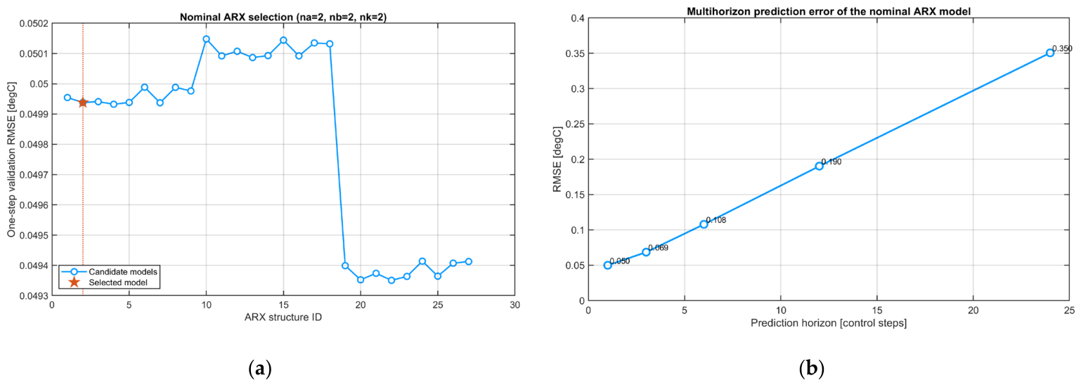
ARX identification was restricted to the approach and holding region. Among 27 candidate structures with $n_a,n_b\in \{2,3,4\}$ and $n_k\in \{1,2,3\}$, the selected model had $n_a=2$, $n_b=2$, and $n_k=2$. It retained discrete-time stability, a positive static gain of 0.0813, and a one-step validation RMSE of 0.0499 °C. The RMSE increased to 0.350 °C at 24 steps, corresponding to 120 s, and to 1.413 °C in free simulation, indicating progressive error accumulation outside measurement-corrected short-horizon prediction. The nominal ARX model was therefore suitable for local receding-horizon control but not for extrapolation across the complete batch cycle or untested operating modes.

Table 6 and Figure 2 provide partial operational support for H1: the hybrid framework combined physical interpretation and plausibility bounds with a stable, parsimonious, and locally predictive ARX model. However, it was not evaluated as a complete model of every batch mode or against all possible modeling alternatives; its validity remains restricted to the experimentally represented region.

4.3. Within-Domain Model-Mismatch Assessment

To examine whether nominal-model performance was concentrated in a narrow batch condition, the independent validation records were stratified according to batch mass and initial temperature. Batch mass was classified as lower, nominal, or higher relative to the campaign distribution, using predefined limits established before calculating the prediction indicators. Initial temperature was similarly divided into lower and higher thermal-load conditions. The nominal ARX coefficients were not re-estimated within these strata.

Table 7. Within-domain prediction robustness of the nominal ARX model.

Operating Stratum	n Batches	Observed Range	1-Step RMSE (°C)	24-Step RMSE (°C)	Free-Simulation RMSE (°C)	Stable Prediction	Interpretation
Lower batch mass	$10$	$242.57-257.27 \mathrm{k}\mathrm{g}$	$0.048$	$0.559$	$1.839$	Yes (positive gain)	Comparable local accuracy; the lowest free-simulation error among the mass strata.
Nominal batch mass	$10$	$257.32-257.60 \mathrm{k}\mathrm{g}$	$0.051$	$0.557$	$1.855$	Yes (positive gain)	Comparable local accuracy; performance was not concentrated in the central mass range.
Higher batch mass	$10$	$257.61-270.42 \mathrm{k}\mathrm{g}$	$0.051$	$0.562$	$1.848$	Yes (positive gain)	Comparable local accuracy; only a negligible increase in the 24-step error was observed.
Lower initial temperature	$15$	$17.53-20.82 °\mathrm{C}$	$0.049$	$0.540$	$1.809$	Yes (positive gain)	Best multi-step and free-simulation accuracy among the initial-temperature strata.
Higher initial temperature	$15$	$20.95-24.46 °\mathrm{C}$	$0.051$	$0.578$	$1.885$	Yes (positive gain)	Slightly higher multi-step errors, without instability or loss of the positive gain sign.

Note: The same fixed nominal ARX model was evaluated in all strata. The strata represent only the variability observed in the experimental campaign and should not be interpreted as validation of the complete equipment operating range.

reports 1-step RMSE, 24-step RMSE, free-simulation RMSE, and the sign and stability of the nominal model across the observed operating strata. This analysis evaluates whether the fixed predictor retained acceptable local performance under the batch-to-batch variability represented in the campaign. It does not extend the empirical validity of the model beyond the observed mass, temperature, agitation, product, or recipe ranges.

4.4. Robustness Assessment Under Parameter Uncertainty and External Disturbances

The offline stress test evaluated whether C3 remained operationally adequate under model–plant mismatch. Unlike the within-domain assessment in Section 4.3, which used variability observed in experimental batches, this analysis introduced parameter uncertainty, measurement uncertainty, effective-delay variation, actuator-gain variability, and temporally correlated residual disturbances. Because C3 is a nominal constrained MPC, the assessment was interpreted as an empirical stress test rather than as proof of robust stability or guaranteed constraint satisfaction.

A total of 400 closed-loop Monte Carlo realizations were generated using MATLAB’s Mersenne Twister pseudorandom-number generator and a fixed base seed of 20260619. The realizations were equally divided into four groups of 100 runs: nominal reference, parameter uncertainty only, external disturbances only, and combined parameter uncertainty and external disturbances. The uncertainty sources and bounds are reported in Table A2.

In every realization, C3 retained the same nominal ARX model, prediction and control horizons, objective-function weights, scaling, actuator and output constraints, solver configuration, and 5 s control period used in the experimental comparison. No online re-identification, retuning, or adaptation was permitted; uncertainty and disturbances were applied only to the simulated plant. The test therefore evaluated tolerance to model–plant mismatch rather than controller reconfiguration.

Table 8. Closed-loop robustness of the nominal constrained MPC under parameter uncertainty and external disturbances.

Scenario Group	Realizations	Feasible QP (%)	Holding Achieved (%)	Maximum Temperature Violation (°C)	RMSE (°C)	Specific Energy Consumption (kWh/kg)	Saturation (%)	Fallback Activations
Nominal model	100	100.0	100.0	0.000	1.451	0.08956	0.00	0
Parameter uncertainty only	100	100.0	100.0	2.552	1.650	0.09592	0.00	0
External disturbances only	100	100.0	100.0	0.038	1.454	0.08943	0.00	0
Combined uncertainty	100	100.0	100.0	1.823	1.615	0.09407	0.00	0
Worst observed metric values	—	—	100.0	2.552	3.678	0.07698	0.00	0

Note: The controller used the fixed nominal ARX model in all realizations. Parameter variations and disturbances were applied only to the simulated plant. Therefore, the analysis evaluated model–plant mismatch rather than controller retuning. The reported results constitute an empirical stress test within the data-derived uncertainty region and not a formal robust-MPC guarantee.

summarizes the resulting closed-loop feasibility, holding-condition attainment, temperature-constraint violation, tracking performance, specific energy consumption, actuator saturation, and fallback behavior for each scenario group.

Across all realizations, the optimization remained feasible at 100.0% of the control instants, and the valid holding condition was achieved in 100.0% of the realizations. Under parameter uncertainty alone, mean RMSE increased from 1.451 °C in the nominal condition to 1.650 °C, while specific energy consumption increased from 0.08956 to 0.09592 kWh/kg. External disturbances produced a mean RMSE of 1.454 °C, indicating only a minor deterioration relative to the nominal reference. The combined uncertainty-and-disturbance scenarios produced a mean RMSE of 1.615 °C and a maximum temperature violation of 1.823 °C. Nevertheless, all simulated trajectories remained bounded, and fallback activation occurred in 0 of the 400 realizations.

The observed changes were physically consistent with variations in effective batch thermal capacity, effective delay, and actuator gain, although the available results do not provide a source-by-source sensitivity ranking. Variations in effective batch thermal capacity primarily altered the heating rate and dominant time constant, whereas effective-delay variation affected the timing of anticipatory power reduction near the holding region. Actuator-gain variability changed the thermal power delivered relative to the MPC command. Correlated residual disturbances produced only small mean changes in tracking, as indicated by the increase in RMSE from 1.451 to 1.454 °C and a maximum temperature violation of 0.038 °C, without a meaningful increase in specific energy consumption. These effects were reflected mainly in RMSE, maximum temperature violation, and specific energy consumption.

Across the complete stress test, the largest observed RMSE was 3.678 °C, whereas the largest observed temperature violation was 2.552 °C. Despite these extrema, C3 maintained optimizer feasibility and bounded trajectories, achieved the valid holding condition, avoided actuator saturation, and did not activate the fallback controller. Because the available summary does not establish that the largest RMSE and largest temperature violation occurred in the same realization, they are interpreted as the worst observed metric values rather than as the results of a uniquely identified worst-case trajectory. These extrema define the practical boundary of the evaluated uncertainty region and indicate that constraint tightening or an explicitly robust MPC formulation would be required before extending operation beyond it.

Overall, C3 tolerated the parameter and disturbance variability represented by the data-derived uncertainty set without loss of optimizer feasibility, trajectory divergence, or failure to attain the valid holding condition. However, these results do not establish robust stability or worst-case constraint satisfaction outside that set. The evidence is therefore restricted to near-nominal fill conditions, the installed sensing and actuation chain, and the 65 °C/30 min milk recipe. Other fill levels, formulations, thermal recipes, severe faults, or substantially different heat-transfer conditions require additional experimental validation or an MPC formulation with explicit uncertainty propagation and constraint tightening.

4.5. Adaptive Observer C1

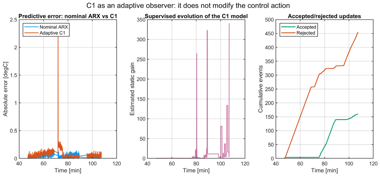
C1 operated as a parallel ARX–RLS observer without modifying the applied power or control law. Its purpose was to separate online parameter estimation from controller-induced performance changes and to screen candidate models before their possible authorization for use by C2 or C4.

A candidate update was accepted only when it satisfied the complete diagnostic framework defined in Table 4, including data eligibility, excitation, numerical conditioning, dynamic stability, physical gain, parameter continuity, spatial consistency, actuator condition, and energy consistency. If any criterion failed, the candidate was rejected, and the previously validated parameter vector was retained. Accordingly, the number of accepted updates indicates numerical and physical admissibility but does not demonstrate predictive or closed-loop superiority over the nominal ARX model.

As shown in

Table 9. Summary of the C1 observer executed without modifying the control action.

Base	n	Nominal ARX RMSE	C1 RMSE	Accepted Updates	Rejected Updates	Acceptance Rate (%)	Dominant Rejection Cause	Stable Final Models (%)
C0	13	0.0579	0.0920	174.5	411.1	29.8	Persistent actuator saturation	100
C2	8	0.0554	0.0820	182.4	433.0	29.6	Persistent actuator saturation	100
C3	13	0.0382	0.0405	271.0	130.2	67.5	Physical-gain criterion	100
C4	8	0.0361	0.0418	218.1	182.4	54.5	Physical-gain criterion	100

Note: Accepted and rejected updates are reported as mean events per batch. Rejection causes were assigned hierarchically according to the first failed diagnostic gate. Stability refers only to the final accepted models and does not imply improved predictive accuracy.

, all final accepted models remained stable under every control base. However, C1 did not reduce predictive RMSE relative to the nominal ARX model in any case. Under C0, RMSE increased from 0.0579 to 0.0920 °C, whereas under C2 it increased from 0.0554 to 0.0820 °C. The differences were smaller under the predictive controllers: RMSE increased from 0.0382 to 0.0405 °C under C3 and from 0.0361 to 0.0418 °C under C4. These results indicate that the fixed nominal ARX model was already informative within the evaluated operating domain and that recursive updating introduced no systematic predictive benefit.

C0- and C2-based operation produced lower acceptance rates and more rejected updates than C3- and C4-based operation. Under C0 and C2, persistent actuator saturation was the dominant first failed diagnostic gate, whereas under C3 and C4 the physical-gain criterion was the dominant rejection cause. This distinction suggests that the admissibility of recursive updates depended not only on the estimator but also on the closed-loop operating conditions generated by the underlying controller.

Figure 3 compares the nominal and adaptive prediction errors, the supervised evolution of the estimated static gain, and the cumulative accepted and rejected update events. Although all final accepted models satisfied the prescribed stability requirements, the C1 RMSE remained above the corresponding nominal-model RMSE for every control base. C1 therefore supported the supervisory component of H3 by demonstrating stable, traceable, and selective update screening, but it did not support the proposition that online adaptation necessarily improves prediction under the limited drift represented in the campaign. The findings confirm that model admissibility is a necessary safety condition but not evidence of predictive or closed-loop benefit.

4.6. Temporal Comparison Between C0 and C3

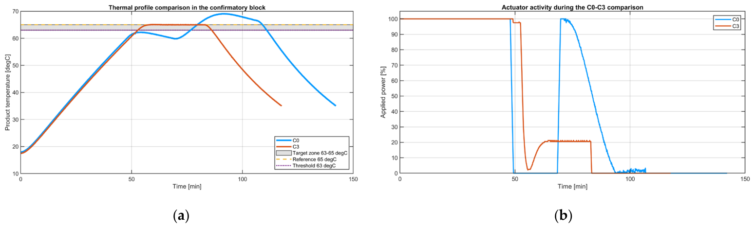
Figure 4 presents a representative block from the confirmatory comparison. C0 reached the holding region with greater overshoot and a more prolonged subsequent thermal excursion. In contrast, C3 reduced power before reaching the setpoint and maintained the product temperature within a narrower band during the holding stage. This visual difference is consistent with the purpose of MPC: to use the fixed nominal ARX model to anticipate the effect of heating power, respect constraints, and avoid delayed corrective actions.

The actuator signal complements the thermal interpretation. C0 maintained high saturation during an important fraction of the batch and then required an abrupt corrective action. C3 applied a progressive power reduction, sustained low levels during holding, and avoided persistent saturation. The improvement did not arise from re-identifying the model during the comparison; the model used by C3 was the previously selected nominal ARX model with fixed parameters. Therefore, the representative block confirms the methodological separation among identification, tuning, and comparison.

4.7. Overall Performance Indicators

Table 10. Mean performance indicators by strategy in batches not used for identification.

Control	n	RMSE (°C)	IAE (°C s)	${\mathit{E}}_{\mathit{s}}$ (kWh/kg)	$\mathit{T}{\mathit{V}}_{\mathit{u}}$	Overshoot (°C)	Sat. (%)	${\mathit{t}}_{\mathit{M}\mathit{P}\mathit{C}}$ (ms)
C0	13	3.207	8886	0.0926	3.926	3.691	45.51	-
C2	8	3.182	9246	0.0938	4.189	3.692	42.61	-
C3	13	1.235	1025	0.0834	1.345	0.098	0.00	6.40
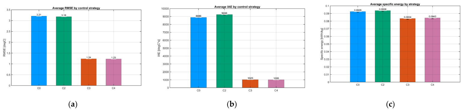
C4	8	1.227	1005	0.0843	1.542	0.111	0.00	6.45

summarizes the mean performance indicators for batches not used for identification. These values are descriptive; confirmatory interpretation is reserved for paired block differences. C0 registered a mean RMSE of 3.207 °C, IAE of 8886 °C s, specific energy consumption of 0.0926 kWh/kg, and saturation of 45.51%. C3 reduced these values to 1.235 °C, 1025 °C s, 0.0834 kWh/kg, and 0% saturation. The simultaneous reduction in tracking error, overshoot, specific energy consumption, and saturation constitutes the clearest descriptive evidence in favor of C3.

C2 showed a slight RMSE reduction relative to C0, but it did not sustain an overall improvement. Its IAE, specific energy consumption, and $T{V}_u$ were higher than those of C0, suggesting that supervised PI self-tuning did not transform the process response robustly enough under slow drift. C4 showed the lowest descriptive RMSE, 1.227 °C, and the lowest descriptive IAE, 1005 °C s; however, its specific energy consumption and $T{V}_u$ were higher than those of C3, as shown in Table 10 and Figure 5. This difference is important for H5: the adaptive extension may marginally improve tracking, but it introduces additional actuator activity and should not be presented as conclusively superior.

4.8. Paired Confirmatory Comparison C3-C0

The confirmatory analysis used five matched blocks, each contributing one batch-level observation for C3 and one for C0. Thus, inference was based on five paired differences rather than on the temporal samples recorded during controller execution.

Table 11. Paired statistical analysis of the confirmatory C3–C0 comparison.

Indicator	C3, Mean ± SD	C0, Mean ± SD	Δ (C3–C0), Mean ± SD	Relative Change vs. C0 (%)	95% CI for Δ	Hedges-Corrected Paired Effect Size	Holm-Adjusted p-Value	Blocks Favoring C3
RMSE (°C)	1.235 ± 0.021	3.194 ± 0.029	−1.959 ± 0.012	−61.3	[−1.974, −1.944]	−128.356	1.09 × 10−9	5/5
IAE (°C s)	1029 ± 36	8830 ± 172	−7801 ± 142	−88.3	[−7977, −7625]	−43.915	5.28 × 10−8	5/5
Specific energy consumption (kWh/kg)	0.0857 ± 0.0024	0.0938 ± 0.0042	−0.0081 ± 0.0041	−8.6	[−0.013, −0.003]	−1.560	0.0121	5/5

Note: Values were calculated from five batch-level paired differences. The paired difference was defined as $\Delta =X_{C3}-X_{C0}$; therefore, negative values favor C3 for indicators in which lower values represent better performance. Relative changes were calculated against C0 using unrounded values. The standardized effect size corresponds to the small-sample-corrected paired effect size defined in Section 3.9. The reported p-values were obtained from paired-samples $t$-tests and adjusted across the three indicators using the Holm procedure. IAE was interpreted as complementary to RMSE because both indicators were derived from the same temperature-error trajectory.

reports controller-specific variability, paired differences, relative changes, 95% confidence intervals, small-sample-corrected paired effect sizes, Holm-adjusted $p$-values, and directional consistency across blocks.

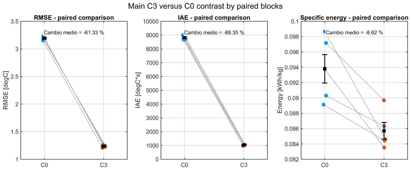
C3 reduced RMSE by 1.959 °C, IAE by 7801 °C s, and specific energy consumption by 0.0081 kWh/kg, corresponding to relative reductions of 61.3%, 88.3%, and 8.6%, respectively. All five paired blocks favored C3 for RMSE and IAE, and all five blocks also favored C3 for specific energy consumption. The energy outcome showed greater relative between-block variability than the tracking indicators. Because RMSE and IAE originated from the same error trajectory, IAE was treated as complementary accumulated-error evidence rather than as an independent confirmation. Overall, the improved temperature regulation was not achieved through greater specific energy use.

Additional engineering indicators are reported in

Table A1. Additional engineering indicators for the paired C3–C0 comparison.

Indicator	C3	C0	Δ (C3–C0)	Reduction Relative to C0 (%)	95% CI for Δ	Interpretation
Actuator total variation, $T{V}_u$	1.398	3.983	−2.585	64.9	[−2.698, −2.472]	Lower actuator activity with C3
Overshoot (°C)	0.111	3.685	−3.573	97.0	[−3.640, −3.506]	Substantial reduction in thermal overshoot
Time outside the admissible band (s)	378	2852	−2474	86.7	[−2513, −2435]	Shorter thermal deviation from the admissible range
Actuator saturation (%)	0.00	44.46	−44.46	100.0	[−47.99, −40.92]	Persistent actuator saturation was eliminated
Thermal overexposure (°C s)	21	4738	−4717	99.6	[−4980, −4454]	Substantial reduction in accumulated exposure above the reference condition

Note: Values correspond to the five paired confirmatory blocks. The paired difference was calculated as $\Delta =X_{C3}-X_{C0}$; therefore, negative values favor C3 for all indicators reported in this table. The percentage reduction was calculated relative to C0 using the unrounded paired estimates. $T{V}_u$ denotes the total variation in the applied control input. Confidence intervals were calculated from the batch-level paired differences rather than from temporally correlated samples.

. Relative to C0, C3 reduced actuator total variation by 64.9%, overshoot by 97.0%, time outside the admissible band by 86.7%, and thermal overexposure by 99.6%, while eliminating persistent actuator saturation. The optimization remained feasible at all evaluated control instants.

Thermal overexposure was not interpreted as microbiological equivalent lethality. The reported values of 4738 °C s for C0 and 21 °C s for C3 represent mean-temperature degree–time exposure above the control reference. Their difference of 4717 °C s indicates substantially lower controller-induced thermal excess, but it cannot be converted uniquely into $F_0$, which depends exponentially on the complete temperature trajectory. Moreover, $F_0$ is referenced to 121.1 °C with $z=10$ °C and is not the appropriate primary microbiological measure for the evaluated 65 °C pasteurization treatment. Target-specific pasteurization values would require validated $D$- and $z$-values and were not used as confirmatory evidence.

Figure 6 shows the paired-block results for RMSE, IAE, and specific energy consumption. The tracking improvement was directionally consistent and was not attributable to a single batch, whereas specific energy consumption exhibited greater dispersion while retaining a mean difference favoring C3. The paired design preserved correspondence between batches operated under matched conditions.

4.9. Secondary and Exploratory Comparisons

C2 and C4 addressed different contrasts and were therefore not combined into a single controller ranking. C2 was compared with C0 as a secondary evaluation of supervised PI retuning, whereas C4 was compared with C3 as an exploratory evaluation of adaptive versus nominal MPC. No paired C2–C3 inference was made.

Table 12. Summary interpretation of secondary and exploratory comparisons.

Contrast	Indicator	Δ	Interpretation
C2–C0	RMSE	−0.039	Support
C2–C0	IAE	442	No support
C2–C0	$E_s$	0.0039	No support
C4–C3	RMSE	−0.0045	Partial support
C4–C3	IAE	−14.9	Partial support
C4–C3	$E_s$	0.0016	No support

summarizes the direction and interpretation of the changes in RMSE, IAE, and specific energy consumption for both contrasts.

Relative to C0, C2 reduced RMSE by 0.0388 °C and saturation by 3.64 percentage points but increased IAE, specific energy consumption, and actuator activity. H3 therefore received partial support: supervised adaptation improved selected tracking and saturation indicators but did not provide an overall performance improvement under drift. The C1 results further showed that online updating requires supervision and rejection of inadmissible parameter estimates.

C4 marginally reduced RMSE and IAE relative to C3 while maintaining feasibility and computation time compatible with the control period. However, it increased specific energy consumption, $T{V}_u$, and thermal overexposure. C4 therefore did not provide a sufficiently balanced advantage to replace C3. Instead, the results support authorizing MPC adaptation only when its predictive or tracking benefit exceeds the associated increases in energy use and actuator activity.

4.10. Hypothesis Synthesis and Validity Domain

Table 13. Hypothesis support within the validated experimental domain.

Hypothesis	Decision	Interpretation
H1	Partial operational support	The ARX model was stable, parsimonious, and characterized by positive gain; the grey-box model provided physical bounds, although energy closure was not exact.
H2	Support	C3 reduced RMSE, IAE, saturation, overshoot, and thermal overexposure relative to C0 without compromising feasibility.
H3	Partial support	C2 reduced RMSE and saturation under drift but increased IAE, energy, and actuator activity; C1 acted as a safe observer, not as a direct improvement.
H4	Partial support	C3 reduced specific energy consumption and thermal overexposure; C2 did not sustain the energy improvement.
H5	Partial exploratory support	C4 slightly reduced RMSE and IAE relative to C3 and maintained computation time, but increased energy use and $T{V}_u$.

synthesizes the hypothesis decisions within the experimentally represented domain. H1 received partial operational support because the hybrid framework combined physical plausibility with a stable, parsimonious, positive-gain ARX predictor, although energy closure was incomplete and alternative model architectures were not exhaustively compared. H2 was supported by the confirmatory C3–C0 results. H3–H5 received partial support because adaptation improved selected indicators but did not provide a consistently superior tracking–energy–actuator trade-off.

Overall, C3 was the preferred nominal predictive strategy for the evaluated pasteurizer, whereas C2 and C4 remained conditional supervised extensions rather than automatic replacements. These conclusions are limited to batches near the nominal fill condition, the installed sensing and actuation architecture, and the 65 °C/30 min milk recipe. Transfer to routine industrial operation requires further validation across broader operating conditions, including sensor and power-system behavior and direct product-quality and microbiological measurements. The operational holding criterion should not be interpreted as microbiological validation or sanitary certification.

5. Discussion

The findings support a process-specific identification–control workflow for a closed, stirred, energy-accumulating pasteurizer. The batch–jacket grey-box model and local ARX predictor played complementary roles, while the nominal constrained MPC–ARX improved tracking, energy use, actuator behavior, and thermal exposure relative to the fixed-parameter PI benchmark. These conclusions apply only to the experimentally represented domain and do not imply universal controller superiority, microbiological validation, or sanitary certification [37,38].

5.1. Interpretation of the Hybrid Grey-Box–ARX Framework

The batch–jacket grey-box model served as a physical and energy-plausibility layer rather than as a high-fidelity simulator. Its estimated thermal capacities and conductance provided interpretable initialization and validation bounds, whereas the relative energy-closure error of 0.234 ± 0.032 reflected unresolved heat losses, metallic thermal storage, power uncertainty, and simplified jacket dynamics. This use is consistent with hybrid approaches that preserve physical structure while estimating plant-specific thermal behavior from data [8,10,14].

The selected ARX model ($n_a=2$, $n_b=2$, and $n_k=2$) was stable, parsimonious, and characterized by positive static gain. Its validation RMSE increased from 0.0499 °C at one step to 0.350 °C at 120 s and 1.413 °C in free simulation. Thus, it was adequate for measurement-corrected receding-horizon prediction in the approach and holding region, but not for the complete batch cycle, rapid heating, cooling, or untested operating modes [30,32,33]. The hybrid framework therefore combined physical interpretability with local predictive capacity without claiming that either model reproduced all plant dynamics.

5.2. Control Performance, Literature Positioning, and Benchmark Scope

In the five paired blocks, C3 reduced RMSE by 1.959 °C, IAE by 7801 °C s, specific energy consumption by 0.0081 kWh/kg, and actuator saturation by 44.46 percentage points relative to C0. Overshoot, time outside the admissible band, actuator activity, and thermal overexposure were also reduced. Because tracking improved while energy use and actuator effort decreased, the benefit was not obtained through more aggressive heating. Rather, the predictor allowed earlier power reduction near the setpoint and limited delayed corrective action in the high-inertia batch.

These findings complement MPC studies in continuous HTST pasteurization, plate-heat-exchanger plants, and simulation-based multivariable milk pasteurization [34,35,36], as well as applications to continuous-flow ohmic heating, extrusion, and drying [3,5,6]. Those systems involve continuous transport, outlet-temperature dynamics, direct heating, or multistate flow behavior. The present contribution is therefore methodological and process-specific: it integrates a batch-specific physical layer, a locally validated ARX predictor, measured active power, three-sensor spatial supervision, explicit adaptive-update gates, and paired batch-level evaluation. It does not propose a new general MPC algorithm.

The C3–C0 comparison was an industrial benchmark rather than a complexity-matched contest. C0 included anti-windup, saturation, input-rate limitation, and bumpless transfer, and both controllers used the same reference, sensors, control period, actuator limits, and paired-block protocol. The results therefore quantify the incremental benefit of prediction and explicit constraint handling over this fixed-parameter PI baseline, but not superiority over gain-scheduled PI, nonlinear PID, robust MPC, or nonlinear MPC.

NMPC could extend the validity domain by representing temperature- and mode-dependent dynamics, but it would require an independently validated nonlinear model, state or disturbance estimation, repeated numerical integration, and nonlinear optimization. It may also be more sensitive to initialization, solver tolerances, model mismatch, and fallback design. By contrast, C3 solved a quadratic program in approximately 6.4 ms within a 5 s control period. A fair future comparison should evaluate PI, gain-scheduled or nonlinear PI, linear MPC, and NMPC under common batches, constraints, objectives, measurements, and fallback rules, while reporting calibration effort, feasibility, computation time, and mismatch sensitivity.

5.3. Interpretation and Limits of Supervised Adaptation

The adaptive strategies addressed different contrasts: C2 was evaluated against C0, whereas C4 was evaluated against C3. Neither provided a sufficiently balanced improvement to replace nominal MPC. C1 further showed that all final accepted models remained stable, although adaptive prediction RMSE exceeded that of the nominal ARX model for every control base. Model admissibility and performance benefit were therefore distinct outcomes.

Several mechanisms explain this result. First, the nominal model already had low local prediction error and the campaign represented limited drift, so any reduction in bias may have been smaller than the additional variance introduced by RLS. Second, closed-loop regulation, actuator constraints, and operation near the holding setpoint reduced persistent excitation and increased regressor correlation. Third, RLS minimized one-step error, whereas controller performance depended on multihorizon prediction, batch-level tracking, energy use, actuator activity, and thermal overexposure. Sensor noise, spatial variation, correlated residuals, and unmodeled jacket dynamics could therefore appear as parameter drift [44].

These mechanisms affected C2 and C4 differently. In C2, changes in estimated gain or dynamics altered PI tuning, producing a slight RMSE and saturation improvement but higher IAE, energy use, and actuator activity. In C4, parameter updates changed the prediction matrices and power sequence; RMSE and IAE improved marginally, but specific energy consumption, actuator variation, and thermal overexposure increased. Thus, adaptation was not uniformly detrimental, but its tracking benefit did not compensate for the wider operational trade-offs [32,33,45].

The supervisory gate rejected invalid, insufficiently excited, ill-conditioned, unstable, physically inadmissible, discontinuous, saturated, spatially inconsistent, or energy-inconsistent updates. It was a safety and model-admissibility filter, not a prospective performance selector. Future authorization should therefore add persistent-mismatch detection, a minimum dwell time, recent-window multihorizon validation, and a performance gate based on a tracking–energy–actuator criterion. Until such conditions are demonstrated, C1 should remain an observer and C3 the default controller.

The fixed-dimensional ARX update also cannot separate slow physical drift from nonlinear or temporally correlated residual dynamics. Hierarchical adaptive estimation and congealed neural-network structures offer conceptual alternatives by separating slowly varying uncertainty from nonlinear residual compensation [49,50,51]. However, their direct application would require a new process model, stability and constraint analysis, additional sensing or state estimation, computational verification, and independent experiments; they motivate future development rather than validate the present ARX–RLS implementation.

5.4. Energy Use, Thermal Exposure, and Industrial Relevance

The simultaneous reductions in error, specific energy consumption, saturation, and actuator activity indicate that C3 used thermal energy more selectively. At the mean batch mass of 257.29 kg, the measured reduction of 0.0081 kWh/kg corresponds to approximately 2.08 kWh per batch. Lower total variation and elimination of persistent saturation may also reduce unnecessary switching and improve power-use traceability.

Thermal overexposure and microbial lethality must nevertheless remain distinct. The former is a linear degree–time measure above the controller reference, whereas equivalent lethality weights the complete temperature trajectory exponentially using a target-specific reference temperature and $z$-value. Consequently, the 99.6% reduction in thermal overexposure cannot be converted through a universal factor into an equivalent reduction in lethality or microbial log reduction. The reported indicator was also based on mean product temperature, while conservative lethality assessment requires a validated cold-point trajectory.

Likewise, $F_0$ is referenced to 121.1 °C with $z=10$ °C and is principally a sterilization metric, not the appropriate primary microbiological criterion for the evaluated 65 °C milk treatment. A target-specific pasteurization value requires validated $D$- and $z$-values, an appropriate reference temperature, and cold-point verification. The observed reduction should therefore be interpreted as lower controller-induced thermal excess, with possible energy and quality implications, not as evidence of microbial safety or sanitary certification [2,37].

Using the illustrative Quito energy-charge range, the measured reduction represents approximately USD 0.13–0.27 per batch and USD 131–274 over 1000 equivalent batches; the corresponding avoided emissions are approximately 0.70 kg CO₂-eq per batch and 0.70 t CO₂-eq over 1000 batches [52,53]. These are order-of-magnitude scenarios, not validated scale-up or life-cycle results. Actual benefits depend on tariff and demand charges, production frequency, geometry, heating efficiency, utility integration, capital and maintenance requirements, and preservation of the specific reduction at larger scale.

5.5. Robustness, Transferability, and Validity Limits

Within the observed batch-mass and initial-temperature strata, the fixed nominal predictor retained stable, positive-gain behavior and comparable 1-step and 24-step accuracy without re-estimation. Errors increased in free simulation, confirming that mismatch accumulated without measurement correction. The offline stress test extended this assessment by applying data-derived parameter, actuator-gain, delay, measurement, and correlated-residual uncertainty only to the simulated plant while retaining the C3 model and tuning.

Across 400 realizations, optimization remained feasible at all control instants, holding was achieved in all realizations, trajectories remained bounded, and neither saturation nor fallback activation occurred. Mean RMSE increased from 1.451 °C nominally to 1.650 °C under parameter uncertainty and 1.615 °C under combined uncertainty and disturbances; external disturbances alone produced only a small change to 1.454 °C. Parameter uncertainty therefore had the larger aggregate effect, although the design did not support ranking individual uncertainty sources. Receding-horizon feedback and input constraints plausibly limited error accumulation but could not compensate indefinitely for large gain or delay errors, severe disturbances, or operation outside the locally identified region.

C3 remains a nominal MPC: it does not use invariant tubes, min–max optimization, chance constraints, or formal uncertainty propagation. The findings demonstrate empirical tolerance within the observed and data-derived uncertainty region, not robust stability or guaranteed worst-case constraint satisfaction. Explicit guarantees would require, for example, constraint tightening, disturbance-state augmentation, gain-scheduled predictors, or tube-based, min–max, or stochastic MPC.

Transferability applies to the workflow rather than to the identified parameters. For a similar closed, stirred, indirectly heated jacketed vessel, the conservation structure may be retained, but thermal capacities, conductance, heat losses, actuator mapping, delay, sensor dynamics, ARX coefficients, constraints, and tuning must be recalibrated and independently validated. Capacity changes require reparameterization rather than proportional scaling because thermal mass, heat-transfer area, surface-to-volume ratio, circulation, and actuator effectiveness do not scale uniformly. Direct-steam, spray, immersion, rotating, pressurized, or continuous systems require partial or complete reconstruction of the physical and predictive models.

Table A4. Transferability and engineering calibration requirements for different target systems.

Transfer Case	Grey-Box Equations	Parameters	ARX Model	MPC Tuning and Constraints	Relative Engineering Effort
Same pasteurizer, similar recipe and fill	Retained	Verification or limited recalibration	Validate or locally update	Verify	Low to moderate
Same pasteurizer, different recipe or fill	Retained, with property-dependent terms reviewed	Recalibrate	Re-identify	Retune and validate	Moderate
Geometrically similar jacketed vessel with different capacity	Retained in structure	Full reparameterization	Re-identify	Retune and validate	Moderate to high
Different indirectly heated batch vessel	Modify according to jacket and service configuration	Full estimation	Re-identify	Redesign constraints and tuning	High
Direct-steam, spray, immersion, rotating, or pressurized retort	Partial or complete reconstruction	New parameter set	New local predictor	New controller validation	High
Continuous pasteurization system	Complete reconstruction	New flow and transport parameters	New dynamic model	New controller architecture	Very high

Note: Relative effort refers to modeling, instrumentation, experimental commissioning, controller calibration, and validation requirements. It does not represent a monetary estimate.

summarizes the relative engineering effort; monetary costs and person-hours were not measured.

The principal validity limitation is that batches were concentrated near nominal fill and all confirmatory comparisons used milk with the 65 °C/30 min recipe. The study did not cover the complete 150–250 L range, other recipes or formulations, severe faults, or substantially altered heat transfer, and the local predictor should not be extrapolated to rapid heating, cooling, or transitions. Statistical generalization is also restricted by five paired confirmatory blocks, although treating the batch as the experimental unit avoided temporal pseudoreplication. Finally, the benchmark was not complexity matched, and no direct microbiological, sensory, physicochemical, or nutritional validation was performed. These restrictions delimit, but do not invalidate, the within-domain comparison.

5.6. Practical Implications and Future Work

Implementation should follow a staged sequence: verify instrumentation, active power, synchronization, agitation, and spatial uniformity; calibrate the batch–jacket grey-box model as a plausibility layer; identify and independently validate the local ARX predictor under safe excitation; and evaluate controllers under common references, constraints, sampling, sensors, and exclusion rules. Within the validated domain, C3 should remain the primary predictive strategy, with C1 operating as an observation layer before any adaptive controller is authorized.

Future blocked campaigns should cover predefined fill levels, initial temperatures, product-specific recipes, agitation and heat-transfer degradation, sensor and actuator uncertainty, and longer operation. They should combine model-validation, feasibility, tracking, energy, actuator, spatial-uniformity, microbiological, product-quality, and metrological outcomes. Broader operation could then be assigned to a common model, gain-scheduled local models, supervised re-identification, or an explicitly robust controller.

Further work should also compare linear MPC with gain-scheduled PI and NMPC under common experimental conditions and conduct plant-specific techno-economic and environmental assessment. A longer-term extension is a hierarchical robust adaptive architecture combining nominal MPC, supervised estimation of slow physical drift, bounded residual-dynamics compensation, independent safety and performance authorization, and fallback control [49,50]. Such an architecture requires process-specific stability analysis, explicit constraint treatment, computational verification, and experimental validation.

6. Conclusions

This study developed and experimentally evaluated a traceable hybrid grey-box–ARX identification and constrained-control workflow for a 250 L jacketed batch milk pasteurizer. The plant was treated as a closed, stirred, energy-accumulating batch system rather than as a continuous HTST process. This distinction determined the model structure, signal selection, interpretation of thermal holding, and use of the complete batch—not temporally correlated samples—as the experimental and statistical unit.

The batch–jacket grey-box model and local ARX predictor served complementary purposes. The grey-box model provided physical interpretation, energy-consistency bounds, and parameter initialization, whereas the selected $n_a=2$, $n_b=2$, and $n_k=2$ ARX structure supplied a stable, parsimonious, positive-gain predictor for the approach and holding region. Its low one-step error supported receding-horizon control, while the increase in multihorizon and free-simulation errors confirmed that the model should not be extrapolated to the complete batch cycle, rapid transitions, cooling, or untested operating modes.

In five paired confirmatory blocks, C3, the nominal constrained MPC–ARX strategy, improved performance relative to the fixed-parameter PI controller with anti-windup. C3 reduced RMSE by 1.959 °C, IAE by 7801 °C s, and specific energy consumption by 0.0081 kWh/kg. It also reduced overshoot, time outside the admissible band, actuator activity, saturation, and thermal overexposure. Optimization remained feasible at all evaluated experimental control instants, with a mean solution time of approximately 6.4 ms within the 5 s control period. C3 was therefore the preferred predictive strategy within the evaluated domain. This conclusion is restricted to the fixed-parameter PI benchmark used in the paired campaign and does not establish superiority over gain-scheduled PI, nonlinear control, robust MPC, or NMPC.

Supervised adaptation provided diagnostic and exploratory value but did not establish an overall advantage over the nominal model and controller. C1 screened ARX–RLS updates for data eligibility, excitation, conditioning, stability, physical admissibility, parameter continuity, and energy consistency, yet accepted updates did not systematically improve prediction. C2 and C4 produced limited improvements in selected tracking indicators but introduced unfavorable trade-offs in accumulated error, energy use, actuator activity, or thermal overexposure. Adaptation should therefore remain a conditional extension rather than an automatic replacement for C3. Under the limited drift and closed-loop excitation represented in the campaign, the potential reduction in model bias was insufficient to offset estimation variability and the propagation of parameter changes into controller behavior.

The within-domain assessment and data-derived stress test provided additional evidence that C3 tolerated the represented parameter, actuator-gain, delay, measurement, and correlated-disturbance variations while maintaining feasible and bounded closed-loop operation and attaining the valid holding condition. However, C3 remains a nominal MPC; these results demonstrate empirical tolerance to model–plant mismatch within the evaluated uncertainty region, not formal robust stability or guaranteed worst-case constraint satisfaction. Likewise, the reduction in degree–time thermal overexposure indicates lower controller-induced thermal excess but is not equivalent to a reduction in accumulated microbial lethality. Target-specific lethality requires a validated cold-point trajectory and appropriate reference-temperature, $D$-value, and $z$-value information. No microbial log-reduction, $F_0$-based sterilization, product-quality, or sanitary-certification claim is therefore inferred.

The conclusions are limited to the evaluated pasteurizer, batches concentrated near nominal fill, the installed sensing and actuation chain, and the 65 °C/30 min milk recipe. The complete 150–250 L fill range, alternative products and recipes, severe faults, and substantially different heat-transfer conditions were not experimentally validated. Transferability consequently applies to the workflow rather than to direct reuse of plant-specific parameters: similar jacketed vessels require parameter recalibration, ARX re-identification, controller retuning, robustness assessment, and independent closed-loop validation, whereas different heating or transport architectures require partial or complete model reconstruction. Future blocked campaigns should extend validation across predefined fill levels, recipes, disturbances, and longer operating periods; incorporate direct microbiological and product-quality measurements; compare linear MPC with gain-scheduled PI and NMPC under common conditions; and conduct plant-specific techno-economic and environmental assessments. More advanced hierarchical or neural robust adaptive structures should be considered only after process-specific stability, constraint, computational, and experimental validation.