Physical Experiment of Gas–Liquid Two-Phase Flow in Vertical Wellbores and Optimization of Pressure Drop Prediction Models


Abstract
1. Introduction
2. Design and Results of Physical Experiment on Gas–Liquid Two-Phase Flow in Vertical Wellbore
2.1. Experimental Apparatus and Experimental Design
2.2. Experimental Procedure
- (1)
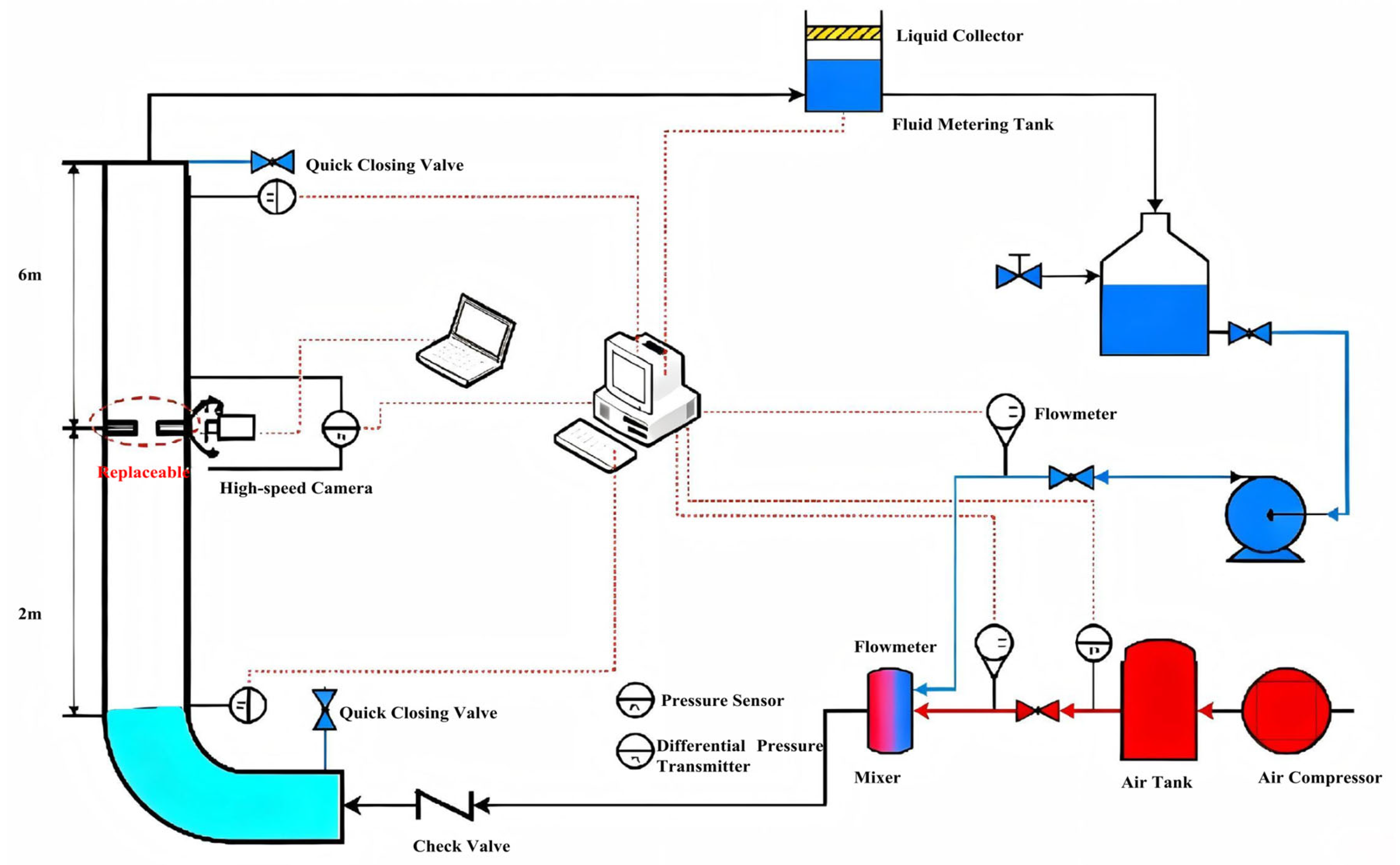
- System startup and gas flow rate regulation: Open the air inlet valve of the storage tank and the air compressor, start the data acquisition system (sampling frequency: 1 Hz), and record the initial environmental parameters. Adjust the pneumatic valve so that the gas flow rate stabilizes within ±2% of the target value. After maintaining stability for 2 min, record the reading of the gas flowmeter.
- (2)
- Liquid flow rate regulation and two-phase mixing: Open the outlet valve of the liquid storage tank, start the liquid flowmeter, and then adjust the liquid branch valve to set the liquid flow rate to the desired values (0.5, 1.0, 1.5 m3/d). After the gas and liquid phases are thoroughly mixed in the mixer and enter the vertical test section, observe the flow state in the section and wait for the flow parameters (pressure, temperature, and flow rate) to stabilize (stability criterion: fluctuations of each parameter within ±1% of the set value over 2 min).
- (3)
- Flow pattern imaging and data acquisition: Once stabilized, activate the high-speed camera to capture gas–liquid flow pattern images through the transparent window of the test section. Annotate the operating condition number, time, pipe diameter, and inclination angle, and preliminarily determine the flow pattern type based on the visual images. Simultaneously, continuously acquire pressure, temperature, differential pressure, and flow rate data for 3 min, and take the arithmetic mean values as the steady-state values for that operating condition.
- (4)
- Liquid holdup measurement (quick-closing valve method): Immediately after completing data acquisition for each steady-state condition, perform liquid holdup measurement. A set of pneumatic quick-closing valves (response time < 0.1 s) is installed upstream and downstream of the test section. While keeping the gas and liquid flow rates unchanged, trigger both quick-closing valves to close simultaneously, trapping the gas–liquid mixture in the test section of known length. Then open the drain valve to discharge the trapped liquid into a measuring cylinder, read the liquid volume, and calculate the average liquid holdup based on the inner diameter and length of the test section. Repeat the measurement three times for each condition and take the average value as the experimental liquid holdup for that flow pattern. After measurement, reopen the quick-closing valves to resume flow, and wait for stabilization before adjusting the flow rates for the next set of conditions.
- (5)
- Repetition of the same condition and traversing multiple conditions: After completing one set of conditions, first adjust the liquid flow rate to the next set value and allow stabilization, then fine-tune the pneumatic valve to calibrate the gas flow rate. Repeat steps (2)–(4) to complete all preset liquid–gas ratio tests under the same pipe diameter and inclination angle. Thereafter, change the pipe diameter (40, 60, or 75 mm) or adjust the inclination angle (0–90°), and repeat the above procedures of gas/liquid regulation, data acquisition, and liquid holdup measurement.
- (6)
- Experiment termination and system cleaning: After all test conditions are completed, close the liquid valve, gas valve, pneumatic valves, and compressor in sequence, and slowly release the storage tank pressure to atmospheric pressure. Turn on dry air purging to remove residual liquid from the test section. Turn off all power supplies, organize the experimental data, and clean the bench.
2.3. Experimental Uncertainty Analysis
2.4. Analysis of Experimental Results
2.4.1. Analysis of Experimental Flow Patterns
2.4.2. Analysis of Liquid Holdup Results
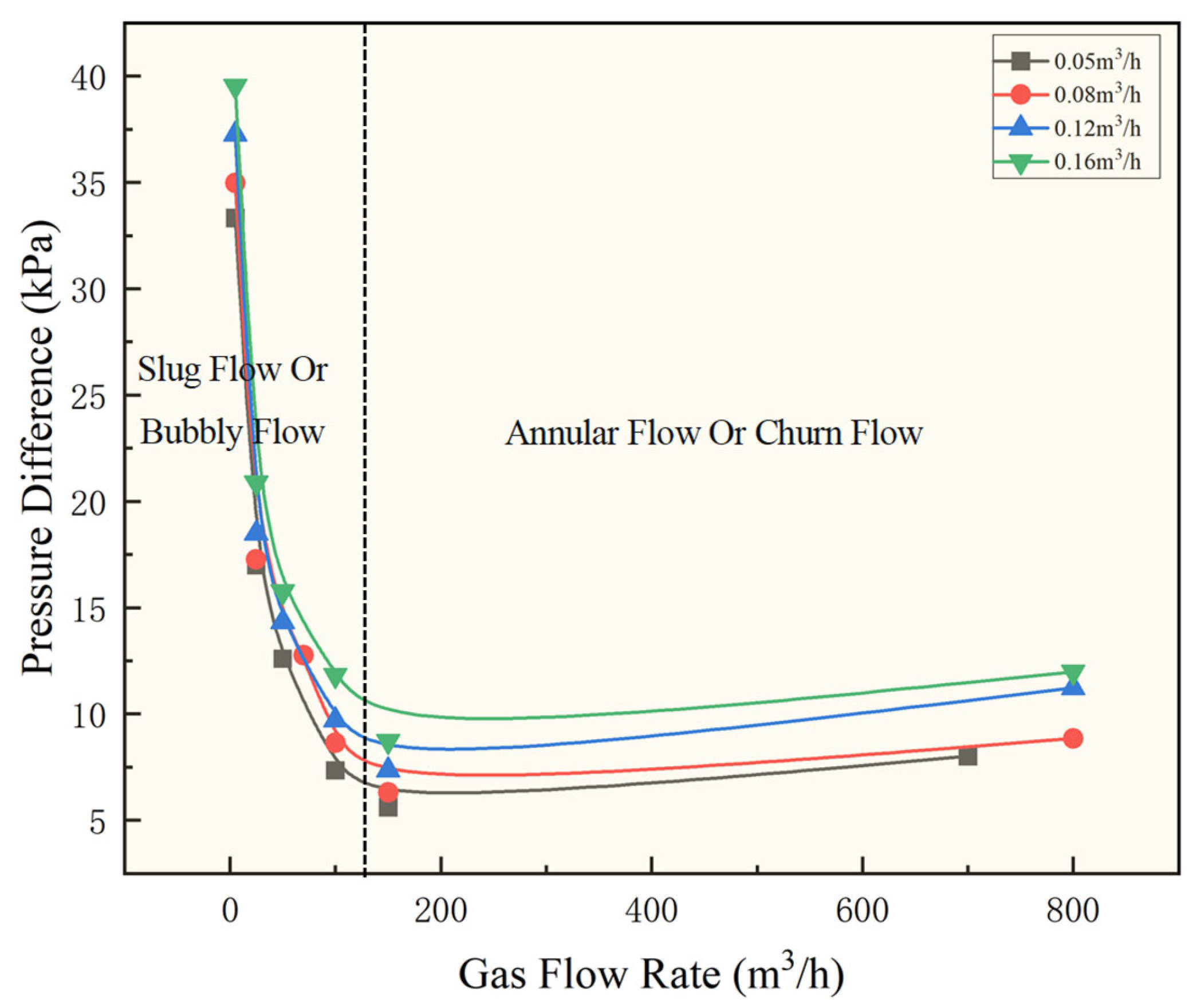
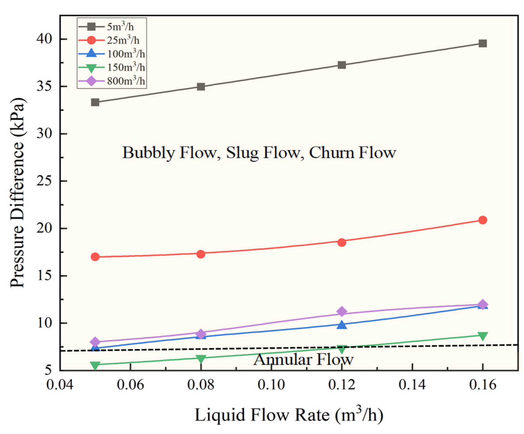
2.4.3. Analysis of Pressure Drop Results
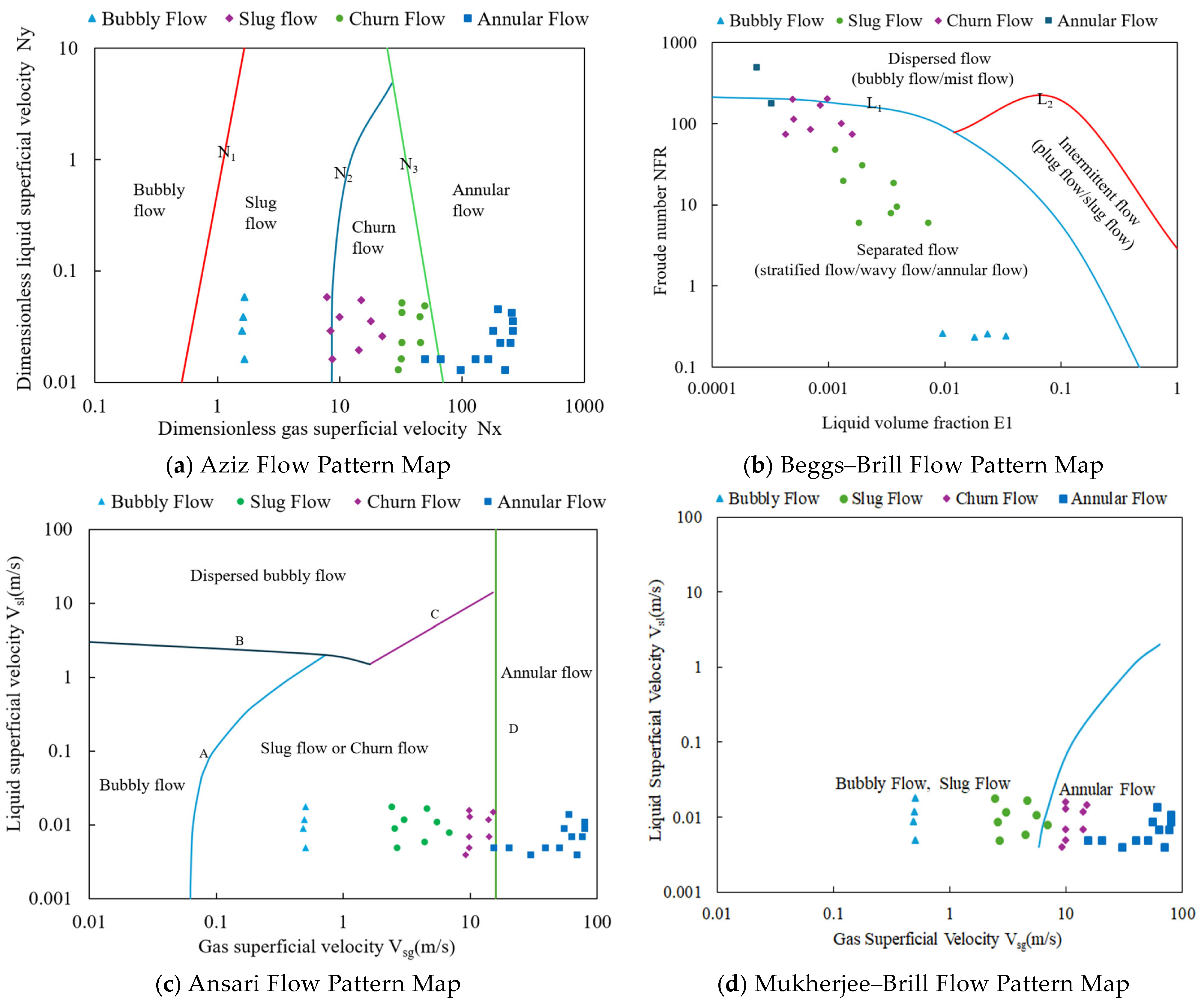
3. Model Selection for Flow Pattern Discrimination of Gas–Liquid Two-Phase Flow in Vertical Wellbores
4. Correction and Optimization of Pressure Drop Prediction Models for Vertical Wellbores
4.1. Calculation Methods of Pressure Drop for Different Flow Patterns
- (1)
- For bubbly flow, Aziz et al. (1972) [6] proposed the pressure drop formula given by Equation (7):
- (2)
- For slug flow, Aziz et al. proposed the pressure drop formula given by Equation (10).
- (3)
- For annular flow, the Duns Ros [27] method should be adopted for calculation according to Region III, as shown in Equation (11).
- (4)
- For churn flow, the pressure gradient must be calculated using a linear weighting of the formulas for slug flow and annular flow simultaneously, as shown in Equation (12).
4.2. Correction of the Pressure Drop Prediction Model for Vertical Wellbores
4.2.1. Principle of Particle Swarm Optimization Algorithm
4.2.2. Model Calibration Using Particle Swarm Optimization
- (1)
- The calculation formula for bubbly flow is shown in Equation (16).
- (2)
- The calculation formula for slug flow is shown in Equation (17).
- (3)
- The calculation formula for churn flow is shown in Equation (18).
- (4)
- The calculation formula for annular flow is shown in Equation (19).
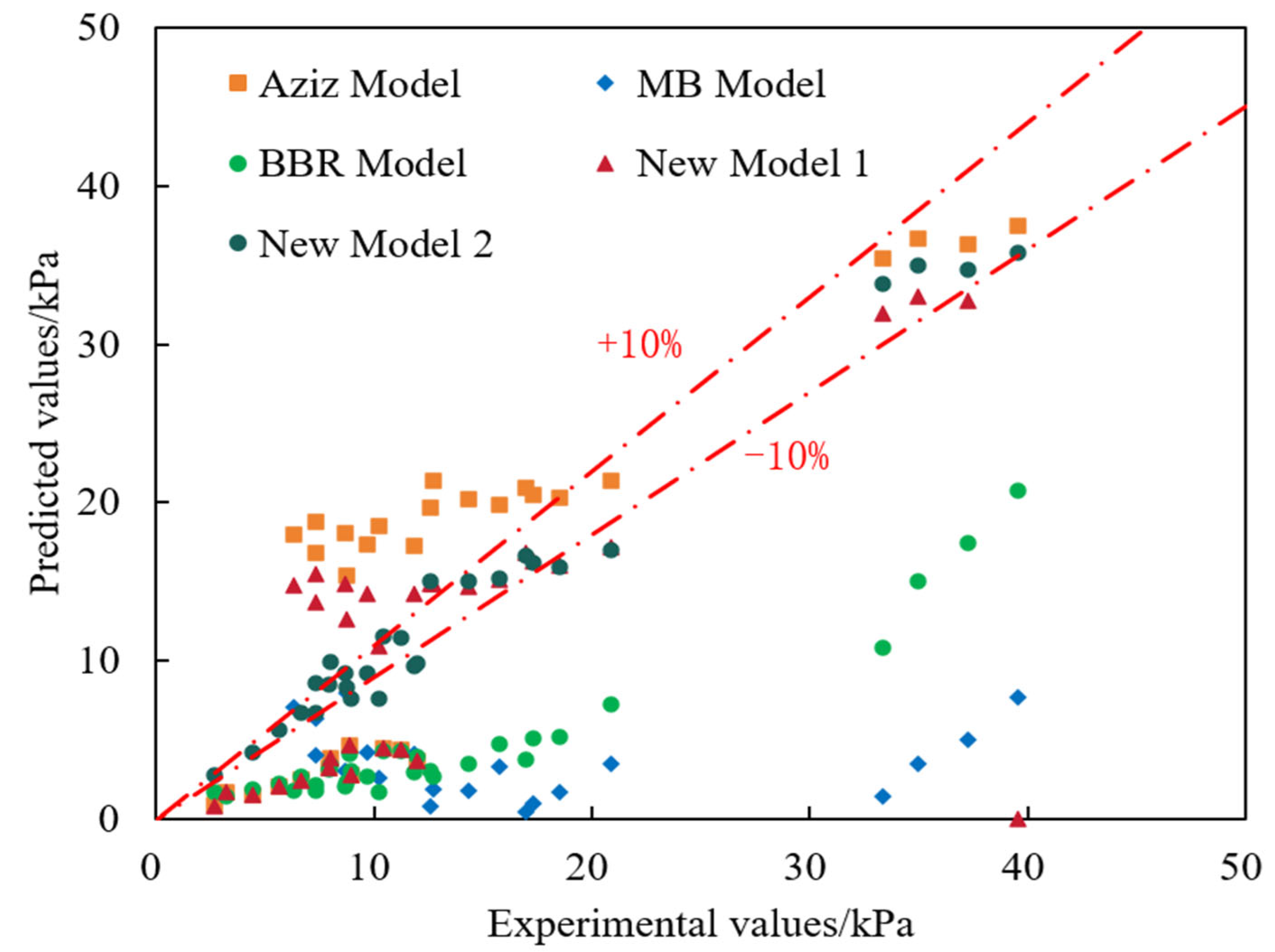
4.3. Evaluation of the Pressure Drop Prediction Model for Vertical Wellbores
4.4. New Model 2 Validation
5. Conclusions
- (1)
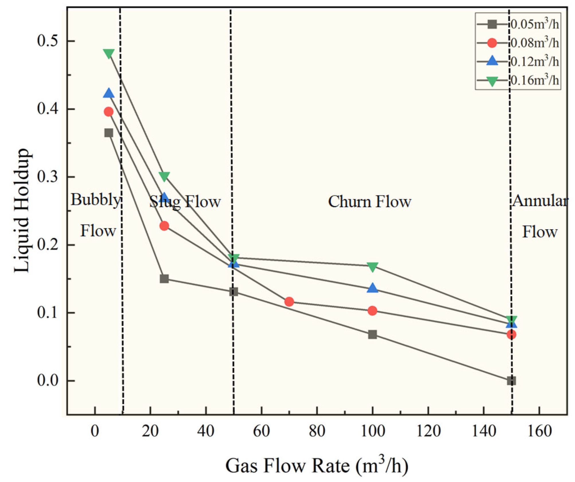
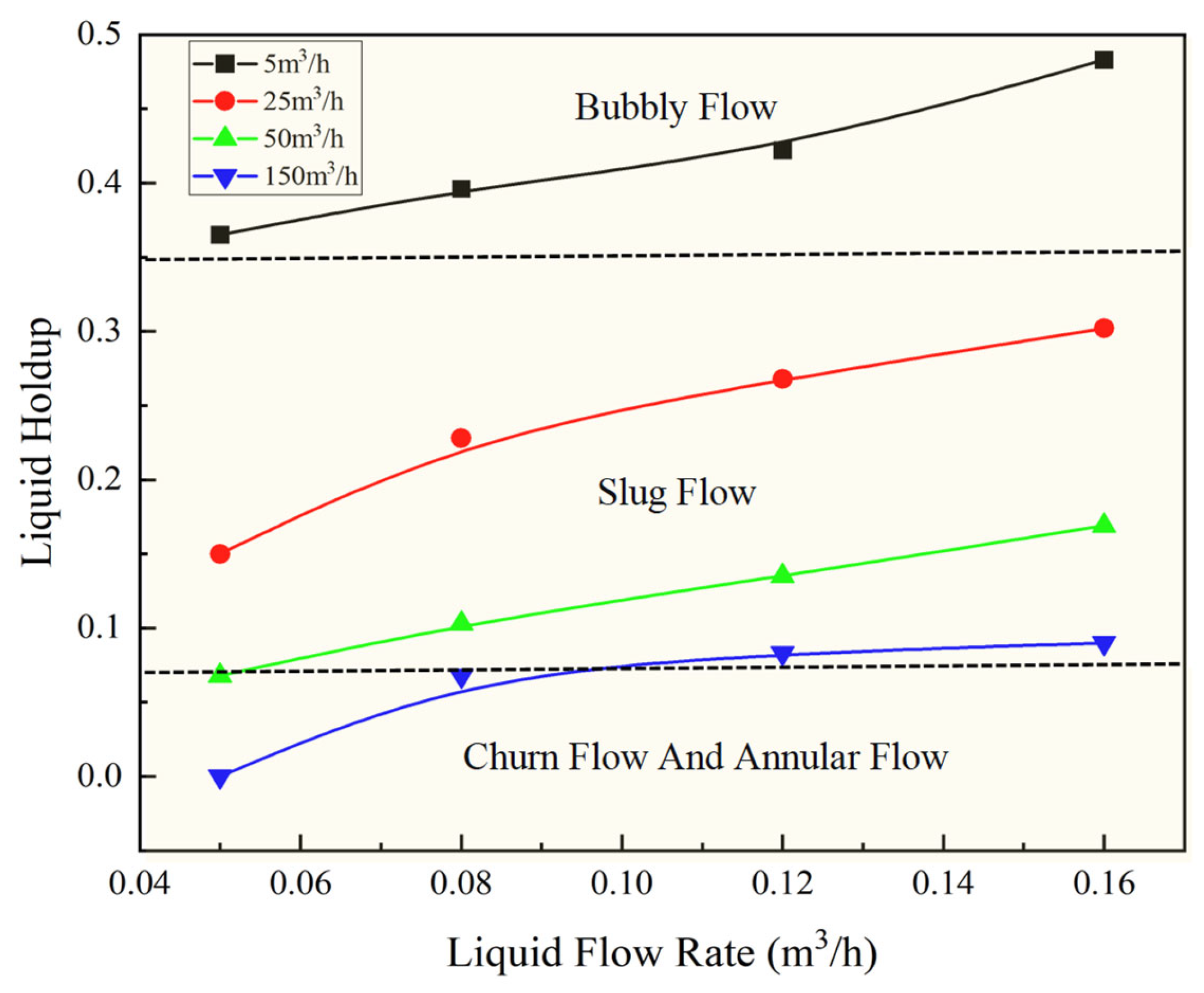
- Through segmented simulation of the gas flow velocity variation from the bottomhole to the wellhead, the four typical flow patterns—bubbly flow, slug flow, churn flow, and annular flow—were clearly observed and recorded on the experimental platform. The transition boundaries among these flow patterns were determined based on daily gas production rate, gas velocity, liquid holdup, and liquid–gas ratio, providing a reliable data foundation for flow pattern identification and model validation.
- (2)
- A comparison of four classical flow pattern identification models—Aziz, Beggs–Brill, Mukherjee–Brill, and Ansari—revealed that the Aziz model provides the most complete coverage of all four flow patterns and exhibits the highest consistency between predicted results and experimental observations. Therefore, it can be recommended as the preferred model for flow pattern identification in vertical wellbores.
- (3)
- To address the substantial pressure drop prediction errors of the original Aziz model, we calibrated the liquid holdup and friction factor using experimental data. Furthermore, the particle swarm optimization (PSO) algorithm was employed for optimal fitting, with the correction coefficients systematically adjusted to minimize the global error. A new pressure drop prediction model (referred to as Model 2) applicable to different flow patterns was thereby established. This model significantly improves the prediction accuracy, achieving an overall MAPE of 11.9% and an RMSE of 1.9 kPa. Model 2 yields an average MAPE of 12.0% on the independent validation dataset, maintaining satisfactory accuracy beyond the parameter calibration set. Compared with the classical Aziz model (MAPE of 50.6%, RMSE of 5.3 kPa) and the manually calibrated Model 1 (MAPE of 18.2%, RMSE of 4.9 kPa), the proposed model demonstrates a considerable improvement in prediction accuracy.
Author Contributions
Funding
Data Availability Statement
Conflicts of Interest
References
- Zhang, L. Application of bottom hole pressure calculation method for gas well with downhole throttling. J. Chengde Pet. Coll. 2022, 24, 34–39. [Google Scholar] [CrossRef]
- Liu, S.; Wang, H.; Luo, Y.; Wang, D.; Hu, Y.; Zhu, Z. A new method for determining the bottom hole pressure of downhole throttled gas wells. J. Xi’an Shiyou Univ. (Nat. Sci. Ed.) 2012, 27, 53–56. [Google Scholar] [CrossRef]
- Wang, H.; Yi, X.; Lu, Y. Status of research on vertical conduit flow of gas-liquid two phases in wellbore. Xinjiang Pet. Geol. 2006, 27, 740–742. [Google Scholar] [CrossRef]
- Liu, X.; Xu, Y.; Peng, H.; Mu, Q.; Cui, K.; Cao, X. Mechanistic modeling of two-phase flow in deviated wells. Oil Drill. Prod. Technol. 2009, 31, 52–57. [Google Scholar] [CrossRef]
- Li, S. Natural Gas Engineering; Petroleum Industry Press: Beijing, China, 2000. [Google Scholar]
- Aziz, K.; Govier, G.W. Pressure drop in wells producing oil and gas. J. Can. Pet. Technol. 1972, 11, 38–48. [Google Scholar] [CrossRef] [Scilit]
- Beggs, D.H.; Brill, J.P. A Study of two-phase flow in Inclined pipes. J. Pet. Technol. 1973, 25, 607–617. [Google Scholar] [CrossRef] [Scilit]
- Mukherjee, J. Pressure drop correlations for inclined two-phase flow. J. Energy Resour. Technol. 1985, 107, 549–554. [Google Scholar] [CrossRef] [Scilit]
- Ansari, A.; Sylvester, N.; Shoham, O. A comprehensive mechanistic model for upward two-phase flow in wellbores. Softw. Pract. Exp. 1994, 9, 143–151. [Google Scholar] [CrossRef]
- Chen, J. Pressure drop calculation for vertical flow of oil, gas, and water mixtures—Flow pattern-based calculation method. Pet. Explor. Dev. 1980, 7, 55–67. Available online: https://xuebao.nepu.edu.cn/info/1147/9643.htm (accessed on 24 June 2026). [CrossRef] [Scilit]
- Gao, S.; Liu, Y.; Zhang, Y.; Lai, X.; Li, S.; Luo, C.; Wang, W. The forecast and analysis of pressure of gas well of western sichuan gas field. J. Chongqing Univ. Sci. Technol. (Nat. Sci. Ed.) 2012, 14, 60–63. [Google Scholar] [CrossRef]
- Liu, T.; Wang, S.; Guo, X.; Pan, G.; Chen, H.; Wu, Z. New calculation method of gas-liquid two phase annular-mist flow pressure drop of wellbores in gas wells. Oil Drill. Prod. Technol. 2017, 39, 328–333. [Google Scholar] [CrossRef]
- Liu, Z.; Liao, R.; Lei, Y.; Wu, Z.; Zhao, Y. Pressure drop model of oil-gas two-phase flow in horizontal pipes with different diameters. Sci. Technol. Eng. 2019, 19, 137–143. [Google Scholar] [CrossRef]
- Liu, Y.; Bai, X.; Cheng, Y.; Wang, X.; Song, H.; Liang, R. Experimental study on pressure drop of gas-liquid two-phase flow in inclined annulus pipe. China Sci. Pap. 2020. [Google Scholar] [CrossRef]
- Cheng, Y.; Wu, H.; Chen, Y.; Liao, R. Experimental study on changing laws of pressure drop of gas liquid two phase flow in horizontal wells. China Energy Environ. Prot. 2019, 41, 68–72+116. [Google Scholar] [CrossRef]
- Wang, G. Study of Gas Wellbore Flow Dynamics in the Ma Xian Area. Master’s Thesis, Yangtze University, Jingzhou, China, 2023. [Google Scholar] [CrossRef]
- Li, L. Prediction of Liquid Holdup and Pressure Drop in Gas-Liquid Two-Phase Flow Based on Neural Network. Master’s Thesis, Yangtze University, Jingzhou, China, 2024. [Google Scholar] [CrossRef]
- Liu, Z.; Qian, X.; He, J.; Liao, R.; Chen, C. Pressure drop prediction model for vertically upward annular flow in annular space of oil tube and casing. Pet. Drill. Tech. 2025, 53, 16–125. [Google Scholar] [CrossRef]
- Lin, J.; Li, H.; Liu, Y.; Xu, S.; Liu, Y.; Cao, Y. Modeling studies on pressure gradient prediction for shale horizontal gas wells. Oil Field Equip. 2025, 54, 6–11. [Google Scholar] [CrossRef]
- Zeng, Q.; Hao, X.; Sui, T.; Xu, L.; Wang, Z.; Gao, W. Predictive method and its application of pressure drop in horizontal wellbore completion string with sliding sleeves. Spec. Oil Gas Reserv. 2024, 31, 159–165. [Google Scholar] [CrossRef]
- Osman, E.S.A. Artificial neural network models for identifying flow patterns and predicting liquid holdup in horizontal multiphase flow. SPE Prod. Facil. 2004, 19, 33–40. [Google Scholar] [CrossRef]
- Kanin, E.A.; Osiptsov, A.A.; Vainshtein, A.L.; Burnaev, E.V. A predictive model for steady-state multiphase pipe flow: Machine learning on lab data. J. Pet. Sci. Eng. 2019, 180, 727–746. [Google Scholar] [CrossRef] [Scilit]
- Ribeiro, J.X.F.; Liao, R.; Aliyu, A.M.; Yeung, H. Prediction of pressure gradient in two and three-phase flows in vertical pipes using an artificial neural network model. Int. J. Eng. Technol. Innov. 2019, 9, 155–170. [Google Scholar] [CrossRef] [Scilit]
- Chaari, M.; Ben Hmida, J.; Seibi, A.C.; Al-Abdeli, Y.M. An integrated genetic algorithm artificial neural network approach for steady-state modeling of two-phase pressure drop in pipes. SPE Prod. Oper. 2020, 35, 628–640. [Google Scholar] [CrossRef] [Scilit]
- Zhou, D.; Liao, R.; Wang, W.; Yang, Z. Optimization of the pressure drop prediction model of wellbore multiphase flow based on simultaneous perturbation stochastic approximation. Int. J. Heat Technol. 2022, 40, 1397–1403. [Google Scholar] [CrossRef] [Scilit]
- Faraji, F.; Santim, C.; Chong, P.L.; Parsi, M.; Kim, S. Two-phase flow pressure drop modelling in horizontal pipes with different diameters. Nucl. Eng. Des. 2022, 395, 111863. [Google Scholar] [CrossRef] [Scilit]
- Duns, H.; Ros, N. Vertical flow of gas and liquid mixtures in wells. In Proceedings of the 6th World Petroleum Congress, Frankfurt am Main, Germany, 19–26 June 1963. [Google Scholar]
- Chen, J. Oil-Gas Two-Phase Pipe Flow; Petroleum Industry Press: Beijing, China, 1989. [Google Scholar]



| Equipment | Measurement Range | Measurement Accuracy/% |
|---|---|---|
| Pressure Sensor | 0–3.5 MPa | ±0.1 |
| Temperature Sensor | 0–90 °C | ±0.5 |
| Liquid Flowmeter | 2–20 m3/h | ±0.3 |
| Gas–liquid Flowmeter | 160–2000 m3/h | ±1 |
| Parameters | Tubing Inner Diameter (mm) | Liquid–Gas Ratio (m3/104 m3) | Liquid Production Rate (m3/d) | Gas Production Rate (104 m3) |
|---|---|---|---|---|
| Average | 62 | 0.77 | 0.39 | 0.6 |
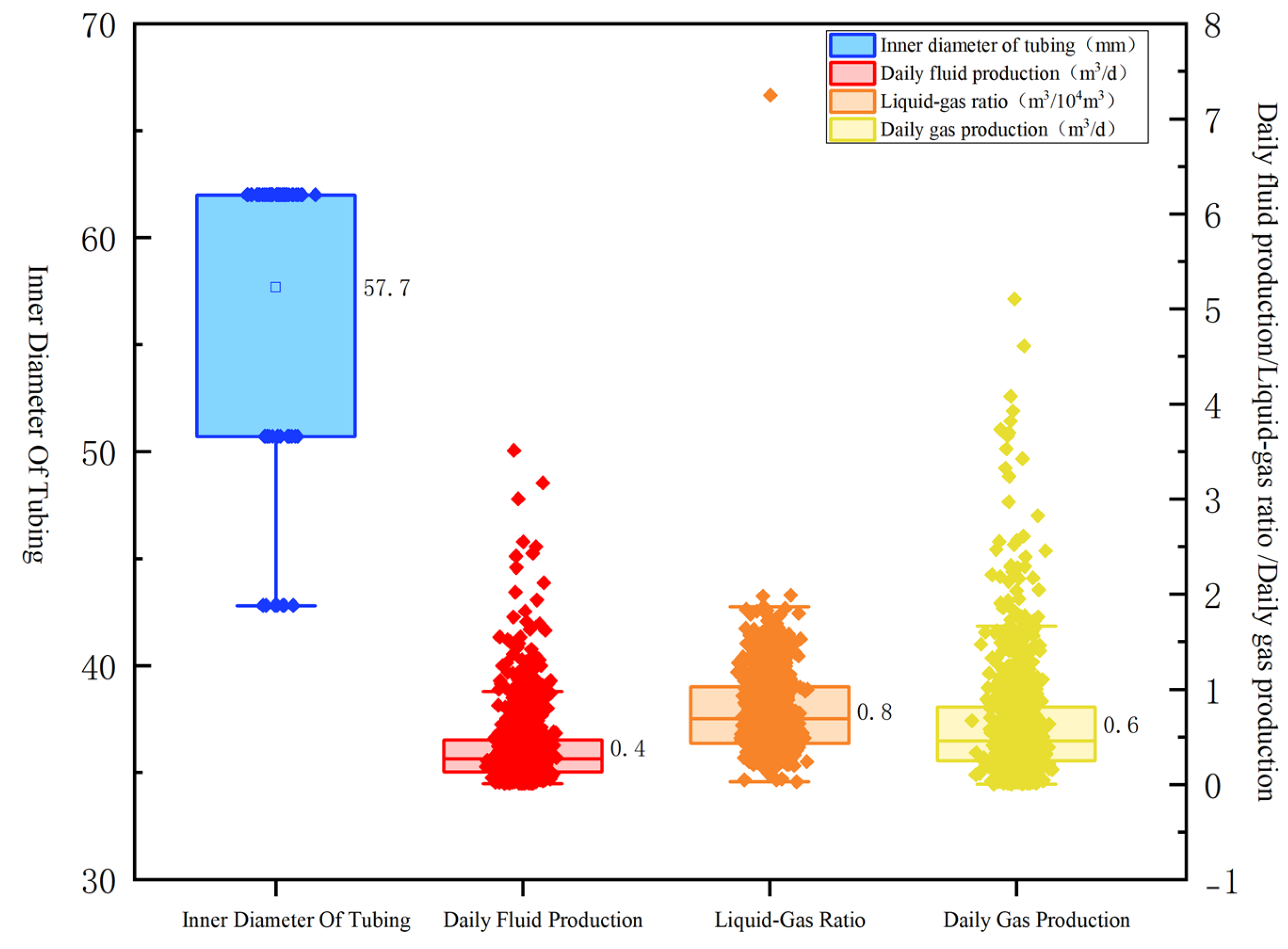
| Experimental values | 60 | 0.4–4.0 | 0.5–5 | 0.25–2.5 |
| Bubbly Flow | |
|---|---|
| Daily Gas Production Rate Boundary (104 m3/d): ≤0.012 |  |
| Flow Velocity Boundary (m/s): ≤1 | |
| Liquid–Gas Ratio Boundary (m3/104 m3): ≥100 | |
| Churn Flow | |
| Daily Gas Production Rate Boundary (104 m3/d): 0.2~0.37 |  |
| Flow Velocity Boundary (m/s): 6~10 | |
| Liquid–Gas Ratio Boundary (m3/104 m3): 4~10 | |
| Slug Flow | |
| Daily Gas Production Rate Boundary (104 m3/d): 0.012~0.2 |  |
| Flow Velocity Boundary (m/s): 1~6 | |
| Liquid–Gas Ratio Boundary (m3/104 m3): 10~100 | |
| Annular Flow | |
| Daily Gas Production Rate Boundary (104 m3/d): ≥0.37 |  |
| Flow Velocity Boundary (m/s): ≥10 | |
| Liquid–Gas Ratio Boundary (m3/104 m3): ≤4 | |
| Flow Pattern | Correction Coefficient | |
|---|---|---|
| Liquid Holdup | Frictional Factor | |
| Bubbly Flow | 0.9 | 3.47 |
| Slug Flow | 0.825 | 1.77 |
| Annular Flow | 0 | 1.84 |
| Churn Flow | 0.825/0 | 1.77/1.84 |
| Flow Pattern | Correction Coefficient | |||
|---|---|---|---|---|
| Liquid Holdup | Friction Factor | |||
| Bubbly Flow | 0.96 | 0.74 | / | / |
| Slug Flow | 0.84 | 0.60 | / | / |
| Annular Flow | 4.79 | 2.57 | / | / |
| Churn Flow | 0.84/4.79 | 0.60/2.57 | 1.2 | 0.62 |
| Flow Pattern | Models | |||||||||
|---|---|---|---|---|---|---|---|---|---|---|
| Aziz | MB | BBR | New Model 1 | New Model 2 | ||||||
| MAPE (%) | RMSE (kPa) | MAPE (%) | RMSE (kPa) | MAPE (%) | RMSE (kPa) | MAPE (%) | RMSE (kPa) | MAPE (%) | RMSE (kPa) | |
| Bubbly Flow | 4.7 | 1.8 | 88.1 | 31.8 | 56.2 | 20.3 | 8.04 | 3.9 | 4.5 | 2.2 |
| Slug Flow | 30.6 | 5.4 | 88.7 | 14.5 | 73.2 | 11.3 | 17.9 | 3.1 | 11.4 | 2.2 |
| Annular Flow | 107.3 | 4.9 | 156.6 | 140.2 | 74.5 | 4.9 | 16.3 | 6.7 | 15.7 | 1.5 |
| Churn Flow | 59.9 | 9.0 | 42.5 | 4.9 | 57.8 | 6.7 | 30.4 | 5.7 | 16.0 | 1.8 |
| Average Error | 50.6 | 5.3 | 93.9 | 47.9 | 65.4 | 10.8 | 18.2 | 4.9 | 11.9 | 1.9 |
| Flow Pattern | Liquid Flow Rate (m3/d) | Gas Flow Rate (m3/d) | Liquid–Gas Ratio (m3/104 m3) | Measured Pressure Drop (kPa) | Predicted Pressure Drop (kPa) | MAPE (%) |
|---|---|---|---|---|---|---|
| Bubbly Flow | 3.13 | 122 | 255.7 | 38.1 | 39.7 | 4.2 |
| Slug Flow | 3.26 | 1399 | 23.3 | 20.4 | 22.8 | 11.7 |
| Churn Flow | 2.88 | 3304 | 8.7 | 11.4 | 13.2 | 15.7 |
| Annular Flow | 2.14 | 12,057 | 1.8 | 6.7 | 7.8 | 16.4 |
| Average Error | / | / | / | / | / | 12.0 |
Disclaimer/Publisher’s Note: The statements, opinions and data contained in all publications are solely those of the individual author(s) and contributor(s) and not of MDPI and/or the editor(s). MDPI and/or the editor(s) disclaim responsibility for any injury to people or property resulting from any ideas, methods, instructions or products referred to in the content. |
© 2026 by the authors. Licensee MDPI, Basel, Switzerland. This article is an open access article distributed under the terms and conditions of the Creative Commons Attribution (CC BY) license.
Share and Cite
Xu, W.; Li, P.; Wen, Y.; Liu, L.; Zhao, L.; Sui, M.; Qu, C.; Ding, S. Physical Experiment of Gas–Liquid Two-Phase Flow in Vertical Wellbores and Optimization of Pressure Drop Prediction Models. Processes 2026, 14, 2395. https://doi.org/10.3390/pr14152395
Xu W, Li P, Wen Y, Liu L, Zhao L, Sui M, Qu C, Ding S. Physical Experiment of Gas–Liquid Two-Phase Flow in Vertical Wellbores and Optimization of Pressure Drop Prediction Models. Processes. 2026; 14(15):2395. https://doi.org/10.3390/pr14152395
Chicago/Turabian StyleXu, Wen, Peng Li, Yunfan Wen, Lili Liu, Lian Zhao, Mingyue Sui, Chuanchao Qu, and Shuaiwei Ding. 2026. "Physical Experiment of Gas–Liquid Two-Phase Flow in Vertical Wellbores and Optimization of Pressure Drop Prediction Models" Processes 14, no. 15: 2395. https://doi.org/10.3390/pr14152395
APA StyleXu, W., Li, P., Wen, Y., Liu, L., Zhao, L., Sui, M., Qu, C., & Ding, S. (2026). Physical Experiment of Gas–Liquid Two-Phase Flow in Vertical Wellbores and Optimization of Pressure Drop Prediction Models. Processes, 14(15), 2395. https://doi.org/10.3390/pr14152395