Article

Physical Experiment of Gas–Liquid Two-Phase Flow in Vertical Wellbores and Optimization of Pressure Drop Prediction Models


1
Exploration and Development Research Institute, PetroChina Changqing Oilfield Company, Xi’an 710018, China
2
Department of Geology, Northwest University, Xi’an 710069, China
*
Author to whom correspondence should be addressed.
Processes 2026, 14(15), 2395; https://doi.org/10.3390/pr14152395
Submission received: 24 June 2026 / Revised: 18 July 2026 / Accepted: 22 July 2026 / Published: 24 July 2026
(This article belongs to the Special Issue Multiphase Flow Process and Separation Technology)

Abstract

Flow patterns in vertical wellbores are highly complex and variable. Classical theoretical models for pressure drop prediction frequently yield significant errors when applied to different geological blocks. However, existing correction models suffer from incomplete coverage of flow patterns. Therefore, it is necessary to develop new pressure drop prediction models specifically for gas–liquid two-phase flow in vertical wellbores under various flow patterns. This study conducted physical experiments on gas–liquid two-phase flow in vertical wellbores, successfully reproducing four typical flow patterns—bubbly flow, slug flow, churn flow, and annular flow—and determining their transition boundaries. Based on the experimental data, a systematic comparison was performed among four classic flow pattern discrimination models: Aziz, Beggs–Brill, Mukherjee–Brill, and Ansari. The results indicated that the Aziz model demonstrates superior applicability for identifying vertical flow patterns. To address the substantial prediction errors of the Aziz model in pressure drop calculations, the liquid holdup ratio and friction factor under different flow patterns were manually corrected using the experimental data, yielding a new pressure drop prediction model (Model 1). Furthermore, the particle swarm optimization (PSO) algorithm was introduced to further automatically optimize and fit the model parameters, thereby establishing another new pressure drop prediction model (Model 2) specifically tailored for different flow patterns. Validated against the experimental measured data, the new Model 2 achieved a Mean Absolute Percentage Error (MAPE) of 11.9% and a Root Mean Square Error (RMSE) of 1.9 kPa. Further verified by independent validation experiments outside the calibration dataset, Model 2 achieves an average prediction error of 12.0%, maintaining stable and high prediction accuracy. In comparison, the Aziz model and the new Model 1 yielded MAPE/RMSE values of 50.6%/5.3 kPa and 18.2%/4.9 kPa, respectively. The errors of the new Model 2 are markedly lower than those of the aforementioned models, demonstrating its superior accuracy in calculating pressure drops under various flow patterns. These findings provide a more accurate and reliable theoretical model for pressure drop calculation in gas–liquid two-phase flow within vertical wellbores, thereby laying a solid foundation for numerical simulation history matching and subsequent production forecasting.

1. Introduction

The continuous advancement of unconventional natural gas resource development has positioned tight gas wells as a critical domain for increasing and stabilizing natural gas production in China. Gas–liquid two-phase flow is a common phenomenon during gas well production. The vertical wellbore, serving as the primary conduit for transporting the gas–liquid mixture from the bottomhole to the wellhead, plays a pivotal role in this process. Its flow pattern evolution, liquid holdup distribution, and pressure drop calculation accuracy directly influence the assessment of gas well productivity, the optimization of production parameters, and the effectiveness of liquid loading prevention and control [1]. For gas wells equipped with downhole throttling devices, the total wellbore pressure drop comprises two main components: the vertical wellbore flow pressure drop and the choke flow pressure drop [1]. Among these, the choke pressure drop calculation is relatively straightforward, as the flow pattern through the choke is typically stable and singular, without involving complex flow pattern transitions. In contrast, the gas–liquid two-phase flow in the vertical wellbore is considerably more complex. As pressure and flow velocity continuously vary along the wellbore, multiple flow patterns—including bubbly flow, slug flow, churn flow, and annular flow—may sequentially emerge, with dynamic transitions occurring among them. These different flow patterns correspond to distinct liquid holdup and pressure drop behaviors, constituting the primary challenge in accurately calculating the total wellbore pressure drop.
Currently, bottomhole pressure in tight gas wells is primarily measured using pressure gauges and echometers [2]. However, in gas wells equipped with downhole throttling devices, the structural constraints of the throttling assembly prevent pressure gauges from accessing the bottom of the tubing, thereby rendering direct bottomhole pressure measurement challenging. Echometer testing, on the other hand, is subject to gas interference within the wellbore, which leads to ambiguous identification of the gas–liquid interface and imprecise determination of liquid level depth, consequently compromising the reliability of pressure calculations at the reservoir midpoint. Moreover, most existing studies are based on single-pipe-segment experiments or idealized operating conditions, resulting in incomplete flow pattern coverage and substantial model prediction errors. Conventional experimental approaches tend to focus on individual flow patterns—such as annular flow—and thus struggle to reproduce the dynamic transition processes among multiple flow patterns that occur in actual gas wells [3,4,5]. Therefore, developing accurate pressure drop prediction models for gas–liquid two-phase flow in vertical wellbores is of considerable engineering significance, as it enables precise estimation of the total wellbore pressure drop in downhole-throttled gas wells, facilitates numerical simulation history matching, and supports subsequent production forecasting.
A comprehensive literature review reveals that numerous studies on vertical wellbore multiphase flow have been conducted worldwide. However, most existing models still rely on empirical correlations derived from regression analyses of specific experimental datasets, resulting in inherent limitations in calculation accuracy and applicability. Moreover, pressure drop prediction errors tend to fluctuate considerably with variations in flow parameters and flow patterns. Classical models, such as those proposed by Aziz et al. (1972) [6], Beggs–Brill (1973) [7], Mukherjee–Brill (1985) [8], and Ansari [9], established flow pattern identification criteria and developed original gas–liquid two-phase flow pressure drop calculation models based on extensive experimental data. Nevertheless, these models often exhibit substantial pressure drop calculation errors in practical applications, particularly in their predictions of annular flow and churn flow, where deviations are relatively large. Subsequent researchers, including Chen (1980) [10], Gao et al. (2012) [11], Liu et al. (2017) [12], Liu et al. (2019) [13], and Liu Y et al. (2020) [14], attempted to improve the models through manual calibration. However, the calibrated models still suffer from issues such as incomplete coverage of flow patterns. Furthermore, most studies on flow pattern-specific pressure drop—such as those by Cheng et al. (2019) [15], Wang (2023) [16], Li (2024) [17], Liu et al. (2025) [18], Lin et al. (2025) [19], and Zeng et al. (2024) [20]—have focused primarily on horizontal wells or inclined pipe flow. Systematic investigations specifically targeting vertical wellbores remain relatively scarce, and pressure drop prediction models that comprehensively encompass all flow patterns are still lacking. In recent years, machine learning (ML) methods have been increasingly applied to two-phase flow pressure drop prediction. Various ML algorithms have been developed for vertical multiphase flow, including artificial neural networks (ANN), random forests, gradient boosting decision trees (GBDT), gradient boosting trees (GTB), extreme learning machines (ELM), genetic algorithm (GA)-based optimization, simultaneous perturbation stochastic approximation (SPSA), generalized additive models (GAM), and hybrid approaches combining neural networks with optimization algorithms [21,22,23,24,25,26]. These studies have demonstrated that ML-based models can achieve high accuracy, often outperforming conventional empirical correlations. Despite these advancements, machine learning methods typically lack physical interpretability, and there is no universally applicable method for vertical wellbores yet.
Based on the existing problems in current pressure drop prediction models for gas–liquid two-phase flow in vertical wellbores, this study takes a tight gas reservoir in the Ordos Basin as an example. A laboratory-scale physical experiment was conducted to reproduce four typical flow patterns—bubbly, slug, churn, and annular—and to clarify their transition boundaries. On this basis, four classical models (Aziz, Beggs–Brill, Mukherjee–Brill, and Ansari) were systematically compared, and the Aziz model was selected as the optimal. To overcome the limitations of uniform correction coefficients in previous Aziz model modifications, this study proposes three key innovations: (1) separate calibration of liquid holdup and friction factor coefficients for each flow pattern, enhancing physical reasonableness; (2) optimization of the churn flow coefficients A and B using the particle swarm optimization (PSO) algorithm, which avoids the local optima issue of gradient-based methods in handling non-linear and discontinuous objective functions; (3) by combining the selected physics-based model with the PSO algorithm, this study significantly improves the prediction accuracy of vertical wellbore pressure drop.

2. Design and Results of Physical Experiment on Gas–Liquid Two-Phase Flow in Vertical Wellbore

2.1. Experimental Apparatus and Experimental Design

The experiment was conducted on the gas–liquid two-phase flow experimental platform. The main frame of the platform measures 15.5 m × 1.3 m × 17.5 m and consists primarily of the following subsystems: a gas–liquid supply system; a simulation pipeline; a gas–liquid separation system; a gas–liquid flow rate metering system; and a data acquisition system. This experimental platform has the capability to conduct multiphase flow experiments within an inclination range of 0–90°. The experimental fluids cover oil–water, gas–water, and oil–gas–water systems. The experimental conditions cover different temperatures (0–90 °C), different gas–liquid working pressures (0–3.5 MPa), different viscosities (up to a maximum value of 1000 mPa·s), and different tubing inner diameters (40, 60, 75 mm).
To ensure data accuracy, all experimental instruments are of high precision. The measurement ranges and accuracies of each device are listed in Table 1 (Liu et al., 2019 [13]). Both the gas and liquid flow meters employed in this experiment are mass flow meters, and the measured mass flow rates are automatically converted to volumetric flow rates under standard conditions to ensure data consistency.
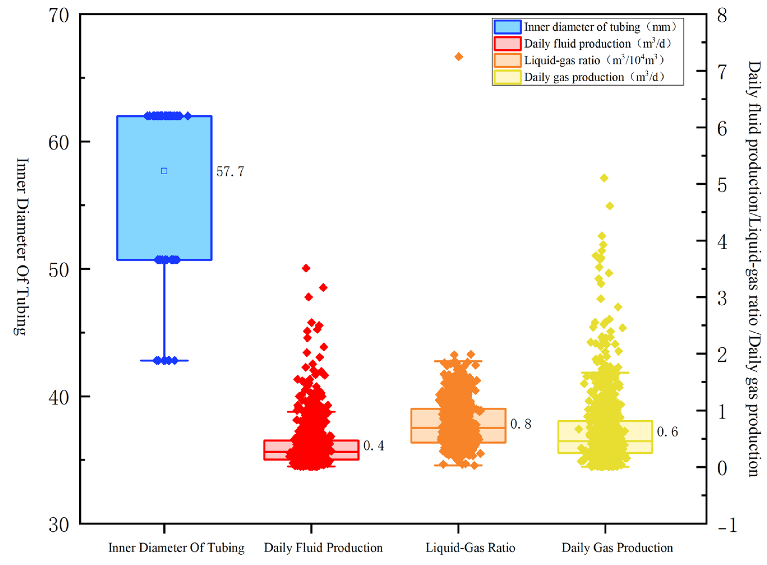
Based on the actual field data of gas wells in a tight gas reservoir in the Ordos Basin, a boxplot statistical analysis (Figure 1) was conducted to determine the value ranges of key parameters such as tubing inner diameter, liquid–gas ratio, liquid production rate, and gas production rate. These ranges were then used as the basis for setting the experimental parameters, as shown in Table 2.
A total of 33 experimental cases were designed and conducted across the four flow patterns. Rather than relying on a number of randomly distributed data points, the experimental matrix was strategically configured to ensure comprehensive coverage of the transition boundaries for each flow pattern. Specifically, the gas production rate was systematically varied from 0.25 to 2.5 × 10⁴ m3/d, covering the full range from bubbly flow (≤0.012 × 10⁴ m3/d) through slug flow (0.012–0.2 × 10⁴ m3/d) and churn flow (0.2–0.37 × 10⁴ m3/d) to annular flow (≥0.37 × 10⁴ m3/d). This stratified experimental design ensures that each flow pattern is adequately represented, with multiple replicates at different operating conditions to capture the intra-pattern variability. For each operating condition, measurements were repeated three times and the arithmetic mean was adopted as the steady-state value, thereby enhancing data reliability. The 33 cases thus constitute a representative and purposefully designed dataset that reflects the actual operating envelope of tight gas wells in the Ordos Basin, rather than an arbitrary collection of experimental runs.

2.2. Experimental Procedure

The main experimental procedure is as follows:
(1)
System startup and gas flow rate regulation: Open the air inlet valve of the storage tank and the air compressor, start the data acquisition system (sampling frequency: 1 Hz), and record the initial environmental parameters. Adjust the pneumatic valve so that the gas flow rate stabilizes within ±2% of the target value. After maintaining stability for 2 min, record the reading of the gas flowmeter.
(2)
Liquid flow rate regulation and two-phase mixing: Open the outlet valve of the liquid storage tank, start the liquid flowmeter, and then adjust the liquid branch valve to set the liquid flow rate to the desired values (0.5, 1.0, 1.5 m3/d). After the gas and liquid phases are thoroughly mixed in the mixer and enter the vertical test section, observe the flow state in the section and wait for the flow parameters (pressure, temperature, and flow rate) to stabilize (stability criterion: fluctuations of each parameter within ±1% of the set value over 2 min).
(3)
Flow pattern imaging and data acquisition: Once stabilized, activate the high-speed camera to capture gas–liquid flow pattern images through the transparent window of the test section. Annotate the operating condition number, time, pipe diameter, and inclination angle, and preliminarily determine the flow pattern type based on the visual images. Simultaneously, continuously acquire pressure, temperature, differential pressure, and flow rate data for 3 min, and take the arithmetic mean values as the steady-state values for that operating condition.
(4)
Liquid holdup measurement (quick-closing valve method): Immediately after completing data acquisition for each steady-state condition, perform liquid holdup measurement. A set of pneumatic quick-closing valves (response time < 0.1 s) is installed upstream and downstream of the test section. While keeping the gas and liquid flow rates unchanged, trigger both quick-closing valves to close simultaneously, trapping the gas–liquid mixture in the test section of known length. Then open the drain valve to discharge the trapped liquid into a measuring cylinder, read the liquid volume, and calculate the average liquid holdup based on the inner diameter and length of the test section. Repeat the measurement three times for each condition and take the average value as the experimental liquid holdup for that flow pattern. After measurement, reopen the quick-closing valves to resume flow, and wait for stabilization before adjusting the flow rates for the next set of conditions.
(5)
Repetition of the same condition and traversing multiple conditions: After completing one set of conditions, first adjust the liquid flow rate to the next set value and allow stabilization, then fine-tune the pneumatic valve to calibrate the gas flow rate. Repeat steps (2)–(4) to complete all preset liquid–gas ratio tests under the same pipe diameter and inclination angle. Thereafter, change the pipe diameter (40, 60, or 75 mm) or adjust the inclination angle (0–90°), and repeat the above procedures of gas/liquid regulation, data acquisition, and liquid holdup measurement.
(6)
Experiment termination and system cleaning: After all test conditions are completed, close the liquid valve, gas valve, pneumatic valves, and compressor in sequence, and slowly release the storage tank pressure to atmospheric pressure. Turn on dry air purging to remove residual liquid from the test section. Turn off all power supplies, organize the experimental data, and clean the bench.
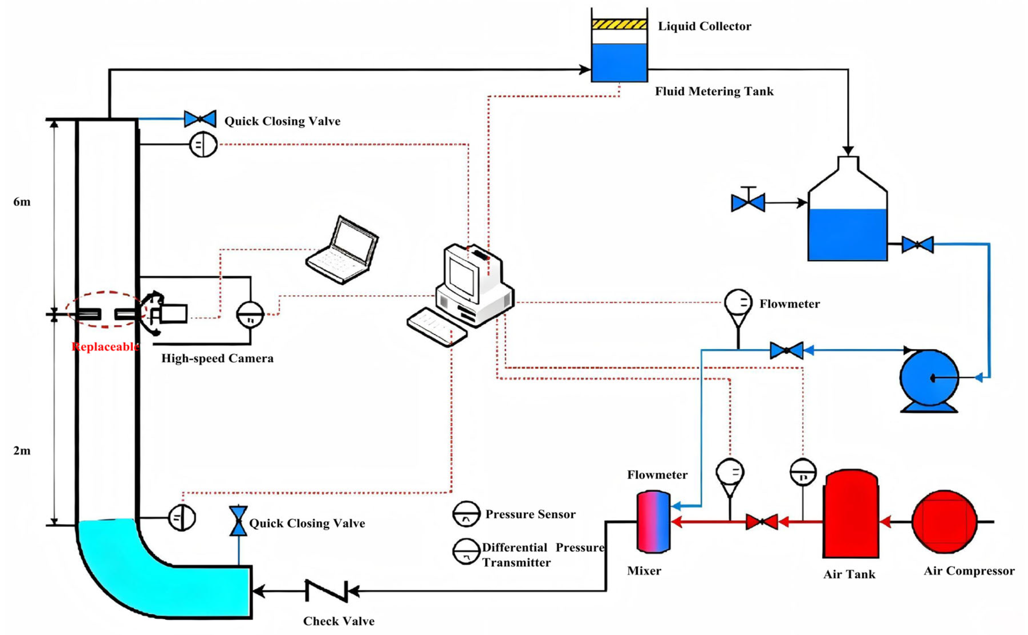
Throughout the entire experimental procedure, gas and liquid flow rates, pressure, temperature, and differential pressure data are automatically recorded by the data acquisition system, while flow pattern images and liquid holdup measurements are manually recorded and cross-validated to ensure the reliability and reproducibility of the experimental results. A schematic diagram of the gas–liquid two-phase flow loop is shown in Figure 2.

2.3. Experimental Uncertainty Analysis

To ensure the reliability of the experimental data, a comprehensive uncertainty analysis was conducted on the experimental setup. The measurement accuracies of all sensors are summarized in Table 1. The pressure sensor has an accuracy of ±0.1% within the range of 0–3.5 MPa, and the differential pressure measurements are derived from the difference between two pressure sensors. Based on the standard error propagation method using the sensor accuracies listed in Table 1, the combined uncertainty for the pressure drop is estimated to be ±3.2%.
Regarding repeatability, each experimental condition was measured three times, as described in the experimental procedure. The relative standard deviation (RSD) of the pressure drop measurements, calculated from the three repeated measurements for each condition, is within ±2.5% across all cases, indicating satisfactory measurement reproducibility.
For liquid holdup measurements using the quick-closing valve method, the primary sources of uncertainty include the volume reading error of the graduated cylinder (±1 mL) and the determination of the test section volume (±0.5%). The combined uncertainty for liquid holdup is estimated to be ±2.8%.
The influence of measurement errors on the model coefficients was inherently accounted for by the PSO algorithm, as its objective function is constructed upon the discrepancy between measured and predicted values. In subsequent studies, the provided optimization correction coefficients are considered robust within the observed experimental uncertainty range.

2.4. Analysis of Experimental Results

2.4.1. Analysis of Experimental Flow Patterns

To physically simulate the flow behavior in actual gas wells, a segmented simulation approach was adopted. In a gas well, the gas–liquid flow velocity gradually increases from the bottomhole to the wellhead, reaching its maximum at the wellhead. The wellbore was thus divided into multiple segments along this path. By progressively increasing the gas flow rate from low to high, the entire process of flow velocity rising from low to high along the bottomhole-to-wellhead direction was effectively reproduced. Using this method, four typical vertical wellbore flow patterns—bubbly flow, slug flow, churn flow, and annular flow—were successfully generated, and their transition boundaries were determined (Table 3).

2.4.2. Analysis of Liquid Holdup Results

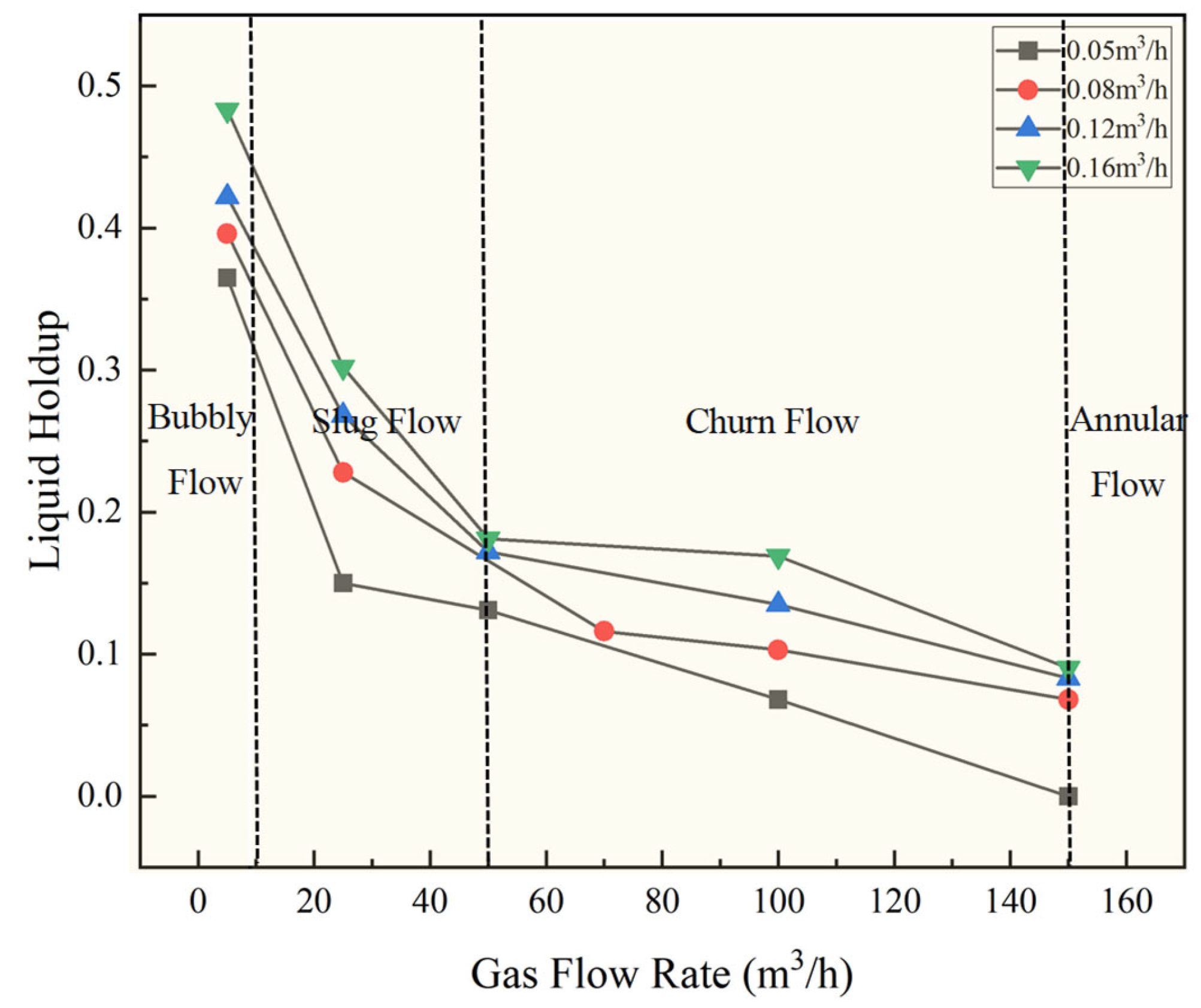
Figure 3 illustrates the variation in liquid holdup with gas flow rate. At a constant liquid flow rate, the liquid holdup decreases continuously as the gas flow rate increases. At a constant gas flow rate, the liquid holdup increases with increasing liquid flow rate. In the high gas flow rate region, the downward trend of the curve becomes gentler, and the liquid holdup tends to approach a stable value, corresponding to a flow pattern transition from churn–slug flow to annular flow.
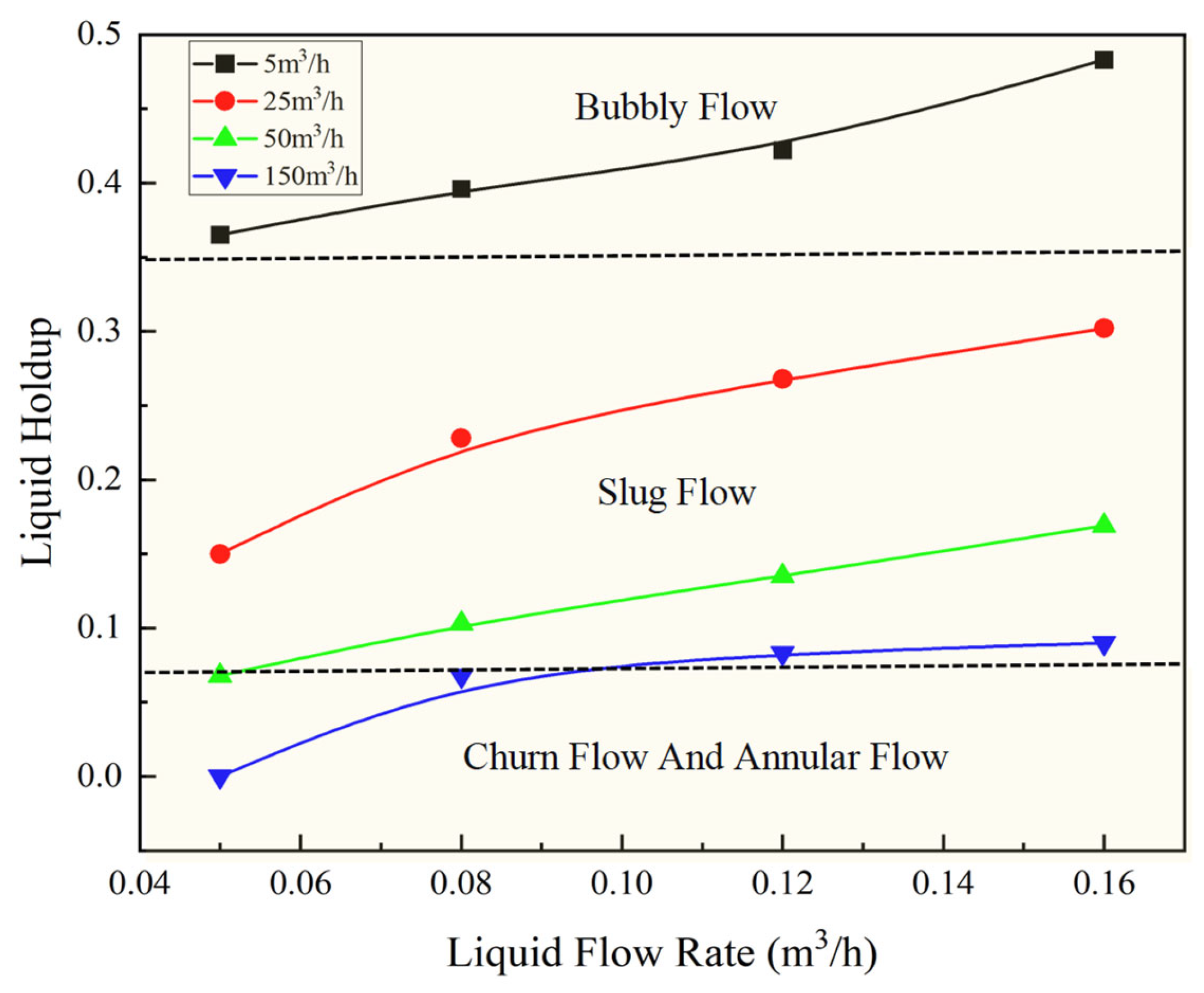
Figure 4 presents the variation in liquid holdup with liquid flow rate. At a given liquid flow rate, a higher gas flow rate corresponds to a lower liquid holdup. At a given gas flow rate, the liquid holdup tends to increase with rising liquid flow rate. Specifically, when the gas flow rate is below 5 m3/h, bubbly flow predominates; in the range of 25–50 m3/h, slug flow is dominant; and at gas flow rates exceeding 50 m3/h, the flow patterns are mainly churn flow and annular flow.

2.4.3. Analysis of Pressure Drop Results

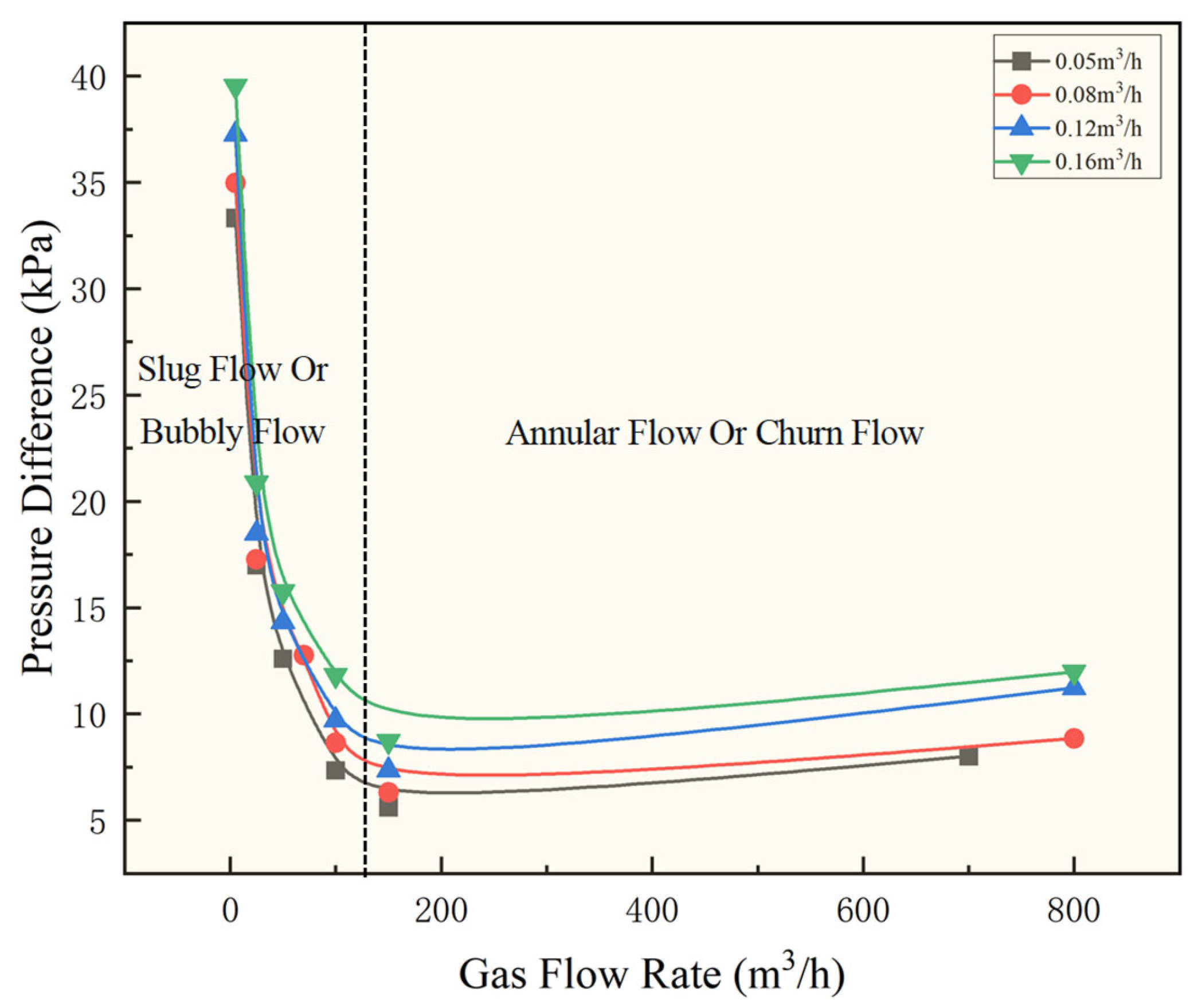
Figure 5 shows the variation in pressure drop with gas flow rate. At a given gas flow rate, the pressure drop increases with increasing liquid flow rate. At a given liquid flow rate, the pressure drop exhibits a distinct maximum as the gas flow rate increases, following an initial decrease and a subsequent increase. This maximum value increases with the liquid flow rate and corresponds to slug or bubbly flow. Beyond this maximum, the flow pattern gradually transitions to annular or churn flow.
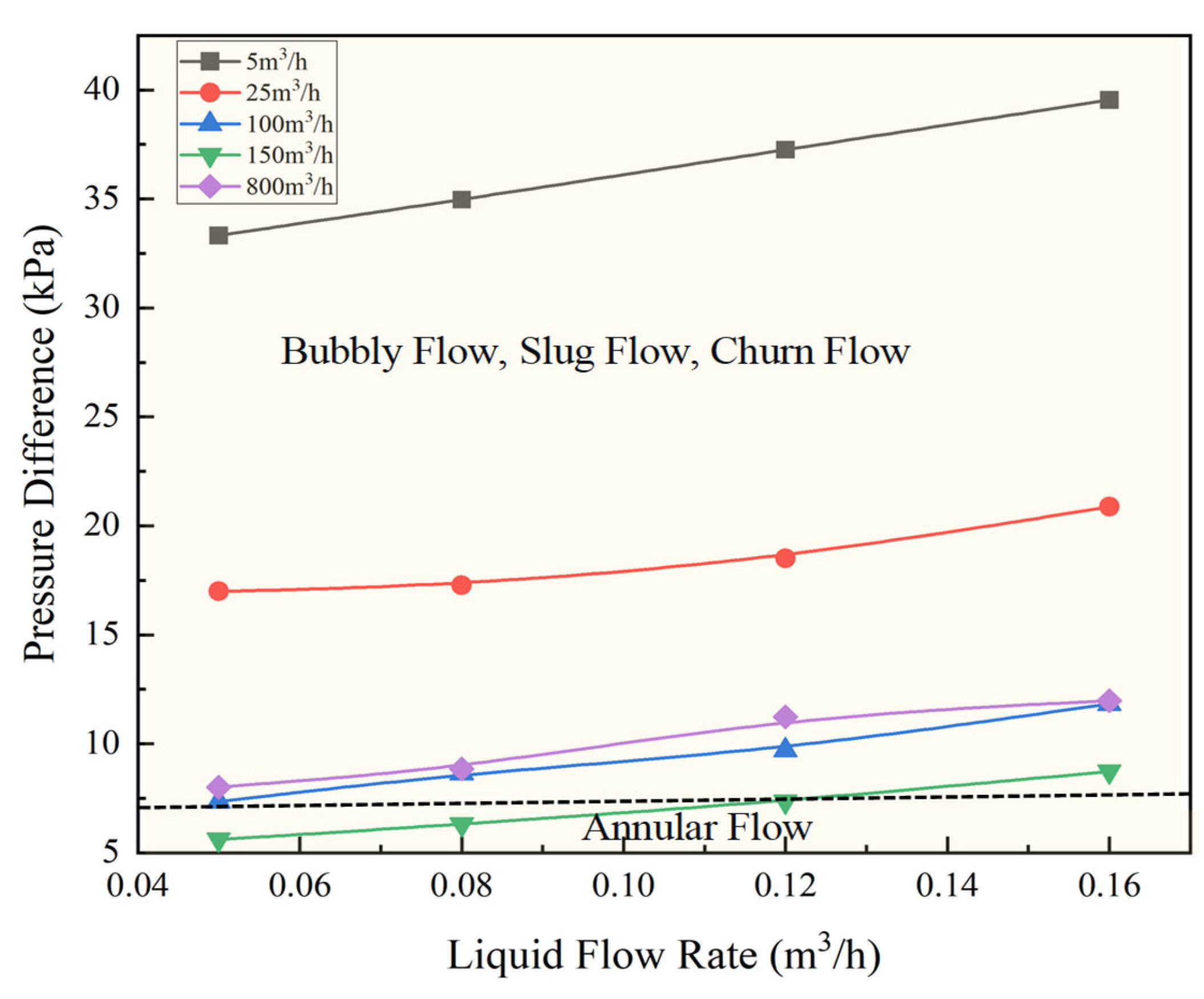
Figure 6 illustrates the variation in pressure drop with liquid flow rate. At a constant gas flow rate, the pressure drop increases with liquid flow rate. At a constant liquid flow rate, when the gas flow rate ranges between 5 and 150 m3/h, the pressure drop gradually decreases with increasing gas flow rate, and the flow patterns successively appear as bubbly flow, slug flow, and churn flow. When the gas flow rate exceeds 150 m3/h, the pressure drop gradually increases with gas flow rate, and the flow pattern is predominantly annular flow.

3. Model Selection for Flow Pattern Discrimination of Gas–Liquid Two-Phase Flow in Vertical Wellbores

Among the widely recognized methods for predicting gas–liquid flow patterns in vertical wellbores are the Ansari, Beggs–Brill, Mukherjee–Brill, and Aziz models. Each model employs a consistent approach: transition boundaries between different flow patterns are established based on extensive experimental data, and corresponding flow pattern maps are then constructed. The Aziz model is taken here as an example to illustrate how such a flow pattern map is specifically derived.
First, the dimensionless gas superficial velocity N x and liquid superficial velocity, N y are calculated using Equations (1) and (2):
N x = 3.28 v s g ρ g ρ a 1 / 8 ρ l σ w ρ w σ 1 / 4
N y = 3.28 v s l ( ρ l σ w ρ w σ ) 1 4
where v s g is the gas superficial velocity (m/s); v s l is the liquid superficial velocity (m/s); ρ g is the density of the gas phase under flowing conditions (kg/ m3); ρ l is the density of the liquid phase under flowing conditions (kg/m3); ρ a is the density of air under standard conditions (kg/m3); ρ w is the density of water under standard conditions (kg/m3); σ is the surface tension of the liquid phase under flowing conditions (mN/m); σ w is the surface tension of water under standard conditions (mN/m).
Next, the transition boundaries between different flow patterns are determined using Equations (3)–(5):
N 1 = 0.51 ( 100 N y ) 0.172
N 2 = 8.6 + 3.8 N y ,
N 3 = 70 ( 100 N y ) 0.152
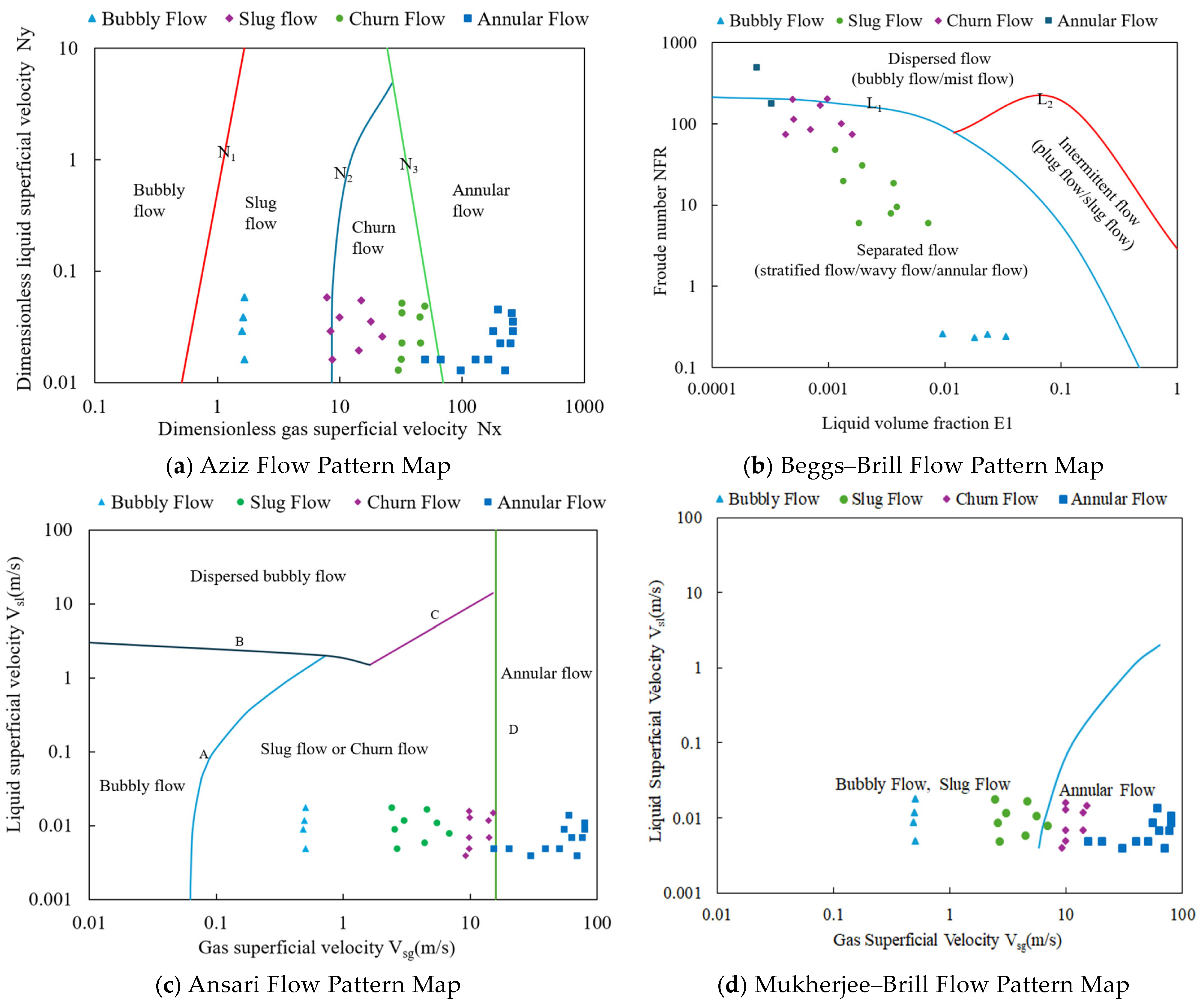
Finally, using the calculated dimensionless gas superficial velocity N x and liquid superficial velocity N y , the data points are plotted on the Aziz flow pattern map, as shown in Figure 7a. Following the same procedure, the flow pattern maps for the Ansari, Beggs–Brill, and Mukherjee–Brill models are constructed based on their respective transition boundaries, as presented in Figure 7b–d.
As shown in Figure 7, discrepancies exist among the different correlations in flow pattern prediction. A comparison of the experimental data with the various flow pattern maps indicates that the Aziz, Mukherjee–Brill, and Ansari models yield higher prediction accuracy, whereas the Beggs–Brill model exhibits the most pronounced deviations. However, the Mukherjee–Brill model can only identify the transition boundaries between bubbly flow and slug flow, and between slug flow and annular flow, while the Ansari model fails to accurately distinguish slug flow from churn flow. In contrast, the Aziz model not only covers all four flow patterns—bubbly, slug, churn, and annular—but also allows for subsequent correction of the liquid holdup coefficients and friction factor coefficients for each pattern. Therefore, the Aziz model is selected as the optimal flow pattern identification model for this study.

4. Correction and Optimization of Pressure Drop Prediction Models for Vertical Wellbores

Under the current experimental conditions, the flow patterns observed are bubbly flow, slug flow, churn flow, and annular flow. Accordingly, based on the selected optimal flow pattern identification model above, the pressure drop calculation methods for each of the four flow patterns are presented as follows.
The total pressure gradient comprises the gravitational, frictional, and acceleration pressure gradients, as given by Equation (6):
d p d z = d p d z h + d p d z f r + d p d z a
where d p d z is the total pressure gradient, d p d z h is the gravitational pressure gradient, P a / m ; d p d z f r is the frictional pressure gradient, P a / m ; d p d z a is the acceleration pressure gradient, P a / m .
Among these, the magnitude of the acceleration pressure gradient is very small and can be neglected.

4.1. Calculation Methods of Pressure Drop for Different Flow Patterns

(1)
For bubbly flow, Aziz et al. (1972) [6] proposed the pressure drop formula given by Equation (7):
d p d z = ρ m g sin θ + λ ρ m ν m 2 2 D
ρ m = ρ l H l + ρ g ( 1 H l )
v m = v s l + v s g
where ρ m is the average density of the gas–liquid mixture, kg/m3; λ is the friction factor, dimensionless; v m is the average velocity of the gas–liquid mixture, m/s; v s l is the liquid superficial velocity, m/s; v s g is the gas superficial velocity, m/s; θ is the wellbore inclination angle; D is the tubing diameter; H l is the liquid holdup.
(2)
For slug flow, Aziz et al. proposed the pressure drop formula given by Equation (10).
( d p d z ) s = ρ m g sin θ + λ ρ l H l ν m 2 2 D
(3)
For annular flow, the Duns Ros [27] method should be adopted for calculation according to Region III, as shown in Equation (11).
( d p d z ) c m = 2 f R ν s g 2 ρ g D ( 1 + ν s l ν s g )
where f R is the Ros resistance coefficient, dimensionless.
(4)
For churn flow, the pressure gradient must be calculated using a linear weighting of the formulas for slug flow and annular flow simultaneously, as shown in Equation (12).
d p d z = A ( d p d z ) S + B ( d p d z ) c m
Additionally,
A = N 3 N x N 3 N 2 , B = 1 A
where N 2 , N 3 , N x are all dimensionless gas/liquid superficial velocities.
Using the above calculation methods for each flow pattern in the original Aziz model, the predicted pressure drop can be obtained. However, the calculated pressure drop deviates significantly from the measured values, as will be discussed in the subsequent study. Given that the liquid holdup coefficient is the core parameter governing the gravitational pressure drop, while the frictional pressure drop is governed by the friction factor, it is necessary to correct both the liquid holdup coefficient and the friction factor in the original model to improve its pressure drop prediction accuracy.

4.2. Correction of the Pressure Drop Prediction Model for Vertical Wellbores

Based on the optimally selected Aziz model described above, it is necessary to correct the liquid holdup coefficient α 1 in the gravitational pressure drop and the friction coefficient α 2 in the frictional pressure drop. Since the Aziz model introduces coefficients A and B for churn flow, which are difficult to correct using traditional methods, an intelligent optimization algorithm is adopted for model calibration in this study. The corrected formulas are shown in Equations (16)–(19). The specific correction process is as follows.

4.2.1. Principle of Particle Swarm Optimization Algorithm

The Particle Swarm Optimization (PSO) algorithm was originally developed in the 1990s by Eberhart and Kennedy, based on the study of bird flock foraging behavior. In simple terms, PSO utilizes individuals within a population to share and transmit information. Through the combination of each individual information and the shared information within the population, the swarm moves in a directional manner within the target problem space to search for the optimal solution.
The entire iterative process of PSO is analogous to a bird flock searching for food, where the location of the food represents the position of the optimal solution. During the foraging process of birds, the initial positions of all individuals in the flock are randomly distributed. The swarm aims to locate the global optimum, whose position is unknown a priori. Birds can only adjust their searching direction through information exchange among themselves and their own perception of the food location, ultimately finding the food (optimal solution). In this model, each bird can be regarded as a particle. Assuming there are M particles in a D-dimensional space, the position of the best food source perceived by the entire population is denoted as gbest, while the best position perceived by each individual particle is denoted as pbest. The mathematical representation can be expressed as follows:
V i d ( t + 1 ) = w v i d ( t ) + c 1 r 1 ( g best d ( t ) x i d ( t ) ) + c 2 r 2 ( p best d ( t ) x i d ( t ) )
x i d ( t + 1 ) = x i d ( t ) + α v i d ( t + 1 )
where w is the inertia weight that controls the velocity weighting of particles and adjusts the search scope within the solution space; c 1 and c 2 are acceleration constants that regulate the maximum learning step size of particles; γ 1 and γ 2 are two random numbers in the range [0, 1] that increase the randomness of the search; α is a constriction factor used to control the velocity weighting; x ( t ) and v ( t ) denote the current position and velocity of particle, respectively; x ( t + 1 ) and v ( t + 1 ) represent the position and velocity of the particle in the next iteration. One of the distinctive features of the particle swarm optimization algorithm is its memory capability, which allows particles to learn from one another within the swarm.

4.2.2. Model Calibration Using Particle Swarm Optimization

Based on the principle of the particle swarm optimization algorithm described above, the pressure drop prediction model was calibrated, and the calibrated formulas are given in Equations (16)–(19). The specific calibration procedure is as follows:
(1)
The calculation formula for bubbly flow is shown in Equation (16).
( Δ p Δ z ) b = [ α 2 λ [ ρ l α 1 H l + ρ g ( 1 α 1 H l ) v m 2 ] 2 D ] + [ ρ l α 1 H l + ρ g ( 1 α 1 H l ) ] * g sin θ ] * Δ z
(2)
The calculation formula for slug flow is shown in Equation (17).
( Δ p l Δ z ) s = [ α 2 λ ρ l α 1 H l v m 2 2 D + [ ρ l α 1 H l + ρ g ( 1 α 1 H l ) ] * g sin θ ] * Δ z
(3)
The calculation formula for churn flow is shown in Equation (18).
( Δ p Δ z ) a = ( β 1 A ) ( Δ p Δ z ) s + ( β 2 B ) ( Δ p Δ z ) C M
(4)
The calculation formula for annular flow is shown in Equation (19).
( Δ p Δ z ) c m = [ α 2 2 f R v s g 2 ρ g D ( 1 + v s l v s g ) + [ ρ l α 1 H l + ρ g ( 1 α 1 H l ) ] g sin θ ] * Δ z
Based on the ratio of the measured liquid holdup H l m to the calculated liquid holdup H l c from eight sets of slug flow experimental data, the correction coefficient α 1 for liquid holdup can be obtained. The specific procedure for calculating the liquid holdup is shown in Equations (20)–(22).
v b s = 1.41 [ σ g ( ρ l ρ g ) ρ l 2 ] 1 4
v b f = 1.2 v m + v b s
H l c = 1 v s g v s l
where v b f is the rising velocity of bubbles in the liquid flow, m/s; v b s is the rising velocity of bubbles in a stationary liquid, m/s; g is the gravitational acceleration, m/s2.
The correction coefficient α 1 needs to take the average value of 8 groups of experiments to ensure its accuracy, as shown in Equation (23).
α 1 = 1 n i = 1 n ( H l m H l c ) = 0.825
The correction method for the frictional factor correction coefficient α 2 is similar to that for the liquid holdup correction coefficient α 1 . However, since the frictional factor coefficient cannot be measured experimentally, it is first necessary to calculate the frictional pressure drop from the experiment. The specific procedure for calculating the frictional factor coefficient is given in Equations (24)–(27).
Δ p E f r = Δ p E Δ p G
λ E = Δ p E f r × 2 D ρ m v m 2 Δ Z
λ C = λ E λ calculation
α 2 = i = 1 n λ i C Δ p i E f r i = 1 n Δ p i E f r = 1.77
where Δ p E f r is the frictional factor pressure drop measured from the experiment, Δ p E represents experiment, Δ p G is the gravitational pressure drop, λ c alculation can be obtained from the Moody chart [28].
Based on the above method, the liquid holdup correction coefficient and the frictional factor correction coefficient for each flow pattern are calculated, as shown in Table 4. According to Equation (12), the correction for churn flow is related to the correction coefficient α 1 , α 2 of slug flow and annular flow, as presented in Table 4.
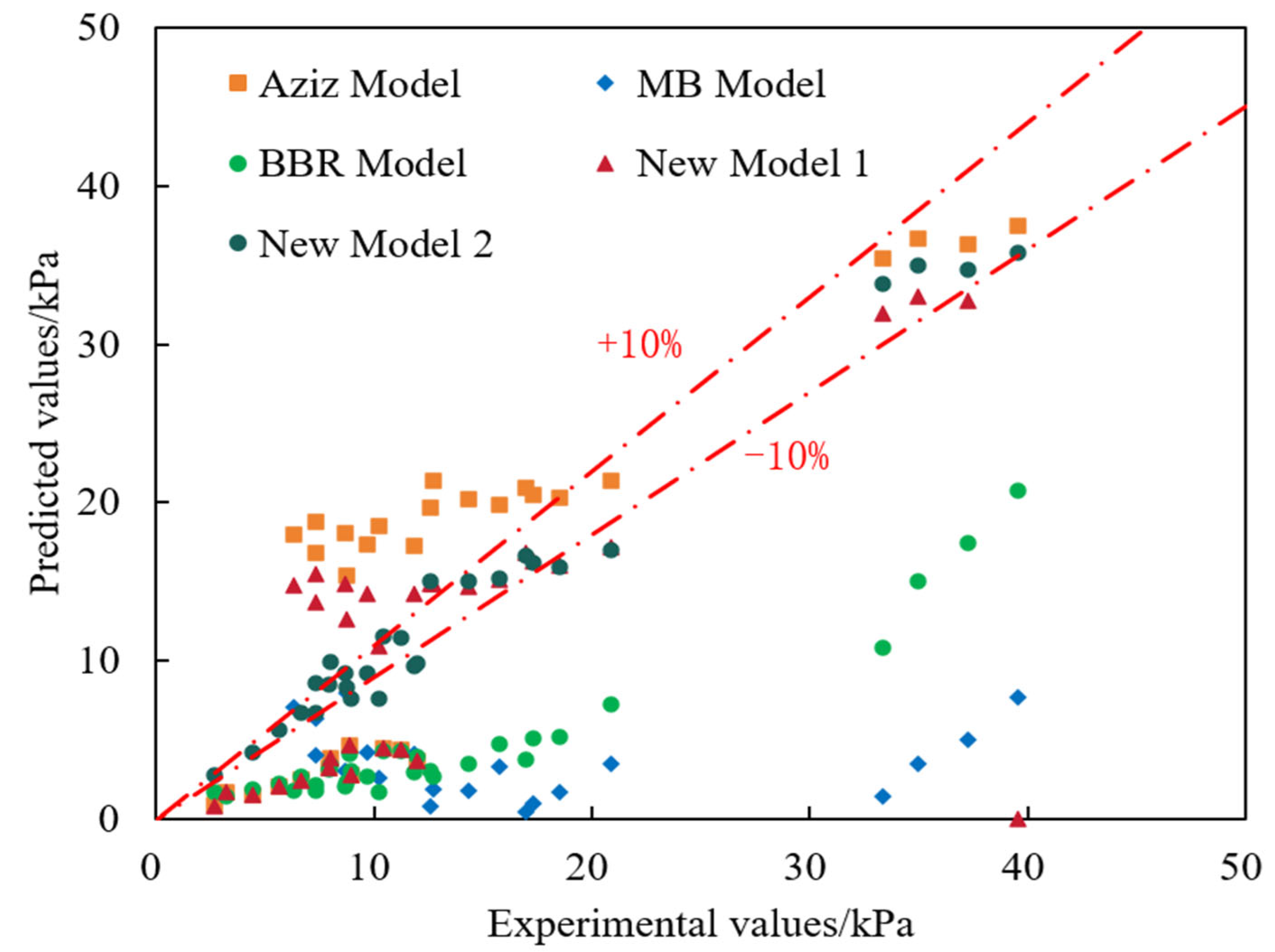
The error of the new model (Model 1) obtained through the above manual calculations and correction process remains relatively large, as shown in Figure 8 and Section 4.3. Since Model 1 only compares errors through manual calculations, it is difficult to effectively correct the coefficients A and B in the churn flow. Therefore, this study abandons the traditional concept of average correction and adopts the Particle Swarm Optimization (PSO) algorithm, a swarm intelligence method, to perform corrections with the objective of minimizing the comprehensive error of each experimental group. The liquid holdup correction coefficient α 1 , the frictional factor correction coefficient α 2 , and the correction coefficients β 1 and β 2 for A and B in the formula have been recalculated. The correction coefficients for the new model (Model 2) are obtained, as shown in Table 5.
The PSO algorithm was configured with the following parameters: a population size of 80, a maximum number of iterations of 3000, an inertia weight ω linearly decreasing from 0.9 to 0.4 during the iterations, and acceleration constants c 1 = c 2 = 2.0 . The search ranges for the correction coefficients were set as: C H 0 , 2 for liquid holdup, C F 0 , 5 for friction factor, and for the churn flow A 0.5 , 2.0 , B 0.1 , 1.0 . These ranges were determined based on preliminary sensitivity tests to ensure adequate coverage of the feasible parameter space while maintaining computational efficiency.
Where C H is the correction coefficient for liquid holdup (dimensionless), and C F is the correction coefficient for friction factor (dimensionless).
It should be noted that the same 33 experimental cases were used for both the PSO and model assessment. To mitigate the risk of overfitting, the PSO algorithm was configured with a relatively small population size (80) and a sufficient number of iterations (3000) to ensure convergence without excessive tuning to the training data. More importantly, the optimization was constrained by the mechanistic structure of the Aziz model, which significantly reduces the degrees of freedom compared with purely data-driven approaches. The correction coefficients were optimized separately for each flow pattern, and the objective function was defined as the mean absolute percentage error (MAPE) across all cases. As demonstrated in Table 6 and Figure 8, the PSO-optimized Model 2 achieves consistent accuracy improvements across all four flow patterns, rather than excelling only on a subset of cases, which suggests that the model has not been overfitted to specific data points.
The optimized correction coefficients reflect distinct physical mechanisms across flow patterns. The liquid holdup correction coefficient is 0.96 (near unity) for bubbly flow, decreases to 0.84 for slug flow, and rises sharply to 4.79 for annular flow. For churn flow, the weighting coefficients (A = 1.2, B = 0.62) indicate pressure drop characteristics closer to slug flow, consistent with its transitional nature between the two regimes. These variations correspond to different dominant pressure drop mechanisms: gravitational pressure drop prevails in bubbly and slug flows, while frictional pressure drop dominates annular flow, with churn flow exhibiting transitional features. This validates the physical rationale of flow pattern-specific correction.

4.3. Evaluation of the Pressure Drop Prediction Model for Vertical Wellbores

Based on the gas–liquid two-phase physical experiments, a total of 33 sets of pressure drop data corresponding to the four flow patterns were obtained. Figure 8 compares the predicted values of different pressure drop prediction models with the experimental values. The models compared include Aziz, Beggs–Brill, Mukherjee–Brill, as well as the corrected Model 1 and Model 2. The results indicate that the traditional models (Aziz, Beggs–Brill, and Mukherjee–Brill) exhibit substantial pressure drop prediction errors, while the calculation error of the corrected Model 2 is further reduced compared to Model 1.
In this study, the Root Mean Square Error (RMSE) and the Mean Absolute Percentage Error (MAPE) are selected as model evaluation metrics. RMSE measures the deviation between the predicted and actual values, assigning greater weight to larger errors. MAPE expresses the relative error between the predicted and actual values as a percentage, placing greater emphasis on the magnitude of relative errors. For both metrics, smaller values indicate smaller errors and thus better model performance. Since the two metrics have different emphases, their combined use provides a more comprehensive evaluation of the model effectiveness. Table 6 presents a comparison of the RMSE and MAPE for each model. The calculation formulas for RMSE and MAPE are as follows:
R M S E = 1 n 1 n ( Δ P c a l Δ P c a p ) 2
M A P E = 1 n 1 n Δ P cal Δ P cap Δ P cap × 100 %
where Δ P c a l is the pressure difference predicted by the model; Δ P c a p is the pressure difference measured experimentally.
Based on the errors shown in Table 6, the new Model 2 proposed in this paper exhibits higher prediction accuracy under different flow pattern conditions: its Mean Absolute Percentage Error (MAPE) is 11.9%, and its Root Mean Square Error (RMSE) is 1.9 kPa. In comparison, the traditional empirical model Aziz has a MAPE of 50.6% and an RMSE of 5.3 kPa, while the manually corrected new Model 1 has a MAPE of 18.2% and an RMSE of 4.9 kPa. Both errors of new Model 2 are smaller than those of the above models, indicating that new Model 2 can predict pressure drop more accurately. Therefore, for the conversion of pressure drop under different flow patterns in tight gas wells, it is recommended to use the new Model 2 proposed in this study to calculate the pressure drop in a vertical wellbore. By combining the new Model 2 with the choke nozzle flow model, the conversion from wellhead tubing pressure to bottomhole flowing pressure in the vertical wellbore of a gas well with a choke can be accomplished.
In recent years, machine learning (ML) methods have also been applied to predict two-phase flow pressure drop with promising results. For instance, Li (2024) [17] developed a neural network-based model for liquid holdup and pressure drop prediction, and Liu et al. (2025) [18] proposed an ML-assisted correlation for annular flow pressure drop. These data-driven methods can achieve high accuracy but typically require large datasets and lack physical interpretability. In contrast, the model proposed in this study retains the mechanistic structure of the Aziz model and only employs PSO to optimize the key coefficients, representing a mechanism-intelligent combined method that achieves both high prediction accuracy and good physical interpretability.

4.4. New Model 2 Validation

To rigorously evaluate the predictive capability of the proposed Model 2, four additional independent experimental cases were conducted. As summarized in Table 7, the relative errors between the predicted and experimental pressure drops are 4.2% for bubbly flow, 11.7% for slug flow, 15.7% for churn flow, and 16.4% for annular flow, with an overall average MAPE of 12.0%. The prediction error of the independent validation set is close to that of the calibration dataset, which verifies that the model has good generalization performance without overfitting. This confirms that Model 2 maintains satisfactory prediction accuracy under various flow pattern conditions.
In terms of applicability, Model 2 is calibrated based on experimental data of vertical wellbores with a tubing inner diameter of 60 mm, a working pressure range of 0–3.5 MPa, and a liquid–gas ratio range of 0.4–4.0 m3/104 m3, and a gas–water two-phase fluid, which is mainly applicable to pressure drop calculation of vertical wellbores in tight gas reservoirs with low liquid–gas ratio characteristics. When the application scenarios deviate significantly from the above ranges (such as highly deviated wellbores, heavy oil systems, ultra-high pressure conditions), it is recommended to recalibrate the correction coefficients based on local experimental or field data to ensure calculation accuracy.

5. Conclusions

In this study, physical experiments of gas–liquid two-phase flow in a vertical wellbore were systematically conducted, and comparative analysis as well as optimization and calibration of classic pressure drop prediction models were performed. The main conclusions are as follows:
(1)
Through segmented simulation of the gas flow velocity variation from the bottomhole to the wellhead, the four typical flow patterns—bubbly flow, slug flow, churn flow, and annular flow—were clearly observed and recorded on the experimental platform. The transition boundaries among these flow patterns were determined based on daily gas production rate, gas velocity, liquid holdup, and liquid–gas ratio, providing a reliable data foundation for flow pattern identification and model validation.
(2)
A comparison of four classical flow pattern identification models—Aziz, Beggs–Brill, Mukherjee–Brill, and Ansari—revealed that the Aziz model provides the most complete coverage of all four flow patterns and exhibits the highest consistency between predicted results and experimental observations. Therefore, it can be recommended as the preferred model for flow pattern identification in vertical wellbores.
(3)
To address the substantial pressure drop prediction errors of the original Aziz model, we calibrated the liquid holdup and friction factor using experimental data. Furthermore, the particle swarm optimization (PSO) algorithm was employed for optimal fitting, with the correction coefficients systematically adjusted to minimize the global error. A new pressure drop prediction model (referred to as Model 2) applicable to different flow patterns was thereby established. This model significantly improves the prediction accuracy, achieving an overall MAPE of 11.9% and an RMSE of 1.9 kPa. Model 2 yields an average MAPE of 12.0% on the independent validation dataset, maintaining satisfactory accuracy beyond the parameter calibration set. Compared with the classical Aziz model (MAPE of 50.6%, RMSE of 5.3 kPa) and the manually calibrated Model 1 (MAPE of 18.2%, RMSE of 4.9 kPa), the proposed model demonstrates a considerable improvement in prediction accuracy.
It should be noted that the current independent validation dataset only includes four cases (one for each flow pattern), and the scale of validation samples is relatively limited. Future work will further expand the experimental conditions and field production data to conduct large-scale validation of the model under broader operating parameters, so as to further improve the robustness and universality of the model.

Author Contributions

Conceptualization, W.X. and P.L.; Methodology, W.X. and S.D.; Validation, L.L. and C.Q.; Software, L.Z.; Investigation, L.L. and M.S.; Data curation, Y.W.; Writing—review and editing, W.X., S.D. and C.Q.; Supervision, W.X. and S.D.; Project administration, W.X. and P.L. All authors have read and agreed to the published version of the manuscript.

Funding

This research was jointly funded by the Major Science and Technology Project of Petro-China Company Limited, “Research on optimization of well pattern and fracture network and enhanced oil recovery technologies in developed oilfields”, grant number 2023ZZ25YJ02. The APC was funded by the above-mentioned funder.

Data Availability Statement

The original contributions presented in this study are included in the article. Further inquiries can be directed to the corresponding author.

Conflicts of Interest

Authors Wen Xu, Peng Li, Yunfan Wen, Lili Liu, Lian Zhao, and Mingyue Sui were employed by the company PetroChina Changqing Oilfield Company. The remaining authors (Chuanchao Qu and Shuaiwei Ding) declare that the research was conducted in the absence of any commercial or financial relationships that could be construed as a potential conflict of interest. The authors declare that this study received funding from PetroChina Company Limited. The funder was not involved in the study design, collection, analysis, interpretation of data, writing of this article or the decision to submit it for publication.

References

  1. Zhang, L. Application of bottom hole pressure calculation method for gas well with downhole throttling. J. Chengde Pet. Coll. 2022, 24, 34–39. [Google Scholar] [CrossRef]
  2. Liu, S.; Wang, H.; Luo, Y.; Wang, D.; Hu, Y.; Zhu, Z. A new method for determining the bottom hole pressure of downhole throttled gas wells. J. Xi’an Shiyou Univ. (Nat. Sci. Ed.) 2012, 27, 53–56. [Google Scholar] [CrossRef]
  3. Wang, H.; Yi, X.; Lu, Y. Status of research on vertical conduit flow of gas-liquid two phases in wellbore. Xinjiang Pet. Geol. 2006, 27, 740–742. [Google Scholar] [CrossRef]
  4. Liu, X.; Xu, Y.; Peng, H.; Mu, Q.; Cui, K.; Cao, X. Mechanistic modeling of two-phase flow in deviated wells. Oil Drill. Prod. Technol. 2009, 31, 52–57. [Google Scholar] [CrossRef]
  5. Li, S. Natural Gas Engineering; Petroleum Industry Press: Beijing, China, 2000. [Google Scholar]
  6. Aziz, K.; Govier, G.W. Pressure drop in wells producing oil and gas. J. Can. Pet. Technol. 1972, 11, 38–48. [Google Scholar] [CrossRef] [Scilit]
  7. Beggs, D.H.; Brill, J.P. A Study of two-phase flow in Inclined pipes. J. Pet. Technol. 1973, 25, 607–617. [Google Scholar] [CrossRef] [Scilit]
  8. Mukherjee, J. Pressure drop correlations for inclined two-phase flow. J. Energy Resour. Technol. 1985, 107, 549–554. [Google Scholar] [CrossRef] [Scilit]
  9. Ansari, A.; Sylvester, N.; Shoham, O. A comprehensive mechanistic model for upward two-phase flow in wellbores. Softw. Pract. Exp. 1994, 9, 143–151. [Google Scholar] [CrossRef]
  10. Chen, J. Pressure drop calculation for vertical flow of oil, gas, and water mixtures—Flow pattern-based calculation method. Pet. Explor. Dev. 1980, 7, 55–67. Available online: https://xuebao.nepu.edu.cn/info/1147/9643.htm (accessed on 24 June 2026). [CrossRef] [Scilit]
  11. Gao, S.; Liu, Y.; Zhang, Y.; Lai, X.; Li, S.; Luo, C.; Wang, W. The forecast and analysis of pressure of gas well of western sichuan gas field. J. Chongqing Univ. Sci. Technol. (Nat. Sci. Ed.) 2012, 14, 60–63. [Google Scholar] [CrossRef]
  12. Liu, T.; Wang, S.; Guo, X.; Pan, G.; Chen, H.; Wu, Z. New calculation method of gas-liquid two phase annular-mist flow pressure drop of wellbores in gas wells. Oil Drill. Prod. Technol. 2017, 39, 328–333. [Google Scholar] [CrossRef]
  13. Liu, Z.; Liao, R.; Lei, Y.; Wu, Z.; Zhao, Y. Pressure drop model of oil-gas two-phase flow in horizontal pipes with different diameters. Sci. Technol. Eng. 2019, 19, 137–143. [Google Scholar] [CrossRef]
  14. Liu, Y.; Bai, X.; Cheng, Y.; Wang, X.; Song, H.; Liang, R. Experimental study on pressure drop of gas-liquid two-phase flow in inclined annulus pipe. China Sci. Pap. 2020. [Google Scholar] [CrossRef]
  15. Cheng, Y.; Wu, H.; Chen, Y.; Liao, R. Experimental study on changing laws of pressure drop of gas liquid two phase flow in horizontal wells. China Energy Environ. Prot. 2019, 41, 68–72+116. [Google Scholar] [CrossRef]
  16. Wang, G. Study of Gas Wellbore Flow Dynamics in the Ma Xian Area. Master’s Thesis, Yangtze University, Jingzhou, China, 2023. [Google Scholar] [CrossRef]
  17. Li, L. Prediction of Liquid Holdup and Pressure Drop in Gas-Liquid Two-Phase Flow Based on Neural Network. Master’s Thesis, Yangtze University, Jingzhou, China, 2024. [Google Scholar] [CrossRef]
  18. Liu, Z.; Qian, X.; He, J.; Liao, R.; Chen, C. Pressure drop prediction model for vertically upward annular flow in annular space of oil tube and casing. Pet. Drill. Tech. 2025, 53, 16–125. [Google Scholar] [CrossRef]
  19. Lin, J.; Li, H.; Liu, Y.; Xu, S.; Liu, Y.; Cao, Y. Modeling studies on pressure gradient prediction for shale horizontal gas wells. Oil Field Equip. 2025, 54, 6–11. [Google Scholar] [CrossRef]
  20. Zeng, Q.; Hao, X.; Sui, T.; Xu, L.; Wang, Z.; Gao, W. Predictive method and its application of pressure drop in horizontal wellbore completion string with sliding sleeves. Spec. Oil Gas Reserv. 2024, 31, 159–165. [Google Scholar] [CrossRef]
  21. Osman, E.S.A. Artificial neural network models for identifying flow patterns and predicting liquid holdup in horizontal multiphase flow. SPE Prod. Facil. 2004, 19, 33–40. [Google Scholar] [CrossRef]
  22. Kanin, E.A.; Osiptsov, A.A.; Vainshtein, A.L.; Burnaev, E.V. A predictive model for steady-state multiphase pipe flow: Machine learning on lab data. J. Pet. Sci. Eng. 2019, 180, 727–746. [Google Scholar] [CrossRef] [Scilit]
  23. Ribeiro, J.X.F.; Liao, R.; Aliyu, A.M.; Yeung, H. Prediction of pressure gradient in two and three-phase flows in vertical pipes using an artificial neural network model. Int. J. Eng. Technol. Innov. 2019, 9, 155–170. [Google Scholar] [CrossRef] [Scilit]
  24. Chaari, M.; Ben Hmida, J.; Seibi, A.C.; Al-Abdeli, Y.M. An integrated genetic algorithm artificial neural network approach for steady-state modeling of two-phase pressure drop in pipes. SPE Prod. Oper. 2020, 35, 628–640. [Google Scholar] [CrossRef] [Scilit]
  25. Zhou, D.; Liao, R.; Wang, W.; Yang, Z. Optimization of the pressure drop prediction model of wellbore multiphase flow based on simultaneous perturbation stochastic approximation. Int. J. Heat Technol. 2022, 40, 1397–1403. [Google Scholar] [CrossRef] [Scilit]
  26. Faraji, F.; Santim, C.; Chong, P.L.; Parsi, M.; Kim, S. Two-phase flow pressure drop modelling in horizontal pipes with different diameters. Nucl. Eng. Des. 2022, 395, 111863. [Google Scholar] [CrossRef] [Scilit]
  27. Duns, H.; Ros, N. Vertical flow of gas and liquid mixtures in wells. In Proceedings of the 6th World Petroleum Congress, Frankfurt am Main, Germany, 19–26 June 1963. [Google Scholar]
  28. Chen, J. Oil-Gas Two-Phase Pipe Flow; Petroleum Industry Press: Beijing, China, 1989. [Google Scholar]
Figure 1. Box plot of experimental parameters.
Processes 14 02395 g001
Figure 2. Experimental setup and process.
Processes 14 02395 g002
Figure 3. Variation in liquid holdup with gas volume.
Processes 14 02395 g003
Figure 4. Variation in liquid holdup with liquid volume.
Processes 14 02395 g004
Figure 5. Relationship between pressure drop and gas volume variation.
Processes 14 02395 g005
Figure 6. Pattern of pressure drop variation with liquid volume.
Processes 14 02395 g006
Figure 7. Comparison of Flow Pattern Maps.
Processes 14 02395 g007
Figure 8. Comparison of predicted values and experimental values of different pressure drop models.
Processes 14 02395 g008
Table 1. Measurement range and accuracy of the experimental device.
EquipmentMeasurement RangeMeasurement Accuracy/%
Pressure Sensor0–3.5 MPa±0.1
Temperature Sensor0–90 °C±0.5
Liquid Flowmeter2–20 m3/h±0.3
Gas–liquid Flowmeter160–2000 m3/h±1
Table 2. Range of experimental parameters.
ParametersTubing Inner Diameter (mm)Liquid–Gas Ratio (m3/104 m3)Liquid Production Rate (m3/d)Gas Production Rate (104 m3)
Average620.770.390.6
Experimental values600.4–4.00.5–50.25–2.5
Table 3. Visualization of different flow patterns and their transition boundaries.
Bubbly Flow
Daily Gas Production Rate Boundary (104 m3/d): ≤0.012Processes 14 02395 i001
Flow Velocity Boundary (m/s): ≤1
Liquid–Gas Ratio Boundary (m3/104 m3): ≥100
Churn Flow
Daily Gas Production Rate Boundary (104 m3/d): 0.2~0.37Processes 14 02395 i002
Flow Velocity Boundary (m/s): 6~10
Liquid–Gas Ratio Boundary (m3/104 m3): 4~10
Slug Flow
Daily Gas Production Rate Boundary (104 m3/d): 0.012~0.2Processes 14 02395 i003
Flow Velocity Boundary (m/s): 1~6
Liquid–Gas Ratio Boundary (m3/104 m3): 10~100
Annular Flow
Daily Gas Production Rate Boundary (104 m3/d): ≥0.37Processes 14 02395 i004
Flow Velocity Boundary (m/s): ≥10
Liquid–Gas Ratio Boundary (m3/104 m3): ≤4
Table 4. Pressure Drop Correction Coefficients for Different Flow Patterns.
Flow PatternCorrection Coefficient
Liquid HoldupFrictional Factor
Bubbly Flow0.93.47
Slug Flow0.8251.77
Annular Flow01.84
Churn Flow0.825/01.77/1.84
Table 5. Pressure Drop Correction Coefficients for Different Flow Patterns.
Flow PatternCorrection Coefficient
Liquid HoldupFriction Factor β 1 β 2
Bubbly Flow0.960.74//
Slug Flow0.840.60//
Annular Flow4.792.57//
Churn Flow0.84/4.790.60/2.571.20.62
Table 6. Comparison of predicted values and experimental values of different pressure drop models.
Flow PatternModels
AzizMBBBRNew Model 1New Model 2
MAPE
(%)
RMSE
(kPa)
MAPE
(%)
RMSE
(kPa)
MAPE
(%)
RMSE
(kPa)
MAPE
(%)
RMSE
(kPa)
MAPE
(%)
RMSE
(kPa)
Bubbly Flow4.71.888.131.856.220.38.043.94.52.2
Slug Flow30.65.488.714.573.211.317.93.111.42.2
Annular Flow107.34.9156.6140.274.54.916.36.715.71.5
Churn Flow59.99.042.54.957.86.730.45.716.01.8
Average Error50.65.393.947.965.410.818.24.911.91.9
Table 7. Independent experimental validation of Model 2 for different flow patterns.
Flow PatternLiquid Flow Rate (m3/d)Gas Flow Rate (m3/d)Liquid–Gas Ratio (m3/104 m3)Measured Pressure Drop (kPa)Predicted Pressure Drop (kPa)MAPE (%)
Bubbly Flow3.13122255.738.139.74.2
Slug Flow3.26139923.320.422.811.7
Churn Flow2.8833048.711.413.215.7
Annular Flow2.1412,0571.86.77.816.4
Average Error/////12.0
Disclaimer/Publisher’s Note: The statements, opinions and data contained in all publications are solely those of the individual author(s) and contributor(s) and not of MDPI and/or the editor(s). MDPI and/or the editor(s) disclaim responsibility for any injury to people or property resulting from any ideas, methods, instructions or products referred to in the content.