Research on Predicting the Outflow and Sediment Process of the Middle Yellow Reservoirs Based on Deep Learning

Abstract

Accurate prediction of reservoir discharge and sediment load is essential for optimizing reservoir operations and mitigating downstream flood risks. In the middle reaches of the Yellow River, water–sediment evolution exhibits significant nonlinearity and temporal dependency. However, existing models often neglect the dynamic coupling between water–sediment evolution and storage–discharge states and lack hydrological prior constraints. To improve performance under complex conditions, this study developed models for the Sanmenxia and Xiaolangdi reservoirs based on historical hydrological data from 2002 to 2022, with features selected via Pearson correlation. By incorporating variables such as reservoir capacity, we evaluated four deep learning architectures: CNN, LSTM, CNN-LSTM, and TCN. Furthermore, a Genetic Algorithm (GA) was employed to optimize the hyperparameters, utilizing a custom fitness function that integrates Nash–Sutcliffe Efficiency (NSE) with non-negative boundary constraints to ensure the simultaneous optimization of predictive accuracy and hydrological consistency. Experimental results demonstrate that the CNN-LSTM model achieved superior performance. Specifically, the test set NSE values for discharge and sediment reached 0.927 and 0.821 for Sanmenxia, and 0.949 and 0.843 for Xiaolangdi, respectively. In outflow prediction, the feature weights of inflow and reservoir capacity for Sanmenxia exceed 45% and 35%, while for Xiaolangdi, those of upstream and local inflow exceed 40% and 55%, respectively. In sediment prediction, almost all feature weights exceed 15%. This research provides a valuable reference for intelligent reservoir management in the Yellow River, advancing deep learning applications in complex hydrological systems.

1. Introduction

To address the complex water–sediment issues in the middle reaches of the Yellow River while balancing comprehensive utilization goals such as water supply and power generation, key regulation and storage projects, including the Sanmenxia and Xiaolangdi reservoirs, have been constructed. These reservoirs play a pivotal role in flood control, sediment reduction, water resource allocation, and integrated basin management [1]. However, decades of progressive sediment accumulation have led to a substantial year-on-year decline in reservoir capacity, which significantly complicates reservoir operation and necessitates more scientific management strategies. In this context, the precise prediction of water–sediment processes—particularly outflow discharge and sediment concentration—serves as a critical prerequisite for optimized reservoir scheduling [2].

The dynamic variations in water–sediment processes in the middle reaches of the Yellow River are jointly influenced by multiple factors, including rainfall, upstream inflow, and reservoir operation, exhibiting significant nonlinearity and temporal dependency [3,4]. These characteristics pose substantial challenges to traditional prediction methods. Although deterministic physico-mathematical models and empirical statistical models can reflect water–sediment laws to some extent, they are highly dependent on input parameters and involve complex modeling processes, making them difficult to adapt to high-dimensional inputs and nonlinear system features [5,6,7,8]. To overcome these limitations, machine learning techniques have been progressively introduced. Algorithms such as Support Vector Machines (SVM), Random Forests (RF), and Gradient Boosting Decision Trees (GBDT) have improved the adaptive capacity and prediction accuracy of models to a certain degree [9,10,11,12]. Nevertheless, these models still face constraints when handling long-term dependencies and multi-dimensional temporal features.

In recent years, deep learning has been widely applied to water–sediment process prediction due to its outstanding ability to handle complex nonlinear problems. Fan et al. [13] developed a hybrid CNN-LSTM model integrated with wavelet transform, significantly enhancing the accuracy of sediment concentration prediction. Zhang et al. [14] introduced an attention mechanism to improve the multi-scale runoff prediction accuracy of CNN-LSTM models. Additionally, Ma et al. [15] validated the effectiveness of hybrid TCN-LSTM architectures in capturing complex hydrological dynamics, and Fan et al. [16] demonstrated that the VMD-MGGP-NGO-BiLSTM multi-stage optimization framework significantly boosts the forecasting precision of daily discharge and daily sediment concentration. Such hybrid integration is essential for capturing the complex, non-stationary dynamics that unitary models fail to resolve. Despite the generally high accuracy of these models, most rely on single hydrological time-series inputs and often neglect the dynamic relationship between water–sediment evolution and reservoir storage–discharge states. This leads to limited feature extraction dimensions and restricted generalization capabilities when facing complex operating conditions.

Furthermore, the performance of deep learning models remains significantly sensitive to hyperparameter configurations, such as time steps, learning rate, and iteration counts. To enhance performance, various studies have attempted to employ meta-heuristic optimization algorithms for hyperparameter tuning. Ding et al. [17] utilized an improved Whale Optimization Algorithm (WOA) to adjust LSTM hyperparameters, improving flood forecasting performance. Kilinc et al. [18] applied Particle Swarm Optimization (PSO) to a hybrid Bayesian-ConvLSTM model for monthly runoff prediction, while Aoulmi et al. [19] introduced the Gray Wolf Optimizer (GWO) to optimize CNN hyperparameters in semi-arid basins. Furthermore, Jhong et al. [20] verified the superiority of the Genetic Algorithm (GA) in optimizing LSTM parameters for runoff forecasting, demonstrating its effectiveness in navigating complex parameter spaces. However, these optimization algorithms typically employ pure statistical error as the sole fitness function, lacking the constraints of hydrological a priori knowledge. Such optimization strategies may lead to counter-intuitive predictions under extreme conditions.

This study focuses on the Sanmenxia and Xiaolangdi reservoirs in the middle reaches of the Yellow River, aiming to achieve the precise prediction of outflow discharge and sediment concentration. A hybrid water–sediment prediction model integrating deep learning and intelligent optimization is established. In the construction process, the interconnected characteristics of the cascade reservoir system are fully considered. Typical hydrological variables and derived variables (e.g., reservoir capacity) are selected as inputs. Methods including CNN, LSTM, CNN-LSTM, and Temporal Convolutional Networks (TCN) are employed to model the water–sediment processes. Additionally, an improved Genetic Algorithm (GA) is utilized to optimize model parameters, thereby enhancing overall performance.

2. Study Area and Data Overview

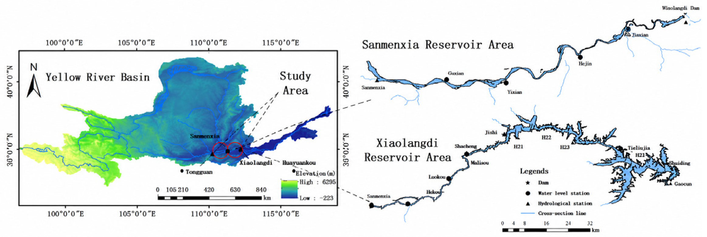
The study area is located in the segment below Tongguan in the middle reaches of the Yellow River, encompassing the Sanmenxia Reservoir and the Xiaolangdi Reservoir, as illustrated in Figure 1. These two reservoirs operate in succession, forming a cascade reservoir system that plays a vital role in flood control, sediment regulation, and water resource management. The region is characterized by a semi-arid climate, with an average annual precipitation ranging from 300 to 600 mm. Notably, over 10% of the annual rainfall occurs during the flood season (July to October), leading to severe soil erosion. The average annual sediment discharge reaches 1.6 billion tons, accounting for approximately 90% of the total sediment load in the entire Yellow River Basin.

The Sanmenxia Reservoir, commissioned in 1960, was primarily designed for flood control, irrigation, hydropower generation, and sediment retention. Since the implementation of the “318 Water Level Control Operation” prototype tests, the water–sediment conditions have undergone dramatic shifts. The inflow sediment load has exhibited a downward trend, and the effective reservoir capacity has been progressively recovering [21]. However, issues regarding capacity evolution and sediment regulation remain prominent, imposing higher requirements on the reservoir’s long-term operational functions.

The Xiaolangdi Reservoir began operations in 1999 with a total capacity of 12.65 billion m³. However, its long-term effective capacity is only 5.1 billion m³ [22]. As of October 2022, the cumulative sediment siltation has reached 3.467 billion m³. Although the ‘Water and Sediment Regulation’ (WSR) operational mode has effectively enhanced sediment discharge efficiency, it has not fully reversed the long-term trend of sediment accumulation. Consequently, the reservoir continues to face significant challenges regarding cumulative capacity maintenance and sustainable sediment management.

This study utilizes hydrological monitoring data from 2002 to 2022, covering the period since the implementation of the “Water and Sediment Regulation” scheme in the Yellow River Basin. The dataset includes daily average discharge and sediment concentration data from the Tongguan, Sanmenxia, and Xiaolangdi hydrological stations, as well as forebay water level data from the Shijiatan (II) stage station and the Tongshuling water–sediment factor station. All the aforementioned data were obtained from the Hydrological Yearbook of the Yellow River Basin. Reservoir capacity data were derived through calculations based on the established stage capacity curves. The statistical characteristics of the outflow water and sediment data for the two reservoirs during the study period are summarized in

Table 1. Statistical characteristics of outflow water and sediment data.

Region	Data Category	Average Value	Standard Deviation	Coefficient of Variation *	Skewness *	Maximum Value	Minimum Value
Sanmenxia Reservoir	Outflow Discharge (m3/s)	836.13	700.82	0.838	2.77	8000.00	2.23
	Outflow Sediment Concentration (kg/m3)	5.66	24.33	4.296	9.29	457.14	0.00
Xiaolangdi Reservoir	Outflow Discharge (m3/s)	889.90	752.13	0.845	2.37	5160.00	83.30
	Outflow Sediment Concentration (kg/m3)	1.84	12.00	6.523	11.64	289.30	0.00

* Indicates that the parameter is dimensionless.

.

The statistical characteristics presented in Table 1 reveal the inherent complexity of the outflow water and sediment data. In particular, the sediment concentration exhibits exceptionally high skewness (up to 11.64) and high coefficients of variation (up to 6.523), indicating highly skewed distributions characterized by extreme fluctuations. Such statistical properties pose significant challenges for traditional linear models, thereby justifying the necessity of employing advanced non-linear deep learning architectures to capture the complex dynamics of the system.

3. Materials and Methods

3.1. Deep Learning Methods

3.1.1. CNN

When processing time-series data, Convolutional Neural Networks (CNNs) can automatically extract local features through convolution operations, which helps the model identify short-term dependency patterns within the sequence.

Suppose the input is a one-dimensional vector x = [x₁, x₂, …, x_n]. A convolutional layer contains c filters, where the c-th filter is denoted as w^(c) = [w₁^(c), w₂^(c), …, w_k^(c)]. In this study, a single 1D convolutional layer is implemented. For a convolutional layer with a kernel size of k, the convolution operation is defined as follows:

$$y_i^{\left(\mathrm{c}\right)}={\displaystyle \sum _{j=1}^k{x}_{i+j-1}\cdot w_j^{\left(\mathrm{c}\right)}+b^{\left(\mathrm{c}\right)}},i=1,2,\dots ,\mathrm{n}-\mathrm{k}+1$$

(1)

where y_i^(c) is the output convolutional feature; x_i+j−1 represents the element in the input data corresponding to the kernel weight w_j^(c); and b^(c) denotes the bias term.

The output of the convolution operation is transformed via a non-linear activation function σ. In this study, the Rectified Linear Unit (ReLU) function is employed, which is defined as follows:

$$\sigma \left(y_i^{\left(\mathrm{c}\right)}\right)=\max \left(0,y_i^{\left(\mathrm{c}\right)}\right)$$

(2)

When y_i^(c) ≥ 0, the function outputs y_i^(c), thereby retaining the input value directly; when y_i^(c) < 0, the function outputs 0.

The pooling layer is used for downsampling to reduce the length of the feature maps while retaining the most prominent features. Assuming a pooling window size of p, the calculation of the max-pooling layer at each position z_i^(c) is defined as follows:

$$z_i^{\left(\mathrm{c}\right)}=\max \left(y_i^{\left(\mathrm{c}\right)},y_{i+1}^{\left(\mathrm{c}\right)},\dots ,y_{i+p-1}^{\left(\mathrm{c}\right)}\right)$$

(3)

where y_i^(c), y_i+1^(c), …, y_i+p−1^(c) are the convolution output values within the pooling window; the maximum value among them is selected as the output after the pooling operation.

The output of the pooling layer is a multi-dimensional array, which is converted into a one-dimensional vector through a flattening layer. Assuming the output of the pooling layer is a vector z = [z₁, z₂, …, z_m], its form remains unchanged after the flattening operation. The flattened vector then enters the fully connected (FC) layer. Let the weights of the fully connected layer be w = [w₁, w₂, …, w_m] and the bias term be b. The output of the fully connected layer serves as the final output of the model:

$$\stackrel{\wedge }{y}={\displaystyle \sum _{i=1}^m{z}_i\cdot w_i+b}$$

(4)

3.1.2. LSTM

Long Short-Term Memory (LSTM) is a sophisticated recurrent neural network architecture developed by Hochreiter and Schmidhuber to overcome the limitations of traditional RNNs. In the following formulations, the symbol $\otimes$ denotes the Hadamard product, which represents the element-wise multiplication of two vectors or matrices of the same dimension.

In this study, a model is constructed with two LSTM layers, where each LSTM unit comprises a forget gate, an input gate, and an output gate. The forget gate determines whether the information is retenained or discarded from the previous cell state c_t−1 passed from the preceding time step. Its calculation formula is as follows:

$$f_t=\sigma \left(W_f\cdot \left[h_{t-1},x_t\right]+b_f\right)$$

(5)

where f_t is the output of the forget gate; x_t and h_t−1 represent the input data at the current time step and the hidden state from the previous time step, respectively; W_f and b_f denote the weight matrix and bias term of the forget gate; and σ is the sigmoid activation function.

The input gate controls how the information from the current time step is updated into the cell state. This process consists of two steps. First, an input gate (i_t) determines which new information will be incorporated into the cell state:

$$i_t=\sigma \left(W_i\cdot \left[h_{t-1},x_t\right]+b_i\right)$$

(6)

Next, a candidate cell state is generated to create the new information content:

$$\widetilde{C_t}=\tanh \left(W_C\cdot \left[h_{t-1,}{x}_t\right]+b_C\right)$$

(7)

The final effect of the input gate is to combine these two components to store the new information into the cell state:

$$C_t=f_t\otimes C_{t-1}+i_t\otimes \widetilde{C_t}$$

(8)

The output gate controls the hidden state (h_t) at the current time step. It extracts the necessary information from the cell state and determines which information should be passed to the next layer or the subsequent time step. The formula is as follows:

$$o_t=\sigma \left(W_o\cdot \left[h_{t-1},x_t\right]+b_o\right)$$

(9)

$$h_t=o_t\otimes \tanh \left(C_t\right)$$

(10)

where o_t is the control variable of the output gate.

3.1.3. CNN-LSTM

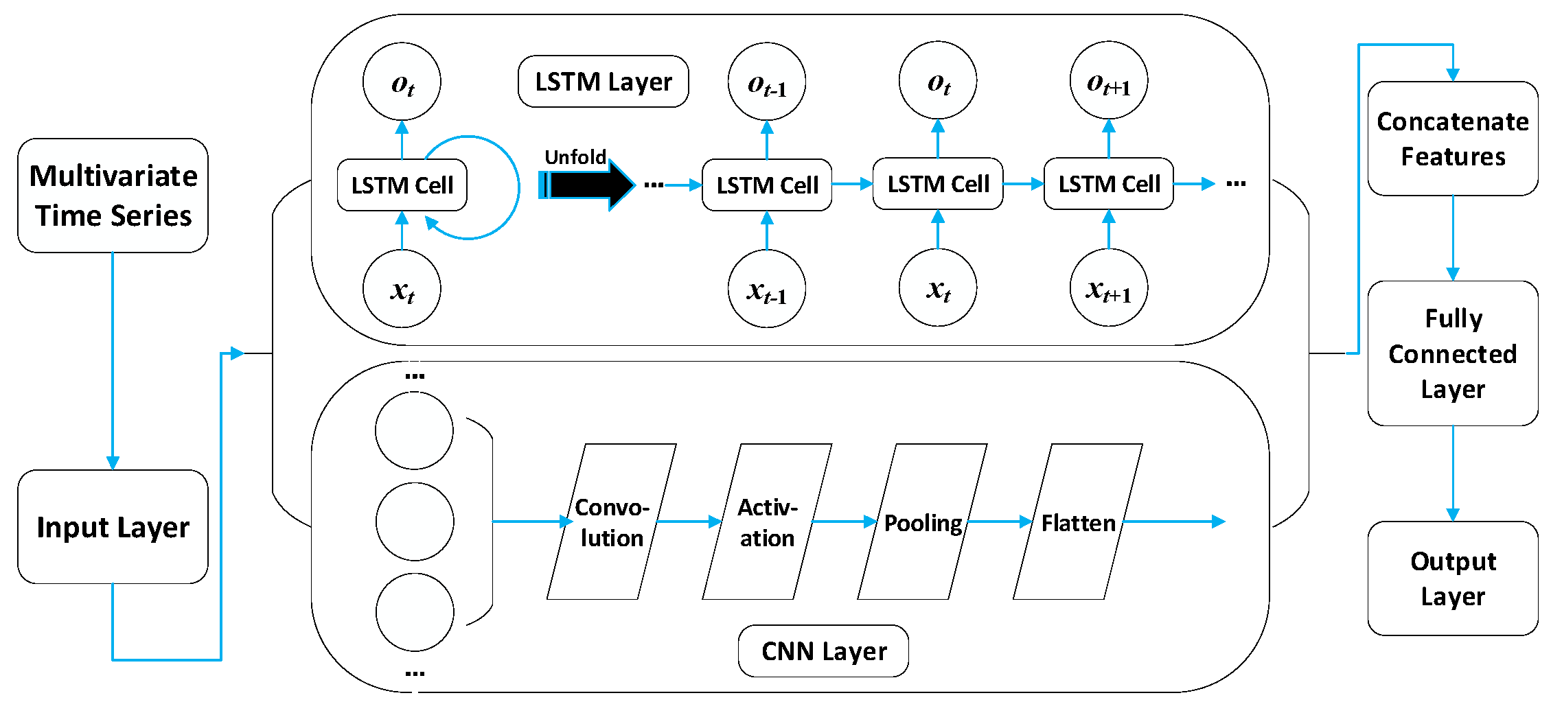
There are various coupling configurations for Convolutional Neural Network-Long Short-Term Memory (CNN-LSTM) hybrid architectures. This study adopts a parallel structure, as illustrated in Figure 2. The primary advantage of this configuration lies in its capability to simultaneously capture both local and global features within the sequence. Specifically, the CNN effectively extracts local features from the input sequence through its convolutional layers, while the LSTM learns long-term dependencies to capture global information.

This combination enables the model to focus on both fine-grained details and overall patterns, thereby enhancing its ability to recognize complex relationships. In summary, the CNN extracts low-level features at the bottom layer, while the LSTM extracts abstract features at a higher level. The integration of these two components facilitates comprehensive feature extraction across different hierarchical levels, leading to a more accurate understanding of the input sequence.

3.1.4. TCN

The Temporal Convolutional Network (TCN) is a time-series modeling approach based on convolutional neural networks, consisting of an input layer, causal dilated convolutional layers, and an output layer. In this study, a single TCN layer is implemented for feature extraction. Compared to traditional recurrent neural networks, TCN offers superior parallel computing capabilities and exhibits greater stability during long-sequence modeling.

The core computational unit of the TCN is the causal dilated convolutional layer. The causal convolution structure ensures that the output at each time step depends only on the current and previous input data, thereby preventing the issue of future information leakage. Meanwhile, the dilated convolution mechanism significantly expands the receptive field by introducing a dilation rate, d, while maintaining a constant kernel size. Its calculation formula can be expressed as:

$$y_t=\sigma ({\displaystyle \sum _{i=0}^{k-1}{w}_i}\cdot x_{t-d\cdot i}+b)$$

(11)

where σ is the activation function, and the ReLU function is employed in this study; y_t is the output at time step t; x_t−d·i represents the input at time step t−d·i; w denotes the convolutional kernel of size k; d is the dilation rate; and b is the bias term. As d increases, the receptive field of the convolutional layer expands exponentially, enabling the model to capture long-range dependencies without significantly increasing computational complexity.

3.2. Optimization Algorithm

In this study, the Genetic Algorithm (GA) is employed to optimize the hyperparameters of each prediction model. GA simulates the evolutionary process of “survival of the fittest” in nature. The optimization is an iterative process based on a population, which gradually evolves toward the optimal or near-optimal solution through genetic operations such as selection, crossover, and mutation.

To simultaneously handle discrete and continuous hyperparameters and adapt to the different constraints of flow and sediment concentration prediction, the GA has been improved. The primary modifications include:

(1)

Individual encoding and population initialization: A hybrid chromosome encoding method is adopted to represent the hyperparameters of the prediction model. For an individual (i.e., a specific combination of hyperparameters), it can be expressed as a vector:

$$x=\left[p_1,p_2,\dots ,p_d\right]$$

(12)

where x represents an individual, d is the total number of hyperparameters, and p_i denotes the i-th hyperparameter. Real-number encoding is employed for continuous hyperparameters, while integer encoding is used for discrete parameters.

(2)

Fitness function design: A fitness function that integrates the Nash–Sutcliffe Efficiency (NSE) and physical constraints is established:

$$f(x)=NSE(x)-\lambda \cdot P(x)$$

(13)

$$P(x)={\displaystyle \sum _{i=1}^N\max }(0,-y_{pred,i})$$

(14)

where P(x) is the penalty term, which applies a weighted penalty to negative prediction values; λ is the penalty coefficient used to control the intensity of the penalty.

Note that the physical non-negative constraint is enforced exclusively during the post-processing phase, after inverse-transforming the model outputs back to their original hydrological scale.

To ensure search efficiency, the population size in this study is set to 10, and the maximum number of iterations is set to 20. This configuration is motivated by a preliminary sensitivity analysis, which indicated that the fitness function reaches a stable plateau within 20 iterations, suggesting that further iterations offer diminishing returns. Moreover, the search space for the hyperparameters was pre-constrained based on expert domain knowledge, effectively limiting the scope to a focused region where the global optimum is likely to reside. An elitist strategy is employed, where the top 50% of individuals are retained based on their fitness ranking. The remaining population generates new individuals through single-point crossover and mutation operations. The crossover rate is set to 80%, and the mutation rate is set to 20%, with values randomly reset within boundaries according to the parameter types. The algorithm uses the attainment of the maximum number of iterations as the termination criterion, achieving a robust balance between computational efficiency and optimization performance.

4. Prediction Model for the Reservoir Water–Sediment Process

4.1. Feature Variable Selection

In the predictive modeling of reservoir outflow and sediment processes, the scientific and reasonable selection of input feature variables is a critical step in enhancing model performance. For outflow (Q_in) prediction, the candidate variables primarily include inflow (Q_out), inflow sediment concentration (S_in), outflow sediment concentration (S_out), water level at the inflow station (H_in), water level in front of the dam (H_dam), and reservoir capacity (V). Since the Sanmenxia and Xiaolangdi reservoirs form a cascade system, the inflow of the upstream reservoir significantly affects the outflow of the downstream reservoir. Therefore, in the outflow prediction for the Xiaolangdi Reservoir, the upstream inflow (Q_{up in}) is incorporated into the variable set. For S_out prediction, the candidate variables mainly include Q_in, Q_out, S_in, H_in, H_dam, the water level difference between the inflow station and the dam (ΔH), and V.

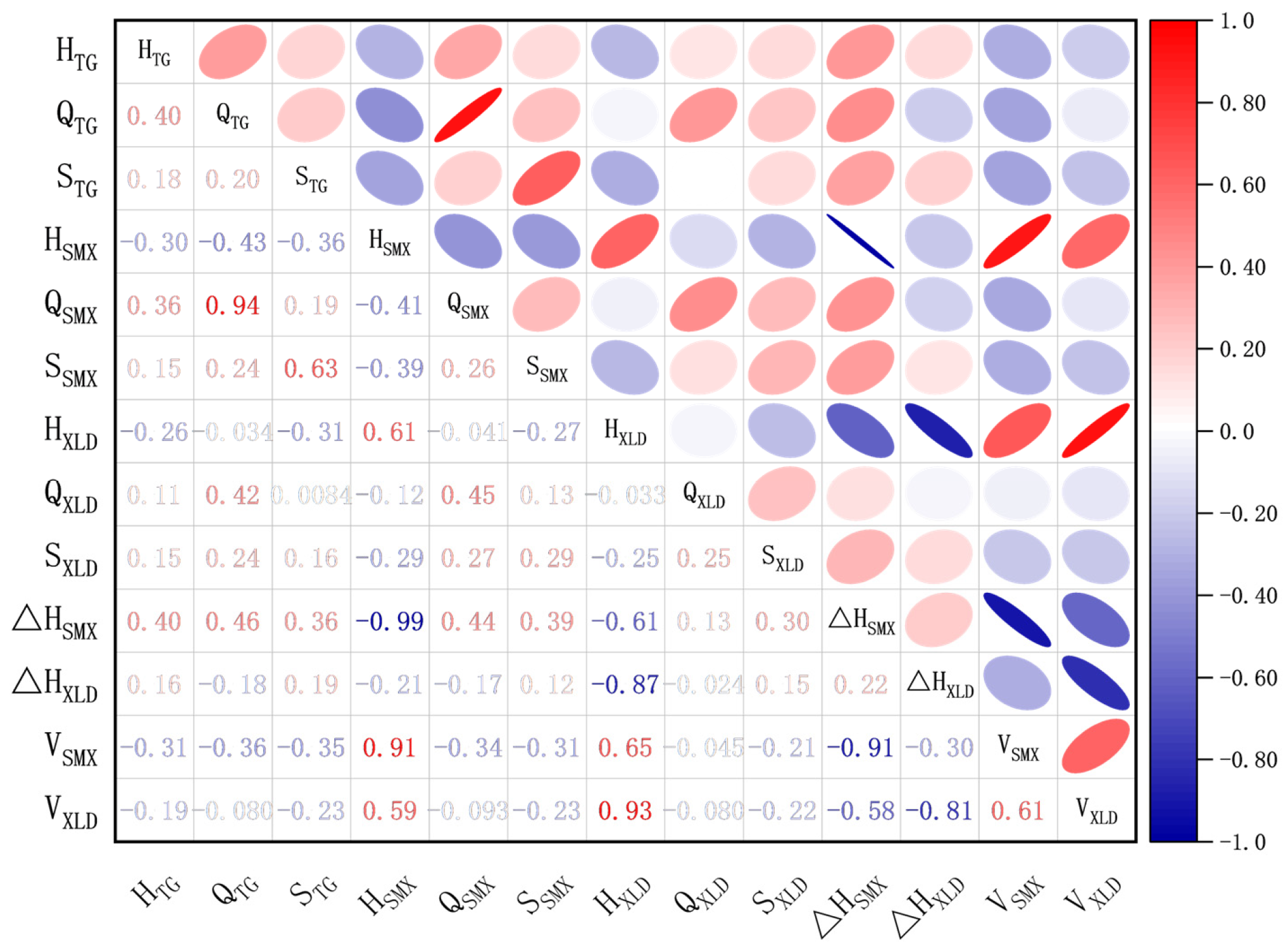
This study employs the Pearson correlation coefficient to evaluate the linear correlation between each candidate variable and the target variable, with a correlation heatmap (Figure 3) generated for visual analysis. The results indicate that for the Sanmenxia Reservoir, H_in, Q_in, H_dam, and V exhibit strong correlations with Q_out, while Q_in, Q_out, S_in, ΔH, H_dam, and V show strong correlations with S_out. For the Xiaolangdi Reservoir, Q_in and Q_{up in} are strongly correlated with Q_out, whereas Q_in, Q_out, S_in, H_dam, and V are strongly correlated with S_out. Consequently, these selected variables are utilized as feature variables for the model input.

4.2. Model Construction

Based on the open-source deep learning framework PyTorch (1.10.2) and CNN, LSTM, and TCN algorithms, the prediction models for the reservoir outflow and sediment processes of the Sanmenxia and Xiaolangdi reservoirs in the middle reaches of the Yellow River were established using Python (3.12). The specific procedure is as follows:

(1)

Data cleaning: Missing values and outliers in the original data were first detected and corrected. Missing values were filled using linear interpolation, while outliers were corrected based on empirical rules or upper/lower threshold limits to ensure data integrity and reliability.

(2)

Normalization and standardization: For flow prediction, the data x₁ underwent Min–Max normalization to linearly map the values to the range of [−1, 1], reducing the impact of different dimensions on model training. Given the significant presence of zero values and the skewed distribution in the sediment concentration series, Z-score standardization was applied to the data x₂ to transform it into a distribution with a mean of 0 and a standard deviation of 1. All processing was performed based on the training set.

(3)

Optimizer and loss function settings: Corresponding optimizers and loss functions were selected for different deep learning algorithms.

(4)

Feature selection and sample construction: The feature variables selected in Section 3.1 were combined with the target variables to construct the initial input dataset. To maintain the continuity and dynamic characteristics of the time series, a sliding window mechanism was used for sample generation. The window length was set to 7, using feature data from seven consecutive days as model input to predict the target variable for the 8th day (i.e., a 1-day lead time).

(5)

Model training and parameter optimization: The dataset was chronologically divided into a training set (1 January 2002–26 September 2018), a validation set (27 September 2018–13 November 2020), and a test set (14 November 2020–31 December 2022) at a ratio of 8:1:1. Four models were trained on the training set, the improved Genetic Algorithm (GA) was used for hyperparameter optimization on the validation set, and the optimal hyperparameters were used on the test set to evaluate prediction performance.

To assess model performance, four evaluation metrics were employed: Mean Absolute Error (MAE), Root Mean Square Error (RMSE), Nash–Sutcliffe Efficiency (NSE), and Kling–Gupta Efficiency (KGE). All prediction tasks in this study were conducted through five independent repeated experiments, with the average values used as the final measure of model performance.

5. Results and Analysis

5.1. Optimal Hyperparameters of the Model

The performance of deep learning models in hydrological series prediction highly depends on the appropriate configuration of their hyperparameters. To ensure that the deep learning models applied to the outflow and sediment prediction for the Sanmenxia and Xiaolangdi reservoirs achieve optimal performance on unseen data, a Genetic Algorithm (GA) was employed for hyperparameter optimization on the validation set. Through GA optimization, the optimal hyperparameters for the different models at each reservoir were determined.

Table 2. Optimal hyperparameter combinations for outflow and sediment prediction models in the Sanmenxia Reservoir.

Model	Variable	No. of Filters	Kernel Size	Stride	Learning Rate	Epochs
CNN	Q	128	2	3	0.0009	85
	S	64	2	2	0.0031	124
Model	Variable	Hidden Units	Dropout Rate	—	Learning Rate	Epochs
LSTM	Q	89	0.14	—	0.0006	122
	S	90	0.16	—	0.0084	176
Model	Variable	No. of Filters	Kernel Size	Hidden Units	Learning Rate	Epochs
CNN-LSTM	Q	128	3	92	0.001	138
	S	128	3	96	0.0011	161
Model	Variable	No. of Filters	Kernel Size	Dilation Rates	Learning Rate	Epochs
TCN	Q	128	3	[1, 2, 4, 8]	0.0008	44
	S	64	4	[1, 2, 4, 8]	0.0016	181

and

Table 3. Optimal hyperparameter combinations for outflow and sediment prediction models in the Xiaolangdi Reservoir.

Model	Variable	No. of Filters	Kernel Size	Stride	Learning Rate	Epochs
CNN	Q	128	2	3	0.0009	85
	S	128	2	2	0.0031	103
Model	Variable	Hidden Units	Dropout Rate	—	Learning Rate	Epochs
LSTM	Q	86	0.18	—	0.0006	143
	S	84	0.11	—	0.0084	176
Model	Variable	No. of Filters	Kernel Size	Hidden Units	Learning Rate	Epochs
CNN-LSTM	Q	128	2	88	0.001	149
	S	128	2	88	0.0036	193
Model	Variable	No. of Filters	Kernel Size	Dilation Rates	Learning Rate	Epochs
TCN	Q	128	3	[1, 2, 4, 8]	0.0007	35
	S	128	4	[1, 2, 4, 8]	0.0025	172

detail the best combinations for each model in the Sanmenxia and Xiaolangdi reservoirs, respectively.

Model parameter configurations exhibit significant task-specific sensitivity. Overall, convolutional models generally adopt a higher number of filters (64 or 128), with kernel sizes concentrated between 2 and 3. This indicates that in water–sediment time-series modeling, local feature extraction is more sensitive to sudden peak values; small-scale, multi-channel convolutions significantly enhance the models’ ability to learn nonlinear water–sediment sequences. The dilation rates for the TCN are all set to [1, 2, 4, 8] to ensure that the multi-scale receptive field covers long-term dependency features. In recurrent structures, the number of hidden units is concentrated between 86 and 96, balancing feature extraction capability with generalization performance. Dropout rates range from 0.11 to 0.18, suggesting that moderate regularization improves model stability.

The learning rates are generally on the order of 0.001, with those for outflow prediction tasks being consistently lower than those for sediment concentration prediction. This suggests that outflow prediction is more sensitive to the learning rate. Since flow sequences are relatively stable, a lower learning rate helps the model converge precisely under small gradients. Conversely, sediment concentration prediction is highly sensitive to both the learning rate and the number of epochs. Due to the violent fluctuations in sediment sequences, a higher learning rate combined with more epochs is required to learn extreme peaks. The number of epochs ranges from 35 to 193, while the TCN requires fewer iterations in some tasks, indicating a faster convergence speed facilitated by its dilated convolution mechanism. In summary, the CNN-LSTM achieves a balanced configuration across kernel size, hidden units, learning rate, and epochs, fully integrating local features and long-term dependencies, which establishes the foundation for its overall optimal performance in subsequent prediction tasks.

5.2. Overall Model Evaluation

This section aims to provide a comprehensive evaluation of the performance of four deep learning models in predicting the reservoir outflow and sediment processes in the Sanmenxia and Xiaolangdi reservoirs. According to the evaluation metrics for the Sanmenxia Reservoir presented in

Table 4. Comparison of evaluation metrics for outflow and sediment prediction models in the Sanmenxia Reservoir.

Model	Q				S
	RMSE (m3/s)	MAE (m3/s)	NSE	KGE	RMSE (kg/m3)	MAE (kg/m3)	NSE	KGE
CNN	286.052	180.593	0.903	0.920	7.777	1.542	0.759	0.764
LSTM	268.289	164.693	0.915	0.945	7.208	1.007	0.793	0.797
CNN-LSTM	249.270	156.451	0.927	0.962	6.705	0.879	0.821	0.836
TCN	253.483	157.250	0.924	0.959	6.747	0.898	0.819	0.834

, the CNN-LSTM hybrid model exhibits the most prominent performance. In the outflow prediction, it achieves the lowest RMSE of 249.270 m³/s and MAE of 156.451 m³/s, while yielding the highest NSE of 0.927 and KGE of 0.962. Similarly, in the sediment concentration prediction, the CNN-LSTM model delivers the optimal results, with an RMSE of 6.705 kg/m³, MAE of 0.879 kg/m³, NSE of 0.821, and KGE of 0.836, fully demonstrating its high-precision predictive capability for this reservoir. The TCN model shows metrics very close to those of the CNN-LSTM. While the LSTM model also performs well, the standalone CNN model exhibits the poorest performance, with its four evaluation metrics further confirming its limitations in handling hydrological series with strong temporal dependencies.

Regarding the evaluation results for the Xiaolangdi Reservoir (

Table 5. Comparison of evaluation metrics for outflow and sediment prediction models in the Xiaolangdi Reservoir.

Model	Q				S
	RMSE (m3/s)	MAE (m3/s)	NSE	KGE	RMSE (kg/m3)	MAE (kg/m3)	NSE	KGE
CNN	236.059	142.103	0.932	0.933	6.073	0.996	0.802	0.786
LSTM	215.276	125.237	0.943	0.945	5.773	0.929	0.822	0.849
CNN-LSTM	203.834	122.343	0.949	0.963	5.421	0.848	0.843	0.864
TCN	213.483	123.250	0.944	0.963	5.549	0.865	0.835	0.858

), the CNN-LSTM model maintains its leading position. For outflow prediction, it yields an RMSE of 203.834 m³/s and an MAE of 122.343 m³/s, with NSE and KGE values of 0.949 and 0.963, respectively. For sediment concentration prediction, its RMSE of 5.421 kg/m³ and MAE of 0.848 kg/m³, along with NSE and KGE of 0.843 and 0.864, outperform those of all other models. Notably, the TCN model achieves a KGE of 0.963 for outflow prediction, equaling that of the CNN-LSTM, which indicates that the TCN reaches the same balance as the optimal model in capturing the mean, variability, and correlation of the Xiaolangdi Reservoir’s flow process. The LSTM model continues to perform well, whereas the CNN remains the weakest performer.

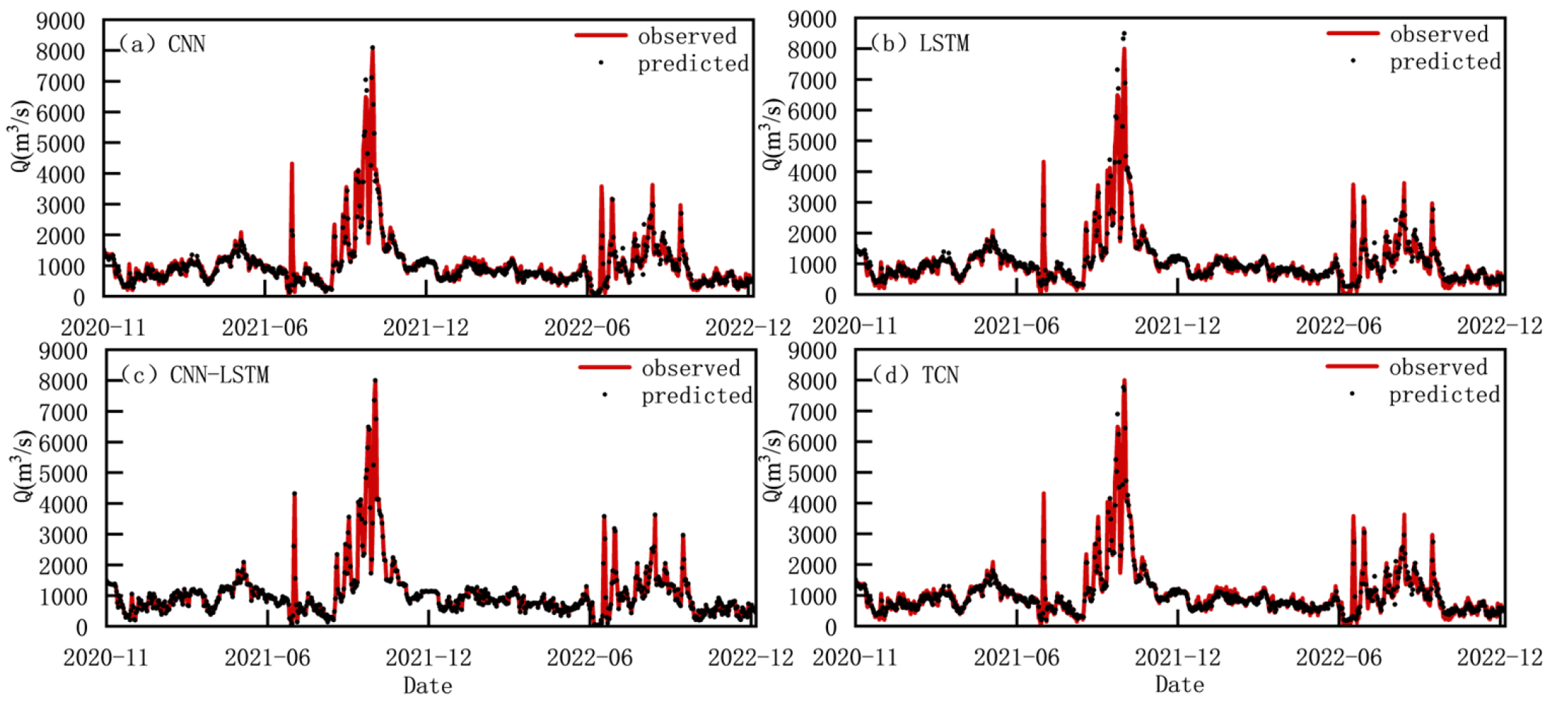
Comparing the evaluation results of both reservoirs, the CNN-LSTM model demonstrates superior and stable predictive capability across both locations. The TCN model also exhibits robust performance. Interestingly, all models yield lower RMSE and MAE values and higher NSE and KGE values for the Xiaolangdi Reservoir compared to the Sanmenxia Reservoir. This suggests that the water–sediment process in the Xiaolangdi Reservoir is relatively more regular, with less data noise, making it easier for the models to learn. In contrast, the evolution of water and sediment in the Sanmenxia Reservoir is more complex, driven by rapid backwater fluctuations and intense deposition–erosion cycles. These nonlinear interactions between reservoir dispatching and channel morphology impose higher requirements on model generalization (Figure 4).

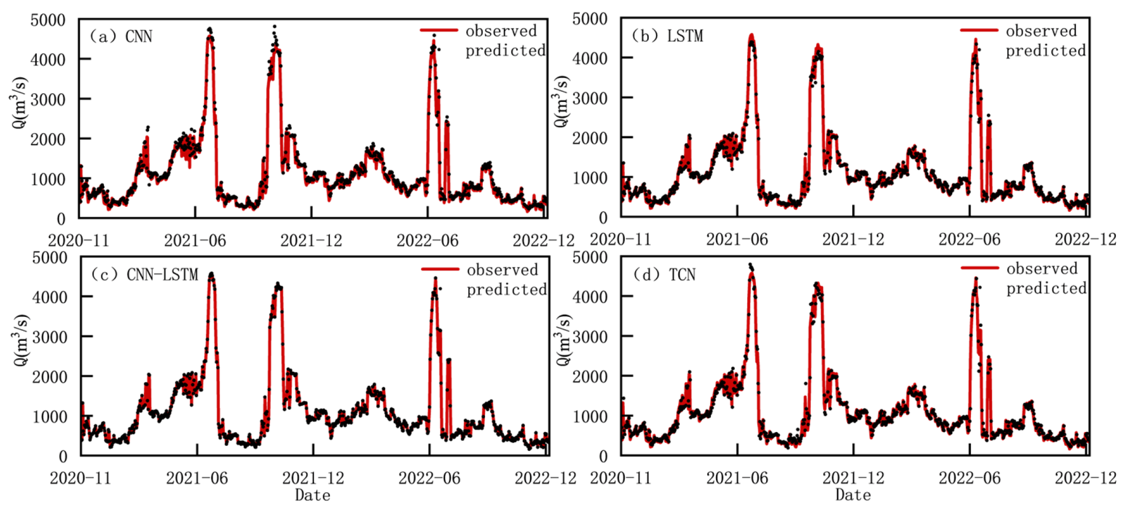
Figure 4. Comparison of predicted results from different models for outflow in the Sanmenxia Reservoir on the test set.

Figure 4. Comparison of predicted results from different models for outflow in the Sanmenxia Reservoir on the test set.

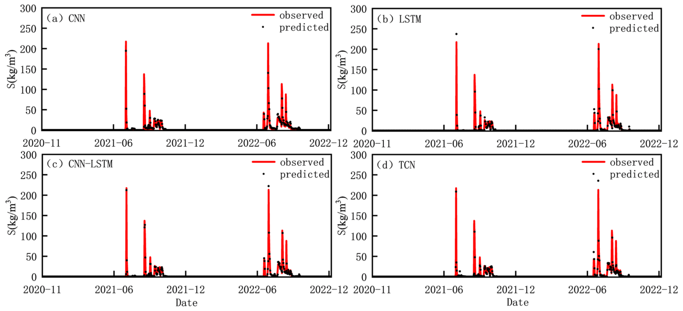
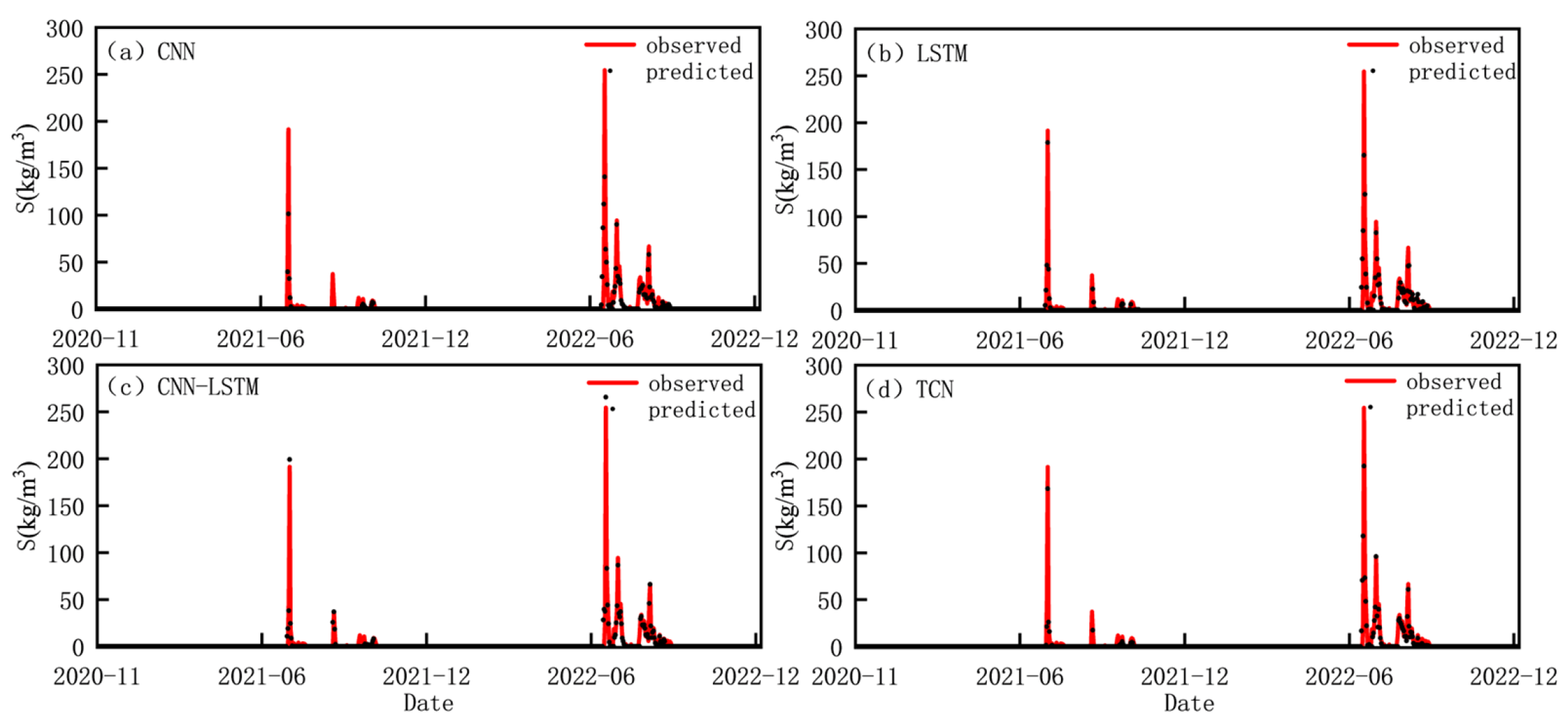
Figure 5, Figure 6, Figure 7 and Figure 8 illustrate the comparison between the predicted values (black dots) and the actual observed values (red curves) for reservoir outflow and sediment concentration across all models on the test set for the Sanmenxia and Xiaolangdi reservoirs. From the visualization results, it is clearly observed that the CNN-LSTM model exhibits higher prediction accuracy compared to the other models for both outflow and sediment concentration at both reservoirs. Its predicted values are highly consistent with the observed data, showing smaller lags and lower biases when capturing key hydrological events such as rapid changes in flow and sediment, as well as flood and sediment peaks. The TCN and LSTM models also show favorable predictive performance, effectively capturing hydrological trends; however, they exhibit slight discrepancies in the precision of predicting peaks or troughs compared to the CNN-LSTM model. In contrast, the standalone CNN model performs the poorest. Its prediction curves deviate significantly from the actual values for both flow and sediment at both reservoirs, demonstrating its limitations in predicting data with strong temporal dependencies. Overall, the capability to capture sediment peaks is lower than that for flow peaks across all models, likely due to the higher inherent volatility and unpredictability of sediment data.

Further error analysis indicates that for the Sanmenxia Reservoir under high-flow conditions (>2000$ m³/s), the Mean Relative Errors (MREs) for CNN, LSTM, CNN-LSTM, and TCN are 17.45%, 16.56%, 15.62%, and 16.01%, respectively. Under high-sediment conditions (>10$ kg/m³), the MREs are 30.23%, 23.55%, 19.51%, and 42.84%, respectively, with TCN exhibiting the largest error. For the Xiaolangdi Reservoir, under high-flow conditions, the MREs of the four models are 10.36%, 10.34%, 9.84%, and 10.09%, respectively; under high-sediment conditions, they are 41.52%, 53.76%, 28.86%, and 33.46%, respectively, with LSTM showing the maximum error. These results demonstrate that the CNN-LSTM maintains superior stability and accuracy across different conditions, which is highly consistent with the visualization findings, further highlighting its comprehensive advantages in predicting reservoir outflow and sediment processes.

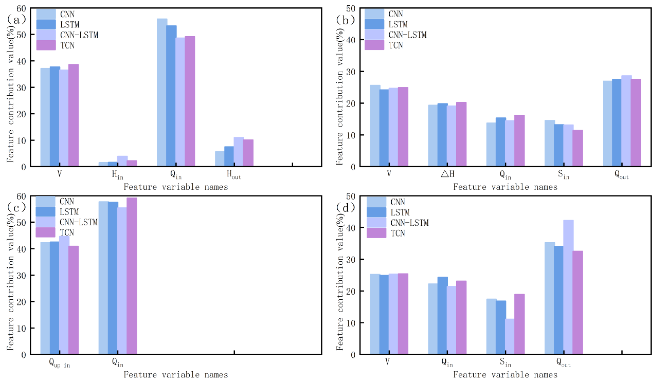
To quantify the decision-making mechanisms of each deep learning model in water–sediment prediction for the Sanmenxia and Xiaolangdi Reservoirs, this study introduces the SHAP (SHapley Additive Explanations) attribution method to reveal the models’ decision-making mechanisms. As shown in Figure 8, in terms of outflow prediction, the Sanmenxia Reservoir is dominated by two variables—inflow and reservoir capacity—with feature weight values exceeding 45% and 35%, respectively. In contrast, the Xiaolangdi Reservoir exhibits pronounced cascade coupling characteristics, driven by the superimposed inflow from both the upstream station and the reservoir itself, with feature weight values exceeding 40% and 55%, respectively.

In terms of sediment concentration prediction, the feature contributions shift from being flow-dominated to being driven by the coordination of multi-source water and sediment variables, with almost all feature weight values exceeding 15%. The models effectively identify the dynamic reshaping effects of water level differences and reservoir capacity on sediment transport.

These SHAP results provide direct evidence that the model effectively integrates the dynamic interactions between water–sediment evolution and reservoir storage–discharge states, thus overcoming the limitations of single time-series models mentioned in the introduction.

6. Discussion

This study systematically compares the prediction of reservoir outflow and sediment processes for the Sanmenxia and Xiaolangdi reservoirs. The results indicate that the CNN-LSTM model achieves the optimal performance across both reservoirs, outperforming other models in all evaluation metrics and demonstrating prominent capability in capturing flow and sediment peaks. This is consistent with the synergistic advantage noted by Ghimire et al. [23], who stated that “CNNs are utilized for local feature extraction while LSTMs capture temporal information.” It also aligns with findings from related research [24], which suggest that intelligent optimization algorithms combined with hybrid models possess stronger generalization capabilities for complex hydrological series.

The predictive difficulty differs significantly between the two reservoirs. All models performed better on the Xiaolangdi Reservoir, likely due to its lower data noise and clearer operational patterns. In contrast, the Sanmenxia Reservoir, as a typical siltation-type reservoir, operates under the “storing clear water and discharging muddy water” mode. This process is accompanied by intense riverbed erosion and deposition evolution, as well as sediment resuspension, leading to greater fluctuations in the water–sediment series. These factors significantly increase the difficulty for the models in capturing underlying physical features, a finding consistent with Wang et al. [25]. Furthermore, the prediction errors for sediment peaks across all four models were generally larger than those for flow peaks, indicating that the high volatility and abruptness of sediment concentration series remain major challenges for deep learning models [26].

The interpretability analysis via SHAP reveals that the model’s predictive performance is not merely a mathematical optimization but a reflection of physical hydrological processes. Specifically, the significant feature importance weights assigned to sediment inflow and water level during the flood season indicate the model’s sensitivity to the “storing clear water and discharging muddy water” operational mode of the Sanmenxia Reservoir. As shown in Figure 8, the reallocation of feature importance weights during periods of intense riverbed erosion and sediment resuspension provides direct evidence that the model effectively captures the physical transition from deposition to resuspension. This demonstrates that the machine learning decision-making mechanism is physically grounded in the complex, non-linear sediment evolution processes inherent to the reservoir system.

This connection between SHAP-derived feature importance and real-world sediment dynamics bridges the gap between data-driven outcomes and hydrological theory. The higher predictive errors observed in the Sanmenxia Reservoir, compared to the Xiaolangdi Reservoir, can now be physically interpreted: the model encounters greater challenges when the SHAP weights exhibit high volatility, which corresponds precisely to the non-linear sediment resuspension and riverbed erosion phases. This suggests that the model’s performance is limited by the inherent physical complexity of these turbulent periods rather than simple statistical noise. Consequently, this study demonstrates that the model’s “intelligence” is derived from its ability to adapt to these physically turbulent phases by dynamically adjusting its feature reliance, rather than just overfitting to historical trends.

While deep learning demonstrates immense potential in water–sediment prediction, this study highlights the necessity of bridging data-driven models with physical mechanisms. Future research could further incorporate hydrological mechanism constraints (physics-informed) to explicitly embed these “storing clear water and discharging muddy water” operational rules into the model, thereby enhancing physical consistency. Furthermore, exploring the transfer learning capabilities of these models in other river basins could verify their universality across different sediment transport regimes. Finally, quantifying predictive uncertainty remains a critical research frontier, which would provide more comprehensive risk assessment information for reservoir operation and management under evolving climatic and human-induced conditions.

7. Conclusions

Based on water and sediment data, along with derived variables such as reservoir capacity, from the Sanmenxia and Xiaolangdi reservoirs in the middle reaches of the Yellow River, this study successfully developed prediction models for reservoir outflow and sediment processes by combining a Genetic Algorithm (GA) with four deep learning methods: CNN, LSTM, CNN-LSTM, and TCN. The results indicate that, within the parameter framework established in this study, the deep learning models can effectively capture the nonlinear and temporal characteristics of the water–sediment processes in both reservoirs.

Specifically, the CNN-LSTM hybrid model achieved the best overall performance. On the test set, its NSE values for outflow and sediment concentration prediction at the Sanmenxia Reservoir reached 0.927 and 0.821, respectively, while those for the Xiaolangdi Reservoir reached 0.949 and 0.843. These results fully demonstrate the effectiveness of integrating the local feature extraction advantages of CNNs with the long-sequence modeling capabilities of LSTMs. By explicitly incorporating reservoir capacity and key hydrological constraints, this study advances the field of intelligent reservoir operation by shifting from standard data-driven benchmarks toward physically aware decision-making. This approach addresses the research gap regarding the interpretability of traditional models, proving that machine learning can maintain physical consistency in complex operations, such as the “storing clear water and discharging muddy water” mode. The TCN model also demonstrated strong competitiveness.

Furthermore, this study confirms the inherent differences in water–sediment prediction between the two reservoirs, which exhibit distinct characteristics in terms of predictive difficulty and key influencing factors. The selection of feature variables was found to have a significant impact on the predictive performance of the models.

References

1. Zhao, Y.; Qu, B.; Jiang, E.H.; Li, E.F.; Liu, Y. Joint optimal regulation of Sanmenxia-Xiaolangdi reservoirs in flood season considering multi-source inflow and sediment. Yellow River 2024, 46, 44–48. (In Chinese) [Google Scholar]
2. Zhang, W.; Huang, H.; Su, C.; Wang, P.; Kong, Y.; Cui, Y. Water–sediment multi-objective synergetic scheduling of reservoirs considering reservoir–river coupling: A case study of the Middle and Lower Yellow River. Environ. Model. Softw. 2026, 202, 106987. [Google Scholar] [CrossRef]
3. Zhang, X.; Qiao, W.; Lu, Y.; Huang, J.; Xiao, Y. Quantitative analysis of the influence of the Xiaolangdi reservoir on water and sediment in the middle and lower reaches of the Yellow River. Int. J. Environ. Res. Public Health 2023, 20, 4351. [Google Scholar] [CrossRef] [PubMed]
4. Xia, J.; Zhang, X.; Zhou, M.; Cheng, Y.; Zhou, Z.; Wang, Z.; Wan, Z.; Falconer, R.A. Modeling study on enhancing overall sediment transport efficiency in a reservoir-river coupled system of the Middle and Lower Yellow River. Water Resour. Res. 2026, 62, e2025WR041342. [Google Scholar] [CrossRef]
5. Sungmin, O.; Dutra, E.; Orth, R. Robustness of process-based versus data-driven modeling in changing climatic conditions. J. Hydrometeorol. 2020, 21, 1929–1944. [Google Scholar] [CrossRef]
6. Herath, H.M.V.V.; Chadalawada, J.; Babovic, V. Hydrologically informed machine learning for rainfall–runoff modelling: Towards distributed modelling. Hydrol. Earth Syst. Sci. 2021, 25, 4373–4401. [Google Scholar] [CrossRef]
7. Zhang, X.Z.; Yang, L.H.; Song, X.F. Characteristics of water and sediment variations in the upper reaches of the Yellow River in recent 60 years and their influencing factors. J. Lake Sci. 2024, 36, 602–621. (In Chinese) [Google Scholar] [CrossRef]
8. Moges, E.; Demissie, Y.; Larsen, L.; Yassin, F. Sources of hydrological model uncertainties and advances in their analysis. Water 2021, 13, 28. [Google Scholar]
9. Sharafati, A.; Asadollah, S.B.H.S.; Motta, D.; Yaseen, Z.M. Application of newly developed ensemble machine learning models for daily suspended sediment load prediction and related uncertainty analysis. Hydrol. Sci. J. 2020, 65, 2022–2042. [Google Scholar] [CrossRef]
10. Ghobadi, F.; Kang, D. Application of machine learning in water resources management: A systematic literature review. Water 2023, 15, 620. [Google Scholar] [CrossRef]
11. Drogkoula, M.; Kokkinos, K.; Samaras, N. A comprehensive survey of machine learning methodologies with emphasis in water resources management. Appl. Sci. 2023, 13, 12147. [Google Scholar] [CrossRef]
12. Almubaidin, M.A.A.; Latif, S.D.; Balan, K.; Ahmed, A.N.; El-Shafie, A. Enhancing sediment transport predictions through machine learning-based multi-scenario regression models. Results Eng. 2023, 20, 101585. [Google Scholar] [CrossRef]
13. Fan, J.S.; Liu, X.F.; Li, W.D. Daily suspended sediment concentration forecast in the upper reach of Yellow River using a comprehensive integrated deep learning model. J. Hydrol. 2023, 623, 129732. [Google Scholar] [CrossRef]
14. Zhang, S.Q.; Zuo, Q.T.; Zang, C.; Zhang, L.K.; Ba, Y.J. Runoff simulation and future multi-scenario prediction in the Qinhe River Basin based on CNN-LSTM-Attention model. J. Water Resour. Water Eng. 2024, 35, 73–81. (In Chinese) [Google Scholar]
15. Ma, D.; Yang, C.; Tian, Q.; Guo, L. Analysis and prediction of monthly runoff evolution characteristics in Linqi reservoir (China). Front. Environ. Sci. 2026, 14, 1785661. [Google Scholar] [CrossRef]
16. Fan, J.; Li, R.; Zhao, M.; Pan, X. A BiLSTM-Based Hybrid Ensemble Approach for Forecasting Suspended Sediment Concentrations: Application to the Upper Yellow River. Land 2025, 14, 1199. [Google Scholar] [CrossRef]
17. Ding, Y.D.; Jiang, M.L.; Xu, L.G.; Fan, H.X.; Lv, H.S. Reservoir flood forecasting using long short-term memory model based on whale optimization algorithm. J. Lake Sci. 2024, 36, 320–332. (In Chinese) [Google Scholar]
18. Kilinc, H.C.; Apak, S.; Ergin, M.E.; Ozkan, F.; Katipoğlu, O.M.; Yurtsever, A. Enhancing hydrological time series forecasting with a hybrid Bayesian-ConvLSTM model optimized by particle swarm optimization. Acta Geophys. 2025, 74, 3549–3566. [Google Scholar] [CrossRef]
19. Aoulmi, Y.; Marouf, N.; Rasouli, K.; Panahi, M. Runoff predictions in a semiarid watershed by convolutional neural networks improved with metaheuristic algorithms and forced with reanalysis and climate data. J. Hydrol. Eng. 2023, 28, 04023018. [Google Scholar] [CrossRef]
20. Jhong, Y.-D.; Chen, C.-S.; Jhong, B.-C.; Tsai, C.-H.; Yang, S.-Y. Optimization of LSTM parameters for flash flood forecasting using genetic algorithm. Water Resour. Manag. 2024, 38, 1141–1164. [Google Scholar] [CrossRef]
21. Yang, G.B.; Wu, B.S.; Zhang, R.Y.; Shang, H.X. Influence of “318” regulation of Sanmenxia Reservoir on the elevation change of Tongguan. J. Sediment Res. 2020, 45, 38–45. (In Chinese) [Google Scholar]
22. Zhang, J.L.; Lu, J.; Wei, S.T.; Luo, Q.S.; Wan, Z.W. Reasons and countermeasures for insufficient follow-up power of water and sediment regulation in Xiaolangdi Reservoir. Yellow River 2021, 43, 5–9. (In Chinese) [Google Scholar]
23. Ghimire, S.; Yaseen, Z.M.; Farooque, A.A.; Deo, R.C.; Zhang, J.; Tao, X. Streamflow prediction using an integrated methodology based on convolutional neural network and long short-term memory networks. Sci. Rep. 2021, 11, 17497. [Google Scholar] [CrossRef] [PubMed]
24. Wu, G.D.; Zhang, J.; Xue, H.R. Long-term prediction of hydrometeorological time series using a PSO-based combined model composed of EEMD and LSTM. Sustainability 2023, 15, 13209. [Google Scholar] [CrossRef]
25. Wang, S.J.; Wang, X.M. Changes in water and sediment processes in the Yellow River and their responses to ecological protection during the last six decades. Water 2023, 15, 2285. [Google Scholar] [CrossRef]
26. Huang, C.-C.; Chang, M.-J.; Lin, G.-F.; Wu, M.-C.; Wang, P.-H. Real-time forecasting of suspended sediment concentrations in reservoirs by the optimal integration of multiple machine learning techniques. J. Hydrol. Reg. Stud. 2021, 34, 100804. [Google Scholar] [CrossRef]
Figure 1. Overview of the study area in the middle reaches of the Yellow River.
Processes 14 02393 g001
Figure 2. Schematic diagram of the CNN-LSTM model architecture.
Processes 14 02393 g002
Figure 3. Correlation heatmaps for reservoir outflow and sediment concentration.
Processes 14 02393 g003
Figure 5. Comparison of predicted results from different models for outflow in the Xiaolangdi Reservoir on the test set.
Processes 14 02393 g005
Figure 6. Comparison of predicted results from different models for outflow sediment concentration in the Sanmenxia Reservoir on the test set.
Processes 14 02393 g006
Figure 7. Comparison of predicted results from different models for outflow sediment concentration in the Xiaolangdi Reservoir on the test set.
Processes 14 02393 g007
Figure 8. Feature importance bar charts of different models for various prediction targets: (a) Outflow of the Sanmenxia Reservoir; (b) Outflow sediment concentration of the Sanmenxia Reservoir; (c) Outflow of the Xiaolangdi Reservoir; (d) Outflow sediment concentration of the Xiaolangdi Reservoir.
Processes 14 02393 g008