Prediction and Interpretability Analysis of Key Parameters in Nuclear Power Plant Small-Break LOCA Using LightGBM

Abstract

The full-scope simulator plays a critical role in nuclear power plant emergency drills, personnel training, and accident analysis. Traditional system programs lack sufficient computational performance to meet real-time requirements when simulating complex accident scenarios in reactor systems. This study focuses on the small-break loss-of-coolant accident (SBLOCA) in nuclear power plants, generating large-scale datasets through digital simulations. After data preprocessing and normalization, a light gradient boosting decision tree (LightGBM) regression model was developed using machine learning algorithms. SHAP (SHapley Additive exPlanations) analysis identified the contributing factors, enabling the model to predict key parameters such as peak fuel cladding temperature, primary reactor coolant pressure, and pressurizer water level. The model achieved a mean square error (MSE) below 0.002 and a coefficient of determination (R²) exceeding 0.98, with a prediction speed approximately 32,500 times faster than traditional system programs, requiring less than $4\times {10}^{-4}$ seconds per data point. This study provides a novel solution for complex condition simulations in nuclear power plant full-scope simulators.

1. Introduction

1.1. Background and Motivation

The nuclear power plant full-scope simulator is critical in nuclear power plant construction. It is essential for emergency drills, program validation, operation analysis, and personnel training and evaluation [1]. The simulation system has stringent real-time requirements to ensure that hardware and software interact and respond consistently with the physical situation. Nuclear power plant simulators enable the prediction of operational transients and parameters for accident situations. This facilitates the formulation of preventive measures and strategies for manual interventions and plant condition changes.

With increasing requirements for nuclear safety, accurate and rapid prediction of reactor system behavior under accident conditions has become increasingly important. Among various accident scenarios, a small-break loss-of-coolant accident (SBLOCA) represents a typical design-basis accident involving complex thermal–hydraulic interactions among reactor coolant systems, emergency core cooling systems, and pressurizer behavior. Therefore, efficient prediction of key safety parameters during SBLOCA is essential for improving simulator performance and supporting accident response.

1.2. Overview of Simulation Methods and Related Work

To perform numerical computations of physical fields, simulation devices use programs from diverse disciplines. Implementation falls into two main categories [2,3]: new research computations using simplified physical models and direct application of existing systems analysis methods. The former requires specialized research and development, with high costs and long development cycles. The latter avoids redundant program development, but in complex scenarios, the computation may take an excessively long time and fail to meet real-time requirements.

Traditional nuclear reactor simulation mainly relies on physics-based system analysis codes. These codes solve conservation equations of mass, momentum, and energy and incorporate validated physical correlations to simulate complex thermal–hydraulic phenomena. RELAP5, as one of the representative thermal–hydraulic system codes, has been widely applied in nuclear safety analysis, transient simulation, and accident evaluation. Ni et al. developed and validated a RELAP5 model for natural circulation flow in a single PWR fuel assembly, demonstrating its capability for predicting thermal–hydraulic behaviors under complex conditions [4]. Saraswat et al. investigated the characteristics of the RELAP5 two-fluid model and evaluated its applicability for two-phase flow simulations [5]. Although these studies demonstrate the reliability of RELAP5, the iterative numerical solution process and strong nonlinear coupling among physical models result in considerable computational costs, which may limit its direct application in real-time full-scope simulators.

Over the past few years, advances in data science and artificial intelligence technologies have provided a new way to ensure faster response times from simulation equipment [6]. AI models use large data inputs and are continuously optimized for the best fit. This eliminates the need for physical control equations and results in an efficient objective function [7]. The AI model provides a novel solution for simulating various operating parameters under transient and accident conditions and can accurately predict specific parameters under complex operating conditions for nuclear power reactors [8,9,10].

Several studies have demonstrated the potential of machine learning methods in nuclear engineering applications. Racheal et al. evaluated optimized machine learning models for nuclear reactor accident prediction and demonstrated the capability of data-driven methods to improve prediction efficiency under accident conditions [6]. Zubair et al. applied machine learning algorithms for critical heat flux prediction in nuclear reactor safety analysis, showing that ML models can effectively capture nonlinear relationships between operational parameters and safety responses [8]. Tan et al. developed a multivariate optimization GRU model for reactor power prediction in nuclear power plants, further confirming the applicability of artificial intelligence methods for nuclear parameter forecasting [9]. In addition, physics-informed AI/ML frameworks have been proposed for nuclear digital twin applications, demonstrating the potential of AI techniques for real-time monitoring and prediction of nuclear systems [10].

1.3. Research Gaps

However, existing AI-based nuclear applications mainly focus on individual parameter prediction, simplified operating conditions, or component-level analysis. The development of machine learning surrogate models for full-scope simulator applications under complex accident scenarios remains insufficiently investigated. Furthermore, the lack of interpretability of machine learning models may limit their application in safety-critical nuclear systems, where understanding the contribution of input variables is important for evaluating model reliability.

Recently, gradient boosting decision tree (GBDT)-based algorithms have demonstrated excellent performance in nonlinear regression problems. Compared with traditional machine learning methods, such as artificial neural networks (ANNs) and support vector machines (SVMs), tree-based ensemble models have advantages in handling nonlinear relationships, complex feature interactions, and structured engineering datasets without requiring extensive assumptions regarding data distribution. LightGBM, proposed by Ke et al., is an efficient GBDT framework that improves computational efficiency through histogram-based learning and leaf-wise tree growth strategies while maintaining high prediction accuracy for large-scale datasets [11]. Previous studies have demonstrated the effectiveness of LightGBM in various complex prediction tasks. Sun et al. applied LightGBM for cryptocurrency trend forecasting and achieved reliable prediction performance [12], and Cai et al. utilized LightGBM for general data analysis and predictive modeling [13], while Wang et al. combined LightGBM with temporal convolution networks for short-term load forecasting, demonstrating its capability in capturing complex nonlinear characteristics [14]. Seyyedattar et al. further compared LightGBM with random forest models and showed that LightGBM could achieve competitive prediction accuracy with improved computational efficiency [15]. For nuclear reactor transient simulations, RELAP5 generates large-scale datasets containing multiple nonlinear operational parameters, and LightGBM provides an efficient approach for constructing surrogate models with high prediction accuracy and low computational cost. Meanwhile, explainable artificial intelligence methods such as SHAP can quantify the contribution of input variables and improve the transparency of machine learning models [16]. Therefore, the combination of LightGBM and SHAP provides a promising solution for developing accurate, efficient, and interpretable surrogate models for nuclear transient simulations.

1.4. Objectives and Main Contributions

This study uses RELAP5 [4], a traditional thermal and hydraulic simulation software for nuclear reactors, to obtain key operating parameters under various conditions. Data are filtered and normalized to meet AI prediction model training requirements, enhancing model accuracy. A machine learning model is established. Through optimization, models with high accuracy and fast speed are obtained for real-time scenarios, based on performance indexes.

The main contributions of this study are summarized as follows: (1) A large-scale SBLOCA transient dataset is generated using RELAP5 simulations, providing a reliable database for machine learning model development. (2) A LightGBM regression model is developed to rapidly predict key safety parameters, including peak fuel cladding temperature, primary reactor coolant pressure, and pressurizer water level. (3) SHAP analysis is introduced to identify the contribution of input parameters and improve the interpretability of the proposed model. The proposed framework provides a potential solution for improving computational efficiency and supporting real-time applications in nuclear power plant full-scope simulators.

2. Methodology

Nuclear power plant operations can be classified into two categories based on their running status [17]: operational and accidental. The operational state includes normal operation and expected operational events, while the accidental state includes accident conditions (including incidents and extreme events) and severe occurrences [18]. The statuses of nuclear power plants are normal operation, expected operational event, accidental condition, and severe accident, listed in descending order of frequency of occurrence [19]. The research and design phase of a nuclear power plant is based on engineering judgment, design experience, and operational experience. A representative set of accidents that can impact the safety of a nuclear power plant and are defined by relevant regulations is obtained. The nuclear power plant is analyzed and calculated based on this set of accidents. The results are then compared with acceptable limits to evaluate whether the plant meets safety requirements [20]. This set of accidents is commonly known as the design-basis accident.

The accident conditions of nuclear reactors are complex and involve numerous key operating parameters. To successfully apply AI prediction models to predict these parameters during accidents, an in-depth understanding of each parameter is required. The feature parameters used for time-series model training are selected based on their impact on accident severity. Nuclear reactor accidents can be categorized into several scenarios, including loss-of-flow accidents (LOFAs) [21], loss-of-coolant accidents (LOCAs) [22], steam generator heat transfer tube ruptures (SGTRs) [23], and reactivity-initiated accidents (RIAs). Among these, LOCA is a coolant loss accident caused by a large break in a circuit. The capacity to replenish coolant is inadequate to compensate for the loss caused by the break. This results in a gradual loss of coolant in the core, which can lead to heating or even burnout of the fuel rod cladding.

The core issue of this study is how to fuse transient operating parameters of complex nuclear reactor accident conditions with ML models. Instead of simply applying AI prediction algorithms, it is necessary to first perform a simulation analysis of accident conditions. The key parameters that affect the accident are obtained through sensitivity analysis. The training dataset is generated by a large number of calculations based on RELAP5 parallel analysis [23]. The knowledge-driven and data-driven algorithms are then effectively integrated through training based on the dataset. When analyzing the various types of parameters obtained by modeling and simulation using RELAP5, it is necessary to consider issues such as feature selection, dataset size, and distribution of data features [5]. Data preprocessing and normalization are also necessary to deal with large differences in orders of magnitude and high-frequency data fluctuations, which can improve the accuracy and generalization ability of ML model training. The depth and breadth of key parameters extracted for nuclear reactor accident conditions will directly affect the accuracy and generalization of the ML prediction model. Meanwhile, parameter data with reasonable depth and breadth will further provide better data support to improve the generalization of the model.

Parameters that can be selected to characterize an accident are shown in

Table 1. Characteristic parameters for complex working conditions.

Sl. No.	Parameter
1	Break	Break Area
2		Break Discharge Coefficient
3		Break Friction Coefficient
4	Accumulator	ACC Initial Pressure
5		ACC Initial Temperature
6		ACC Initial Water Volume
7		ACC Injection Friction Coefficient
8		ACC Start Time
9		ACC Boron Concentration
10	Core Makeup Tank	CMT Initial Pressure
11		CMT Initial Temperature
12		CMT Initial Water Volume
13		CMT Injection Friction Coefficient
14		CMT Start Time
15		Boron Concentration
16	In-Containment Refueling Water Storage Tank	IRWST Initial Pressure
17		IRWST Initial Temperature
18		IRWST Initial water Volume
19		IRWST Injection Friction Coefficient
20		IRWST Start Time
21	Core	Total Reactor Power
22		Reactor Decay Power
23	Time Control	Reactor Scram Time
24		Steam Turbine Pump Stop Time
25		Water Injection Bypass Stop Time
26		Containment Spray Pump Start Time
27		Safety Injection Pump Start Time
28		Auxiliary Feedwater Pump Start Time
29	Core	Peak Cladding Temperature
30		Average Temperature
31		Collapse Core Liquid Level
32		Average Liquid Level
33		Outlet Temperature
34	Safety Injection System	Level
35		Pressure
36		Temperature
37	Pressurizer	Level
38		Pressure
39	Steam Generator	Steam Leakage from Damaged Sections
40		Steam Leakage from Intact Sections
41		Opening Time of Atmospheric Relief Valve

, based on the accident process and corresponding accident acceptance criteria for complex nuclear plant conditions [24,25]. Characterization parameters such as reactor power, reactor coolant system pressure, coolant average temperature, feedwater temperature, ACC volume, ACC pressure, etc., can be extracted for the small-break loss-of-coolant accident (SBLOCA).

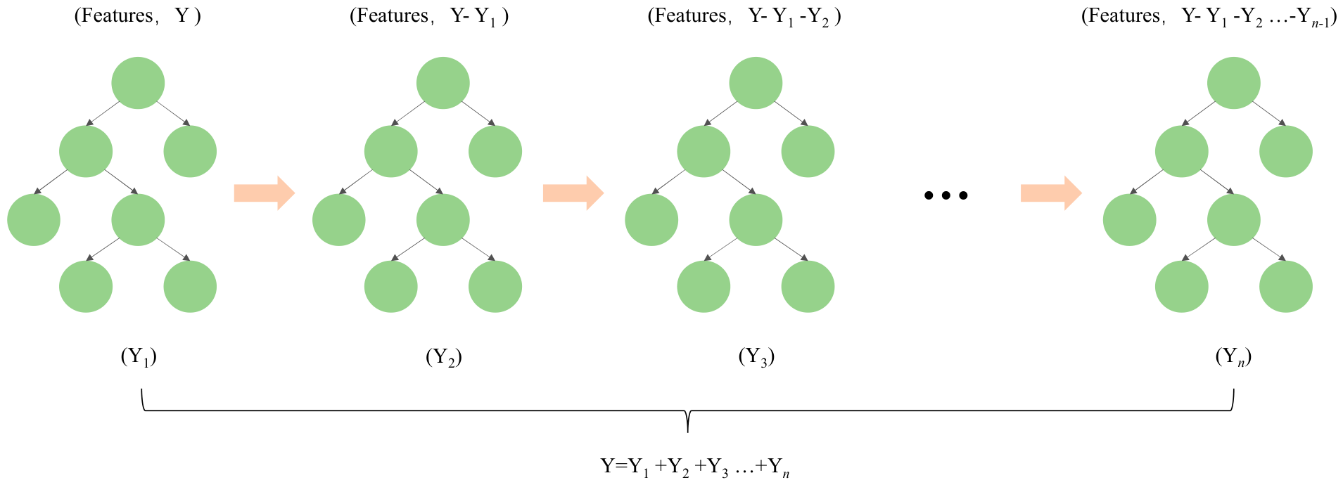
LightGBM (light gradient boosting machine) is a distributed gradient boosting framework [11] based on the decision tree algorithm. The basic structure of the gradient boosting decision tree (GBDT) [26] is a forest of decision trees. GBDT is used as an ensemble model, and predictions are made by adding the results of all subtrees. GBDT generates the entire forest by generating decision subtrees one at a time. The process of generating a new subtree consists of constructing a new subtree using the residuals between the sample labeled values and the current forest predictions. LightGBM learns by boosting algorithms [27], which are reinforced by a weak learner and trained by weighting. The training process is stepped, with the base models being trained one by one in order (the implementation can be made parallel), and the training set of the base models being transformed a certain way each time according to some strategy [12,13,14]. Finally, a linear synthesis of all base model predictions produces the final prediction.

In the process of constructing the gradient boosting tree, new subtrees are constructed one at a time using the residuals of the sample labeled values and the current forest predictions to ensure that each subtree positively affects the overall prediction effect, as illustrated in Figure 1. In the case of m decision trees, the final prediction F is the set of outputs from all subtrees, defined as in Equation (1).

$$F_m\left(x_i\right)={\displaystyle \sum _{k=1}^m{f}_k\left(x_i\right)}=F_{m-1}\left(x_i\right)+f_m\left(x_i\right)$$

(1)

where $F_{m-1}\left(x_i\right)$ is the cumulative prediction from the first $m-1$ sub-models, and $f_m\left(x_i\right)$ is the prediction from the newly built $m-th$ subtree. This formulation embodies the essence of “boosting”, where the model sequentially improves by combining the outputs of multiple weak learners.

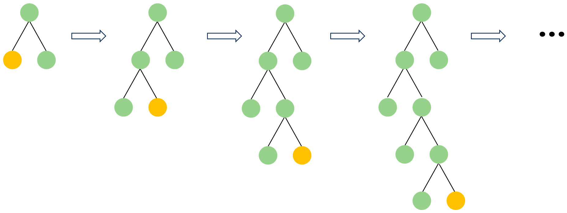
In order to meet the industry’s demand to shorten the computation time of models, the design idea of LightGBM has two main points: (1) to reduce the memory usage for data and ensure that a single machine can use as much data as possible without sacrificing speed. (2) to reduce the communication cost, improve the efficiency of the multi-machine when it is parallel, and realize linear acceleration in computation. It follows that LightGBM was originally designed to provide a fast and efficient data science tool with low memory consumption, high accuracy, and support for parallel and large-scale data processing. Figure 2 shows a schematic diagram of leaf growth in LightGBM.

The gradient boosting process, LightGBM, uses first- and second-order gradient information for optimization. Newton’s method is used to optimize the loss function, and gradient pruning is used to avoid overfitting and improve generalization performance.

$${\omega }_{t+1}={\omega }_t-{\displaystyle \frac{g_t}{h_t+\lambda }}$$

(2)

where ${\omega }_t$ denotes the weight of the t-th iteration, $g_t$ denotes the gradient of the t-th iteration, $h_t$ denotes the Hessian matrix of the t-th iteration, and $\lambda$ denotes the regularization parameter.

To deal with the excessive number of split points, LightGBM uses a histogram algorithm. As shown in Figure 3, the histogram of a leaf can be obtained by taking the difference between the histogram of its parent node and that of its sibling. This allows LightGBM, after constructing the histogram of a leaf, to obtain the histogram of its sibling leaf at a very low cost, which can be doubled in speed.

The following equation is an expression for the histogram $H_j$:

$$H_j=\{(v_i,g_i,h_i)|q_j^l\le v_i\le q_j^r\}$$

(3)

where $H_j$ denotes the histogram of the jth feature, $q_j^l$ and $q_j^r$ denote the left and right demarcation points of the jth feature, $v_i$ denotes the value of the ith sample on the jth feature, and $g_i$ and $h_i$ denote the gradient and Hessian matrix of the ith sample, respectively. LightGBM uses a histogram-based decision tree algorithm that discretizes continuous features into a number of histograms and then computes the information gain of the features on the histograms, thereby reducing time complexity and memory consumption.

To solve the problem of excessive sample size, LightGBM uses the gradient-based one-side sampling (GOSS) algorithm. By definition, instances with large gradients have a greater impact on information gain. Therefore, samples with large gradients (predetermined thresholds or the highest percentile) should be retained, and samples with small gradients should be randomly removed. This approach gives more accurate results than random sampling at the same sampling rate, especially when the range of information gain is large. On the one hand, the algorithm focuses more attention on undertrained samples, and on the other hand, it prevents the sampling from affecting the original data distribution too much by multiplying the weights.

To deal with the excessive number of features, LightGBM uses the exclusive feature bundling (EFB) algorithm. EFB reduces the feature dimensions by feature bundling (which is actually a dimensionality reduction technique) to improve computational efficiency. The features to be bundled are mutually exclusive (one feature with a zero value and one with a non-zero value) so that no information is lost when two features are bundled. When two features are not completely mutually exclusive (in some cases, both features have non-zero values), the degree to which the features are not mutually exclusive can be measured by a metric called the conflict ratio. If this value is small, it is possible to bundle two features that are not completely mutually exclusive without affecting the final accuracy.

LightGBM does not segment data vertically. Each machine has the complete data of the training set, and after obtaining the optimal partitioning scheme, the partitioning can be performed locally, reducing unnecessary communication. For cases where the amount of data is particularly large and the number of features is also particularly large, voting parallelism can be used. Voting parallelism reduces the communication cost by merging histograms of only some features by voting, which is mainly optimized for the bottleneck that the communication cost of merging data is relatively high when the data is parallel [15].

LightGBM was selected as the prediction framework in this study for two main reasons. First, compared with widely used alternative ensemble methods documented in the original benchmarks [11], LightGBM provides distinct technical advantages for the present problem: the gradient-based one-side sampling (GOSS) algorithm reduces memory consumption during training; the exclusive feature bundling (EFB) algorithm efficiently handles the 41-dimensional feature space considered here; and the gradient boosting approach reduces the test mean squared error by approximately 20–30% compared with traditional bagging-based ensemble methods. These features make LightGBM particularly well-suited for the 7500-case dataset adopted in this work.

Second, the present formulation enables the prediction of steady-state outputs at each time step from the current operating conditions and physical state. By including “time” as an engineered input feature alongside the other 37 physical parameters, the model effectively learns the time-dependent trajectory; the SHAP analysis presented in Section 3.2 confirms that time is the most influential feature for all four prediction targets.

A well-established performance metric system facilitates model tuning, optimization, and prediction performance improvement. Therefore, in order to train an artificial intelligence prediction model with better performance and robustness, it is necessary to explore the evaluation effect of various metrics on the time-series prediction of complex operating condition parameters in the model training process. The core evaluation metrics include the prediction speed and prediction accuracy of the model. The mean squared error (MSE) evaluates the accuracy by calculating the mean of the sum of the squares of the differences between each predicted and ground-truth value, indicating the extent to which the predicted and ground-truth values differ. The smaller the value, the better the model performs, and the closer the predicted value is to the ground-truth value. The formula is as follows:

$$MSE={\displaystyle \frac{1}{n}}{\displaystyle \sum _{i=1}^n{(y_i-{\widehat{y}}_i)}^2}$$

(4)

where $y_i$ is the ground-truth value, ${\widehat{y}}_i$ is the predicted value, and n is the sample size.

The coefficient of determination ($R^2$) allows you to better compare the performance of the model on data of different sizes. The closer the $R^2$ value is to 1, the better the fit and the better the model. The evaluation of error by $R^2$ is realized by the ratio of MSE to variance (Var). The formula is as follows:

$$R^2=1-{\displaystyle \frac{{\displaystyle \sum _{i=1}^n}{\left(y_i-{\widehat{y}}_i\right)}^2}{{\displaystyle \sum _{i=1}^n}{y}_i-{\overline{y}}_i^2}}=1-{\displaystyle \frac{MSE}{Var}}$$

(5)

where ${\overline{y}}_i$ is the mean of the ground-truth values.

In recent years, AI models have been widely used, but in most cases, AI models are used as “black boxes”, i.e., they are fed with model inputs and receive model outputs. For safety-critical fields such as nuclear power plant safety analysis, the “black-box” nature of AI models poses a potential risk to the reliability of analysis results. Therefore, to better understand the working mechanism of models and to increase people’s trust in the models, the study and analysis of model interpretability will help [16].

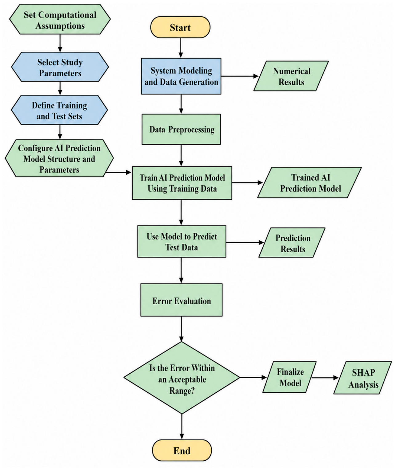
SHAP interprets the output of any machine learning model in a unified way. The core idea is to view the prediction of the state as the result of a game between event parameters. Each event parameter can be considered as a participant, and the predicted outcome of the event model is the total value produced by the cooperation of these participants [28]. The SHAP method attempts to assign a Shapley value to each event parameter, which indicates the contribution of that parameter to the results of the mode prediction [29]. The overall prediction framework is illustrated schematically in Figure 4, providing a clear overview of the prediction approach.

In the event of a minor break in the reactor coolant system piping or components connected to it, the rate of coolant loss exceeds the normal makeup capacity of the coolant makeup system. This type of coolant loss accident is referred to as a small-break loss-of-coolant accident (SBLOCA). An SBLOCA loss-of-water incident is characterized by a low rate of system coolant loss, a gradual depressurization rate, a phase separation between the vapor and liquid phases in the system, and a significant impact of heat conduction in the steam generator on the depressurization process. Furthermore, the SBLOCA employed a three-phase spray release, re-flooding, and long-term core cooling strategy, with no re-flooding phase. This approach resulted in a distinct pressure plateau at pressures slightly higher than the secondary-side heat-trap pressure.

A total of 7500 SBLOCA calculation cases were executed. Each RELAP5 simulation produced two types of files: an output file with the “.o” extension and a restart binary file with the “.r” extension. For a single case, the output file size was approximately 131.7 MB (134,833 KB), and the restart file size was approximately 168.6 MB (172,628 KB). Thus, the total raw data generated from all 7500 cases amounted to 7500 × (131.7 + 168.6) MB ≈ 2,252,250 MB, or about 2.15 TB. Given the large size of the output and restart files, which were impractical to process directly, and because a considerable portion of their content was not directly relevant to algorithm training, selected feature parameters were extracted for further analysis. In this study, the RELAP5 output interval was set to 1 s, and data from 1 to 500 s were exported into Excel files. Through sensitivity analysis, 41 parameters were identified as characteristic features.

A total of 37 input parameters and 4 output parameters were identified. SBLOCA was operated 7500 times (in groups) under accident conditions, and 500 data points were extracted for each operating mode, resulting in a total of 3,750,000 data points (in millions). In light of the accident process of the SBLOCA water loss accident and the related nuclear power plant system response, it can be posited that the parameters shown in

Table 2. Variables affecting water loss incidents in small breaks.

Input Parameter	Variable Name	Sl. No.
Core Power	Core Power	1
	Decay Power	2
Break	Break Area	3
	In-Containment Pressure at Break	4
	Break Discharge Coefficient	5
	Break Friction Coefficient	6
Safety Injection System (SIS)	ACC Initial Pressure	7
	ACC Initial Temperature	8
	ACC Volume	9
	ACC Water Volume	10
	ACC Trigger Pressure	11
	ACC Injection Pipeline Area	12
	ACC Injection Friction Coefficient	13
	ACC Local Resistance Coefficient at the Outlet	14
In-Containment Refueling Water Storage Tank (IRWST)	Initial Pressure	15
	Initial Temperature	16
	Water Tank Volume	17
	Trigger Pressure	18
	Injection Pipeline Area	19
	Injection Friction Coefficient	20
	Exit Loss Coefficient	21
ADS System	ADS1 Discharge Coefficient	22
	ADS2 Discharge Coefficient	23
	ADS3 Discharge Coefficient	24
	ADS4 Discharge Coefficient	25
	ADS1 Start Time	26
	ADS2 Start Time	27
	ADS3 Start Time	28
	ADS4 Start Time	29
	ADS1-3 Friction Coefficient	30
Core Makeup Tank (CMT)	Initial Pressure	31
	Initial Temperature	32
	CMT Volume	33
	CMT Trigger Pressure	34
	CMT Injection Pipeline Area	35
	CMT Injecting Friction Coefficient	36
	CMT Exit Loss Coefficient	37
Output Parameters	Peak Cladding Temperature	38
	Core Surface Temperature	39
	Pressurizer Water Level	40
	Primary Coolant Pressure	41

may be selected as the influencing variables of the accident.

The SBLOCA dataset comprised approximately three million data items for 6193 operating modes, with an average of 500 data items per operating mode. It recorded the values of key parameters for each second from 0 to 500 s after the accident. During the training of the machine learning model, the dataset is divided into two distinct subsets, with 90% of the data utilized for training and 10% reserved for validation. Furthermore, a dataset comprising 75 operating modes is employed for testing purposes, with the objective of demonstrating the model’s predictive capabilities across a range of operational scenarios. The inputs to the model comprise 37 parameters, including time, core power, break area, and so forth. The outputs are peak cladding temperature, core surface temperature, pressurizer water level, and primary coolant pressure. In contrast to neural networks, decision trees necessitate the calculation of information gain for each input to the output, resulting in a single variable per output. In the case of multiple output variables, each output variable must be trained separately. In the case of the SBLOCA, four output variables must be considered: peak cladding temperature, core surface temperature, pressurizer water level, and primary coolant pressure. Four decision tree models must be constructed in order to analyze the data.

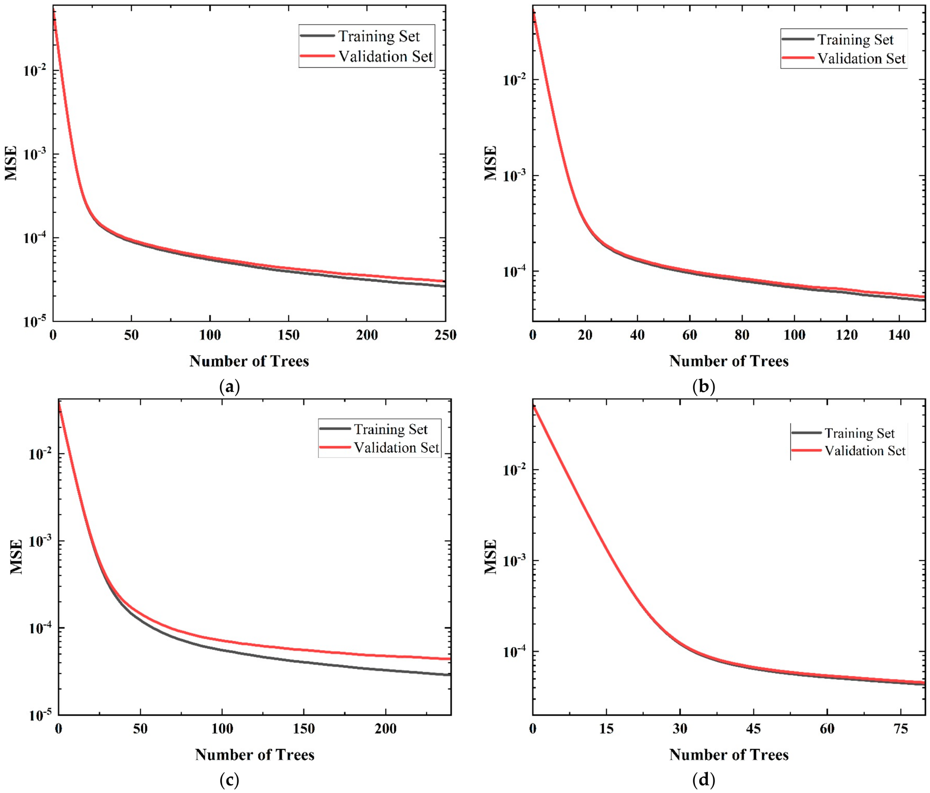
Prior to training the model, the dataset is normalized in order to facilitate the visualization of the model’s mean squared error, which exhibits a decreasing trend in relation to the gradient. Figure 5 illustrates the curve of mean squared error (MSE) with a gradient decrease during training for the LightGBM model for each of the four output models.

Figure 5a–d illustrate the impact of decreasing gradient on the prediction accuracy of the LightGBM regression model for peak cladding temperature, core surface temperature, pressurizer water level, and primary coolant pressure, respectively, in the SBLOCA test set. The black curve represents the results of the training set, while the red curve represents the results of the validation set. The distance between the black curve and the red curve on the vertical axis can be used to determine whether overfitting has occurred during the gradient descent. As illustrated in Figure 5a, the machine learning model of peak cladding temperature exhibits a gradual decline in the validation set MSE relative to the training set MSE as the decision tree reaches 200 trees. This phenomenon is accompanied by an increasing prevalence of overfitting. The machine learning model for the core surface temperature, as illustrated in Figure 5b, demonstrates a gradual separation of the two curves at 140 decision trees. In contrast, in the pressurizer water level machine learning model depicted in Figure 5c, the accuracy of the validation set is consistently inferior to that of the training set prior to the MSE curve becoming relatively smooth. Furthermore, the phenomenon of overfitting is invariably present. The primary coolant pressure machine learning model depicted in Figure 5d demonstrates a consistent match between the training set accuracy and the validation set accuracy during gradient descent, with minimal overfitting.

The hyperparameters of the LightGBM models were determined through a predefined hyperparameter search process. The search space adopted for model optimization is summarized in

Table 3. Hyperparameter search space.

Hyperparameter	Search Space	Description
Learning rate	0.01–0.20	Step size for gradient boosting
Number of trees (n_estimators)	50–300	Maximum number of boosting iterations
Maximum tree depth (max_depth)	3–12	Maximum depth of individual trees
Number of leaves (num_leaves)	31–2600	Maximum number of leaves in each tree
Minimum data in leaf (min_data_in_leaf)	10–100	Minimum number of samples per leaf
Feature fraction	0.6–1.0	Fraction of features used for each tree
Bagging fraction	0.6–1.0	Fraction of training samples used for bagging
Bagging frequency	1–10	Frequency of bagging
L1 regularization (lambda_l1)	0–1	L1 regularization coefficient
L2 regularization (lambda_l2)	0–1	L2 regularization coefficient

. Since four independent LightGBM models were developed for the four output variables, all models shared the same hyperparameter search space, while the optimal hyperparameter combination for each model was selected according to the validation performance. Once the optimal gradient has been selected, the accuracy of the trained models for different output parameters is displayed in

Table 4. Parameter list of the gradient boosting decision tree model for small-break accidents.

Output Parameters	Number of Trees	Number of Leaves	Mean Squared Error MSE (Normalized)
Peak Cladding Temperature	156	385	0.00061
Core Surface Temperature	153	326	0.00074
Pressurizer Water Level	125	2300	0.0014
Primary Coolant Pressure	84	326	0.00069

. The mean squared error of the four gradient boosting decision tree models on the normalized validation set is less than 0.01, and the corresponding coefficients of determination are all greater than 0.99.

The following software tools were used in this study: RELAP5/MOD3.3 for nuclear reactor transient simulation; Python 3.10 for data preprocessing; and LightGBM 4.6.0 for the gradient boosting decision tree regression model.

3. Results and Discussion

3.1. LightGBM Prediction Performance

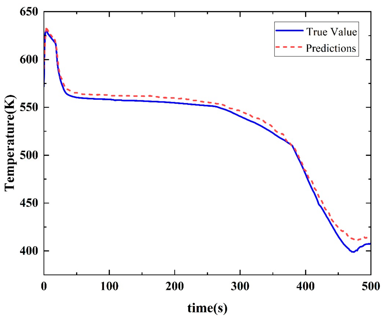
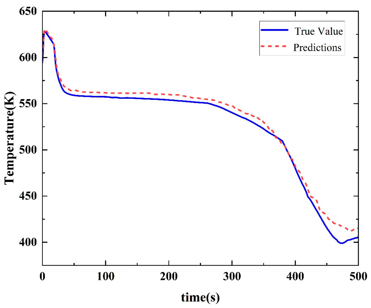
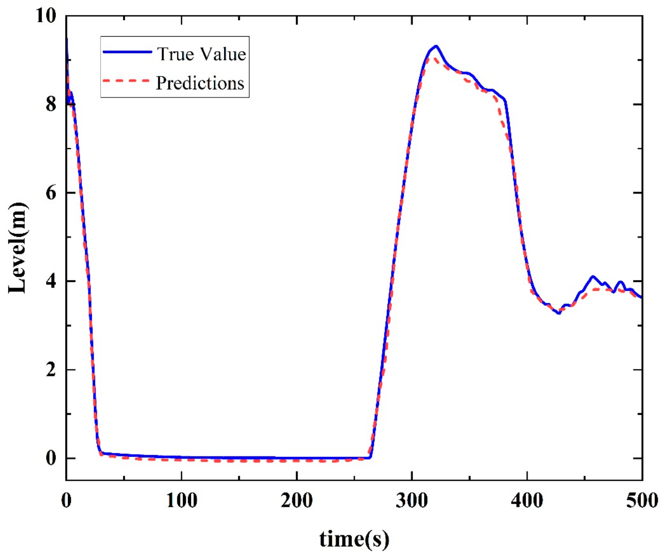
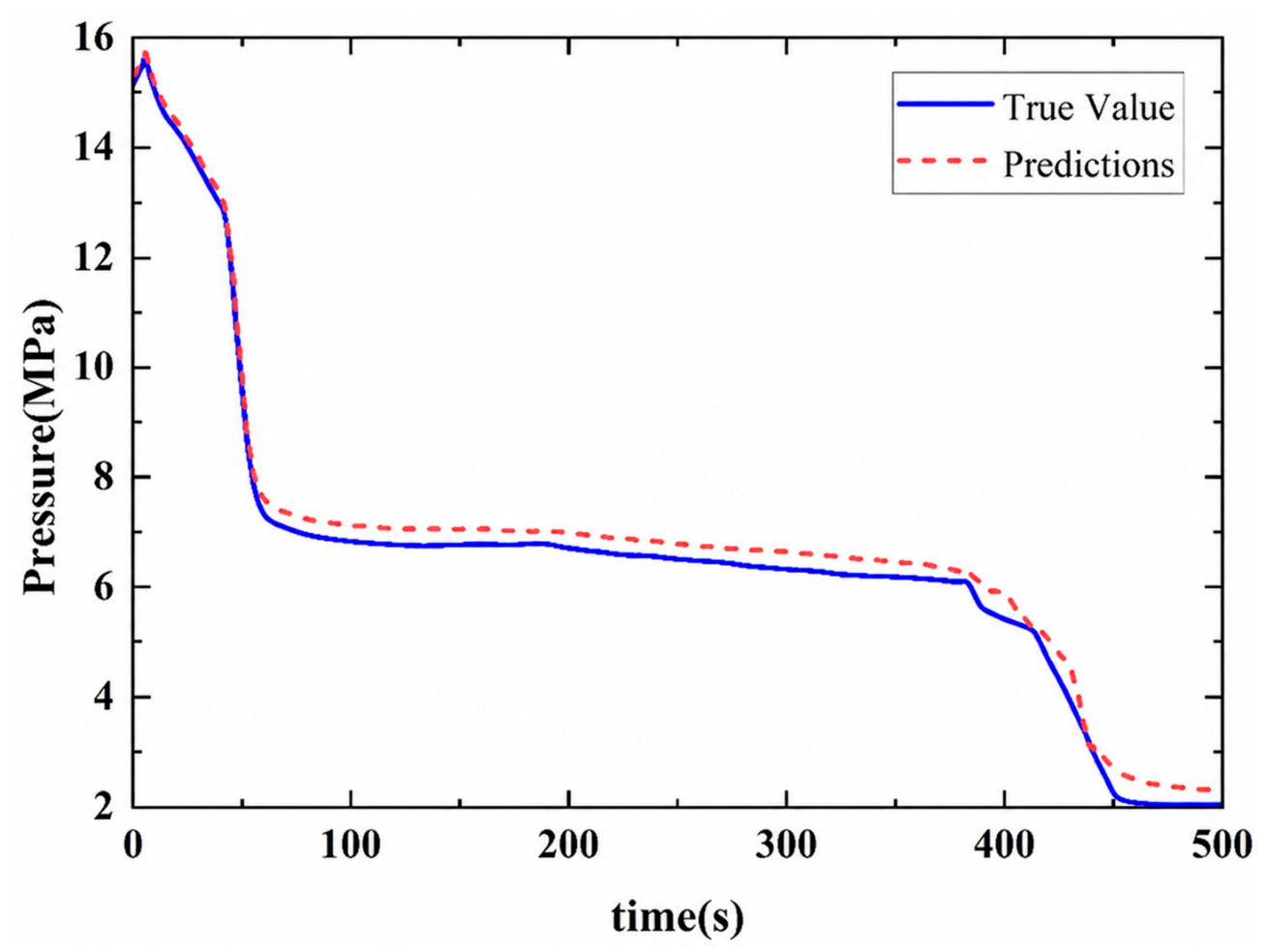
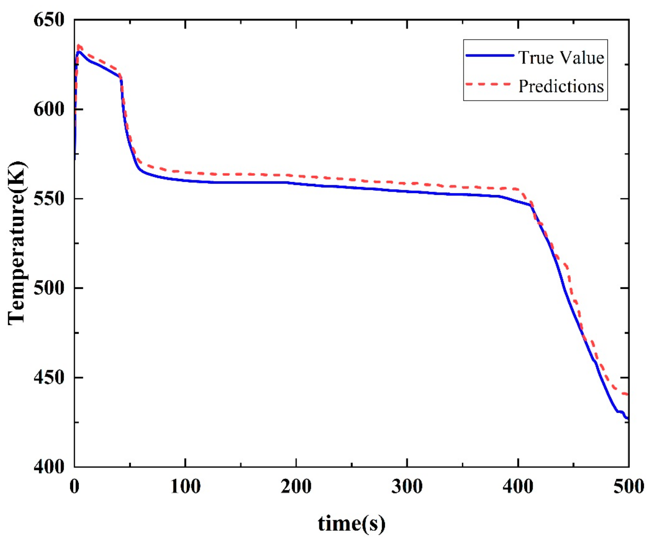
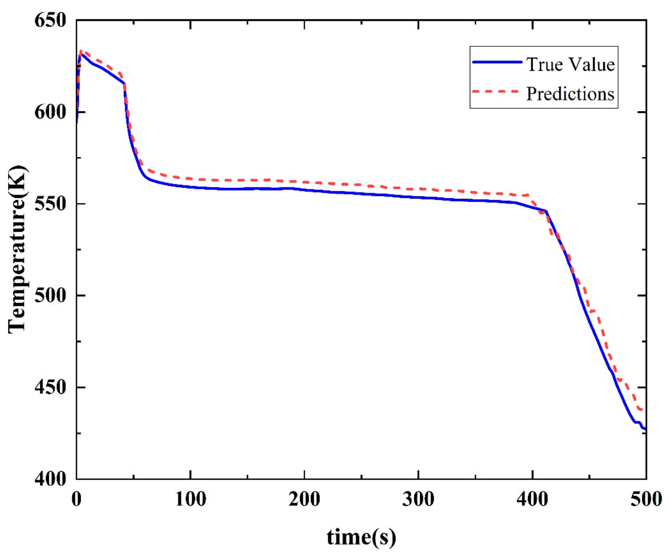
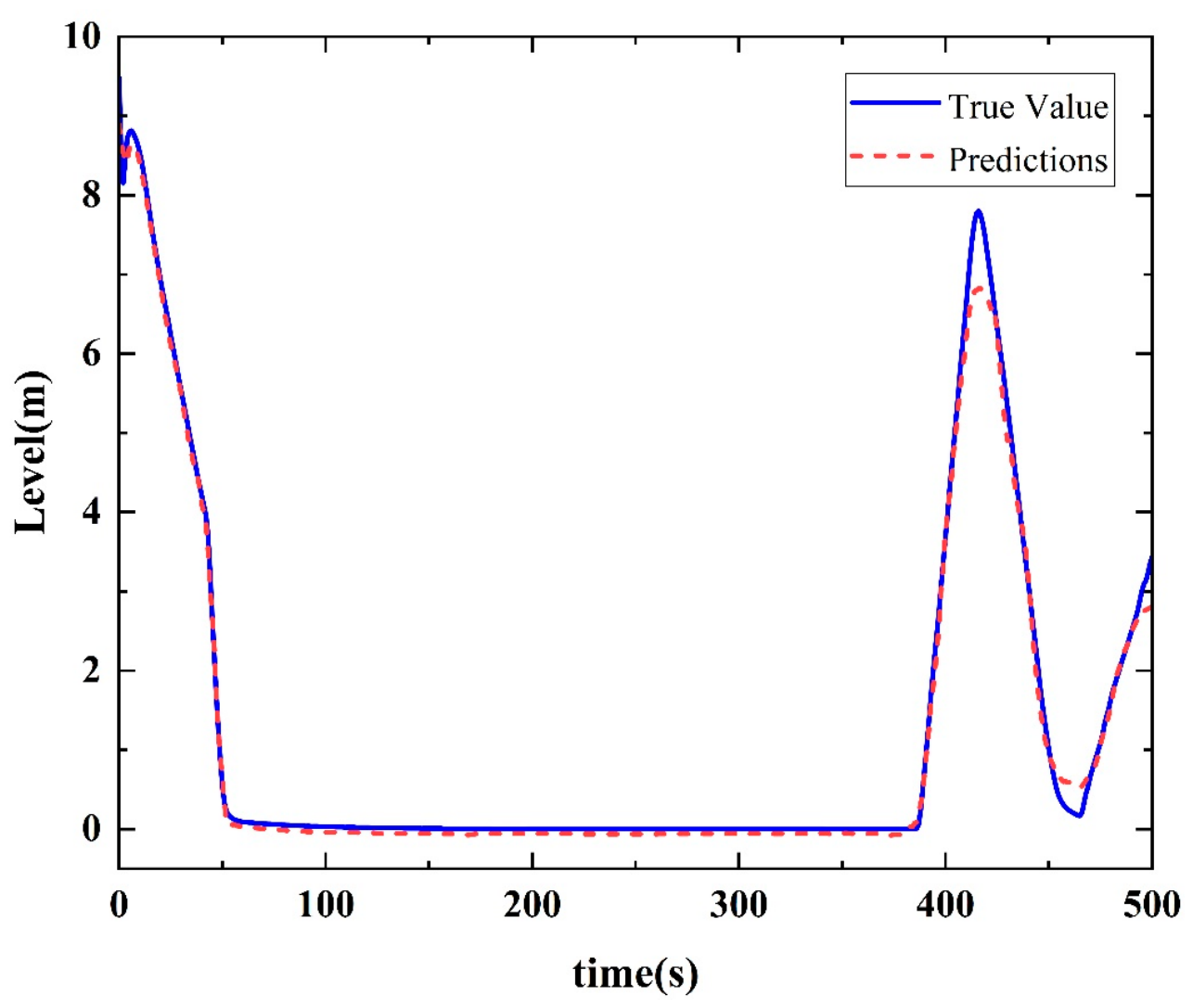
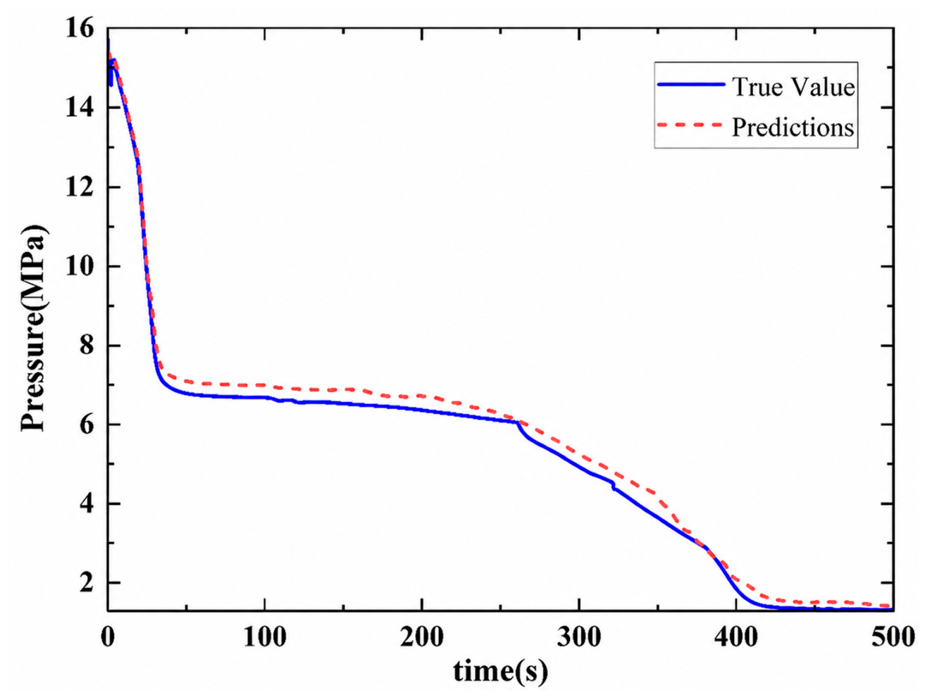
The results of the trained gradient boosting decision tree model for individual operating modes of peak cladding temperature, core surface temperature, pressurizer water level, and primary coolant pressure in the SBLOCA test set are presented in Figure 6, Figure 7, Figure 8 and Figure 9.

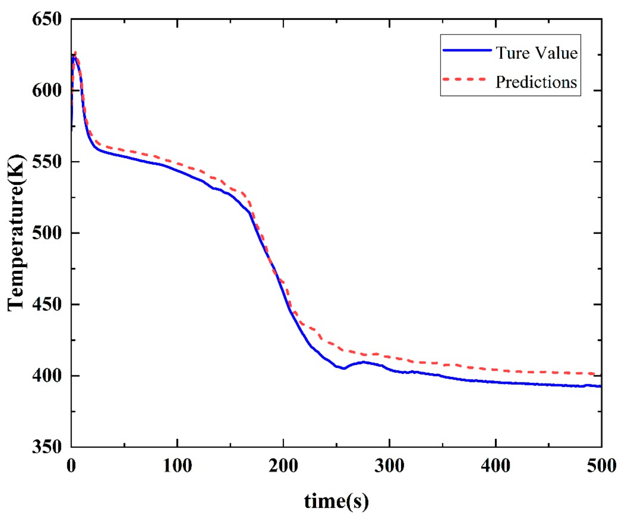
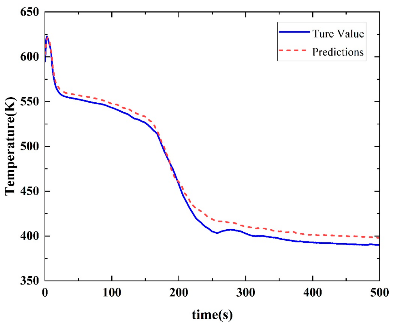
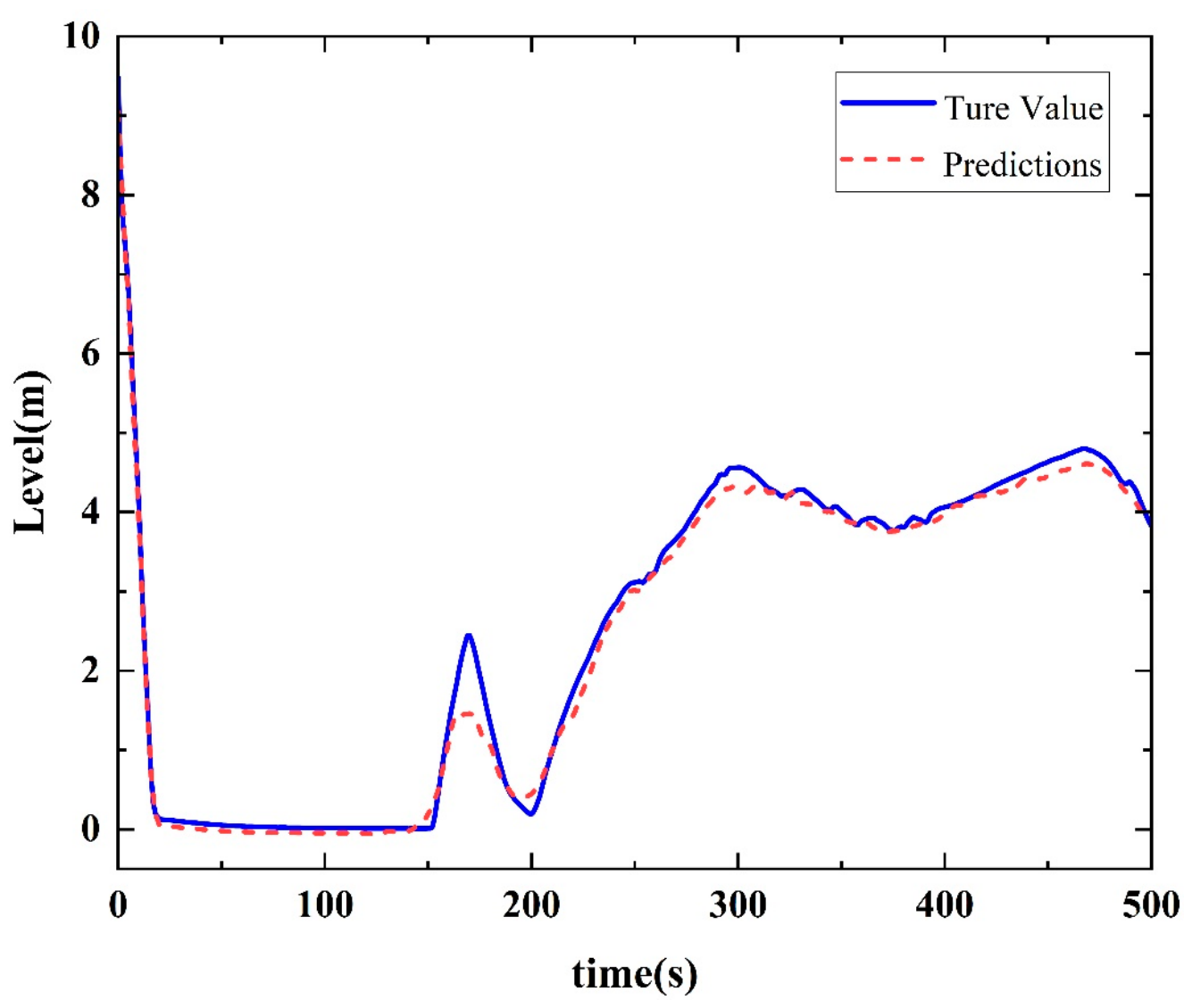
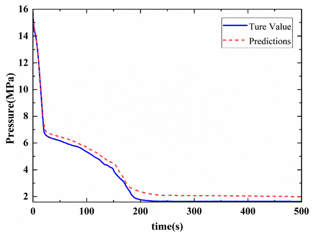
Figure 6, Figure 7, Figure 8 and Figure 9 illustrate the outcomes of the trained gradient boosting decision tree model for the operating mode prediction for number 54 in the training set in comparison to the ground-truth value over time. The horizontal axis represents the temporal dimension, specifically the time (in seconds) elapsed. The vertical axis represents the individual output parameters. The temperature is expressed in Kelvin, while the pressure is expressed in megapascals (MPa). The blue curve represents the true value, while the red curve represents the predicted value of the regression model at each point in time. The predictions for all four outputs are in close alignment with the true values and accurately reflect the trend of the outputs over time. In this set of operational modes, peak cladding temperature and core surface temperature increased sharply to 630 K following the accident and then decreased rapidly within 40 s. This was followed by a slow decrease in the interval from 40 to 360 s, after which the rate of decrease became faster at 380 s. The temperature then decreased to the lowest point of about 400 K after 80 s, followed by slight fluctuations. Following the accident operating mode, the pressurizer water level exhibited a precipitous decline to zero within 20 s. At approximately 260 s, the pressurizer water level commenced a rapid ascent, reaching a peak at 310 s and subsequently declining at a rapid pace before stabilizing and entering a prolonged period of cooling. Following the incident, in the operating mode, a sharp decline in primary coolant pressure was observed, reaching a nadir after 40 s. Thereafter, the rate of decline slowed until it leveled off after 480 s.

Figure 10, Figure 11, Figure 12 and Figure 13 illustrate that the gradient boosting decision tree model exhibited comparable accuracy in predicting the four output variables in operating mode 35.

In operating mode 35, the peak cladding temperature and core surface temperature undergo a second rapid decline at an earlier time point than in operating mode 54, reaching a plateau at 300 s. The changes in the pressurizer water level were markedly distinct from those observed in operating mode 54. Following the accidental activation of operating mode, the pressurizer water level exhibited a precipitous decline to zero within approximately 160 s. Subsequently, the pressurizer water level exhibited minor fluctuations, followed by a rapid ascent to a peak. This peak was reached within 300 s, after which the pressurizer water level began to fluctuate and stabilized. It then entered a long-term cooling phase.

In both operational modes, the gradient boosting decision tree demonstrated the capacity to target and accurately predict outcomes, despite the disparate trends observed in the four outputs.

Figure 14, Figure 15, Figure 16 and Figure 17 illustrate the predictive outcomes for a second set of operational modes (46). The gradient boosting decision tree model also demonstrated accurate prediction performance for the four output variables.

Table 5. Quantitative analysis of individual working conditions of the model.

Case Number	Output Parameters	${\mathit{R}}^2$	Computing Speed (Single Data, Seconds)
54	Peak Cladding Temperature	0.9890	$3.72 \times {10}^{-4}$
	Core Surface Temperature	0.9843	$1.73 \times {10}^{-4}$
	Pressurizer Water Level	0.9979	$2.56 \times {10}^{-4}$
	Primary Coolant Pressure	0.9850	$1.65 \times {10}^{-4}$
35	Peak Cladding Temperature	0.9877	$3.72 \times {10}^{-4}$
	Core Surface Temperature	0.9877	$1.73 \times {10}^{-4}$
	Pressurizer Water Level	0.9909	$2.56 \times {10}^{-4}$
	Primary Coolant Pressure	0.9832	$1.65 \times {10}^{-4}$
46	Peak Cladding Temperature	0.9829	$3.72 \times {10}^{-4}$
	Core Surface Temperature	0.9820	$1.73 \times {10}^{-4}$
	Pressurizer Water Level	0.9943	$2.56 \times {10}^{-4}$
	Primary Coolant Pressure	0.9956	$1.65 \times {10}^{-4}$

presents the prediction accuracy and computational speed for the three operating modes.

As illustrated in Table 5, while the four output parameters in each of the three operating modes exhibit divergent temporal trends, the trained gradient boosting decision tree consistently generates accurate predictions. The coefficients of determination are all greater than 0.98, indicating a satisfactory fit to the key output parameters. Furthermore, the pressurizer water level and primary coolant pressure parameters exhibit a peak value that differs depending on the time point of coolant makeup in the operational mode. For cases where no coolant makeup is activated within 500 s after the accident, the pressurizer water level drops sharply to 0 and remains stable, leading to higher data complexity and noise. Nevertheless, when the coefficients of determination are incorporated into the overall fit, the resulting value remains high. The model was able to accurately predict the trend of the four parameters over time, with the loss function remaining within 0.03 throughout. Furthermore, the prediction time for each operating mode output parameter was less than $4 \times {10}^{-4}$ s.

Although various advanced machine learning methods have been developed for regression and domain adaptation problems, their applicability depends strongly on the characteristics of the target dataset and prediction objectives. Methods such as asynchronous joint distribution alignment (AJDA) mainly focus on domain adaptation problems, where the objective is to reduce distribution discrepancies between different domains and improve model transferability under changing data distributions. In contrast, the objective of this study is to establish a high-efficiency surrogate model for predicting multiple safety parameters under SBLOCA conditions based on RELAP5-generated transient datasets. The training and testing data in this work are obtained from the same simulation framework, and therefore, the primary challenge is the accurate representation of nonlinear relationships between thermal–hydraulic parameters rather than cross-domain feature alignment.

Compared with deep learning-based methods, gradient boosting decision tree models generally require fewer training samples and provide strong capability in handling structured engineering datasets with nonlinear interactions among variables. Furthermore, LightGBM offers advantages in computational efficiency and model convergence, which are important requirements for real-time applications in nuclear power plant full-scope simulators. Although domain adaptation methods such as AJDA provide valuable approaches for improving model robustness under different data distributions, their advantages are mainly reflected in cross-domain prediction tasks rather than transient parameter prediction within a consistent simulation environment. Future studies will further investigate the integration of domain adaptation techniques and hybrid learning frameworks to improve the generalization capability of nuclear transient surrogate models under broader operating conditions.

LightGBM’s leaf-wise growth strategy tends to grow deeper trees compared to level-wise growth, which can lead to overfitting on noisy training samples if the number of leaves and tree depth are not properly controlled. In this work, overfitting is mitigated through: (1) early_stopping_rounds = 50 to halt training when the validation set MSE fails to improve; (2) min_data_in_leaf ≥ 10 to prevent leaves from capturing too few samples; (3) lambda_l1 = 0.1 and lambda_l2 = 0.1 to regularize the loss function; and (4) feature_fraction = 0.6–1.0 and bagging_fraction = 0.6–1.0 to introduce randomness and reduce overfitting to specific feature combinations.

3.2. SHAP-Based Feature Importance Analysis

SHAP is a method for interpreting the results of machine learning models. It is primarily used to create dependency graphs, including swarm, bar, force, and feature graphs.

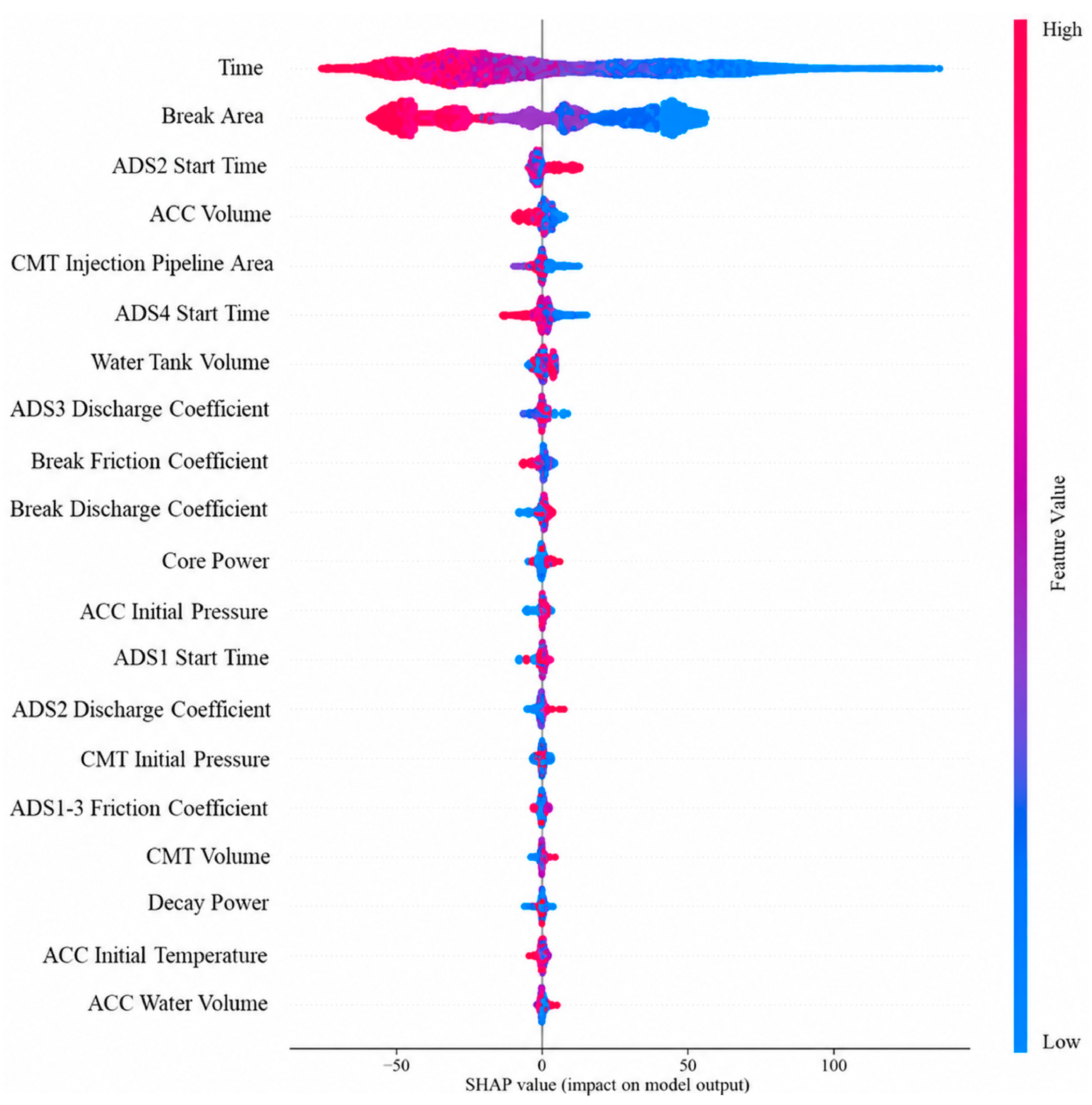
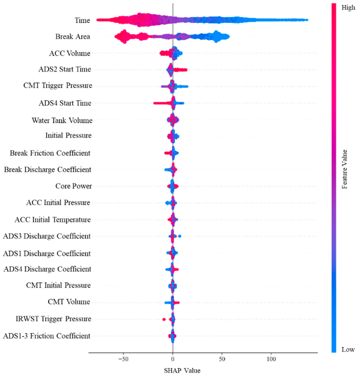
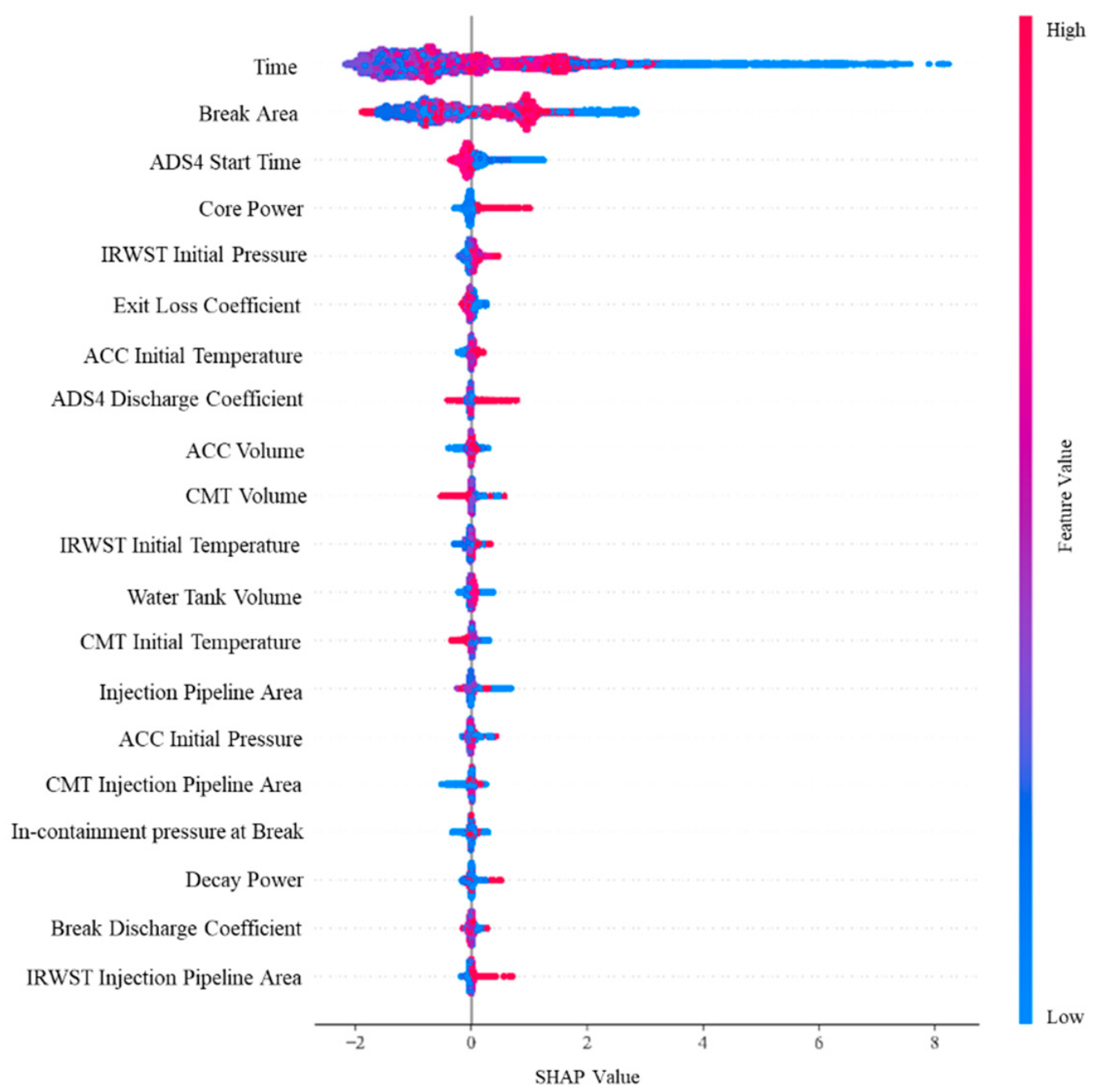
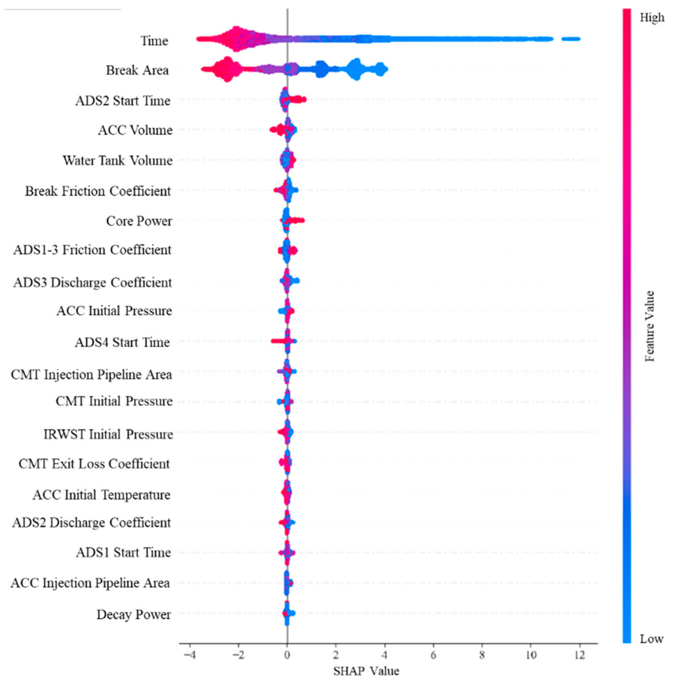
A beeswarm plot is an information-dense summary that illustrates the impact of the most salient features in a dataset on the model’s output. Each instance of interpretation within the SHAP beeswarm graph is represented by a point on each feature map. The X position of the point is contingent upon the SHAP value of the feature. The dots are arranged in a linear sequence along each feature row to illustrate the density of the data. The graph is composed of rows, each representing a feature. The horizontal coordinate represents the SHAP value. The features are presented in descending order of the mean absolute value of SHAP. Wide areas indicate the presence of a significant number of samples. The use of a dot to represent a sample and the color of the dot to indicate the original value of the feature is a standard practice in this field. The color red is indicative of a larger value for the feature in question, whereas the color blue is indicative of a smaller value.

A SHAP chart can be conceptualized as a type of ranking chart that depicts the relative importance of features. Figure 18, Figure 19, Figure 20 and Figure 21 illustrate the SHAP beeswarm plots for the peak cladding temperature model, the core surface temperature model, the pressurizer water level model, and the primary coolant pressure model, respectively. The horizontal coordinate is the SHAP value, and the feature ordering is based on the absolute mean of the SHAP values.

As illustrated in Figure 18, Figure 19, Figure 20 and Figure 21, time is the most crucial factor in all four models, exerting the most significant influence on the objective function. The change in time is inversely proportional to all four objective functions. In terms of horizontal distribution, the samples of features across time are more dispersed, in accordance with the distribution of time in the dataset, which was sampled from 0 to 500 s. The break size is the most influential factor in the objective function, with the exception of time. As the break size diminishes, the peak cladding temperature, core surface temperature and primary coolant pressure all increase. Nevertheless, the size of the break is no longer inversely related to the pressurizer water level. This is due to the fact that some of the samples in the dataset had water poured into them after the accident to achieve prolonged cooling. Consequently, the effect of break size on the results cannot be judged intuitively.

The peak cladding temperature is influenced by a number of factors, including the ADS2 start time, ACC volume, CMT injection pipeline area, and ADS4 start time. It is evident from Figure 18 that the longer ADS2 is operational, the higher the peak temperature, and the longer ADS4 is operational, the lower the peak temperature. Furthermore, other variables, such as the ACC water volume and the initial temperature, contribute only marginally to the observed effect on the model output. However, it is also possible to observe the magnitude of the feature values in relation to the output from the beeswarm plots. Although the effects account for a relatively small percentage, their influence on the peak temperature is not negligible and still has a positive or negative effect.

When the model output is the core surface temperature, it can be observed from Figure 19 that the influence of the ADS1-3 friction coefficient and the IRWST trigger pressure on the results is almost equal to zero. It can be observed that the output of the model is largely independent of the magnitude of the feature values of the friction coefficients of ADS1-3 and the triggering pressure feature values of IRWST.

Figure 20 illustrates the distribution of key features influencing the prediction of the pressurizer water level and their respective contributions. Consistent with other models, time remains the most influential feature. Notably, the impact pattern of break size on the pressurizer water level differs from other parameters, as it does not exhibit a simple negative correlation. This is because, during the later stages of an SBLOCA, the activation of the safety injection system introduces water into the primary circuit, leading to a recovery in liquid level. Consequently, the influence of the break size is modulated by this water injection behavior.

Figure 21 presents the SHAP analysis results for the primary coolant pressure model. Time and break size are again the dominant factors. The break size shows a negative correlation with pressure, which aligns with thermal–hydraulic principles—smaller breaks lead to slower system depressurization. Additionally, the start-up timing and depressurization coefficients of the ADS significantly influence the pressure curve, particularly early-stage ADS activation, which accelerates system pressure reduction. In contrast, features such as the IRWST trigger pressure contribute minimally to pressure prediction, as their role is primarily relevant during long-term cooling phases and has limited impact on short-term pressure dynamics.

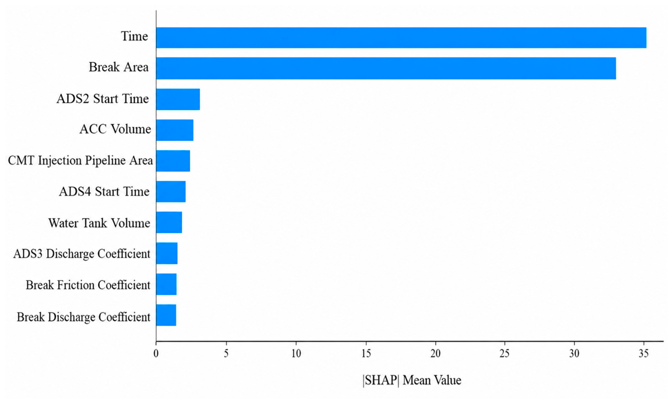
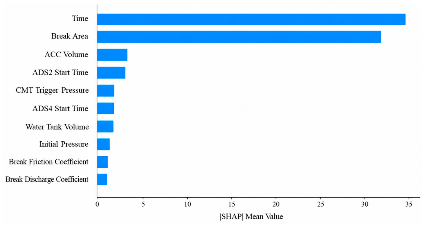
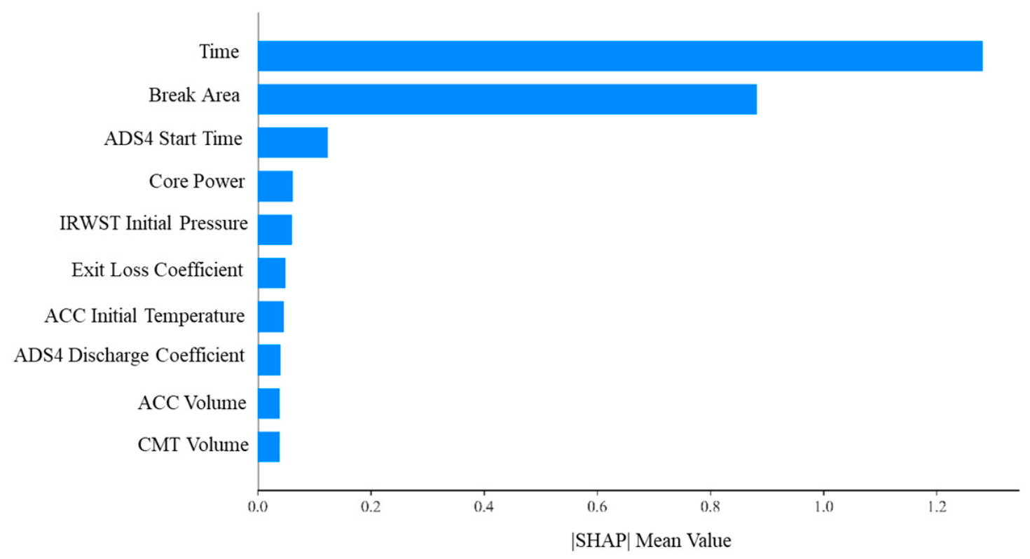
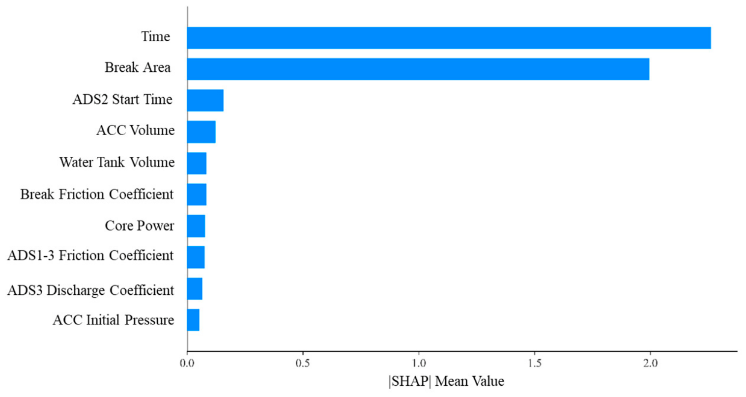
Figure 22, Figure 23, Figure 24 and Figure 25 illustrate the mean bar plots for the four models. The bar chart is generated by calculating the mean absolute value of the SHAP values. The bar chart is sorted by taking the absolute mean of the SHAP values, and the resulting sorting is identical to that of the beeswarm chart.

The SHAP mean bar plots in Figure 22, Figure 23, Figure 24 and Figure 25 systematically elucidate the dominance of time and break size in predicting all four key parameters by quantifying feature importance. This predominance stems from their direct determination of the physical progression of accident evolution and initial boundary conditions. The consistent ranking across these charts not only validates the LightGBM model’s ability to capture core physical mechanisms in nuclear power plant accident responses but also highlights the charts’ transformative role in converting “black-box” models into interpretable engineering tools. By revealing the differential influence of ADS system parameters on temperature and safety injection system parameters on liquid level, these visualizations directly map to intervention priorities of subsystems in practical accident management. This provides a data-driven foundation for rapid identification of key control variables and optimization of emergency operation sequences, demonstrating the value of AI models in achieving “physics-informed data fusion” within complex industrial scenarios.

3.3. Discussion of SHAP-Based Feature Importance

The consistency of SHAP results across different operating conditions further demonstrates the robustness of the proposed LightGBM framework. Although different SBLOCA scenarios exhibit different transient responses due to variations in boundary conditions and safety system activation sequences, time and break size consistently remain the dominant variables for all four prediction targets. This observation is consistent with the physical characteristics of accident progression. Time represents the evolution process of the accident, including coolant inventory loss, system depressurization, heat transfer degradation, and recovery through safety injection. Therefore, it directly determines the transient state of the reactor system. Break size determines the coolant discharge rate and strongly influences primary system pressure reduction, coolant inventory variation, and core cooling capability, resulting in its significant contribution to temperature, pressure, and water level predictions.

The contributions of safety system-related parameters also provide meaningful physical insights. For example, ADS activation timing affects the depressurization process and influences the conditions for accumulator and safety injection system operation. Therefore, ADS-related parameters show noticeable impacts on peak cladding temperature and primary coolant pressure predictions. Similarly, ACC volume and CMT injection parameters affect the available emergency coolant inventory and contribute to the prediction of the thermal response during the accident. Although some parameters exhibit relatively lower SHAP values, their effects remain physically meaningful because they influence specific stages of accident development rather than the overall transient evolution. The agreement between SHAP interpretation and thermal–hydraulic mechanisms indicates that the LightGBM model captures the essential physical relationships within the RELAP5-generated dataset rather than relying on accidental data correlations. This improves the reliability and engineering applicability of the proposed surrogate model for real-time nuclear power plant simulator applications.

4. Conclusions and Future Work

4.1. Conclusions

This study constructs a LightGBM surrogate model to rapidly predict four core safety parameters under pressurized water reactor small-break loss-of-coolant accident (SBLOCA) conditions. A total of 7500 representative operating cases are generated via parallel RELAP5 simulations to form the training dataset, and SHAP (Shapley additive explanations) is adopted to quantify the contribution of each input feature to model outputs. The main conclusions are summarized as follows.

(1) The proposed LightGBM model precisely predicts the transient curves of all four output parameters. For all test operating modes, the coefficient of determination R² exceeds 0.98, and the mean squared error stays below 0.002; the prediction error of the model is lower than 5%. The inference time for a single data point is less than $4\times {10}^{-4}$ seconds, boosting computational efficiency by roughly 32,500 times relative to native RELAP5 simulations.

(2) SHAP interpretability analysis verifies that time and break size serve as the two dominant features for all four prediction targets, matching the intrinsic thermal–hydraulic mechanisms during SBLOCA evolution. Safety system variables, including ADS activation timing and ACC water volume, exert secondary yet physically reasonable effects, whereas parameters such as the ADS1–3 friction coefficient have relatively trivial impacts and can be temporarily neglected.

(3) Uniform SHAP feature importance rankings under various working conditions further validate the robustness of the established framework. This proves that the LightGBM model learns fundamental physical correlations from RELAP5 simulation data instead of random coincidental data associations.

(4) The LightGBM surrogate model put forward in this paper provides a feasible, high-efficiency solution to speed up accident simulation calculation for full-scope nuclear power plant simulators. It has great potential to facilitate the construction of real-time decision support systems and operator training platforms for nuclear safety assessment.

However, several limitations of the present work should be acknowledged to properly delineate its scope of applicability.

(1) Static-tabular formulation. The time variable is included as an engineered input feature rather than through an explicit temporal recurrence mechanism. The present model, therefore, cannot represent short-timescale oscillations or feedback dynamics between consecutive time steps, and methods such as LSTM, GRU, and PINN are expected to provide complementary advantages for capturing such dynamics.

(2) In-distribution evaluation. All reported results are obtained on hold-out operating modes within the same RELAP5 simulation envelope. The robustness of the proposed model to genuinely out-of-distribution accident scenarios, such as multiple safety system failures or atypical transient initiators, has not been formally quantified and requires future systematic evaluation.

(3) In addition, while the present study does not include a formal sensitivity analysis under input perturbations, the consistency of the prediction performance across the three test operating modes (Case 35, Case 46, and Case 54) provides an indirect indication of the model’s robustness within the training envelope. The coefficient of determination R² varies by less than 0.02 across the three test cases for each of the four output parameters, suggesting that the prediction accuracy is not strongly sensitive to the specific combination of break size, ADS activation timing, and ACC water volume within the explored parameter range. However, this internal-consistency check does not substitute for a formal robustness evaluation under out-of-distribution conditions, and a systematic sensitivity analysis involving controlled noise injection, parameter perturbation beyond the training envelope, and cross-condition transfer is identified as an important direction for future work.

4.2. Future Work

Based on the limitations analyzed above, several promising directions are proposed for future improvement and extension of the present study.

(1) Physics-informed hybrid modeling. The integration of physics-informed constraints (e.g., conservation of mass, momentum, and energy) with the present LightGBM-based surrogate model will be explored to improve the physical consistency of the predictions and to enhance the extrapolation capability of the model beyond the training envelope.

(2) Sensitivity and robustness analysis under input perturbations. Controlled input perturbations will be adopted for comprehensive robustness tests: (a) different levels of Gaussian noise on raw features to record MSE and R²; (b) out-of-envelope parameter disturbances with other deviation magnitudes for break size and ACC volume to test extrapolation performance; (c) cross-condition validation between disjoint operating subsets to evaluate overall generalization. These tests will quantify the applicability domain of the LightGBM surrogate model.

(3) Uncertainty quantification. Uncertainty quantification methods, including Bayesian gradient boosting, quantile regression forests, and deep ensembles, will be incorporated to provide probabilistic predictions with associated confidence intervals, which are critical for risk-informed decision-making in safety-critical applications.

References

1. Jang, I.; Kim, Y.; Park, J. Investigating the Effect of Task Complexity on the Occurrence of Human Errors observed in a Nuclear Power Plant Full-Scope Simulator. Reliab. Eng. Syst. Saf. 2021, 214, 107704. [Google Scholar] [CrossRef]
2. Boring, R.L.; Agarwal, V.; Fitzgerald, K.; Hugo, J.; Hallbert, B. Digital Full-Scope Simulation of a Conventional Nuclear Power Plant Control Room, Phase 2: Installation of a Reconfigurable Simulator to Support Nuclear Plant Sustainability; U.S. Department of Energy, Office of Scientific and Technical Information: Oak Ridge, TN, USA, 2013. [Google Scholar]
3. Boring, R.L.; Agarwal, V.; Joe, J.C.; Persensky, J.J. Digital Full-Scope Mockup of a Conventional Nuclear Power Plant Control Room, Phase 1: Installation of a Utility Simulator at the Idaho National Laboratory; Idaho National Laboratory: Idaho Falls, ID, USA, 2012; pp. 1–2. Available online: https://www.researchgate.net/publication/265117822_Digital_Full-Scope_Mockup_of_a_Conventional_Nuclear_Power_Plant_Control_Room_Phase_1_Installation_of_a_Utility_Simulator_at_the_Idaho_National_Laboratory (accessed on 21 July 2026).
4. Ni, S.; Liu, M.; Gu, H. Modeling and validation of RELAP5 for natural circulation flow in a single PWR fuel assembly. Ann. Nucl. Energy 2021, 151, 107940. [Google Scholar] [CrossRef]
5. Saraswat, S.P.; Munshi, P.; Allison, C. Characteristics and linear stability analysis of RELAP5 two-fluid model for two-component, two-phase flow. Ann. Nucl. Energy 2021, 151, 107948. [Google Scholar] [CrossRef]
6. Racheal, S.; Liu, Y.; Ayodeji, A. Evaluation of optimized machine learning models for nuclear reactor accident prediction. Prog. Nucl. Energy 2022, 149, 104263. [Google Scholar] [CrossRef]
7. Ghoneim, O.; Dobias, P.; Romain, O. Survey of neural network optimization methods for sustainable AI: From data preprocessing to hardware acceleration. Mach. Learn. Appl. 2025, 22, 100762. [Google Scholar] [CrossRef]
8. Zubair, R.; Ullah, A.; Khan, A.; Inayat, M.H. Critical heat flux prediction for safety analysis of nuclear reactors using machine learning. In Proceedings of the 2022 19th International Bhurban Conference on Applied Sciences and Technology (IBCAST), Islamabad, Pakistan, 16–20 August 2022; IEEE: New York, NY, USA, 2022; pp. 314–318. [Google Scholar]
9. Tan, C.; Wang, B.; Li, J.; Chen, J.; Liang, B.; Zheng, S.; Han, R.; Tian, R.; Tan, S. Research on reactor power prediction of nuclear power plant based on multivariate optimization GRU model. Int. J. Adv. Nucl. React. Des. Technol. 2024, 6, 78–89. [Google Scholar] [CrossRef]
10. Mohanty, S.; Vilim, R. Physics-Infused AI/ML Based Digital-Twin Framework for Flow-Induced-Vibration Damage Prediction in a Nuclear Reactor Heat Exchanger; Argonne National Laboratory: Lemont, IL, USA, 2021. [Google Scholar]
11. Ke, G.; Meng, Q.; Finley, T.; Wang, T.; Chen, W.; Ma, W.; Ye, Q.; Liu, T.-Y. LightGBM: A Highly Efficient Gradient Boosting Decision Tree. Adv. Neural Inf. Process. Syst. 2017, 30. [Google Scholar]
12. Sun, X.; Liu, M.; Sima, Z. A novel cryptocurrency price trend forecasting model based on LightGBM. Financ. Res. Lett. 2020, 32, 101084. [Google Scholar] [CrossRef]
13. Cai, Z.; Huang, H.; Sun, G.; Li, Z.; Ouyang, C. Advancing Predictive Models: Unveiling LightGBM Machine Learning for Data Analysis. In Proceedings of the 2023 4th International Conference on Computer, Big Data and Artificial Intelligence (ICCBD+AI), Guiyang, China, 15–17 December 2023; IEEE: New York, NY, USA, 2023; pp. 109–112. [Google Scholar]
14. Wang, Y.; Chen, J.; Chen, X.; Zeng, X.; Kong, Y.; Sun, S.; Guo, Y.; Liu, Y. Short-Term Load Forecasting for Industrial Customers Based on TCN-LightGBM. IEEE Trans. Power Syst. 2021, 36, 1984–1997. [Google Scholar] [CrossRef]
15. Seyyedattar, M.; Zendehboudi, S.; Ghamartale, A.; Afshar, M. Advancing hydrogen storage predictions in metal-organic frameworks: A comparative study of LightGBM and random forest models with data enhancement. Int. J. Hydrogen Energy 2024, 69, 158–172. [Google Scholar] [CrossRef]
16. Lundberg, S.M.; Erion, G.; Chen, H.; DeGrave, A.; Prutkin, J.M.; Nair, B.; Katz, R.; Himmelfarb, J.; Bansal, N.; Lee, S.-I. From local explanations to global understanding with explainable AI for trees. Nat. Mach. Intell. 2020, 2, 56–67. [Google Scholar] [CrossRef] [PubMed]
17. Cheng, J.; Liu, J.; Chen, S.; Li, Y.; Wang, J.; Wang, F. A new method for safety classification of structures, systems and components by reflecting nuclear reactor operating history into importance measures. Nucl. Eng. Technol. 2022, 54, 1336–1342. [Google Scholar] [CrossRef]
18. Adamantiades, A.; Kessides, I. Nuclear power for sustainable development: Current status and future prospects. Energy Policy 2009, 37, 5149–5166. [Google Scholar] [CrossRef]
19. Burns, P.; Ewing, R.; Navrotsky, A. Nuclear Fuel in a Reactor Accident. Science 2012, 335, 1184–1188. [Google Scholar] [CrossRef] [PubMed]
20. Zou, Y.; Wang, W.; Zio, E.; Zhang, L.; Jiang, J.; Xiao, Z.; Fei, Y.; Čepin, M. An integrated framework for analysing operational events in China nuclear power plants. Ann. Nucl. Energy 2019, 130, 192–199. [Google Scholar] [CrossRef]
21. Suzuki, T.; Tobita, Y.; Kawada, K.; Tagami, H.; Sogabe, J.; Matsuba, K.; Ito, K.; Ohshima, H. A preliminary evaluation of unprotected loss-of-flow accident for a prototype fast-breeder reactor. Nucl. Eng. Technol. 2015, 47, 240–252. [Google Scholar] [CrossRef][Green Version]
22. Fernández-Arias, P.; Vergara, D.; Orosa, J.A. A Global Review of PWR Nuclear Power Plants. Appl. Sci. 2020, 10, 4434. [Google Scholar] [CrossRef]
23. Zhao, X.; Liao, Y.; Wang, M.; Zhang, K.; Su, G.H.; Tian, W.; Qiu, S.; Lucas, D. Numerical simulation of micro-crack leakage on steam generator heat transfer tube. Nucl. Eng. Des. 2021, 382, 111385. [Google Scholar] [CrossRef]
24. Alhassan, E.; Sjöstrand, H.; Helgesson, P.; Koning, A.J.; Österlund, M.; Pomp, S.; Rochman, D. Uncertainty and correlation analysis of lead nuclear data on reactor parameters for the European Lead Cooled Training Reactor. Ann. Nucl. Energy 2015, 75, 26–37. [Google Scholar] [CrossRef]
25. Sage, A.P.; Masters, G.W. Identification and Modeling of States and Parameters of Nuclear Reactor Systems. IEEE Trans. Nucl. Sci. 1967, 14, 279–285. [Google Scholar] [CrossRef]
26. Ye, H.; Xu, H.; Wang, H.; Wang, C.; Jiang, Y. GNN&GBDT-Guided Fast Optimizing Framework for Large-scale Integer Programming. In Proceedings of the 40th International Conference on Machine Learning, Honolulu, HI, USA, 23–29 July 2023. [Google Scholar]
27. He, G.; Wang, Z.; Tang, L.; Yu, W.; Nie, F.; Li, X. Reweighted-Boosting: A Gradient-Based Boosting Optimization Framework. IEEE Trans. Neural Netw. Learn. Syst. 2025, 36, 11953–11965. [Google Scholar] [CrossRef] [PubMed]
28. Alizamir, M.; Wang, M.; Ikram, R.M.A.; Gholampour, A.; Ahmed, K.O.; Heddam, S.; Kim, S. An interpretable XGBoost-SHAP machine learning model for reliable prediction of mechanical properties in waste foundry sand-based eco-friendly concrete. Results Eng. 2025, 25, 104307. [Google Scholar] [CrossRef]
29. Broeck, G.; Lykov, A.; Schleich, M.; Suciu, D. On the Tractability of SHAP Explanations. J. Artif. Intell. Res. 2022, 74, 851–886. [Google Scholar] [CrossRef]
Figure 1. LightGBM algorithm schematic. The orange arrows represent the level-by-level (leaf-wise) growth of the tree. The green circles represent standard tree nodes.
Processes 14 02388 g001
Figure 2. Schematic diagram of leaf growth in LightGBM.The green circles represent standard tree nodes. The yellow circle represents a high-gradient leaf node (prioritized for splitting by GOSS algorithm).
Processes 14 02388 g002
Figure 3. Leaf node histogram calculation.
Processes 14 02388 g003
Figure 4. Flowchart of the proposed LightGBM-based prediction approach.
Processes 14 02388 g004
Figure 5. Curve of MSE with gradient decrease for LightGBM regression model. (a) Machine learning modeling of peak cladding temperature; (b) machine learning modeling of core surface temperature; (c) machine learning modeling of pressurizer water level; (d) machine learning modeling of primary coolant pressure.
Processes 14 02388 g005
Figure 6. Predicted peak cladding temperature for Case 54.
Processes 14 02388 g006
Figure 7. Predicted core surface temperature for Case 54.
Processes 14 02388 g007
Figure 8. Predicted pressurizer water level for Case 54.
Processes 14 02388 g008
Figure 9. Predicted primary coolant pressure for Case 54.
Processes 14 02388 g009
Figure 10. Predicted peak cladding temperature for Case 35.
Processes 14 02388 g010
Figure 11. Predicted core surface temperature for Case 35.
Processes 14 02388 g011
Figure 12. Predicted pressurizer water level for Case 35.
Processes 14 02388 g012
Figure 13. Predicted primary coolant pressure for Case 35.
Processes 14 02388 g013
Figure 14. Predicted peak cladding temperature for Case 46.
Processes 14 02388 g014
Figure 15. Predicted core surface temperature for Case 46.
Processes 14 02388 g015
Figure 16. Predicted pressurizer water level for Case 46.
Processes 14 02388 g016
Figure 17. Predicted primary coolant pressure for Case 46.
Processes 14 02388 g017
Figure 18. SHAP beeswarm plot for peak cladding temperature regression modeling.
Processes 14 02388 g018
Figure 19. SHAP beeswarm plot for regression modeling of core surface temperature.
Processes 14 02388 g019
Figure 20. SHAP beeswarm plot for pressurizer water level regression modeling.
Processes 14 02388 g020
Figure 21. SHAP beeswarm plot for primary coolant pressure regression modeling.
Processes 14 02388 g021
Figure 22. |SHAP| mean bar of peak cladding temperature model.
Processes 14 02388 g022
Figure 23. |SHAP| mean bar of core surface temperature model.
Processes 14 02388 g023
Figure 24. |SHAP| mean bar of pressurizer water level model.
Processes 14 02388 g024
Figure 25. |SHAP| mean bar of primary coolant pressure model.
Processes 14 02388 g025