Figure 1.
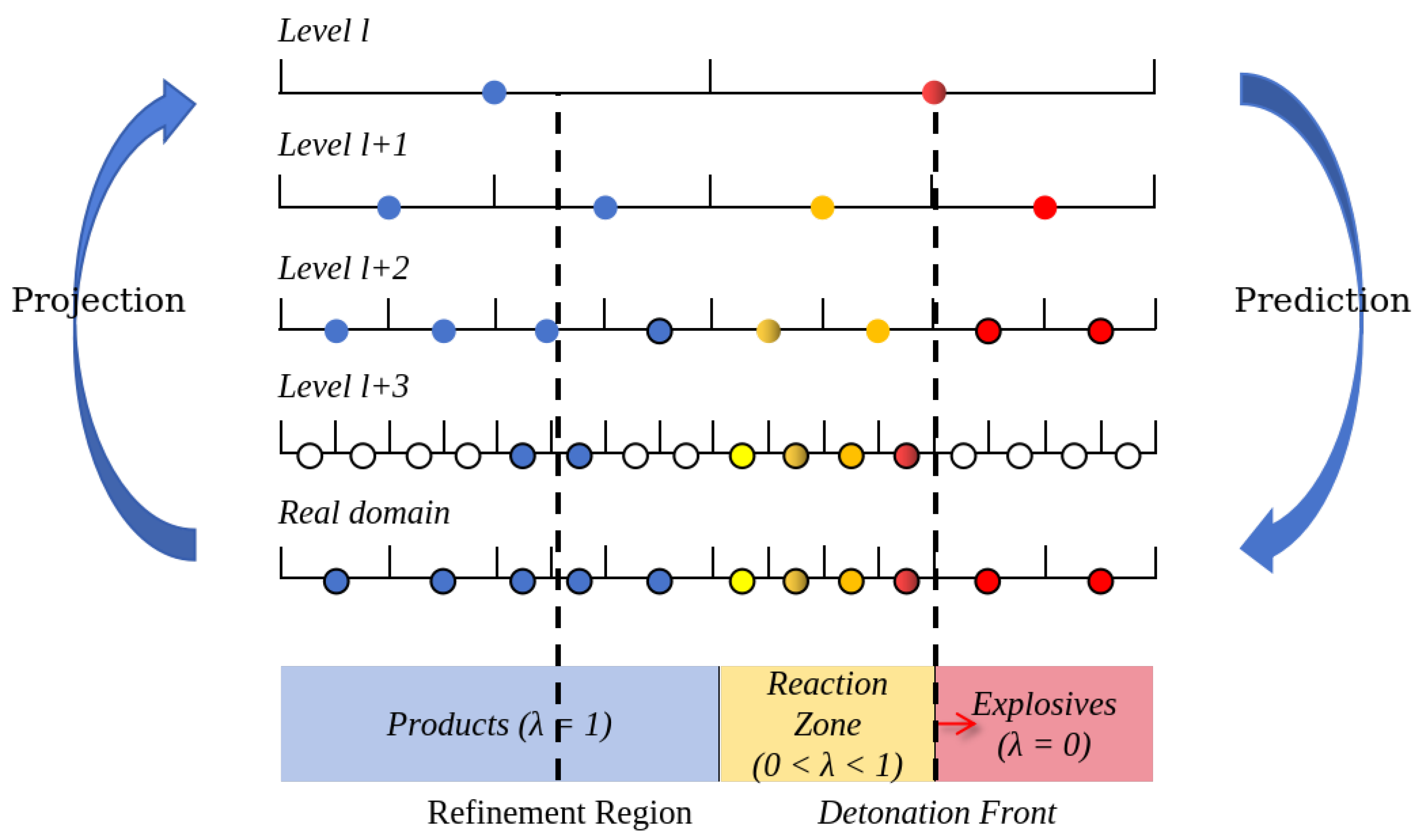
Schematic of the adaptive multi-resolution method for condensed-phase detonation. The arrow indicates the propagation direction of the detonation wave, which moves to the right, with the reaction zone behind it. Circles with black outlines denote leaf nodes, while circles without black outlines denote nodes containing child nodes; filled circles denote valid nodes, and open circles denote empty nodes. The colors distinguish the three regions of the computational domain: product zone (blue, ), reaction zone (orange, ), and unreacted explosive zone (red, ).
Figure 1.
Schematic of the adaptive multi-resolution method for condensed-phase detonation. The arrow indicates the propagation direction of the detonation wave, which moves to the right, with the reaction zone behind it. Circles with black outlines denote leaf nodes, while circles without black outlines denote nodes containing child nodes; filled circles denote valid nodes, and open circles denote empty nodes. The colors distinguish the three regions of the computational domain: product zone (blue, ), reaction zone (orange, ), and unreacted explosive zone (red, ).
Figure 2.
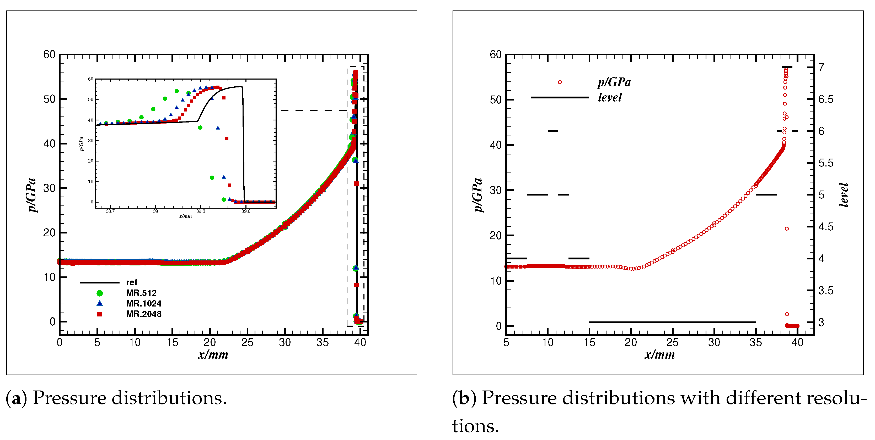
This figure contains two subfigures. (a) Pressure profile comparison: blue circles, green triangles, and red squares denote numerical results with maximum resolutions of 512, 1024, and 2048, respectively; the black solid line denotes the reference solution. (b) Pressure distributions and adaptive multi-resolution refinement-level distribution at a maximum computational level of 7.
Figure 2.
This figure contains two subfigures. (a) Pressure profile comparison: blue circles, green triangles, and red squares denote numerical results with maximum resolutions of 512, 1024, and 2048, respectively; the black solid line denotes the reference solution. (b) Pressure distributions and adaptive multi-resolution refinement-level distribution at a maximum computational level of 7.
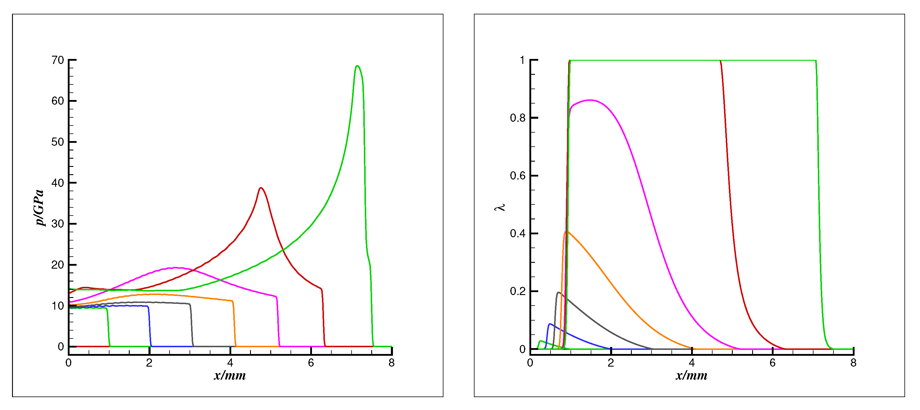
Figure 3.
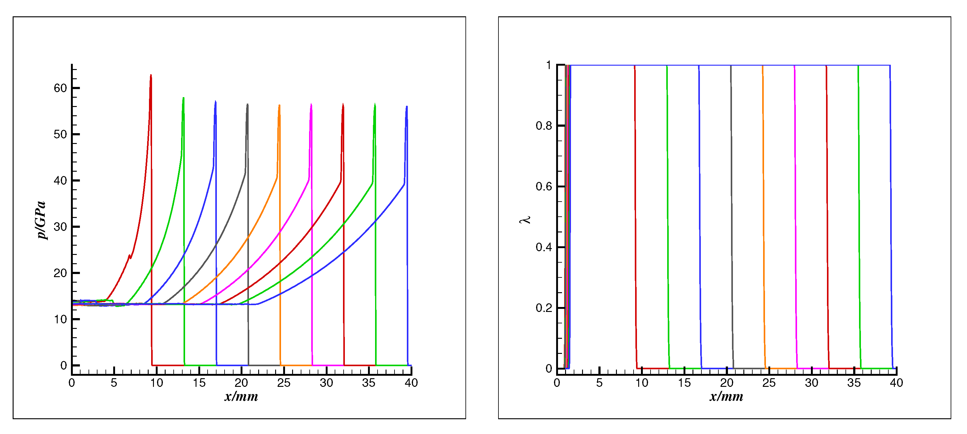
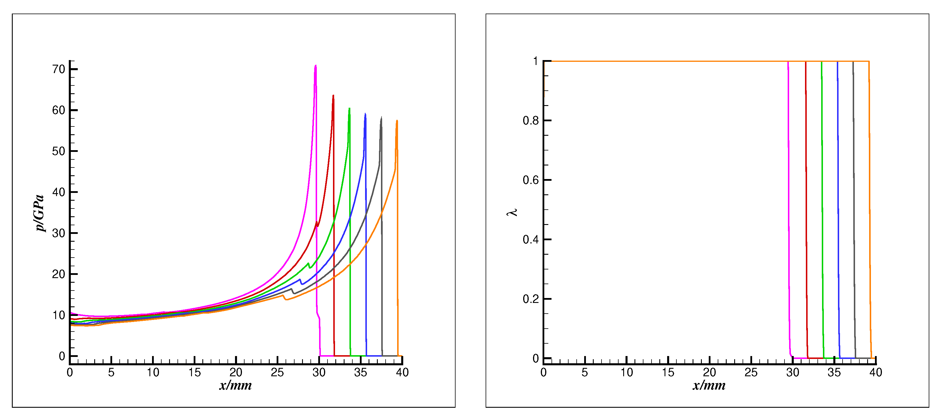
Stage 1: pressure p (left) and reaction progress variable (right) distributions at to with a time interval of . Different colored curves denote successive temporal snapshots within this time interval.
Figure 3.
Stage 1: pressure p (left) and reaction progress variable (right) distributions at to with a time interval of . Different colored curves denote successive temporal snapshots within this time interval.
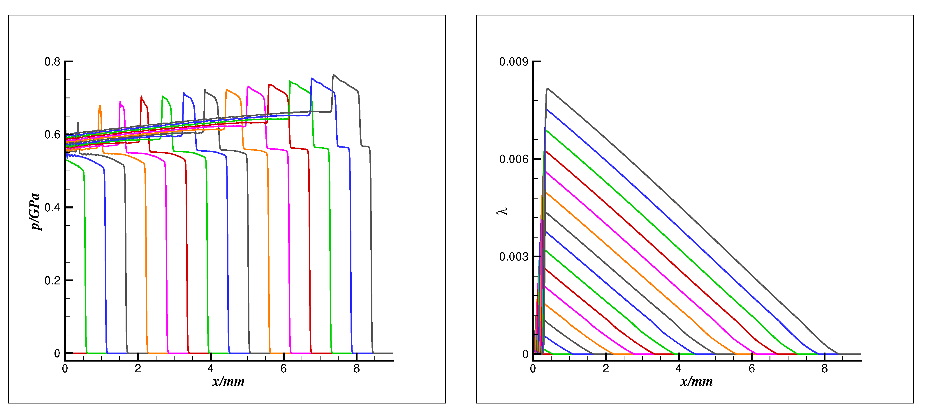
Figure 4.
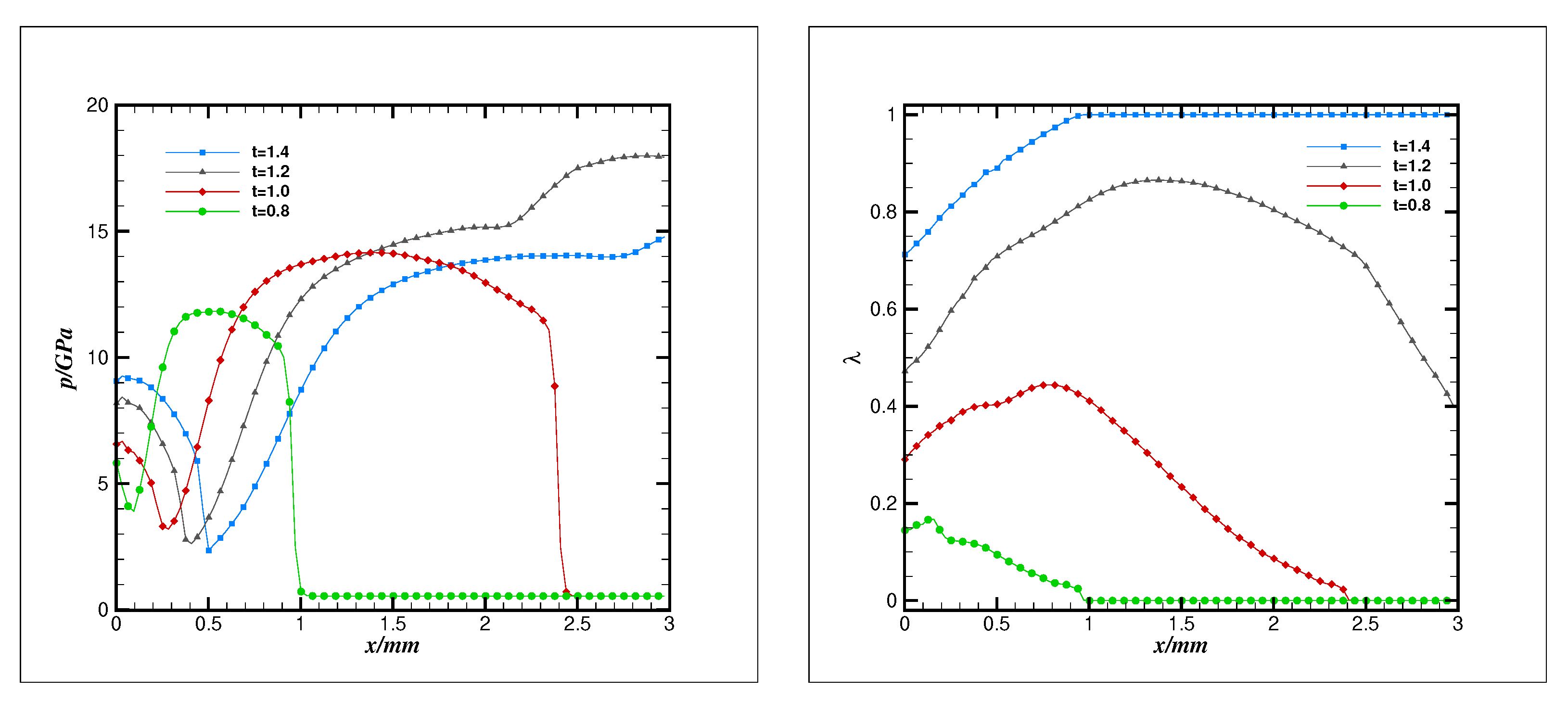
Stage 2: pressure p (left) and reaction progress variable (right) distributions at to with a time interval of . Different colored curves denote successive temporal snapshots within this time interval.
Figure 4.
Stage 2: pressure p (left) and reaction progress variable (right) distributions at to with a time interval of . Different colored curves denote successive temporal snapshots within this time interval.
Figure 5.
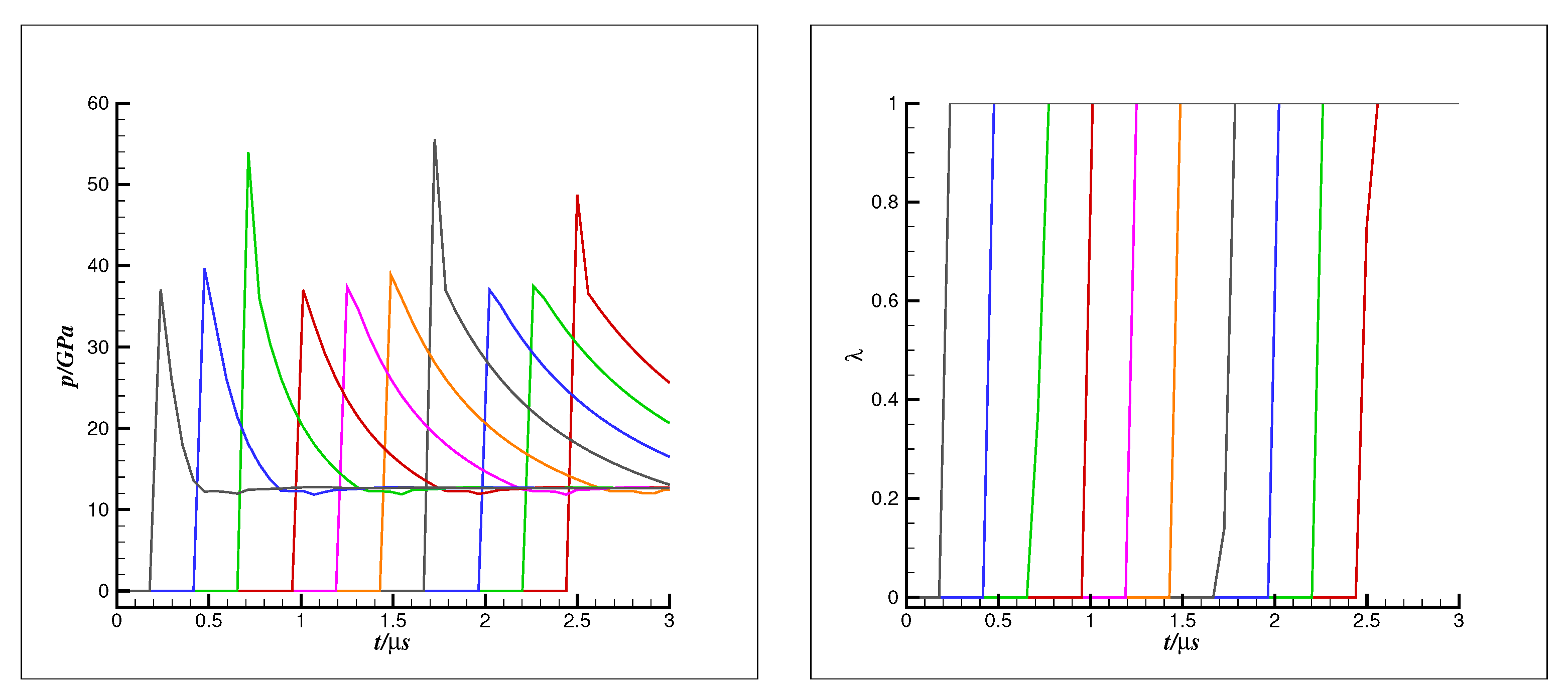
Tracer point histories of pressure p (left) and reaction progress variable (right) for the 1D strong shock initiation case. Different colored curves denote histories recorded at different tracer-point locations along the propagation direction.
Figure 5.
Tracer point histories of pressure p (left) and reaction progress variable (right) for the 1D strong shock initiation case. Different colored curves denote histories recorded at different tracer-point locations along the propagation direction.
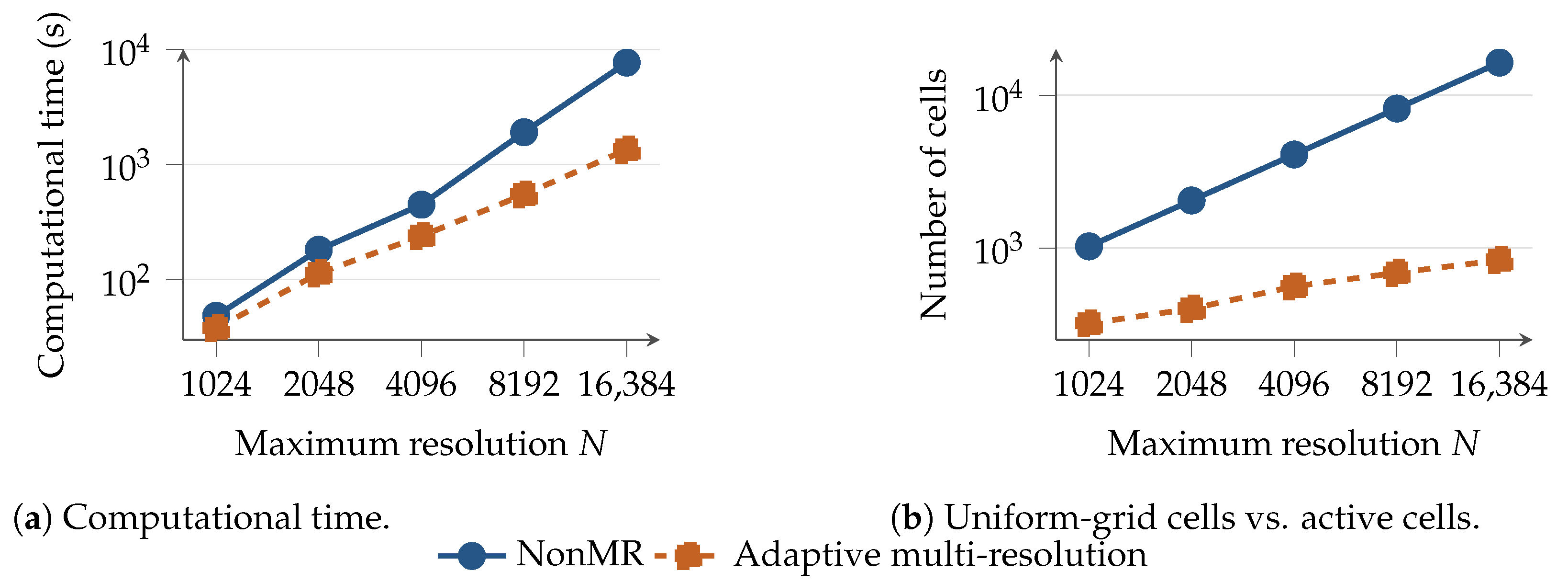
Figure 6.
Direct comparison between the uniform-grid (NonMR) and the adaptive multi-resolution computations for the 1D strong-shock initiation benchmark. Both vertical axes are logarithmic.
Figure 6.
Direct comparison between the uniform-grid (NonMR) and the adaptive multi-resolution computations for the 1D strong-shock initiation benchmark. Both vertical axes are logarithmic.
Figure 7.
Stage 1: pressure p (left) and reaction progress variable (right) distributions at to . Different colored curves denote successive temporal snapshots within this time interval.
Figure 7.
Stage 1: pressure p (left) and reaction progress variable (right) distributions at to . Different colored curves denote successive temporal snapshots within this time interval.
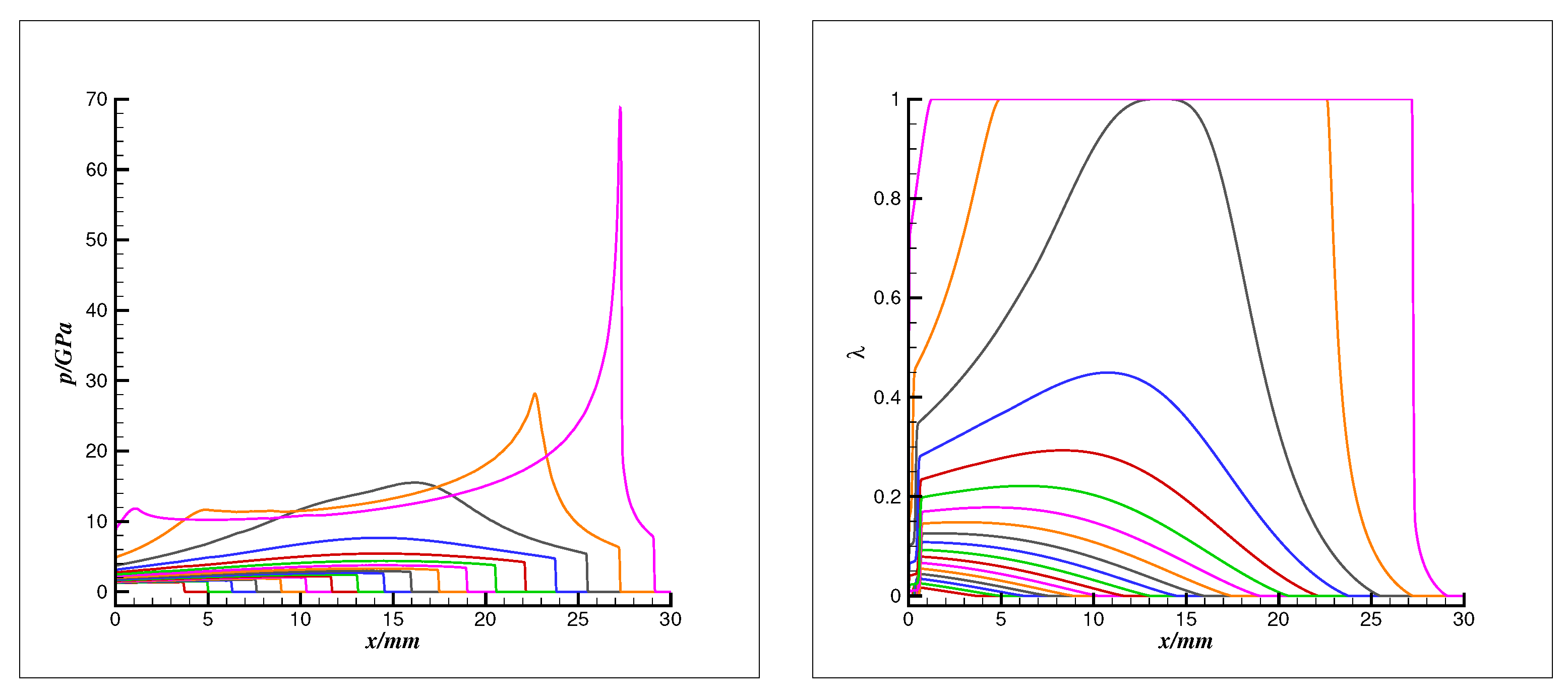
Figure 8.
Stage 2: pressure p (left) and reaction progress variable (right) distributions at to . Different colored curves denote successive temporal snapshots within this time interval.
Figure 8.
Stage 2: pressure p (left) and reaction progress variable (right) distributions at to . Different colored curves denote successive temporal snapshots within this time interval.
Figure 9.
Stage 3: pressure p (left) and reaction progress variable (right) distributions at to . Different colored curves denote successive temporal snapshots within this time interval.
Figure 9.
Stage 3: pressure p (left) and reaction progress variable (right) distributions at to . Different colored curves denote successive temporal snapshots within this time interval.
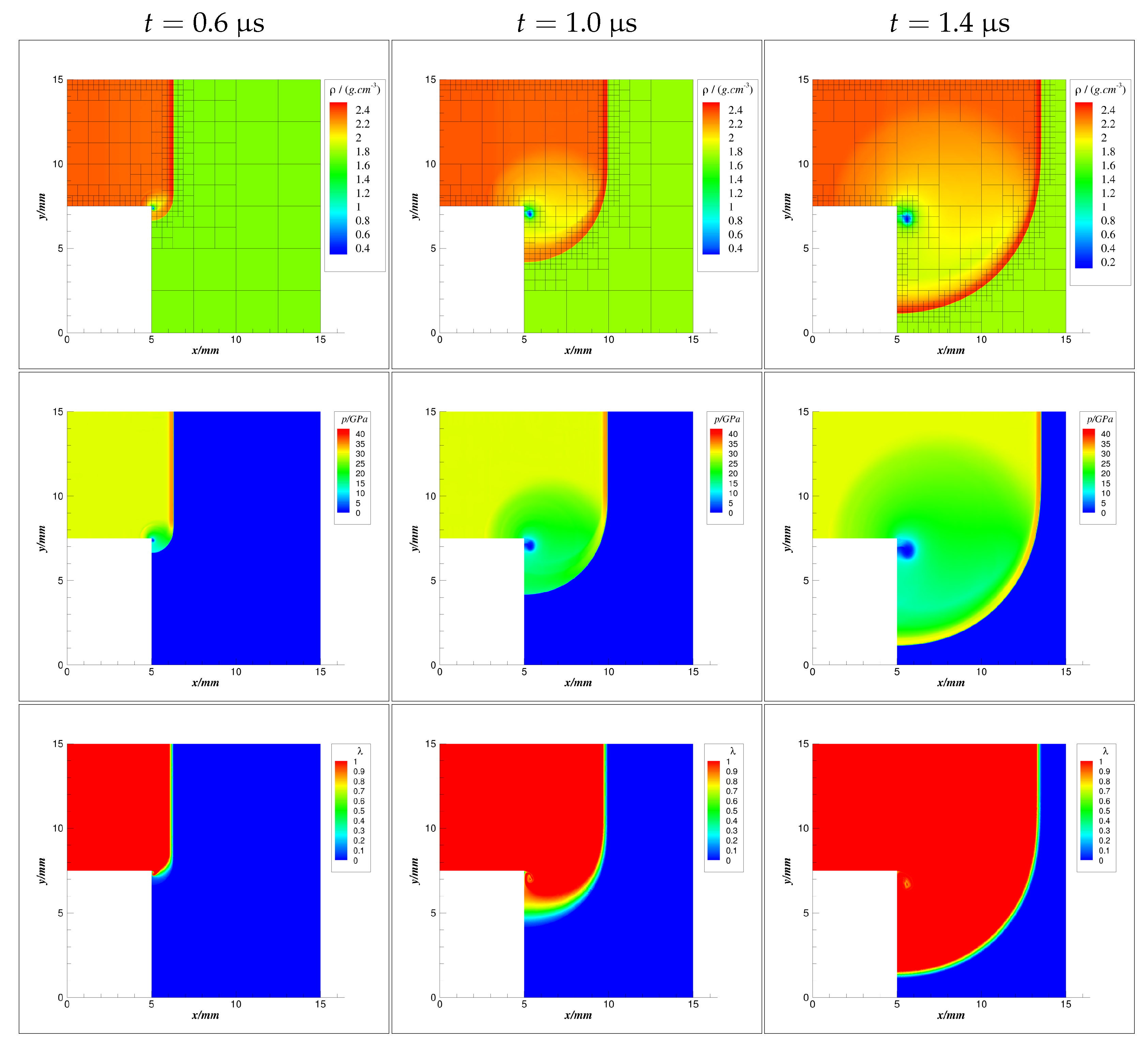
Figure 10.
Density (with multi-resolution block structure), pressure, and reaction progress variable distributions from top to bottom at , , and from left to right, respectively, for the corner diffraction problem.
Figure 10.
Density (with multi-resolution block structure), pressure, and reaction progress variable distributions from top to bottom at , , and from left to right, respectively, for the corner diffraction problem.
Figure 11.
Pressure p (left) and reaction progress variable (right) distributions along the inner wall at for to .
Figure 11.
Pressure p (left) and reaction progress variable (right) distributions along the inner wall at for to .
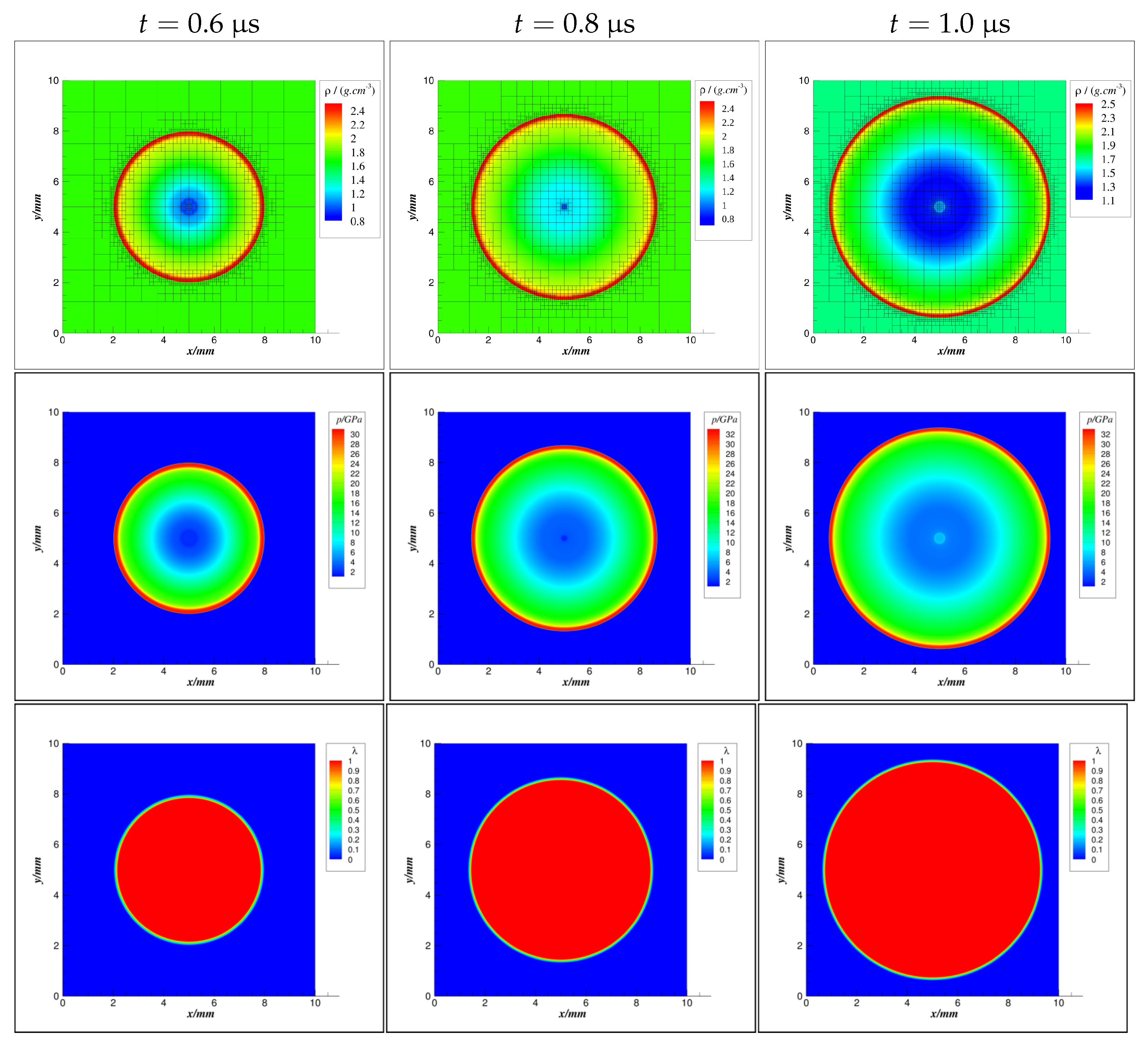
Figure 12.
Density (with multi-resolution block structure), pressure, and reaction progress variable distributions from top to bottom at , , and from left to right, respectively.
Figure 12.
Density (with multi-resolution block structure), pressure, and reaction progress variable distributions from top to bottom at , , and from left to right, respectively.
Figure 13.
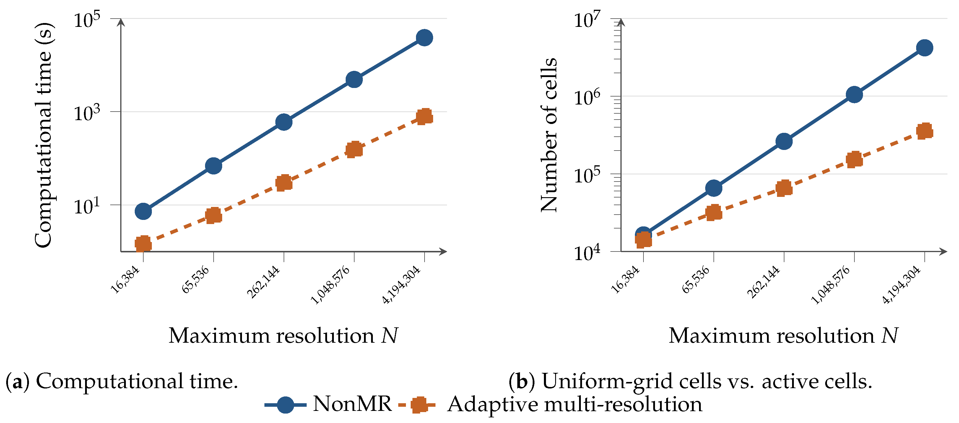
Direct comparison between the uniform-grid (NonMR) and adaptive multi-resolution computations for the 2D center-initiation benchmark. The x-axis tick labels are rotated and comma-separated to improve readability. Both vertical axes are logarithmic.
Figure 13.
Direct comparison between the uniform-grid (NonMR) and adaptive multi-resolution computations for the 2D center-initiation benchmark. The x-axis tick labels are rotated and comma-separated to improve readability. Both vertical axes are logarithmic.
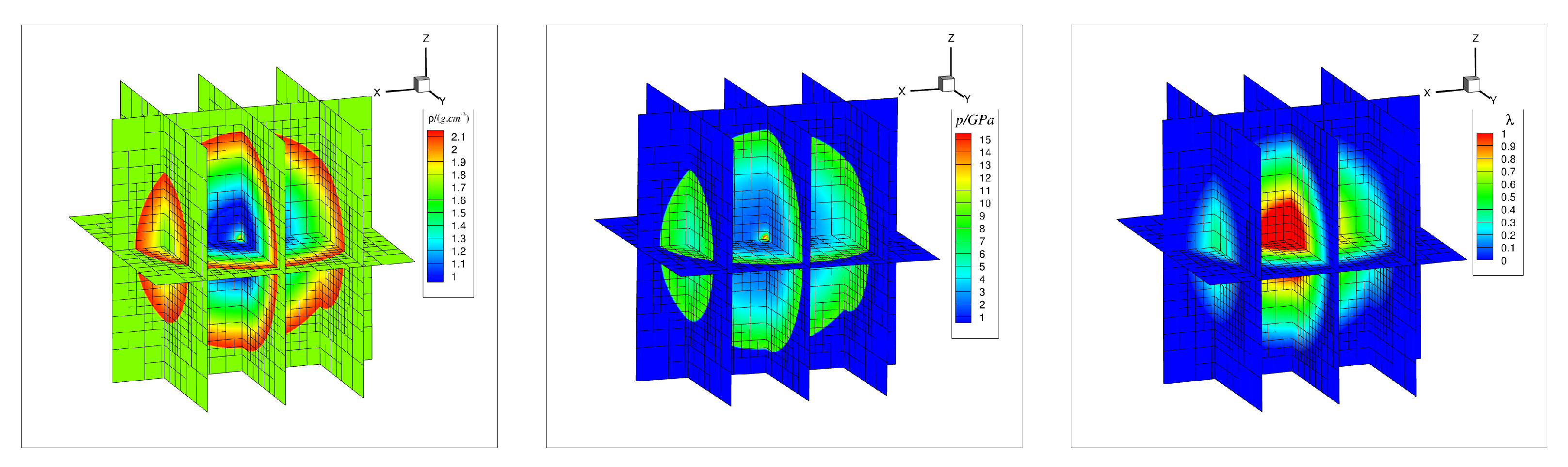
Figure 14.
Three-dimensional center-initiation results at . From left to right: density , pressure p, and reaction progress variable shown on the three orthogonal mid-plane slices (, , and ), with the multi-resolution block structure overlaid in each panel. The adaptive multi-resolution method concentrates refinement near the expanding spherical detonation front.
Figure 14.
Three-dimensional center-initiation results at . From left to right: density , pressure p, and reaction progress variable shown on the three orthogonal mid-plane slices (, , and ), with the multi-resolution block structure overlaid in each panel. The adaptive multi-resolution method concentrates refinement near the expanding spherical detonation front.
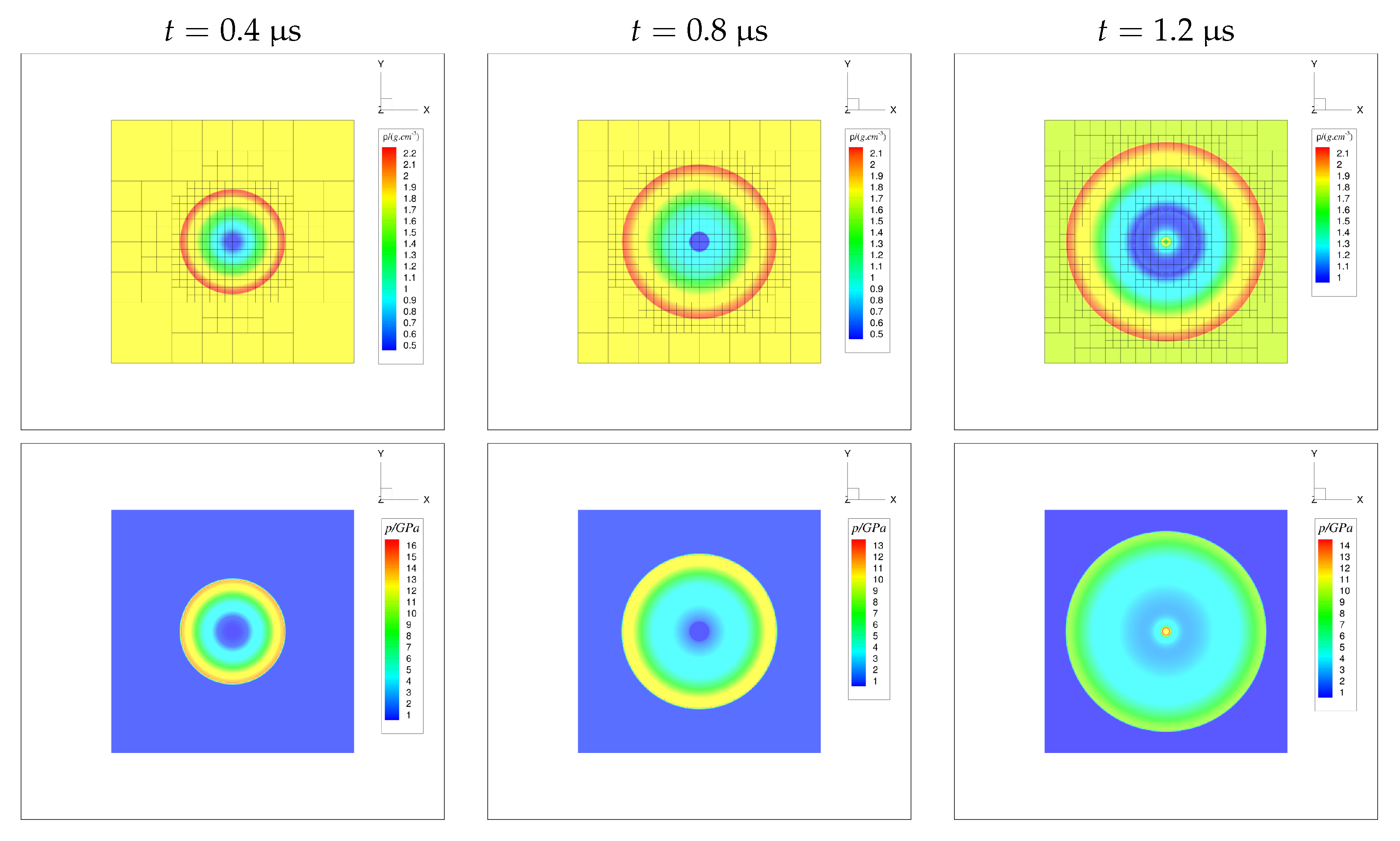
Figure 15.
slice contour maps for the three-dimensional center-initiation case. Top row: density ; bottom row: pressure p. Columns correspond to , , and (left to right). The overlapping “Z” label does not affect the scientific interpretation of the contour fields.
Figure 15.
slice contour maps for the three-dimensional center-initiation case. Top row: density ; bottom row: pressure p. Columns correspond to , , and (left to right). The overlapping “Z” label does not affect the scientific interpretation of the contour fields.
Figure 16.
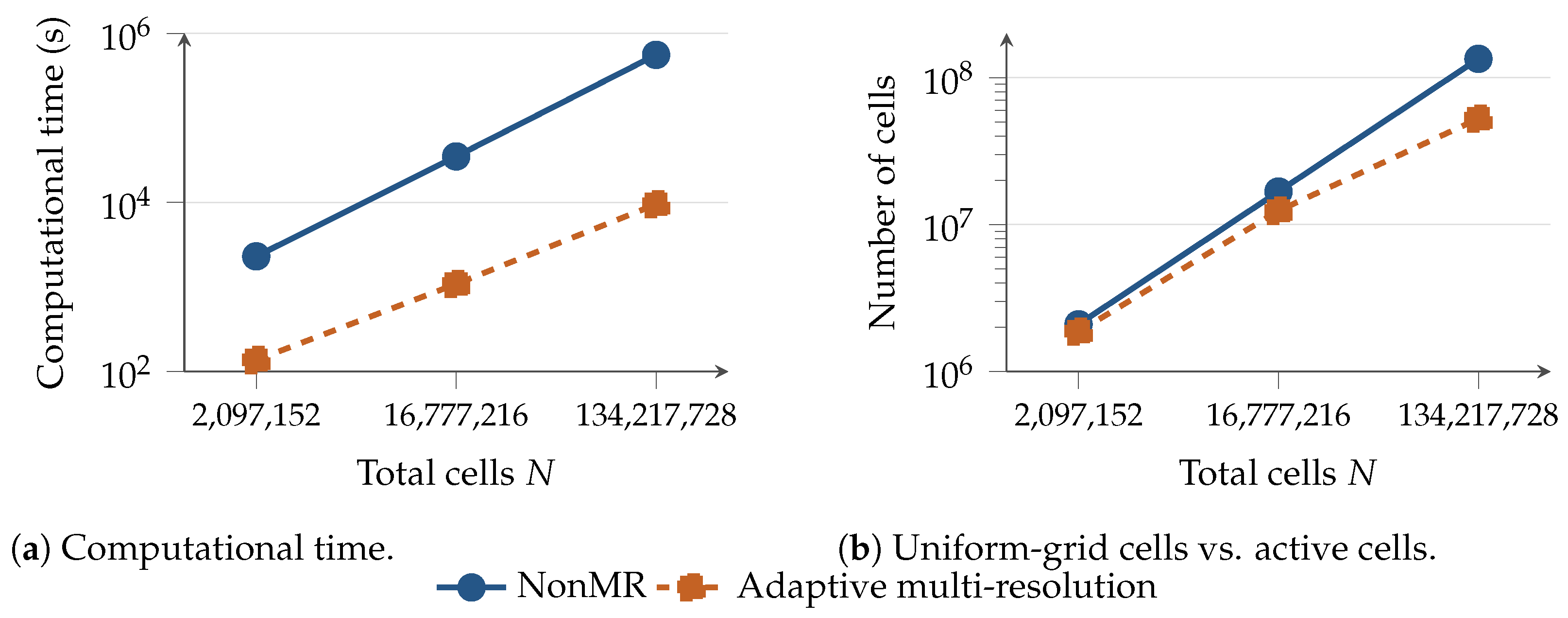
Direct comparison between the uniform-grid (NonMR) and adaptive multi-resolution computations for the 3D center-initiation benchmark. Both vertical axes are logarithmic.
Figure 16.
Direct comparison between the uniform-grid (NonMR) and adaptive multi-resolution computations for the 3D center-initiation benchmark. Both vertical axes are logarithmic.
Table 1.
EOS data for the explosive PBX-9404.
Table 1.
EOS data for the explosive PBX-9404.
| Parameter | Unreacted | Products |
|---|
| A () | 69.69 | 8.524 |
| B () | −1.727 | 0.1802 |
| () | | |
| 7.8 | 4.6 |
| 3.9 | 1.3 |
| 0.8578 | 0.38 |
| () | 1.842 | 1.842 |
Table 2.
EOS data for the explosive Comp-B.
Table 2.
EOS data for the explosive Comp-B.
| Parameter | Unreacted | Products |
|---|
| A () | 778.1 | 5.242 |
| B () | −0.05031 | 0.07678 |
| () | | |
| 11.3 | 4.2 |
| 1.13 | 1.1 |
| 0.8938 | 0.5 |
| () | 1.717 | 1.717 |
Table 3.
Lee–Tarver reaction rate parameters for PBX-9404.
Table 3.
Lee–Tarver reaction rate parameters for PBX-9404.
| Parameter | Value | Parameter | Value |
|---|
| I | | b | 0.667 |
| a | 0.0 | x | 20.0 |
| 3.1 | c | 0.667 |
| d | 0.111 | y | 1.0 |
| 400 | e | 0.333 |
| g | 1.0 | z | 2.0 |
Table 4.
Lee–Tarver reaction rate parameters for Comp-B.
Table 4.
Lee–Tarver reaction rate parameters for Comp-B.
| Parameter | Value | Parameter | Value |
|---|
| I | | b | 0.667 |
| a | 0.0367 | x | 7.0 |
| 140 | c | 0.667 |
| d | 0.333 | y | 2.0 |
| 1000 | e | 0.222 |
| g | 1.0 | z | 3.0 |
Table 5.
Comparison of computational cost and data storage between the uniform-grid and the adaptive multi-resolution method.
Table 5.
Comparison of computational cost and data storage between the uniform-grid and the adaptive multi-resolution method.
| N | 1024 | 2048 | 4096 | 8192 | 16,384 |
|---|
| (s) | 48.55 | 181.89 | 448.01 | 1911.00 | 7678.12 |
| (s) | 37.82 | 113.47 | 239.47 | 548.56 | 1346.82 |
| 22.10% | 37.62% | 46.55% | 71.29% | 82.46% |
| 1024 | 2048 | 4096 | 8192 | 16384 |
| 320 | 400 | 560 | 688 | 832 |
| 68.75% | 80.47% | 86.33% | 91.60% | 94.92% |
Table 6.
Compression metrics for the 2D center-initiation case at different uniform-grid resolutions.
Table 6.
Compression metrics for the 2D center-initiation case at different uniform-grid resolutions.
| N | 16,384 | 65,536 | 262,144 | 1,048,576 | 4,194,304 |
|---|
| (s) | 7.30 | 68.98 | 599.84 | 4906.91 | 38,754.3 |
| (s) | 1.47 | 5.97 | 29.76 | 154.64 | 789.41 |
| 79.86% | 91.35% | 95.04% | 96.85% | 97.96% |
| 16,384 | 65,536 | 262,144 | 1,048,576 | 4,194,304 |
| 14,080 | 31,744 | 65,536 | 153,088 | 355,840 |
| 14.06% | 51.56% | 75.00% | 85.40% | 91.52% |
Table 7.
Comparison of computational cost and data storage between the uniform-grid and the adaptive multi-resolution method for the 3D center-initiation case.
Table 7.
Comparison of computational cost and data storage between the uniform-grid and the adaptive multi-resolution method for the 3D center-initiation case.
| N | 2,097,152 | 16,777,216 | 134,217,728 |
|---|
| (s) | 2305.98 | 35,059.40 | 557,444.46 |
| (s) | 136.90 | 1085.52 | 9516.36 |
| 94.06% | 96.90% | 98.29% |
| 2,097,152 | 16,777,216 | 134,217,728 |
| 1,867,776 | 12,419,072 | 52,559,872 |
| 10.94% | 25.98% | 60.84% |