Fracturing Sweet Spot Evaluation and Prediction in Tight Sandstone Gas Reservoirs Using a GRA–LightGBM Hybrid Model

Abstract

The development of tight sandstone gas reservoirs in the Ordos Basin is increasingly challenged by complex geological conditions and declining resource quality. Accurate identification of productivity-controlling factors and reliable prediction of fracturing sweet spots are therefore essential for improving reservoir development efficiency. In this study, geological, engineering, and production data from 56 wells in the target area were collected and preprocessed using forward and reverse normalization. Grey Relational Analysis was first used to identify the dominant factors controlling absolute open flow, and the selected variables were then incorporated into Light Gradient Boosting Machine to establish an integrated GRA-LightGBM prediction framework. The results indicate that permeability, average total hydrocarbon content, porosity, brittleness index, fracture toughness, and clay content are the primary productivity-controlling factors in the study area. The proposed GRA-LightGBM model achieved an R² value of 0.9233, indicating strong agreement between predicted and measured AOF values. Comparative experiments with traditional machine learning models and tree-based ensemble models further demonstrated that GRA-LightGBM provides more accurate and stable predictions, with smaller residual fluctuations and better overall performance. Based on the prediction results, the spatial distribution of fracturing sweet spots was visualized using the Petrel platform. This study provides an effective data-driven workflow for dominant factor identification, AOF prediction, and sweet spot delineation, offering technical support for the optimization of hydraulic fracturing and well deployment in tight sandstone gas reservoirs.

1. Introduction

The Ordos Basin exhibits favorable natural gas accumulation conditions and hosts abundant natural gas resources. The Linxing area—situated on the Jinxi Fold Belt along the basin’s eastern margin—is strongly affected by tectonic uplift, leading to pronounced geological heterogeneity, suboptimal reservoir quality, and substantial development challenges. Consequently, stimulation effectiveness remains limited. Currently, hydraulic fracturing serves as the principal development technique for tight gas reservoirs in this region; thus, accurate identification and characterization of fracturing “sweet spots” are critical for optimizing well placement, target horizon selection, and perforation interval design—factors that ultimately govern single-well productivity and overall field development performance [1]. Accordingly, there is an urgent need to develop an intelligent sweet spot prediction methodology that standardizes data formats, integrates multi-source geological and engineering datasets, and comprehensively accounts for the complex interplay of geological and operational influencing factors.

Fracturing sweet spots can be broadly classified into geological and engineering sweet spots. Geological sweet spots denote zones characterized by hydrocarbon enrichment and constitute the fundamental geological foundation for the efficient development of unconventional oil and gas resources. Engineering sweet spots, in contrast, refer to reservoir intervals that exhibit favorable geomechanical and petrophysical properties—such as high brittleness and low stress anisotropy—thereby facilitating effective hydraulic fracturing and the creation of complex, interconnected fracture networks [2,3,4,5]. Conventional models—whether purely geological or engineering-based—often fall short in fully capturing the multifaceted characteristics of fracturing sweet spots, particularly due to the intricate, nonlinear interdependencies among reservoir parameters. To robustly identify the key productivity-controlling factors and achieve accurate, quantitative prediction of fracturing sweet spots, extensive research efforts have been undertaken both domestically and internationally. For instance, A. Ouenes integrated neural networks with fuzzy logic to jointly analyze 13 geological parameters; the resulting trained model enabled reliable prediction of Estimated Ultimate Recovery (EUR) and systematic identification of dominant controls on fracture propagation in tight gas reservoirs [6]. Bakay et al. integrated geostatistical modeling with machine learning to forecast production performance in shale reservoirs, using the Eagle Ford shale as a case study. Their work demonstrated that combining geological modeling and data-driven learning methods can improve reservoir characterization and provide useful support for production prediction and development decision-making in unconventional reservoirs [7]. Liu Fan introduced a novel sweet spot prediction methodology tailored for complex shale reservoirs, integrating an enhanced multi-threshold BIRCH clustering algorithm, a phase-controlled porosity prediction model, and the Analytic Hierarchy Process (AHP) to improve spatial resolution and predictive accuracy [8]. Ahmed Algarhy developed a Sweet Spot Quality Index (SSQI) model by integrating the Reservoir Quality Index (RQI), Completion Quality Index (CQI), Conventional Productivity Index (CPI), and Operational Index (OI) using a random forest algorithm. A sensitivity analysis was conducted to quantify the relative influence of multiple input parameters on sweet spot quality. The model was further refined through Monte Carlo simulations, which incorporated reservoir geological, completion, and economic parameters—thereby enabling robust prediction of shale production performance along with comprehensive uncertainty quantification [9,10]. Han Kemei proposed a Particle Swarm Optimization–Support Vector Machine (PSO-SVM) model for integrated geological–engineering sweet spot prediction [11]. Yang Dongxue constructed an XGBoost-based machine learning model to predict the spatial distribution of sweet spots by jointly leveraging geological features and seismic attributes [12]. Yuxuan Deng introduced a data-driven, automated workflow for building an integrated sweet spot evaluation model. This approach quantifies key fracturability and flowability parameters and combines them with independent weight coefficient methods and a deep clustering autoencoder algorithm [13]. JIANG Fujie established a shale oil enrichment control factor model grounded in core observations, experimental analyses, and integrated geological studies, systematically evaluating the influences of organic richness, storage capacity, hydrocarbon migration efficiency, and lithofacies heterogeneity on enrichment patterns [14]. LIU Gaofeng employed data normalization and fuzzy proximity calculations to integrate geological and production data, thereby developing a fuzzy pattern recognition (FPR) model for sweet spot grading that eliminates subjective weighting [15]. Xiao Xiao et al. developed a shale gas sweet spot parameter prediction model based on the LightGBM regression algorithm [16].

Existing fracturing sweet spot prediction methods still have several critical limitations. First, conventional data preprocessing methods commonly apply uniform normalization to all variables, which may weaken the directional physical meanings of different geological and engineering parameters. In fact, some parameters are positively correlated with productivity, whereas others may exert negative or nonlinear effects. Ignoring these differences may reduce the physical interpretability of the input feature system. Second, many previous studies have mainly focused on improving prediction accuracy, while the incorporation of geological and engineering mechanisms controlling production behavior into feature construction remains insufficient. Third, although hybrid models combining feature selection methods and machine learning algorithms have been reported, most of them use feature selection only as a general dimensionality-reduction step. The selected variables are often not explicitly linked to reservoir productivity mechanisms or to the directional effects of geological and engineering parameters. Fourth, for tight sandstone gas reservoirs with limited well samples and strong heterogeneity, the robustness and interpretability of machine learning-based sweet spot prediction still require further improvement. Based on these considerations, this study proposes a GRA-LightGBM framework for fracturing sweet spot prediction in the Linxing tight sandstone gas reservoir. The proposed framework first incorporates geological and engineering understanding into the selection of candidate indicators, then applies GRA to determine the dominant productivity-controlling factors, and finally uses LightGBM to establish the nonlinear mapping between the selected factors and reservoir productivity. Through this workflow, the model provides an interpretable and data-driven approach for identifying fracturing sweet spots under complex geological–engineering coupling conditions.

Specifically, geological, engineering, and production data from 56 wells in the eastern Linxing area of the Ordos Basin were systematically collected and processed. First, according to the theoretical and empirical relationships between each parameter and AOF, geological and engineering parameters were classified into positively and negatively influential variables and were processed using forward and reverse normalization, respectively. This strategy ensures dimensional consistency and comparability among variables while preserving the directional influence of different factors on production performance. Second, Grey Relational Analysis was used to quantify the grey relational degree between each candidate parameter and AOF. In this study, GRA is used not only as a statistical feature selection tool but also as a grey sensitivity analysis method to identify dominant productivity-controlling factors from a coupled geological–engineering perspective. Subsequently, the key factors selected by GRA were used as input variables for the LightGBM regression model to construct a compact and physically meaningful feature set, thereby reducing the interference of redundant information in model training and improving model interpretability. Finally, the LightGBM model was optimized using GridSearchCV and an early stopping strategy. Meanwhile, model performance was compared using different numbers of GRA-ranked features, including the top 3, 4, 5, 6, 8, and all 10 features, to further verify the rationality and robustness of the selected dominant-factor combination. The validation results demonstrate that the proposed GRA-LightGBM model can effectively capture the nonlinear relationships between geological–engineering factors and AOF, providing reliable theoretical support and technical guidance for fracturing sweet spot identification, well and formation selection, and hydraulic fracturing design optimization in the Linxing area.

2. Methodology and Principles

2.1. Traditional LightGBM Model

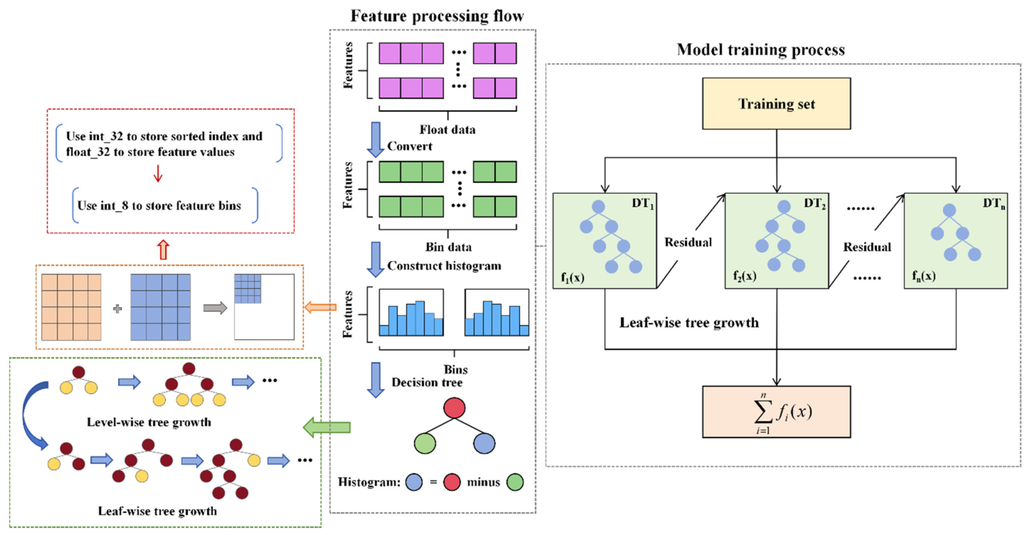
LightGBM is an efficient implementation of the Gradient Boosting Decision Tree (GBDT) algorithm, which iteratively constructs decision trees to fit the residuals of previous models and improve prediction performance [17,18]. Compared with conventional GBDT algorithms, LightGBM improves computational efficiency through histogram-based feature discretization and a leaf-wise tree growth strategy with depth constraints. The histogram algorithm reduces memory usage and training cost by transforming continuous features into discrete bins, while the leaf-wise strategy can achieve lower loss under the same number of splits. In addition, Gradient-based One-Side Sampling (GOSS) and Exclusive Feature Bundling (EFB) are used to reduce data redundancy and computational complexity, making LightGBM suitable for nonlinear prediction tasks involving multiple geological and engineering parameters [19,20,21,22] (see Figure 1).

2.2. Grey Relational Analysis (GRA)

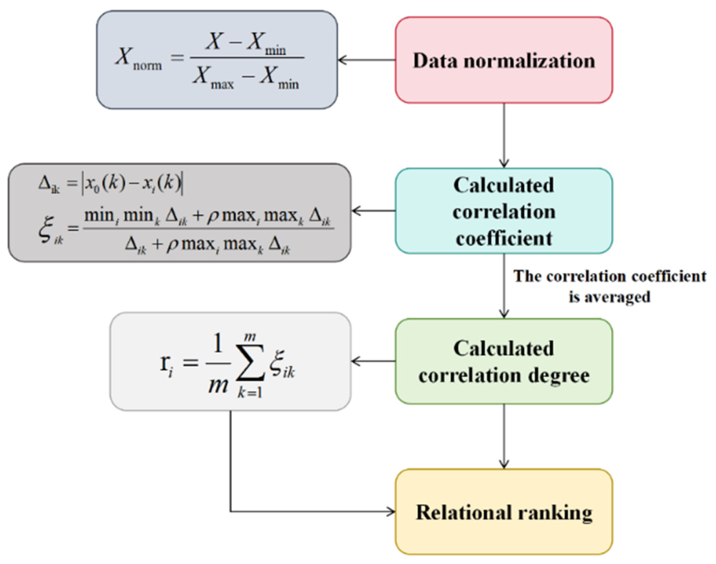
Grey Relational Analysis (GRA) is a method used to quantify the degree of association among factors within a system [23] (Figure 2). The fundamental principle of GRA is to assess the closeness of relationships based on the geometric similarity of sequence curves: the more similar the shapes of the curves, the stronger the correlation between the corresponding sequences; conversely, the less similar the curves, the weaker the correlation. This approach enables the evaluation of how strongly each factor influences the target variable. GRA is particularly well-suited for analyzing complex systems characterized by small sample sizes and incomplete information.

2.3. Construction of the GRA-LightGBM-Based Sweet Spot Prediction Model

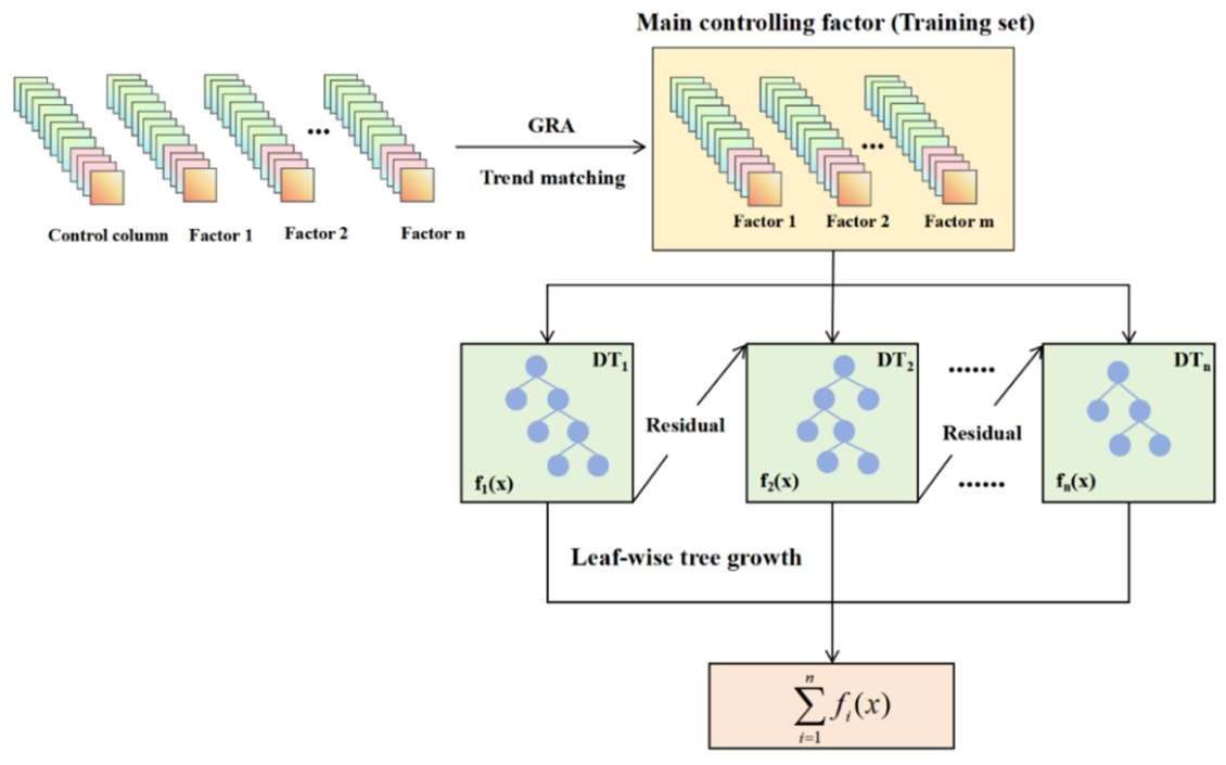
Despite the powerful capabilities and performance advantages of LightGBM, directly applying it for dominant factor selection and sweet spot prediction still presents several challenges. Feature selection in LightGBM models is typically conducted using techniques such as Recursive Feature Elimination or SHapley Additive exPlanations. Nevertheless, as these methods are inherently dependent on the training process, their results may be biased or unstable when applied to datasets with particular distributions or limited representativeness. LightGBM evaluates the contribution of each feature to the model by calculating metrics such as the number of times a feature is used to split tree nodes (based on gain, e.g., Gini gain) or the number of samples covered by those splits (frequency) [24]. However, these importance scores are obtained post-training and do not inherently reflect the intrinsic relationships among variables. Consequently, redundant features cannot be excluded prior to training, resulting in unnecessary computational overhead. While the Exclusive Feature Bundling (EFB) technique reduces computational complexity for high-dimensional data, irrelevant features can still increase split complexity, slow down training, and inflate memory usage. Furthermore, noisy features within datasets may lead to model overfitting—particularly in small-sample scenarios—where LightGBM may erroneously learn from noise rather than signal. To address these issues—namely, reducing computational cost, suppressing noise interference, ensuring accurate feature selection, and enabling applicability to small-sample, low-information settings—this study proposes a hybrid GRA-LightGBM model (Figure 3).

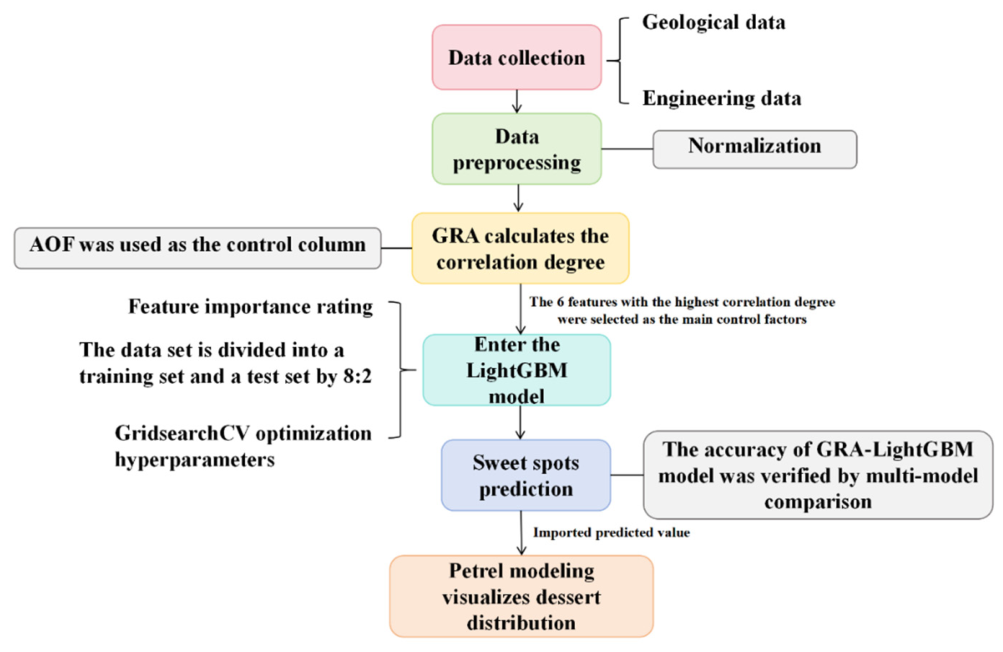
GRA is well-suited for complex system analysis with limited data and incomplete information. It evaluates variable importance based on the relative trend of data variation [23,25], independent of data scale and distribution. By identifying dominant factors from the perspective of intrinsic correlation, GRA complements the limitations of standalone LightGBM in feature selection. A relevance-driven feature selection mechanism filters redundant information and tailors the input space for the LightGBM model, allowing it to concentrate on high-impact features and thereby enhancing its efficiency in learning complex geological patterns. This allows the model to focus on high-contribution features, substantially improving its learning efficiency in complex geological settings. The dominant factors identified by GRA are further evaluated using LightGBM scoring, providing a “model-based” validation of their predictive value. This integrated modeling strategy, which leverages the strengths of both methods, aligns more closely with the practical demands of hydraulic fracturing sweet spot prediction (Figure 4).

3. Validation and Analysis

3.1. Univariate Analysis

The dataset used in this study was derived from 56 wells in the Linxing East study area, all of which have available experimental and logging data. Geological parameters were obtained from logging, seismic interpretation, and laboratory tests, including total hydrocarbon average THA, porosity POR, permeability PER, initial gas saturation IGS, and volume of shale VSH. Engineering parameters were calculated based on logging data, including Young’s modulus Ed, Poisson’s ratio Ud, brittleness index BI, fracture toughness FT, and unconfined compressive strength UCS [26]. For each evaluation parameter, the average value across the fracturing interval was used. The reference column is the absolute open flow AOF of each well in the Linxing East study area, which serves as the target variable for productivity prediction (see

Table 1. Partial original dataset.

	POR	PER	IGS	VSH	THA	Ed	Ud	BI	UCS	FT	AOF
Minimum	8.09	0.29	38.32	3.27	0.95	15,553.69	0.30	0.50	4.50	0.04	0.10
Maximum	16.41	5.39	60.90	15.40	71.10	22,780.82	0.33	0.51	8.78	0.35	34.70
Mean	11.63	1.36	53.35	7.98	15.63	20,118.88	0.31	0.51	6.72	0.19	2.28
Standard deviation	1.76	0.90	3.78	2.68	14.43	1727.77	0.01	0.01	0.94	0.08	5.12
Unit	%	mD	%	%	%	MPa	dimensionless	dimensionless	MPa	MPa·m0.5	104 m3
Data source	Well logging	Core test	Well logging	Well logging	Mud logging	Well logging	Well logging	Calculated	Calculated	Calculated	Well test

).

Given the dimensional disparities among different features, directly feeding them into the model could cause the model to overemphasize high-magnitude features while neglecting those with lower magnitudes. This imbalance may degrade model performance. Therefore, normalization of the raw dataset was performed prior to modeling. Before normalization, the evaluation parameters were classified into positive and negative parameters according to their geological and engineering implications for hydraulic fracturing sweet spot evaluation. A positive parameter indicates that a higher value is generally favorable for gas enrichment, reservoir quality, or fracture stimulation, whereas a negative parameter indicates that a lower value is generally more favorable for fracturing effectiveness or reservoir development.

Specifically, THA, POR, PER, IGS, Ed, and BI were treated as positive parameters. Higher THA and IGS generally indicate better gas-bearing properties; higher POR and PER represent better storage capacity and seepage ability; higher Ed usually reflects greater rock stiffness; and higher BI indicates stronger brittleness, which is beneficial for fracture initiation and propagation. In contrast, VSH, Ud, FT, and UCS were treated as negative parameters. A higher VSH usually indicates stronger shale content and poorer reservoir quality; a higher Ud reflects stronger ductility and weaker brittleness; a higher FT indicates greater resistance to fracture propagation; and a higher UCS implies stronger rock strength and greater difficulty in fracture initiation (see

Table 2. Attributes and physical basis of evaluation parameters used for normalization.

Parameter	Full Name	Attribute	Physical Basis
THA	Total hydrocarbon average	Positive	Higher THA indicates stronger hydrocarbon/gas show and better gas-bearing potential.
POR	Porosity	Positive	Higher porosity indicates better reservoir storage capacity.
PER	Permeability	Positive	Higher permeability indicates better seepage capacity and gas deliverability.
IGS	Initial gas saturation	Positive	Higher gas saturation indicates better gas-bearing properties.
VSH	Volume of shale	Negative	Higher shale content may reduce reservoir quality and effective storage/seepage capacity.
Ed	Young’s modulus	Positive	Higher Young’s modulus generally reflects greater rock stiffness and is commonly associated with better fracability.
Ud	Poisson’s ratio	Negative	Higher Poisson’s ratio usually indicates stronger ductility and lower brittleness.
BI	Brittleness index	Positive	Higher brittleness favors fracture initiation and propagation during hydraulic fracturing.
FT	Fracture toughness	Negative	Higher fracture toughness means stronger resistance to fracture propagation.
UCS	Unconfined compressive strength	Negative	Higher UCS indicates stronger rock strength and greater difficulty in fracture initiation.

).

Accordingly, forward normalization was applied to positive parameters using Equation (1), whereas reverse normalization was applied to negative parameters using Equation (2).

$$X_{Forward}={\displaystyle \frac{x-\min }{\max -\min }}$$

(1)

$$X_{Reverse}={\displaystyle \frac{\max -x}{\max -\min }}$$

(2)

The target variable, Absolute Open Flow (AOF), was subjected to positive normalization to ensure consistency in scale with the feature variables. A subset of the processed sample data after normalization is shown in

Table 3. Partial sample data after normalization processing.

WN	POR	PER	IGS	VSH	THA	Ed	Ud	BI	UCS	FT	AOF
L-1	0.37	0.07	0.49	0.11	0.06	0.21	0.23	0.31	0.17	0.87	0.03
L-1-1D	0.27	0.07	0.76	0.83	0.12	0.86	0.87	0.54	0.66	0.37	0.01
L-2	0.13	0.08	0.74	0.59	0.19	0.75	0.77	0.29	0.55	0.38	0.05
L-3	0.25	0.06	0.12	0.45	0.08	0.73	0.77	0.29	0.57	0.38	0.14
L-3-4D	0.41	0.15	0.68	0.61	0.36	0.70	0.73	0.20	0.55	0.51	0.20

.

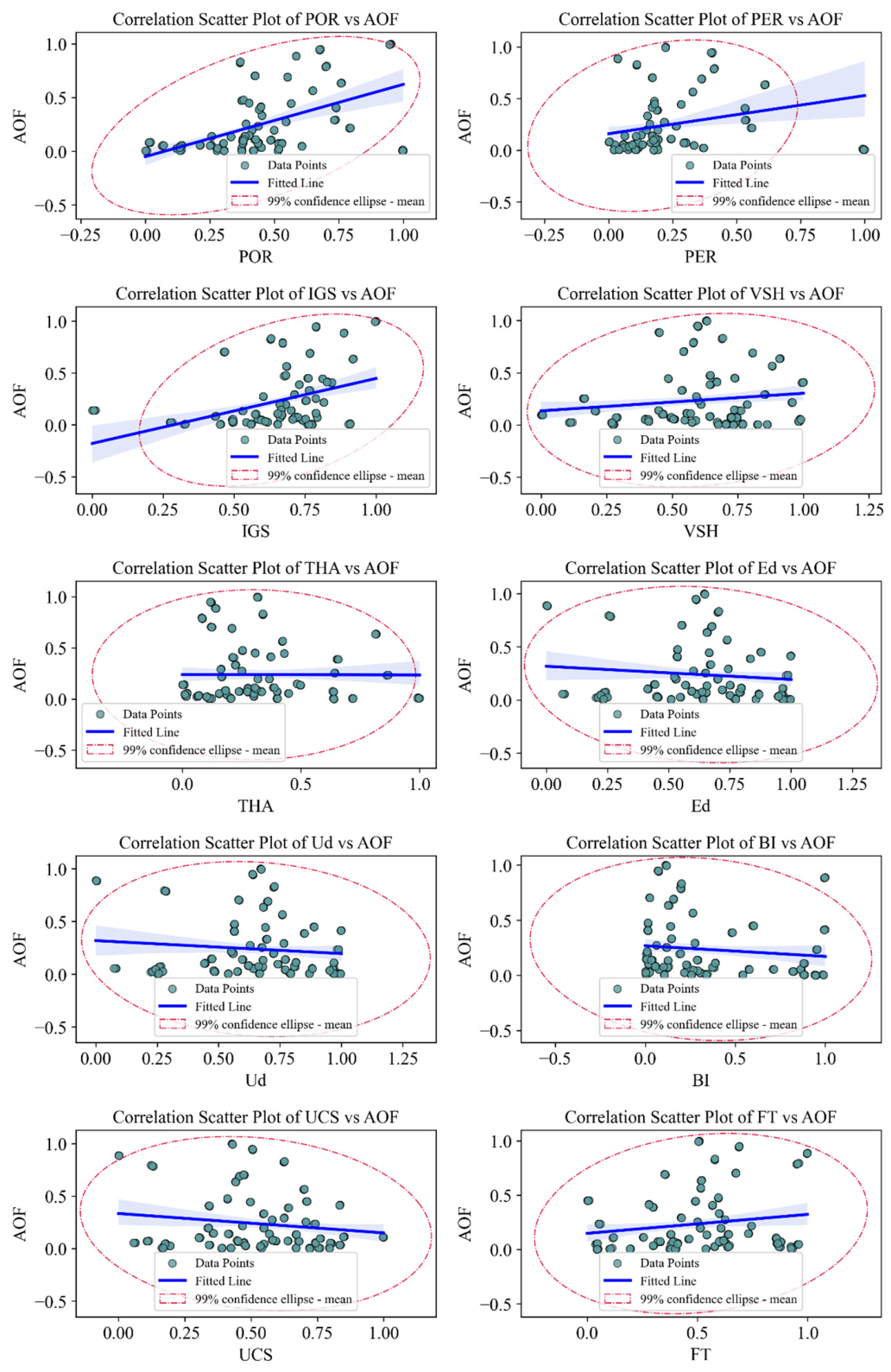
After data preprocessing, the relationships between each engineering and geological parameter and the AOF were analyzed (Figure 5).

As shown in Figure 5, variables such as porosity (POR), permeability (PER), and initial gas saturation (IGS) exhibit a certain degree of positive correlation with AOF, whereas Young’s modulus (Ed), Poisson’s ratio (Ud), and unconfined compressive strength (UCS) show a negative correlation, indicating that these factors may constrain fracturing productivity in sweet spot zones. In contrast, variables such as volume of Shale (VSH), brittleness index (BI), fracture toughness (FT), and total hydrocarbon average (THA) demonstrate near-zero regression slopes and wide confidence intervals, suggesting weak and statistically insignificant correlations. This analysis indicates that the correlation between any single factor and AOF is generally weak, making simple linear models insufficient to accurately characterize the mechanisms underlying sweet spot formation. Therefore, it is necessary to adopt a multi-variable interaction modeling approach to capture the complex interactions and nonlinear effects among variables, thereby improving the accuracy of sweet spot prediction in hydraulic fracturing.

3.2. Validation of the GRA-LightGBM Model

3.2.1. Selection of Dominant Factors

According to the principles of Grey Relational Analysis (GRA), a comparative sequence is constructed from the 10 evaluation parameters, and the Absolute Open Flow (AOF) is selected as the reference sequence to conduct sensitivity analysis between the AOF and each evaluation parameter. First, the normalized feature matrix is compared with the column vector of the target variable (AOF) to obtain the absolute difference matrix between each feature and the target variable. From this difference matrix, the global minimum and maximum values are identified. Using Equation (3), the grey relational coefficient for each feature is calculated. Then, the average of these coefficients across all samples for each feature is computed using Equation (4) to obtain the grey relational grade, which quantifies the degree of association between each feature and the AOF.

$${\xi }_i={\displaystyle \frac{{\Delta }_{\min }+\rho \cdot {\Delta }_{\max }}{{\Delta }_{i,j}+\rho \cdot {\Delta }_{\max }}}$$

(3)

$$r_i={\displaystyle \frac{1}{n}}{\displaystyle \sum _{j=1}^n{\xi }_{i,j}}$$

(4)

In this formula, ${\xi }_i$ denotes the grey relational coefficient of each evaluation factor; ${△}_{i,j}=\left|x_i-y_j\right|$ represents the absolute difference between the feature and the target; ${△}_{min}$ indicates the global minimum difference; ${△}_{max}$ indicates the global maximum difference; $\rho$ is the distinguishing coefficient, $0<\rho <1$ (commonly set to 0.5); $r_i$ denotes the relational grade of each feature; and $n$ represents the number of wells in the sample dataset.

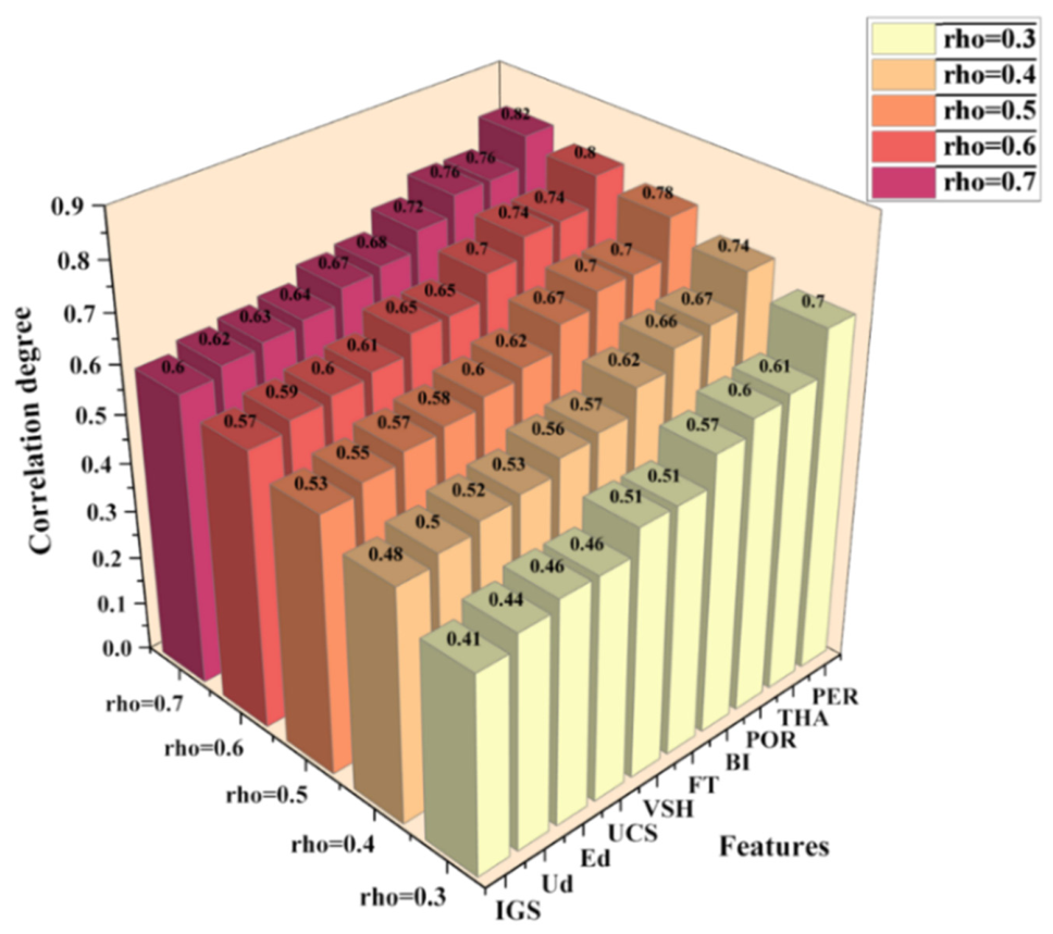
In GRA, the distinguishing coefficient $\rho$ is an important parameter that controls the resolution of the grey relational coefficient. A smaller ρ value enhances the contrast among different factors, whereas a larger ρ value weakens such differences. Therefore, to systematically evaluate the sensitivity of the GRA results to $\rho$, five commonly used values, namely 0.3, 0.4, 0.5, 0.6, and 0.7, were tested in this study. The grey relational grades between each influencing factor and AOF were recalculated under each $\rho$ setting, and the corresponding variations are shown in Figure 6. The results indicate that the absolute values of the grey relational grades vary with $\rho$. Specifically, smaller $\rho$ values lead to lower relational grades and greater differentiation among factors, whereas larger ρ values produce higher relational grades and reduced contrast. Nevertheless, the ranking of the dominant factors remains highly consistent under different $\rho$ settings. The six factors with the highest grey relational grades are consistently identified as permeability, average total hydrocarbon content, porosity, brittleness index, fracture toughness, and clay content. This indicates that the GRA-based identification of dominant productivity-controlling factors is not sensitive to the selection of $\rho$ and has good robustness. Considering that $\rho$ = 0.5 is widely used in GRA and provides a balanced discrimination between relational differences and numerical stability, this study ultimately adopted $\rho$ = 0.5 for the calculation of grey relational grades. The above sensitivity analysis further confirms the reliability and stability of the selected dominant factors.

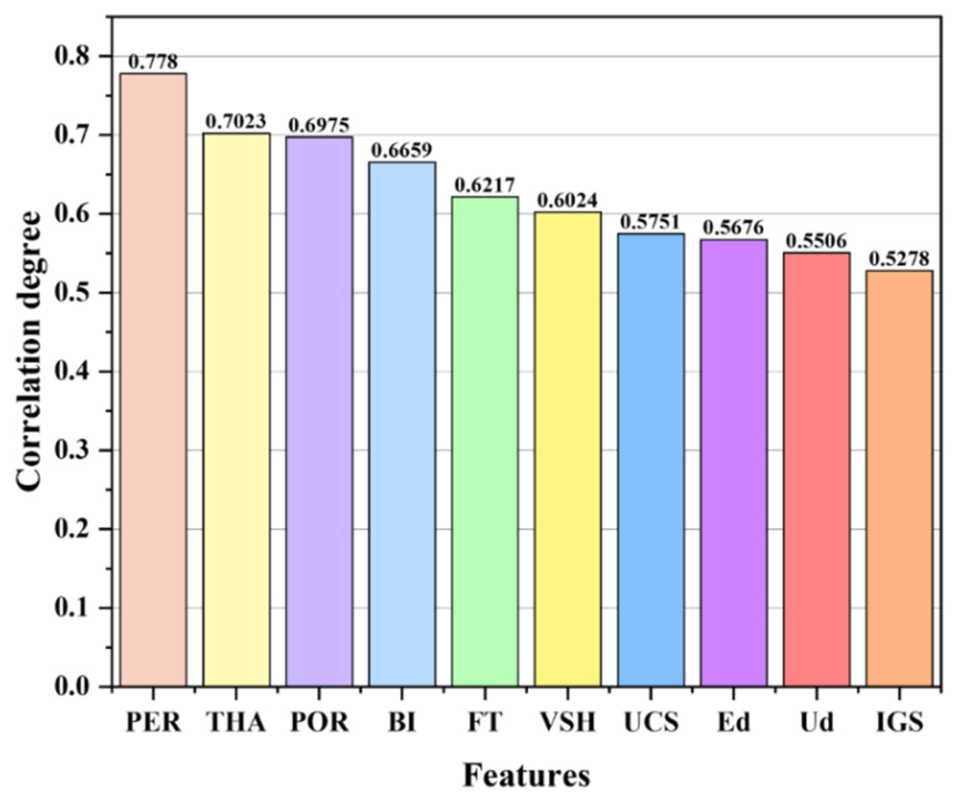
As shown in Figure 7, the grey relational grades between the input features and AOF are ranked in descending order as follows: PER (0.7780), THA (0.7023), POR (0.6975), BI (0.6659), FT (0.6217), VSH (0.6024), UCS (0.5751), Ed (0.5676), Ud (0.5506), and IGS (0.5278). A higher grey relational grade indicates a stronger consistency between the variation trend of a given feature and that of the target variable AOF, suggesting a more significant potential influence on AOF. To balance model computational efficiency, prediction accuracy, and the representativeness of input features, features with grey relational grades greater than 0.6 were selected as the main controlling factors and used as inputs for the LightGBM model, namely PER, THA, POR, BI, FT, and VSH.

It should be noted that the correlation analysis presented in Figure 5 mainly reflects the linear relationships between each parameter and AOF, whereas grey relational analysis focuses on measuring the similarity of variation trends among different sequences. Therefore, even if some parameters show weak linear correlations with AOF, they may still maintain high consistency with AOF in terms of variation trends, thereby resulting in relatively high grey relational grades. In other words, linear correlation analysis is more suitable for identifying monotonic linear relationships, while GRA can, to some extent, reflect the comprehensive influence of parameter variations on the target variable under nonlinear and multi-factor coupling conditions. Therefore, although VSH, BI, FT, and THA show weak linear correlations with AOF in Figure 5, they are identified as the main controlling factors by GRA.

From a geological perspective, AOF is jointly controlled by multiple factors, including reservoir physical properties, gas-bearing characteristics, and engineering fracability, rather than being determined by a single parameter in a purely linear manner. Among these factors, THA reflects gas indications and hydrocarbon enrichment in the reservoir; BI and FT are closely related to reservoir brittleness and hydraulic fracturing effectiveness; and VSH affects pore structure, seepage capacity, and gas-bearing properties. Therefore, although these parameters may not exhibit significant simple linear relationships with AOF, they may still influence gas well productivity through their coupling effects with porosity, permeability, and mechanical parameters. The relatively high grey relational grades of THA, BI, FT, and VSH identified by GRA indicate that these parameters can effectively characterize the variation characteristics of AOF from a comprehensive trend perspective.

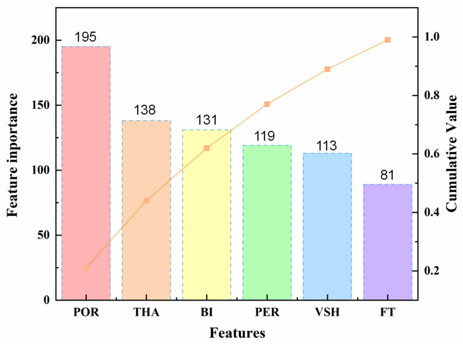
The threshold of 0.6 was selected based on the following considerations: On the one hand, features with grey relational grades greater than 0.6 exhibit relatively strong trend correlations with AOF and can effectively reflect the main controlling factors of AOF. On the other hand, features with grey relational grades lower than 0.6 make relatively weak contributions to the target variable. Further introducing these features may increase model complexity and introduce redundant information, thereby reducing model training efficiency. Therefore, this threshold provides a reasonable balance between retaining the main effective information and reducing redundant inputs. Meanwhile, to verify whether the selected main controlling factors can cover most of the key information influencing AOF, the regression method in LightGBM was used to predict the sweet spots of the target reservoir. The six main controlling factors selected by GRA were used as the inputs of the LightGBM model. In the LightGBM model, the contribution of each feature to the prediction results was evaluated based on the total gain produced when the feature was used as a splitting point across all trees. As shown by the cumulative contribution curve based on the LightGBM feature importance results, the cumulative contribution value continuously increases as the selected features are sequentially introduced according to their importance values in the LightGBM model. After PER, THA, POR, BI, FT, and VSH are included, the cumulative contribution rate reaches a relatively high level. In contrast, the subsequent inclusion of UCS, Ed, Ud, and IGS produces only limited improvement in the cumulative contribution rate. This indicates that the first six features can already represent the main information affecting AOF, while the additional contribution of lower-correlation features to the model results is relatively small. This result further verifies the rationality and effectiveness of using GRA to screen the main controlling factors, as shown in Figure 8.

To further justify the selection of the grey relational grade threshold of 0.6, comparative experiments were conducted using different numbers of input features according to the GRA ranking. Specifically, the top 3, 4, 5, 6, 8, and all 10 features were separately used as inputs for the LightGBM model.

As shown in

Table 4. Prediction performance of the LightGBM model using different numbers of GRA-ranked features.

Feature Subset	Number of Features	Input Features Based on GRA Ranking	MSE	RMSE	R2
Top 3	3	PER, THA, POR	0.2864	0.5352	0.8456
Top 4	4	PER, THA, POR, BI	0.2317	0.4814	0.8794
Top 5	5	PER, THA, POR, BI, FT	0.1989	0.4460	0.8936
Top 6	6	PER, THA, POR, BI, FT, VSH	0.1765	0.4201	0.9233
Top 8	8	PER, THA, POR, BI, FT, VSH, UCS, Ed	0.1808	0.4252	0.9189
All features	10	PER, THA, POR, BI, FT, VSH, UCS, Ed, Ud, IGS	0.1874	0.4329	0.9136

, the model performance improves as the number of input features increases from three to six. The best performance is achieved when the top six features are used, with an MSE of 0.1765, an RMSE of 0.4201, and an R² of 0.9233. However, when the top eight or all ten features are included, the prediction performance does not further improve and even slightly decreases. This indicates that the lower-ranked features provide limited additional information and may introduce redundant information or noise. Therefore, the six features selected using the threshold of 0.6 provide an appropriate balance between prediction accuracy and model complexity.

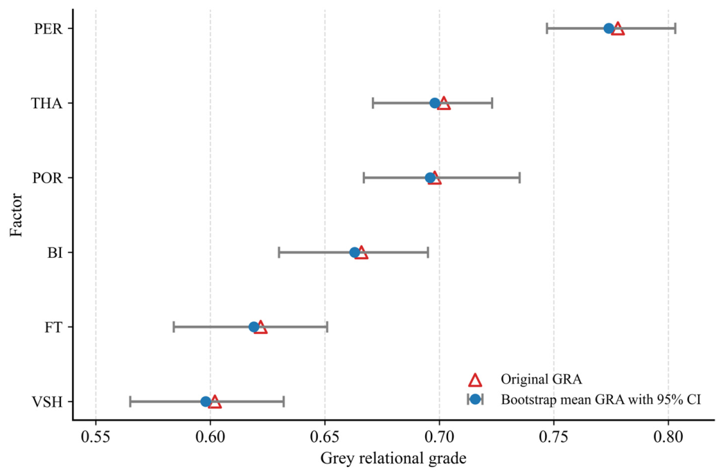
To further assess the statistical stability of the GRA-based feature ranking, a bootstrap resampling analysis was performed. The original dataset was repeatedly resampled with replacement, and the grey relational grade of each factor was recalculated for each bootstrap sample.

The bootstrap mean GRA values are very close to the original GRA values for all selected factors, indicating that the calculated grey relational grades are not highly sensitive to sampling variation. In addition, the 95% confidence intervals are relatively narrow, suggesting that the GRA values remain stable under repeated resampling conditions. Among the selected factors, PER exhibits the highest bootstrap mean GRA and remains clearly separated from the other variables, confirming its dominant influence on AOF. THA and POR show comparable GRA values and consistently rank among the leading factors, while BI, FT, and VSH exhibit slightly lower but still stable grey relational grades. Overall, the bootstrap confidence intervals demonstrate that the GRA-derived feature ranking is robust under sampling variability, providing additional statistical support for the identification of PER, THA, POR, BI, FT, and VSH as the dominant input factors for the subsequent GRA-LightGBM model (see Figure 9).

3.2.2. Sweet Spot Prediction

To develop a reliable sweet spot prediction model for tight gas reservoirs, the hyperparameters of the LightGBM regression model, including min_data_in_leaf, learning_rate, and num_leaves, were optimized. These hyperparameters play important roles in controlling model complexity, learning efficiency, and overfitting risk. In this study, GridSearchCV with three-fold cross-validation was introduced for hyperparameter tuning. A predefined parameter grid was used to traverse different hyperparameter combinations, and the predictive performance of each combination was evaluated through cross-validation [27]. Considering the limited sample size of 56 wells, three-fold cross-validation was adopted to balance validation reliability and training data availability. The parameter grid used in this study is shown in

Table 5. Grid search parameter settings.

Parameter Name	Candidate Values	Rationale for Value Range Selection	Function
min_data_in_leaf	[20, 30, 40]	Balances model complexity and overfitting risk	Prevents overfitting by controlling the minimum data size in leaf nodes
learning_rate	[0.01, 0.03, 0.05]	Explores trade-offs between convergence speed and model accuracy	Controls the step size during model training iterations
num_leaves	[31, 63, 127]	Ensures more regular and balanced tree structures for efficient training and computation	Determines the model’s complexity by setting the number of leaves in each tree

. The optimal hyperparameter combination was then used to train the final LightGBM model, and its predictive performance was evaluated on the test set.

The candidate parameter values were selected based on empirical knowledge, theoretical analysis, and comprehensive consideration of model performance. By conducting experiments and fine-tuning within these candidate values, the most suitable parameter combination for hydraulic fracturing sweet spot prediction can be identified, thereby enhancing model performance and generalization capability. GridSearchCV exhaustively explores all combinations of num_leaves (31/63/127), learning_rate (0.01/0.03/0.05), and min_data_in_leaf (20/30/40), ultimately selecting the configuration that minimizes the validation error from a total of twenty-seven candidate combinations (

Table 6. Optimal hyperparameter combination.

Min_Data_in_Leaf	Learning_Rate	num_Leaves
20	0.05	31

). This exhaustive search strategy ensures comprehensive coverage of the parameter space, while the integration of cross-validation helps mitigate overfitting risks, leading to more robust hyperparameter selection for the model.

4. Results

4.1. Prediction Performance of the Proposed GRA-LightGBM Model

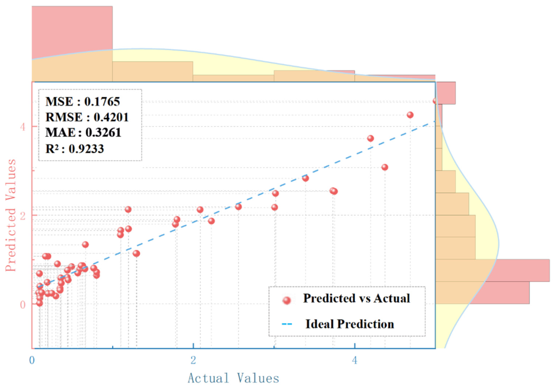
To evaluate the effectiveness of the constructed tight gas reservoir sweet spot prediction model, the dataset comprising 56 wells was divided into a training set and a testing set at a ratio of 8:2. Specifically, data from 44 wells were used to train the model. After training, the model was used to predict the absolute open flow (AOF) based on the average-value dataset of individual fracturing intervals from the remaining 12 testing wells. The predicted values were then compared with the actual values to validate the predictive performance of the model, as shown in Figure 10.

The proposed model’s predictive performance was evaluated using four key performance metrics. The first is the Mean Squared Error (MSE), which reflects the overall squared deviation between the predicted and actual values and is more sensitive to large prediction errors. As shown in Figure 10, the final MSE value is 0.1765, indicating a relatively low prediction error. The second metric is the Root Mean Squared Error (RMSE), which is calculated as the square root of the average squared prediction error and measures the average discrepancy between predicted and actual values in the same unit as the target variable. The final RMSE is 0.4201, further suggesting that the model maintains a relatively low prediction error. The third metric is the Mean Absolute Error (MAE), which measures the average absolute difference between the predicted and actual values and provides a direct indication of the overall prediction error. The final MAE value is 0.326, indicating that the average absolute prediction error of the model is relatively small. The model also achieved a coefficient of determination (R²) of 0.9233, with values closer to 1 indicating stronger explanatory power. This result suggests that the model can explain approximately 92.33% of the variance in the observed AOF data, indicating good agreement between the predicted and measured values and favorable predictive performance.

It is observed that predictions within the AOF range of 0–2 exhibit higher accuracy and denser data points. This is attributed to strong heterogeneity in the target reservoir and uneven parameter distribution. The majority of the original data samples fall within this range, enabling the model to learn effectively and enhance predictive accuracy. In contrast, in the 2–5 range, limited data availability results in lower training precision, leading to greater discrepancies between predicted and actual values.

4.2. Robustness and Generalization Evaluation Under Limited Sample Conditions

4.2.1. Learning Curve Analysis

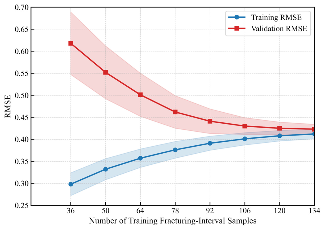
To further investigate the influence of sample size on model performance and to evaluate the potential overfitting behavior of the proposed GRA-LightGBM model, a learning-curve analysis was conducted. Although the dataset was obtained from 56 wells, each well may contain multiple fracturing intervals; therefore, the learning curve was constructed using the number of fracturing-interval samples as the horizontal axis. The training and validation RMSE values were calculated under different training sample sizes, and the corresponding standard deviations were used to represent the uncertainty of model performance. The learning curve is shown in Figure 11.

As shown in Figure 11, the validation RMSE decreases continuously from 0.618 to 0.423 as the number of training fracturing-interval samples increases from 36 to 64, indicating that the model benefits from additional training samples and gradually improves its generalization capability. In contrast, the training RMSE slightly increases from 0.298 to 0.412 and then tends to stabilize. This trend is reasonable because a small training set can be more easily fitted by the model, whereas larger training sets introduce greater geological and engineering heterogeneity, making the training task more challenging. Meanwhile, the gap between the training and validation RMSE curves becomes progressively smaller with increasing training sample size. When the number of training fracturing-interval samples reaches 134, the training RMSE and validation RMSE are 0.412 and 0.423, respectively, showing only a small difference. This convergence suggests that the proposed GRA-LightGBM model does not exhibit severe overfitting.

4.2.2. Five-Fold Cross-Validation

To address the potential limitation of relying on a single train–test split, five-fold cross-validation was further performed to evaluate the robustness and generalization capability of the proposed GRA-LightGBM model under limited sample conditions. In addition to the original division of 44 wells for training and 12 wells for independent testing, the 56 well samples were randomly divided into five approximately equal-sized subsets for cross-validation. In each validation round, four subsets were used for model training, while the remaining subset was used for validation. This process was repeated five times so that each subset served once as the validation set. The prediction performance of each fold was evaluated using MSE, RMSE, and R². The mean and standard deviation of these metrics were then calculated to quantify the average predictive accuracy and the stability of the model across different data partitions. The five-fold cross-validation results are summarized in

Table 7. Five-fold cross-validation results of the proposed GRA-LightGBM model.

Fold	MSE	RMSE	R2
Fold 1	0.1682	0.4101	0.9284
Fold 2	0.1847	0.4298	0.9146
Fold 3	0.1735	0.4165	0.9218
Fold 4	0.1913	0.4374	0.9067
Fold 5	0.1789	0.4230	0.9185
Mean	0.1793	0.4234	0.9180
SD	0.0090	0.0106	0.0081

.

As shown in Table 7, the five-fold cross-validation results demonstrate that the proposed GRA-LightGBM model maintains stable predictive performance under different data partitions. The mean MSE, RMSE, and R² values were 0.1793, 0.4234, and 0.9180, respectively, with corresponding standard deviations of 0.0090, 0.0106, and 0.0081. The relatively small standard deviations indicate that the model performance fluctuated only slightly across the five folds, suggesting that the prediction results are not strongly dependent on a specific train–test split.

4.3. Comparative Evaluation with Benchmark Models

4.3.1. Comparison with Traditional Machine Learning Models

To evaluate the predictive performance of the proposed GRA-LightGBM model, four commonly used traditional machine learning models were selected as benchmark models, namely Back Propagation Neural Network (BPNN) [28], K-Nearest Neighbors (KNN) [29], Ridge Regression [30], and Linear Regression (LR) [31]. These models were chosen to provide comparisons from different modeling perspectives. LR and Ridge Regression represent linear regression methods, with Ridge Regression introducing L2 regularization to reduce the influence of multicollinearity. KNN is a non-parametric learning method that predicts target values based on the similarity of neighboring samples, while BPNN is a typical nonlinear neural network model with the ability to approximate complex relationships. By comparing these models under the same dataset and evaluation conditions, the prediction accuracy and nonlinear fitting capability of GRA-LightGBM can be more comprehensively assessed.

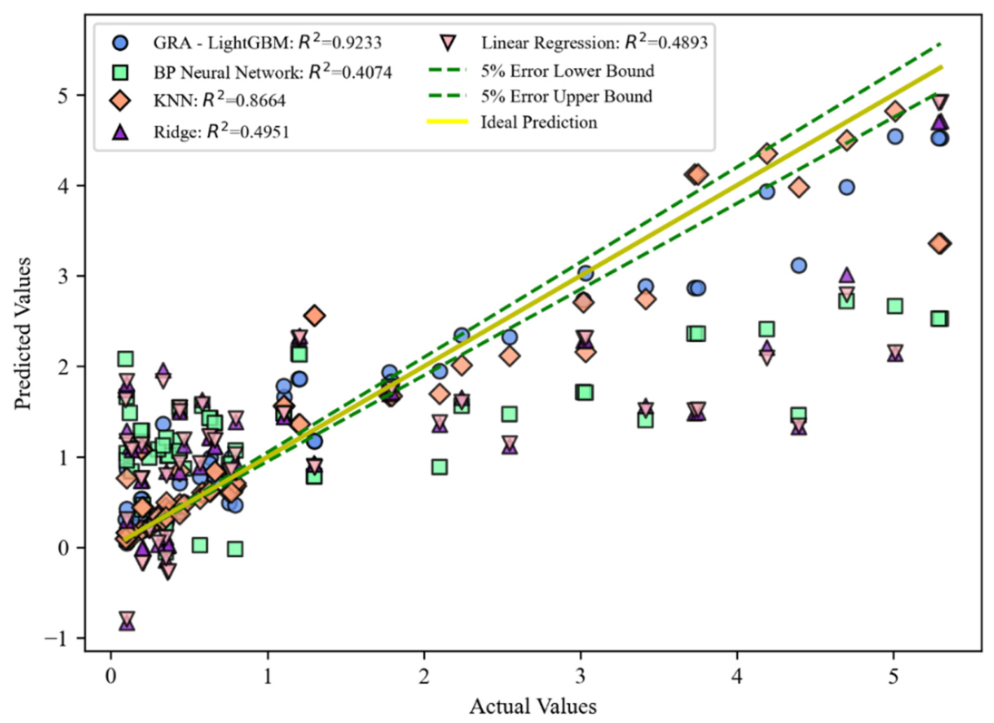
As shown in Figure 12, the predicted values of GRA-LightGBM are more closely distributed around the ideal prediction line than those of the other benchmark models. Most of the GRA-LightGBM prediction points fall near or within the ±5% error bounds, indicating that the proposed model can accurately capture the variation trend of AOF. The model achieves the highest R² value of 0.9233, suggesting that approximately 92.33% of the variance in the observed AOF values can be explained by GRA-LightGBM. In contrast, the prediction points of LR and Ridge Regression show obvious dispersion, especially for samples with medium and high AOF values. Their R² values are 0.4893 and 0.4951, respectively, indicating that linear models have limited ability to describe the complex nonlinear relationship between geological–engineering parameters and AOF. Although Ridge Regression introduces L2 regularization, its improvement over LR is limited, suggesting that the main challenge in this prediction task is not only multicollinearity but also nonlinear feature–target relationships. BPNN obtains an R² value of 0.4074, which is lower than that of the other models. This may be related to the limited sample size of the dataset. Neural network models usually require sufficient training samples to learn stable nonlinear mapping relationships. Under small-sample conditions, BPNN may suffer from unstable training or insufficient generalization, leading to large deviations in AOF prediction. KNN performs better than LR, Ridge Regression, and BPNN, with an R² value of 0.8664, indicating that local similarity-based prediction can capture part of the nonlinear characteristics in the dataset. However, its prediction points are still more scattered than those of GRA-LightGBM, particularly in the high-AOF range, suggesting that KNN is sensitive to sample distribution and may have limited extrapolation ability. Overall, GRA-LightGBM shows the most accurate and stable prediction performance among all compared models. This advantage can be attributed to the combination of GRA-based feature selection and the strong nonlinear fitting ability of LightGBM. GRA helps identify the most relevant input variables and reduce redundant feature information, while LightGBM effectively captures nonlinear interactions through gradient boosting decision trees. Therefore, the proposed GRA-LightGBM model is more suitable for AOF prediction and can provide more reliable support for fracturing sweet spot identification in tight gas reservoirs.

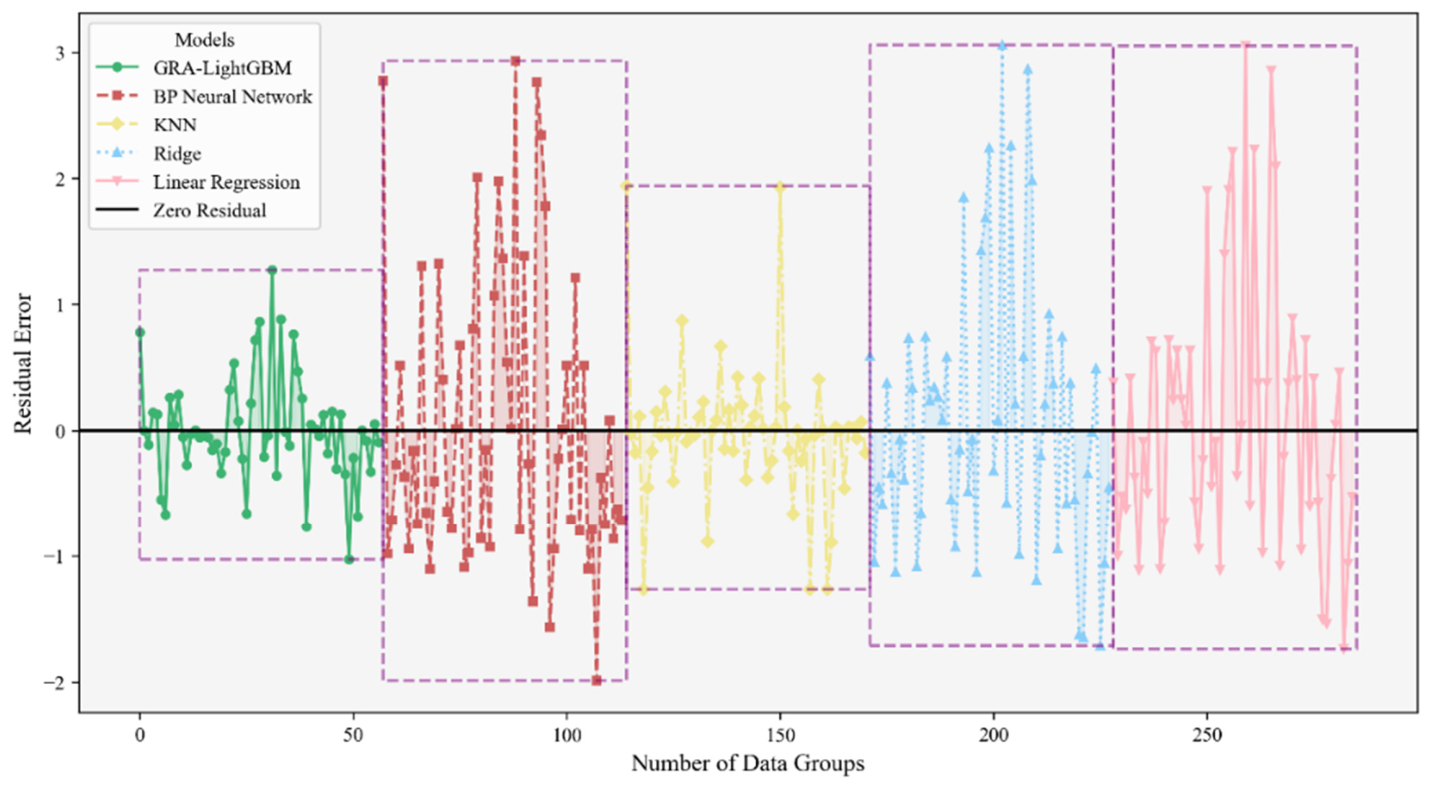
In addition to the predicted-versus-actual comparison, residual error analysis was conducted to further evaluate the prediction bias and stability of different models. The residual error was calculated as the difference between the predicted and actual AOF values. A residual distribution closer to the zero-residual line indicates smaller prediction deviation and better model stability. Therefore, the residual distributions of GRA-LightGBM, BPNN, KNN, Ridge Regression, and Linear Regression were compared to assess the reliability of different models in AOF prediction.

As shown in Figure 13, GRA-LightGBM presents the most concentrated residual distribution around the zero-residual line, with the smallest fluctuation range among all compared models. This indicates that the proposed model can generate predictions with lower bias and higher stability. In contrast, BPNN exhibits large residual fluctuations, which may be associated with unstable learning under limited sample conditions. KNN shows relatively better residual control than BPNN, but its residuals remain more dispersed than those of GRA-LightGBM, suggesting that local similarity-based prediction is sensitive to sample distribution. Ridge Regression and Linear Regression show larger deviations from the zero-residual line, indicating that linear models are insufficient for describing the nonlinear relationship between input parameters and AOF. These residual patterns further confirm that GRA-LightGBM provides more accurate and stable AOF predictions than the traditional benchmark models. The improved residual behavior can be attributed to the GRA-based feature selection strategy, which reduces redundant feature information, and the nonlinear ensemble learning capability of LightGBM, which enhances the modeling of complex feature interactions.

4.3.2. Comparison with Tree-Based Ensemble Models

To further evaluate the effectiveness of the proposed GRA-LightGBM model, several representative tree-based machine learning models were selected as benchmark models for comparative experiments, including Random Forest, Extra Trees, XGBoost, CatBoost, and the original LightGBM. These models are widely used ensemble learning algorithms and have shown strong performance in nonlinear regression tasks. Random Forest and Extra Trees were introduced as bagging-based ensemble models, while XGBoost, CatBoost, and LightGBM were selected as boosting-based models. By comparing GRA-LightGBM with these benchmark models under the same dataset and evaluation criteria, the contribution of the GRA-based feature selection strategy to the predictive performance of LightGBM can be further assessed.

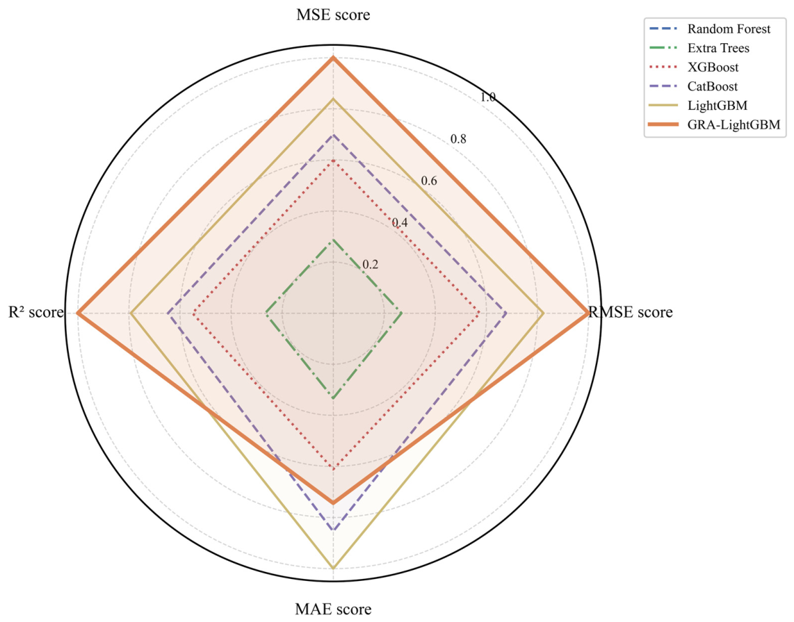
As illustrated in Figure 14, the compared tree-based models show different predictive capabilities across the four normalized evaluation metrics. Random Forest and Extra Trees obtain relatively lower scores, particularly in MSE, RMSE, and R², indicating that their prediction accuracy and goodness of fit are weaker than those of the boosting-based models. XGBoost and CatBoost show improved performance compared with the bagging-based models, reflecting their stronger ability to model nonlinear relationships in the AOF dataset. Among the original benchmark models, LightGBM exhibits the most competitive performance and achieves the highest normalized score for MAE, suggesting its advantage in controlling average absolute prediction error. Compared with the benchmark models, the proposed GRA-LightGBM achieves the highest normalized scores for MSE, RMSE, and R², demonstrating its superiority in reducing squared prediction errors and improving the overall fitting capability. Although its MAE score is slightly lower than that of the original LightGBM, GRA-LightGBM presents the best overall performance across the four evaluation metrics. This result confirms that the GRA-based feature selection strategy can further enhance LightGBM by improving the quality of input features and reducing redundant information, thereby increasing the robustness and predictive accuracy of AOF prediction.

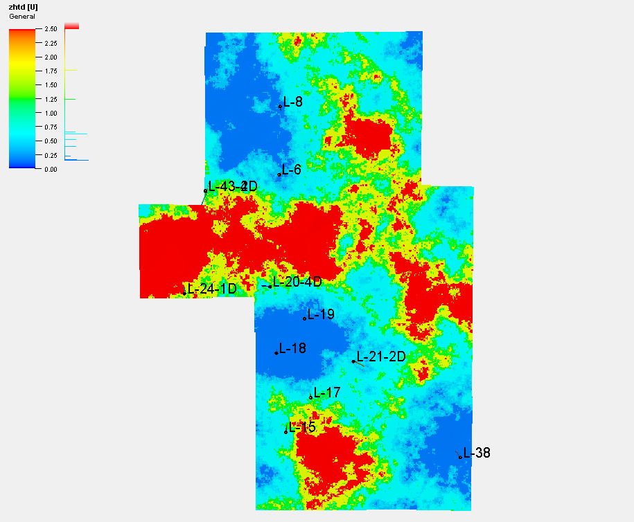
Based on the Petrel integrated exploration and development platform, the predicted values from the model were imported into the geological model of the Linxingdong study area to quantitatively characterize the distribution pattern of sweet spots in the region (Figure 15). The results indicate that the reservoir in the Linxingdong area exhibits strong heterogeneity, with an uneven distribution of sweet spots. The sweet spots are mainly concentrated in the northwestern region, where hydrocarbon enrichment is significant and development potential is high. These findings provide a visual and quantitative basis for reservoir evaluation and development decision-making.

5. Conclusions

This study proposed a GRA-LightGBM model for predicting and characterizing fracturing sweet spots in tight gas reservoirs. The model integrates Grey Relational Analysis with LightGBM, in which GRA is used to identify dominant factors closely related to AOF, and LightGBM is then employed to construct a nonlinear prediction model. This workflow improves the quality of input features and enhances the ability of the model to capture complex relationships between geological–engineering parameters and reservoir productivity.

The results show that the proposed GRA-LightGBM model achieves high prediction accuracy in the Linxing East study area, with an R² value of 0.9233. The predicted values are closely distributed around the ideal prediction line, and the residuals are mainly concentrated near the zero-residual line, indicating good prediction accuracy and stability. Compared with traditional machine learning models, including BPNN, KNN, Ridge Regression, and Linear Regression, GRA-LightGBM shows smaller prediction deviations and stronger nonlinear fitting capability. Additional comparisons with tree-based ensemble models, including Random Forest, Extra Trees, XGBoost, CatBoost, and standard LightGBM, further demonstrate the superiority of the proposed model. GRA-LightGBM achieves the best overall performance, with the highest normalized scores for MSE, RMSE, and R². These results confirm that GRA-based feature selection can effectively improve the predictive robustness and accuracy of LightGBM.

Based on the prediction results, the spatial distribution of fracturing sweet spots was visualized using the Petrel platform, providing practical support for reservoir evaluation and well deployment optimization. Overall, the proposed GRA-LightGBM workflow integrates dominant factor identification, nonlinear AOF prediction, and sweet spot spatial characterization, offering an effective tool for tight gas reservoir development.

Some limitations remain in this study. The GRA-based feature selection process may be affected by the weighting strategy, and the model performance depends on the quality and representativeness of the dataset. Future work should incorporate multi-source data fusion, adaptive weighting mechanisms, uncertainty analysis, and transfer learning to further improve the generalization ability and robustness of the model in complex tight gas reservoir settings.

References

1. Zhu, H.; Gong, D.; Zhang, B. A multi-scale geological-engineering sweet spot evaluation method for tight sandstone gas reservoirs. Nat. Gas Ind. B 2023, 10, 522–532. [Google Scholar]
2. Wang, W.; Lin, C.; Zhang, X. Evaluation of sweet spots for a tight sandstone reservoir: A quantitative study of diagenesis in the fourth member of the Oligocene Huagang Formation, Xihu Depression, East China Sea Shelf Basin. Mar. Pet. Geol. 2024, 163, 106799. [Google Scholar] [CrossRef]
3. Shi, C.; Bo, T.; Xie, B. A double-sweet-spot-based evaluation method for shale reservoir fracability. J. Shenzhen Univ. 2024, 41, 184–191. [Google Scholar]
4. Zhang, W.; Xiao, Z.; Yi, H.; Jiang, M.; Zhu, Y. Application of the “double sweet spot” identification method for tight sandstone reservoirs in the Paleogene reservoirs of the Lufeng area, eastern South China Sea. Pet. Geophys. Prospect. 2024, 63, 217–228. [Google Scholar]
5. Yang, K.; Luo, S.; Hua, L.; Tang, H.; Sun, Z. Study on fracturing sweet spot prediction of tight conglomerate reservoirs: A case study of the Ma-18 well area. Sci. Technol. Eng. 2022, 22, 14174–14183. [Google Scholar]
6. Ouenes, A.; Zellou, A.; Basinski, P.M.; Head, C.F. Practical Use of Neural Networks in Tight Gas Fractured Reservoirs: Application to the San Juan Basin. In Proceedings of the SPE Rocky Mountain Regional/Low-Permeability Reservoirs Symposium, Denver, CO, USA, 5–8 April 1998; p. 573. [Google Scholar] [CrossRef]
7. Bakay, A.; Caers, J.; Mukerji, T.; Dong, Y.; Briceno, A.; Neumann, D. Integrating Geostatistical Modeling with Machine Learning for Production Forecast in Shale Reservoirs: Case Study from Eagle Ford. In Proceedings of the 7th Unconventional Resources Technology Conference, American Association of Petroleum Geologists, Denver, CO, USA, 22–24 July 2019; pp. 4370–4385. [Google Scholar] [CrossRef]
8. Liu, F. Application of machine learning in geological reservoir sweet spot prediction. Master’s Thesis, China University of Petroleum (East China), Shandong, China, 2023. [Google Scholar]
9. Algarhy, A.; Ibrahim, A.F. Application of Machine Learning to Predict the Organic Shale Sweet-Spot Quality Index. In Proceedings of the SPE Eastern Regional Meeting, Wheeling, WV, USA, 18–20 October 2022; p. SPE-211889-MS. [Google Scholar] [CrossRef]
10. Algarhy, A.; Ibrahim, A.F.; Gabry, M.A.; Ali, A.G. Predicting Shale Production Performance Through Machine Learning: The Development and Application of the Sweet Spot Quality Index. In Proceedings of the SPE Eastern Regional Meeting, Wheeling, WV, USA, 3–5 October 2023; p. SPE-215911-MS. [Google Scholar] [CrossRef]
11. Han, K. Research and application of shale oil sweet spot prediction method based on big data technology. Master’s Thesis, Yangtze University, Jingzhou, China, 2024. [Google Scholar]
12. Yang, D. Intelligent prediction of geological sweet spots in Jimusar shale oil based on seismic attributes. Master’s Thesis, China University of Petroleum, Beijing, China, 2023. [Google Scholar]
13. Deng, Y.; Wang, W.; Du, X.; Su, Y.; Sun, S.; Jia, F.; Jiang, Z. An Automated Data-Driven Workflow for Identifying Fractured Horizontal Well Sweet Spots in Shale Reservoirs. In Proceedings of the 57th U.S. Rock Mechanics/Geomechanics Symposium, Atlanta, GA, USA, 25–28 June 2023; p. ARMA-2023-0672. [Google Scholar] [CrossRef]
14. Jiang, F.; Hu, M.; Hu, T.; Lyu, J.; Huang, L.; Liu, C.; Jiang, Z.; Huang, R.; Zhang, C.; Wu, G.; et al. Controlling factors and models of shale oil enrichment in Lower Permian Fengcheng Formation, Mahu Sag, Junggar Basin, NW China. Pet. Explor. Dev. 2023, 50, 812–825. [Google Scholar] [CrossRef]
15. Liu, G.; Liu, H.; Xian, B.; Gao, D.; Wang, X.; Zhang, Z. Fuzzy pattern recognition model of geological sweet spot for coalbed methane development. Pet. Explor. Dev. 2023, 50, 924–933. [Google Scholar]
16. Xiao, X.; Yan, J.; Guo, W. Sweet spot parameter prediction method for shale gas reservoirs based on the LightGBM algorithm. China Coal Geol. 2023, 35, 29–37. [Google Scholar]
17. Guolin, K.; Qi, M.; Finley, T.; Wang, T.; Chen, W.; Ma, W.; Ye, Q.; Liu, T.-Y. LightGBM: A Highly Efficient Gradient Boosting Decision Tree. In Proceedings of the 31st Conference on Neural Information Processing Systems, Long Beach, CA, USA, 4–9 December 2017; pp. 3149–3157. [Google Scholar]
18. Agrawal, R.J.; Shanahan, J.G. Location disambiguation in local searches using gradient boosted decision trees. In Proceedings of the 18th SIGSPATIAL International Conference on Advances in Geographic Information Systems, San Jose, CA, USA, 2–5 November 2010; pp. 129–136. [Google Scholar] [CrossRef]
19. Zhan, Z.-H.; You, Z.-H.; Li, L.-P.; Zhou, Y.; Yi, H.-C. Accurate prediction of ncRNA-protein interactions from the integration of sequence and evolutionary information. Front. Genet. 2018, 9, 458. [Google Scholar] [PubMed]
20. Liang, W.; Luo, S.; Zhao, G.; Wu, H. Predicting hard rock pillar stability using GBDT, XGBoost, and LightGBM Algorithms. Mathematics 2020, 8, 765. [Google Scholar] [CrossRef]
21. Liu, G.; Li, Y.; Wang, X. Expedited tensor program compilation based on LightGBM. J. Phys. Conf. Ser. 2021, 1, 1–10. [Google Scholar]
22. Wang, W.; Dang, H.; Kang, S.; Xiao, Q.; Ding, L.; Shi, L. Porosity prediction of tight oil reservoirs based on LightGBM and SHAP algorithms. Pet. Geol. Recovery Effic. 2025, 32, 90–99. [Google Scholar]
23. Liu, S.; Yang, Y.; Cao, Y.; Xie, N. A summary on the research of GRA models. Grey Syst. Theory Appl. 2013, 3, 7–15. [Google Scholar] [CrossRef]
24. Luo, Y.; Xu, Q.; Li, W.; Jiang, F.; Xiao, B. A multi-step decision prediction model based on LightGBM. Grey Syst. Theory Appl. 2021, 3, 5714–5718. [Google Scholar] [CrossRef]
25. Xia, H.; Lai, J.; Li, G. Sweet spot prediction of shale oil reservoirs based on well-logging data. J. Southwest Pet. Univ. Nat. Sci. Ed. 2021, 43, 200–207. [Google Scholar]
26. Yang, H.; Li, F.; Wang, W.; Fu, Y.; Tang, Q.; Yang, J.; Xie, B. A novel approach for identifying sweet spots in tight reservoir fracturing engineering based on physical-data dual drive. J. Appl. Geophys. 2025, 238, 105735. [Google Scholar] [CrossRef]
27. Alhakeem, Z.M.; Jebur, Y.M.; Henedy, S.N.; Imran, H.; Bernardo, L.F.A.; Hussein, H.M. Prediction of Ecofriendly Concrete Compressive Strength Using Gradient Boosting Regression Tree Combined with GridSearchCV Hyperparameter-Optimization Techniques. Materials 2022, 15, 7432. [Google Scholar] [PubMed]
28. Buscema, M. Back Propagation Neural Networks. Subst. Use Misuse 1998, 33, 233–270. [Google Scholar] [CrossRef] [PubMed]
29. Zhang, Z. Introduction to machine learning: K-nearest neighbors. Ann. Transl. Med. 2016, 4, 218. [Google Scholar] [CrossRef] [PubMed]
30. McDonald, G.C. Ridge regression. WIREs Comput. Stat. 2009, 1, 93100. [Google Scholar] [CrossRef]
31. Su, X.; Yan, X.; Tsai, C.-L. Linear regression. WIREs Comput. Stat. 2012, 4, 275–294. [Google Scholar] [CrossRef]
Figure 1. Core algorithmic flow of the LightGBM model. Feature processing stores raw data with numeric types, builds histograms via binning, and trains leaf-wise decision trees with residual updates. Final outputs are aggregated into the model.
Processes 14 02160 g001
Figure 2. Computational Workflow of Grey Relational Analysis (GRA). The process involves normalization of the input data, computation of correlation coefficients, calculation of the correlation degree, and ranking of feature relevance based on their relational closeness to the control variable.
Processes 14 02160 g002
Figure 3. Structural diagram of the GRA-LightGBM prediction model. Principal controlling factors are identified using GRA and subsequently input into the LightGBM model. Through a leaf-wise tree growth strategy, decision trees are trained sequentially by minimizing residuals and cumulatively generating the final prediction.
Processes 14 02160 g003
Figure 4. Methodological workflow diagram. The process includes geological and engineering data acquisition, preprocessing and normalization, feature selection using GRA, model training with LightGBM, prediction of sweet spots, and visualization of predicted zones using Petrel 2021.
Processes 14 02160 g004
Figure 5. Relationships between engineering and geological parameters and AOF. Correlation scatter plots showing the relationship between various features (POR, PER, IGS, VSH, THA, Ed, Ud, BI, UCS, and FT) and the target variable AOF. Each subplot contains data points, a fitted line, and a 99% confidence ellipse around the mean.
Processes 14 02160 g005
Figure 6. Variation in grey relational grades for different influencing factors under distinguishing coefficients ρ = 0.3, 0.4, 0.5, 0.6, and 0.7. 3D bar chart illustrating the correlation degree between different features and the target variable, with different colors representing various correlation coefficients (rho values ranging from 0.3 to 0.7).
Processes 14 02160 g006
Figure 7. Grey relational grades between evaluation parameters and AOF at a distinguishing coefficient of 0.5. Bar chart displaying the correlation degree of different features (PER, THA, POR, BI, FT, VSH, UCS, Ed, Ud, and IGS) with the target variable. The height of each bar represents the correlation coefficient value.
Processes 14 02160 g007
Figure 8. Cumulative trend of feature importance in the LightGBM model. Bars indicate the number of features; the line shows cumulative importance. As POR, THA, BI, PER, VSH, and FT are added, the cumulative value approaches 1, indicating the key features accounting for the model’s primary explanatory power.
Processes 14 02160 g008
Figure 9. Bootstrap-based confidence intervals of grey relational grades for the selected dominant factors. The blue circles represent the bootstrap mean GRA values, the grey error bars indicate the 95% confidence intervals, and the red hollow triangles denote the original GRA values.
Processes 14 02160 g009
Figure 10. Comparison between actual and predicted AOF values. It includes metrics such as MSE (0.1765), RMSE (0.4201), and R2 (0.9233). The red dots are the predicted vs. actual data points, and the blue dashed line represents the ideal prediction. The orange and red bars in the marginal histograms are used only for visualizing the distributions of actual and predicted values and do not represent additional categories.
Processes 14 02160 g010
Figure 11. Learning curve of the proposed GRA-LightGBM model based on fracturing-interval samples. The curves show the variation in training and validation RMSE with increasing training sample size, and the shaded areas denote one standard deviation. The convergence of the two curves indicates stable model performance and limited overfitting.
Processes 14 02160 g011
Figure 12. Comparative validation of multiple models. Different colored dots represent various models (GRA-LightGBM, BP Neural Network, KNN, Ridge, and Linear Regression), with their respective R2 values shown. The green dashed lines are the 5% error bounds, and the yellow line is the ideal prediction.
Processes 14 02160 g012
Figure 13. Residual distribution diagram. The horizontal axis denotes the number of data groups, and the vertical axis represents residuals. The black baseline indicates zero residual. The GRA-LightGBM model shows the smallest residual fluctuation, indicating minimal prediction error and higher stability.
Processes 14 02160 g013
Figure 14. Radar chart of normalized performance scores for different tree-based models. MSE, RMSE, and MAE were inversely normalized because lower values indicate better predictive performance, whereas R2 was directly normalized. Therefore, a larger normalized score represents better model performance.
Processes 14 02160 g014
Figure 15. Sweet spot distribution in the Linxingdong study block. Sweet spot values range from 0 to 2.5, with higher values indicating better quality. In the Linxingdong block, sweet spots are unevenly distributed, with high-quality fracturing zones predominantly located in the northwest.
Processes 14 02160 g015