Healthy-State Performance Modeling of a Multistage Natural Gas Centrifugal Compressor Using a CFD-Generated Baseline and Factory-Data Correction

Abstract

Accurate healthy-state performance modeling under multiple operating conditions is essential for the condition assessment of industrial centrifugal compressors. However, conventional healthy-state baselines often struggle to meet the requirements of real-time condition assessment for centrifugal compressors operating under complex real-gas and multi-condition environments. To address this issue, this study proposes a two-layer framework combining a CFD-based physical baseline with data-driven residual correction using limited factory data. A three-dimensional full-machine CFD model was reconstructed and validated under real-gas conditions, then used to generate 1440 healthy-state operating points. XGBoost, LightGBM, Random Forest, and multilayer perceptron were evaluated as baseline surrogate models. A residual-correction model was subsequently trained to compensate for systematic discrepancies between CFD predictions and actual machine performance. Ablation tests compared the CFD baseline, a factory-data-only model, and the proposed hybrid model. Online computation requires only surrogate inference and residual correction, achieving an inference latency of 0.6585 ms per operating point on Intel64 Family, compatible with the 60 s SCADA sampling interval. After correction, the maximum errors in power, polytropic head, and polytropic efficiency were 0.611%, 0.481%, and 0.899%, respectively. Post-overhaul field validation yielded maximum errors of 1.650%, 3.048%, and 1.708% for outlet pressure, power, and polytropic efficiency. The framework provides a physically grounded and computationally efficient healthy-state reference, although its transferability requires validation using additional station-specific data.

1. Introduction

Natural gas pipeline transportation is one of the most important modes of long-distance energy delivery because of its large capacity, high stability, and strong safety [1]. In large-scale transmission systems, centrifugal compressors are indispensable for compensating pressure loss [2], maintaining flow continuity, and improving operational efficiency [3]. However, the operating performance of industrial centrifugal compressors is affected simultaneously by gas composition [4], inlet thermodynamic state [5], environmental conditions [6], and load variation [7]. As a result, field monitoring data alone cannot directly reflect the intrinsic health status of the machine. In engineering practice, a newly manufactured compressor or a compressor immediately after major overhaul can usually be regarded as being in a healthy state, whereas long-term service may lead to wear, fouling, leakage, and other degradation phenomena. Therefore, establishing a reliable healthy-state baseline is a prerequisite for quantitative condition assessment.

The core challenge is that the actual measured performance under field conditions is strongly coupled with operating-condition variation. Changes caused by inlet pressure, inlet temperature, rotational speed, and flow rate are superimposed on changes caused by physical degradation, making it difficult to distinguish whether a deviation is induced by off-design operation or by deterioration of the machine itself. Traditional empirical models are often insufficient for such tasks because the thermal performance of industrial centrifugal compressors is highly nonlinear and depends on both internal flow physics and external operating conditions. High-accuracy healthy-state modeling is therefore important not only for equipment condition assessment [8] and fault warning [9] but also for digital twins [10], intelligent pipeline regulation [11], and the integration of physical mechanisms with artificial intelligence [12].

Existing studies on centrifugal-compressor performance can generally be grouped into two major streams: physics-based investigations and data-driven modeling. The first stream mainly relies on CFD simulations and experiments to analyze internal flow structures, heat transfer, aerodynamic losses, and structural optimization [13]. These studies have substantially advanced the understanding of blade loading, diffuser behavior, casing heat transfer, and local transport mechanisms, and have demonstrated the value of high-fidelity numerical tools for compressor design improvement and mechanism interpretation [14,15]. Representative examples include investigations of blade-number effects [16], ported-shroud configurations [17], outlet-duct structures [18], diffuser heat-transfer behavior [19], and conjugate heat-transfer enhancement [20], all of which confirmed that localized geometric or thermal modifications can lead to measurable gains in pressure ratio, efficiency, or operating range. At the same time, turbomachinery performance maps have also been established in the literature using CFD simulations and experimental data [21,22]. However, many of these studies remain focused on single-stage compressors, individual components, simplified configurations, or design-oriented optimization tasks. As a result, they are more suitable for mechanism analysis, performance evaluation, or map construction under specific conditions than for directly supporting healthy-state baseline modeling of full-machine industrial compressors operating under multiple conditions and real-gas environments. The second stream is based on data-driven methods [23,24], where empirical correlations, similarity concepts, experiments, and machine learning algorithms are combined to build performance-prediction models. For instance, Giraldi [25], Bao [26] and Zhang [27] respectively established prediction models based on industrial environments, experimental data and loss mechanisms. Among them, the model established by Zhang [27] had a total pressure ratio RMSE of only 3.47%. On this basis, Peng et al. [28] effectively improved the nonlinear prediction accuracy by integrating gray theory and radial basis function neural networks, and controlled the error within 2.34%. These approaches offer clear advantages in computational efficiency and online prediction capability, and they have shown promising accuracy in practical applications such as sustainability evaluation, performance-parameter prediction, and loss-related model construction. Nevertheless, most existing data-driven models depend strongly on the quantity and representativeness of measured data, while their physical interpretability and extrapolation robustness remain limited when they are applied to industrial full-machine compressors operating in complex real-gas and multi-condition environments. In particular, when healthy-state field data are scarce, purely data-driven approaches often lack a sufficiently reliable physical baseline.

Although CFD-assisted data generation and machine learning surrogate modeling have been widely used in turbomachinery research, most existing studies are primarily oriented toward aerodynamic design, component-level optimization, or performance-map interpolation. Their direct use as a healthy-state reference for in-service full-machine industrial compressors remains limited, especially when the compressor operates with real natural gas under multiple inlet pressures, inlet temperatures, rotational speeds, and flow rates. The contribution of this study is therefore not the generic combination of CFD and machine learning, but the development and validation of a practical two-layer healthy-state baseline framework for a multistage natural-gas centrifugal compressor. The framework first uses a validated full-machine real-gas CFD model to generate an offline physics-based healthy database and then introduces a factory-data residual-correction layer to compensate for systematic differences between the CFD baseline and the actual machine.

The remainder of this paper is organized as follows. Section 2 introduces the full-machine CFD model, thermodynamic performance definitions, and numerical validation. Section 3 presents the construction of the CFD-generated healthy-state baseline model, the factory-data residual-correction framework, and the interpretability analysis. Section 4 validates the final model using post-overhaul field data. 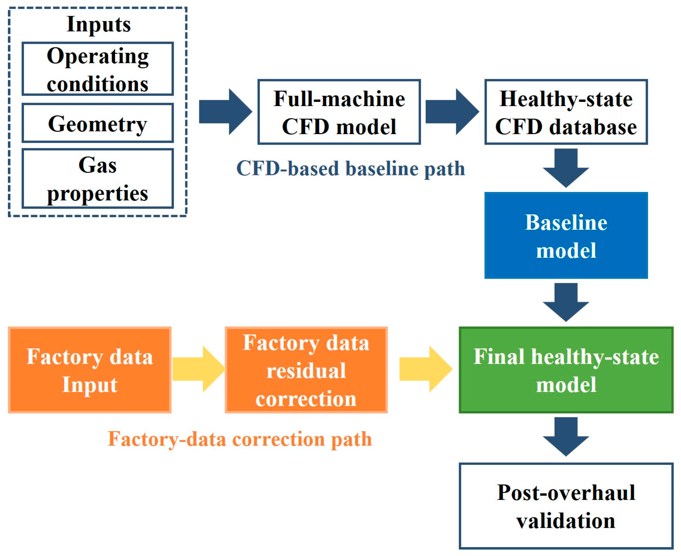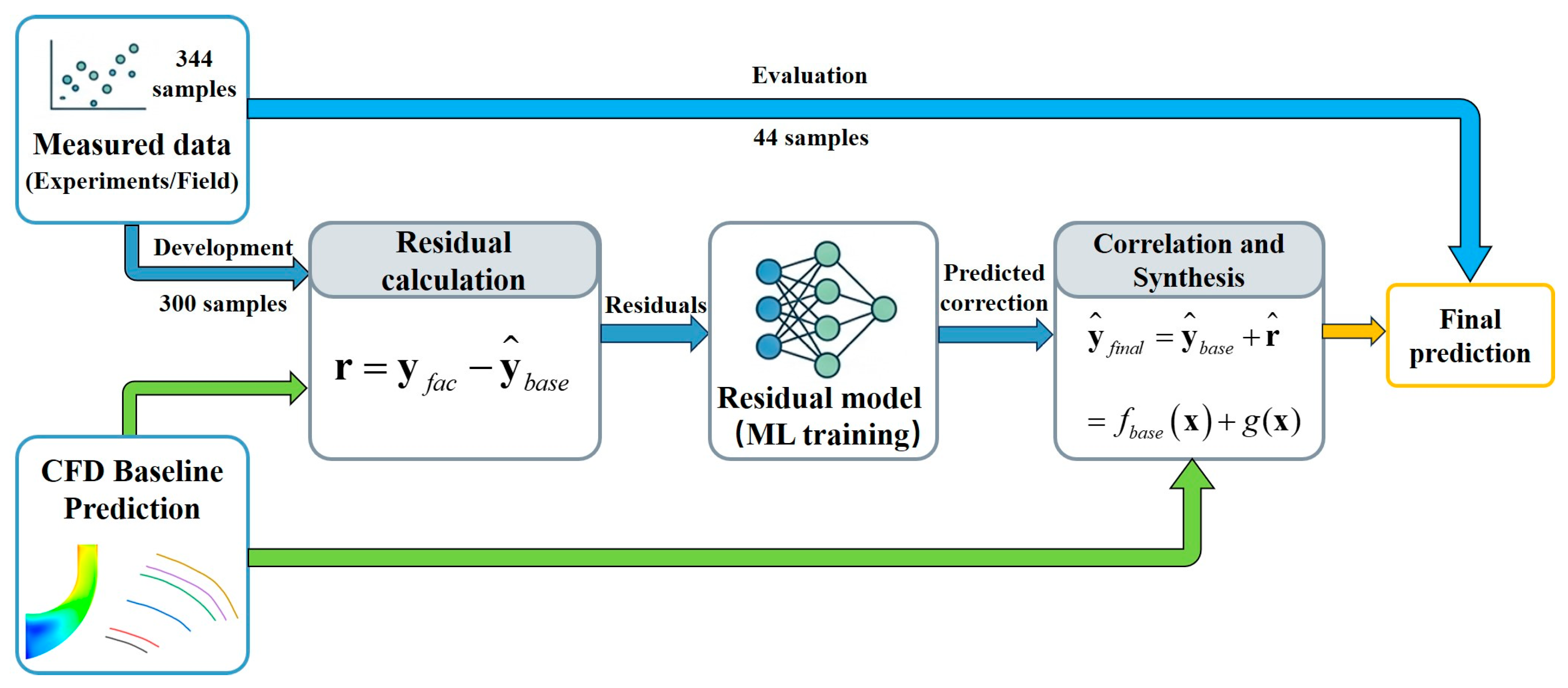Section 5 summarizes the main conclusions and future work. The overall workflow of the proposed method is illustrated in Figure 1. It includes reverse geometric reconstruction, full-machine CFD modeling and validation, multi-condition healthy-state sample generation, baseline model development, factory-data residual correction, and final validation using post-overhaul field data.

2. Numerical Simulation Method and Experimental Verification

2.1. Geometric Model, Mesh and Boundary Conditions

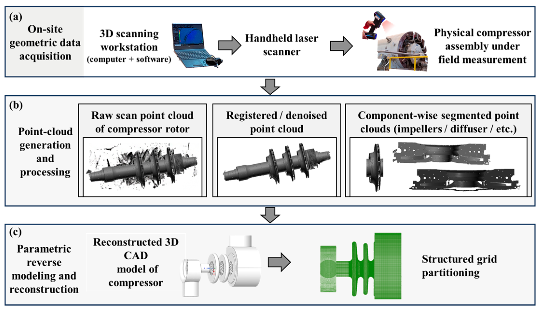
This study focuses on an in-use three-stage centrifugal compressor employed in a natural-gas compression station. As a widely used compressor type in China’s natural-gas transmission pipelines, it is selected here as an industrial case for developing and validating the proposed healthy-state modeling framework. To obtain a high-fidelity full-machine model, the geometry of the compressor flow passage was reconstructed by combining three-dimensional laser scanning and reverse modeling with the original factory structural parameters. A portable scanning device was used to acquire point-cloud data of the rotor, diffuser, return channel, and flow-guiding components. The scanned data were then fused and processed together with the original design parameters to generate a refined three-dimensional geometric model of the entire flow passage, followed by the creation of a structured grid, as illustrated in Figure 2.

Because the present work focuses on stable operating performance rather than transient instabilities, the compressor flow was treated as steady. The inlet boundary was specified as a pressure inlet with prescribed pressure and temperature, while the outlet boundary was specified as a mass-flow outlet. Since the transport capacity of the compressor varies with rotational speed, the mass flow rate was determined according to the actual operating condition, and the inlet volumetric flow rate was used as one of the principal external descriptors. The rotational speed was imposed on the impeller domains, while stationary components such as the diffuser, return channel, and casing were treated as fixed domains. The impeller rotation was handled through mesh motion, and the interface treatment was used for communication between rotating and stationary zones. Standard non-slip wall conditions were imposed, and a second-order upwind discretization scheme was adopted. A pressure-based coupled solver was used together with the energy equation to account for gas compressibility. The residual convergence criterion was set to 10⁻⁵, and key physical quantities such as outlet pressure, outlet temperature, and enthalpy change were monitored to ensure that the fluctuations remained within 1% and that the mass-conservation error also remained below 1%.

2.2. Turbulence Model, Real-Gas Equation of State, and Performance Definitions

The internal flow of a centrifugal compressor is turbulent and compressible. Therefore, the numerical model solves the Reynolds-averaged conservation equations of mass, momentum, and energy, together with an appropriate turbulence closure.

$${\displaystyle \frac{\partial \rho }{\partial t}}+{\displaystyle \frac{\partial (\rho v_j)}{\partial x_j}}=0$$

(1)

$${\displaystyle \frac{\partial (\rho v_i)}{\partial t}}+{\displaystyle \frac{\partial (\rho (v_i{v}_j))}{\partial x_j}}=-{\displaystyle \frac{\partial P}{\partial x_i}}+{\displaystyle \frac{\partial }{\partial x_j}}\left[\left(\mu +{\mu }_T\right)\left({\displaystyle \frac{\partial v_i}{\partial x_j}}+{\displaystyle \frac{\partial v_j}{\partial x_i}}\right)-{\displaystyle \frac{2}{3}}\rho \kappa \right]+S_{M,i}$$

(2)

$$\begin{array}{l}{\displaystyle \frac{\partial (\rho h_t)}{\partial t}}+{\displaystyle \frac{\partial (\rho h_t{v}_j)}{\partial x_j}}={\displaystyle \frac{\partial P}{\partial t}}+{\displaystyle \frac{\partial }{\partial x_j}}\left[k{\displaystyle \frac{\partial T}{\partial x_j}}+{\displaystyle \frac{{\mu }_T}{P{r}_T}}{\displaystyle \frac{\partial h}{\partial x_j}}\right]\\ +{\displaystyle \frac{\partial }{\partial x_j}}\left[v_i\left(\mu +{\mu }_T\right)\left({\displaystyle \frac{\partial v_i}{\partial x_j}}+{\displaystyle \frac{\partial v_j}{\partial x_i}}\right)-{\displaystyle \frac{2}{3}}{v}_j\rho \kappa \right]+S_E\end{array}$$

(3)

The SST k-ω turbulence model was selected because it combines the near-wall robustness of the k-ω formulation with the free-stream behavior of the k-ε model and is widely used for adverse-pressure-gradient and rotating-machinery flows [29]. The transport equations for turbulent kinetic energy and specific dissipation rate were adopted in their standard SST form.

$${\displaystyle \frac{\partial \rho k}{\partial t}}+{\displaystyle \frac{\partial \rho u_{j}k}{\partial x_j}}=P_k-{\beta }^{*}\rho \omega k+{\displaystyle \frac{\partial }{\partial x_j}}\left[\left(\mu +{\sigma }_k{\mu }_t\right)\cdot {\displaystyle \frac{\partial k}{\partial x_j}}\right]$$

(4)

$${\displaystyle \frac{\partial \rho \omega }{\partial t}}+{\displaystyle \frac{\partial \rho u_j\omega }{\partial x_j}}={\displaystyle \frac{\gamma \rho }{{\mu }_t}}\cdot P_k-\beta \rho {\omega }^2+{\displaystyle \frac{\partial }{\partial x_j}}\left[\left(\mu +{\sigma }_{\omega }{\mu }_t\right)\cdot {\displaystyle \frac{\partial \omega }{\partial x_j}}\right]+2\cdot (1-F_1){\displaystyle \frac{\rho {\sigma }_{\omega 2}}{\omega }}{\displaystyle \frac{\partial k}{\partial x_j}}{\displaystyle \frac{\partial \omega }{\partial x_j}}$$

(5)

To describe the thermodynamic properties of the transported natural gas, the Peng–Robinson equation of state was adopted in the CFD calculation [30]. The suitability of PR-EOS for the present methane-dominant natural-gas mixture was further evaluated by comparing it with GERG-2008 over the operating range of this study [31,32]. The comparison was conducted at inlet pressures of 6.5, 6.95, 7.1, 7.5, and 8.0 MPa and inlet temperatures of 20, 25, 30, and 35 °C using the gas composition listed in

Table 1. Comparison between PR-EOS and GERG-2008 for the natural-gas mixture.

CH4	N2	CO2	C2H6	C3H8	n-Butane	I-Butane	I-Pentane
92.54%	0.84%	1.89%	3.96%	0.34%	0.09%	0.12%	0.22%

. The evaluated thermodynamic properties included compressibility factor, density, specific enthalpy, and specific heat ratio. The maximum relative deviations between PR-EOS and GERG-2008 were 1.09% for compressibility factor, 1.11% for density, 1.35% for specific enthalpy, and 1.72% for specific heat ratio. These deviations are smaller than the CFD-model discrepancy observed against factory measurements and are therefore considered acceptable for constructing the CFD-generated baseline. The results of this EOS comparison are summarized in

Table 2. Comparison between PR-EOS and GERG-2008 for the natural gas.

Property	Maximum Relative Deviation	Average Relative Deviation	Operating Range
Compressibility factor	1.09%	0.95%	6.5–8.0 MPa, 20–35 °C
Density	1.11%	0.96%	6.5–8.0 MPa, 20–35 °C
Specific enthalpy	1.35%	0.88%	6.5–8.0 MPa, 20–35 °C
Specific heat ratio	1.72%	1.55%	6.5–8.0 MPa, 20–35 °C

.

The thermal performance of the compressor was evaluated using standard engineering indicators, including outlet pressure (p_out), outlet temperature (T_out), power (P_kW), polytropic head (H_Pol), and polytropic efficiency (η_pol). Outlet pressure and outlet temperature were directly taken from the simulated or measured thermodynamic states, whereas power, polytropic head, and polytropic efficiency were calculated from the corresponding inlet and outlet states, the inlet volumetric flow rate, and the real-gas thermodynamic relations adopted in this study. In this way, the predicted and measured performance indicators were defined on a consistent basis for validation and comparison. Accordingly, the calculated performance indicators, namely power, polytropic head, and polytropic efficiency, are defined as follows:

$$H_{pol}={\displaystyle {\displaystyle \underset{p_{in}}{\overset{p_{out}}{\int }}}vdp}$$

(6)

$$W_{tot}=h_{out}-h_{in}$$

(7)

$$P_{kW}=M\cdot W_{tot}$$

(8)

$${\eta }_{pol}={\displaystyle \frac{H_{pol}}{W_{tot}}}$$

(9)

For real-gas conditions, the polytropic head was not evaluated using a simple two-point approximation. Instead, the pressure path between the inlet and outlet states was discretized into N subintervals, and the integral of specific volume with respect to pressure was evaluated numerically. In the present calculation, the pressure was divided into 100 equally spaced intervals, and the gas state at each pressure level was obtained from the selected EOS along the polytropic path. The integral was evaluated using the composite Simpson quadrature scheme.

A sensitivity analysis was performed using N = 20, 50, 100, 200 integration intervals. The resulting variation in polytropic head was 0% when N exceeded 100, indicating numerical convergence of the thermodynamic integral. The sensitivity results are reported in

Table 3. Sensitivity of real-gas polytropic-head integration to quadrature resolution.

Number of Integration Intervals	Polytropic Head	Relative Change Compared with Finest Resolution
20	45.29	2.28%
50	44.58	0.68%
100	44.28	0
200	44.28	0

.

The power calculated from the CFD thermodynamic states corresponds to the aerodynamic or fluid power transferred to the gas, rather than the total mechanical shaft power including bearing friction, seal losses, disk friction, and other mechanical losses. To avoid ambiguity, the symbol P_kW in this paper is redefined as fluid power unless otherwise specified. When comparisons with factory shaft-power measurements are made, the residual-correction model implicitly accounts for the systematic difference between CFD-derived fluid power and factory-measured shaft power. This distinction is important because the CFD model alone does not explicitly resolve all mechanical-loss mechanisms.

To quantitatively evaluate the prediction accuracy of the model, relative errors were used for outlet pressure, power, polytropic head, and polytropic efficiency. For a generic variable y, the relative error is defined as

$${\delta }_y={\displaystyle \frac{\left|y_{pred}-y_{meas}\right|}{y_{meas}}}\times 100\%$$

(10)

Since the outlet temperature is strongly influenced by the inlet thermal condition, its error was evaluated using the temperature rise across the compressor, rather than the absolute outlet temperature itself. The corresponding relative error is defined as

$$\mathrm{\Delta }T=T_{out}-T_{in}$$

(11)

$${\delta }_{\mathrm{\Delta }T}={\displaystyle \frac{\left|\mathrm{\Delta }{T}_{pred}-\mathrm{\Delta }{T}_{meas}\right|}{\mathrm{\Delta }{T}_{meas}}}\times 100\%$$

(12)

In addition, the average relative error and the maximum relative error over all samples were used to assess the overall model accuracy.

2.3. Grid Independence Verification and Experimental Verification

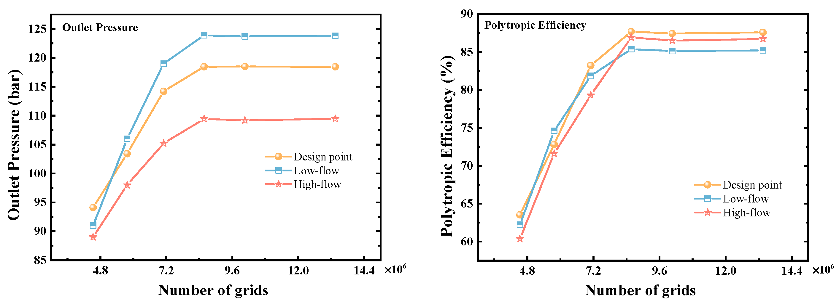
Grid independence is essential for ensuring that the numerical predictions are not materially affected by mesh resolution under three operating conditions: low flow, design flow, and high flow. Six groups of structured meshes, ranging from 4.533 million to 13.353 million cells, were generated and evaluated under three operating conditions: low-flow, design-flow, and high-flow conditions. The inlet pressure, inlet temperature, and rotational speed were kept constant at 6.5 MPa, 25 °C, and 5910 r/min, respectively. The flow rates for the low-flow, design-flow, and high-flow conditions were set to 12,000, 15,000, and 18,000 m³/h, respectively. The grid-independence results are presented in Figure 3. The results showed that when the number of grid cells was below 8.575 million, outlet pressure and polytropic efficiency changed noticeably with mesh refinement, whereas the results became stable once the mesh size reached 8.575 million cells. Therefore, the mesh with 8.575 million cells was selected for all subsequent calculations.

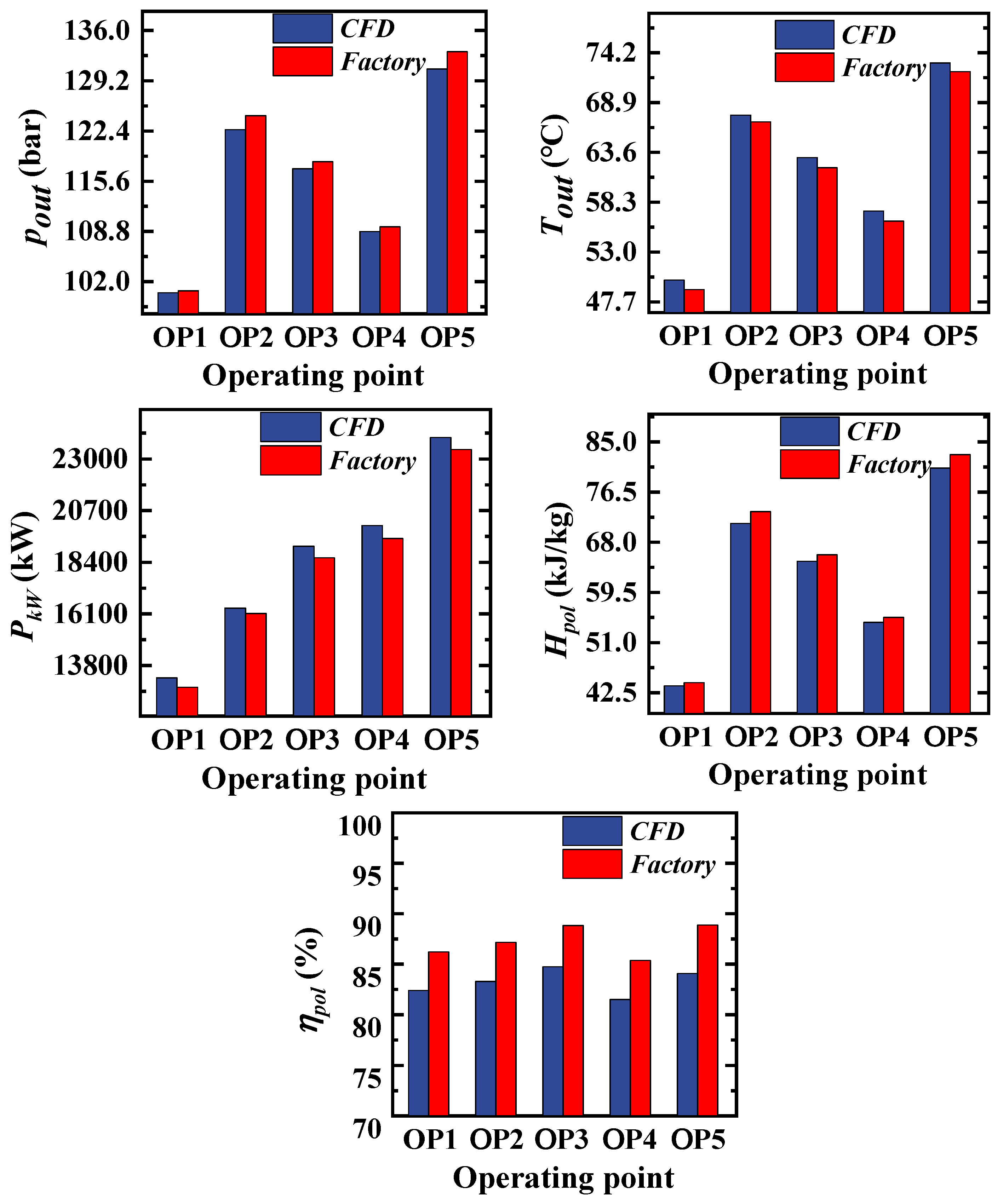
To verify the reliability of the CFD model, the study compared the CFD predictions with factory measurements at five representative operating points. The selected points were designed to cover two key validation dimensions: rotational-speed variation at the design-flow condition and flow-rate variation at the design-speed condition. In particular, OP1, OP3, and OP5 represent the design-flow condition at low, design, and high rotational speeds, respectively, whereas OP2, OP3, and OP4 represent the low-flow, design-flow, and high-flow conditions at the design rotational speed. This configuration allows the CFD model to be validated from both the speed and flow-rate perspectives.

As shown in Figure 4, the CFD predictions agree well with the factory data in terms of outlet pressure, outlet temperature, power, polytropic head, and polytropic efficiency over representative operating points. The maximum relative errors of the simulated outlet pressure, temperature rise, power, polytropic head, and polytropic efficiency were 1.779%, 3.496%, 3.202%, 2.724%, and 5.381%, respectively. The average relative errors of the simulated outlet pressure, temperature rise, power, polytropic head, and polytropic efficiency were 0.994%, 2.446%, 2.523%, 1.973%, and 4.676%, respectively. These errors are within an acceptable engineering range, and the variation trends of the simulated quantities are consistent with the measured factory data. Therefore, the validated CFD model can provide a reliable basis for the construction of the healthy-state baseline.

The five operating points used for CFD validation were obtained from the manufacturer/factory performance-test report of the investigated compressor under healthy-state conditions. These points were selected because they cover both rotational-speed variation and flow-rate variation around the design operating condition. Specifically, OP1, OP3, and OP5 represent different rotational speeds at or near the design-flow condition, whereas OP2, OP3, and OP4 represent different flow-rate conditions at or near the design rotational speed. Therefore, the five points provide representative validation evidence along the two most important operating dimensions of the compressor map.

The measured quantities used for validation include inlet pressure, inlet temperature, outlet pressure, outlet temperature, rotational speed, flow rate, and power. The accuracy of the corresponding instruments is summarized in

Table 4. Factory-data instrumentation and measurement uncertainty.

Variable	Instrument/Signal Source	Accuracy or Uncertainty
Inlet pressure	Inlet pressure transmitter	±0.075–0.10% FS
Outlet pressure	Outlet pressure transmitter	±0.075–0.10% FS
Inlet temperature	Pt100 RTD or thermocouple	±0.2–0.5 K
Outlet temperature	Pt100 RTD or thermocouple	±0.2–0.5 K
Flow rate	Station flowmeter	±0.5–1.5% of reading
Rotational speed	Tachometer, encoder, or control-system signal	±0.01–0.05% of reading or ±1 r/min
Shaft/fluid power	Power meter, torque meter, or calculated fluid power	±0.5–1.0% for shaft power; propagated uncertainty for fluid power
Gas composition	Gas chromatograph	±0.01–0.05 mol% for major components

. The uncertainty of derived quantities, including fluid power, polytropic head, and polytropic efficiency, was evaluated by uncertainty propagation. Although the number of direct factory validation points is limited, these points cover both speed and flow-rate variation and are therefore suitable for validating the major trend of the full-machine CFD model before generating the multi-condition CFD database.

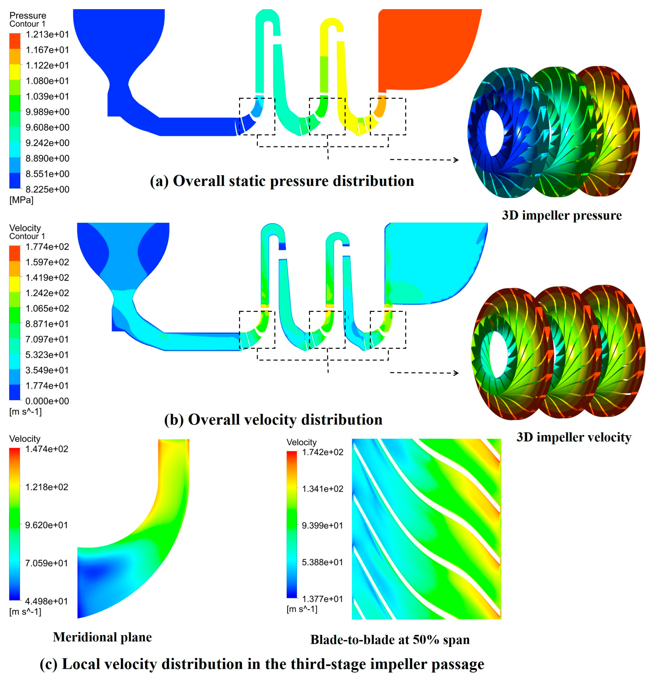
Besides the quantitative comparison with factory measurements, the physical rationality of the CFD model was further examined through typical flow-field distributions, as shown in Figure 5. Figure 5a shows the overall static-pressure distribution of the three-stage compressor, where a clear stage-by-stage pressure rise can be observed along the flow path. Figure 5b presents the velocity distribution on the meridional mid-span section, revealing the expected periodic acceleration and deceleration of the flow through the impeller, diffuser, and return-channel passages. Figure 5c presents the local velocity distribution in a representative impeller, including the meridional plane and the blade-to-blade plane at 50% span, indicating a physically reasonable flow development within the blade passage. These results further support the physical credibility of the CFD-generated healthy-state baseline model.

3. Construction of the Healthy-State Performance Model

3.1. Construction of the CFD-Generated Healthy-State Database

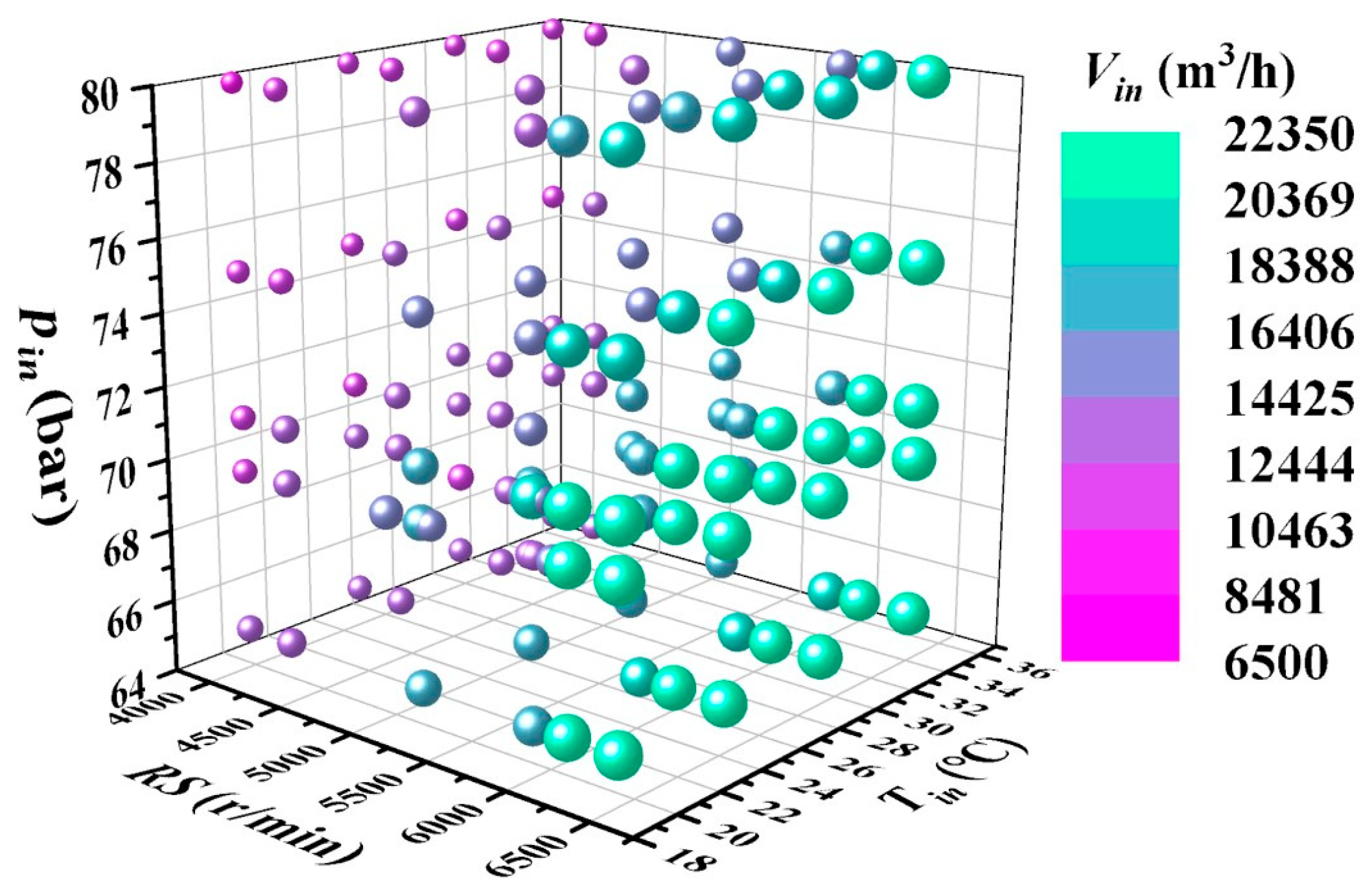
Based on the validated numerical model, a full-condition CFD sample library was established to support the construction of the healthy-state baseline. The design operating condition of the target compressor corresponds to a rotational speed of 5889 r/min, an inlet pressure of 7.1 MPa, an inlet temperature of 20 °C, and a flow rate of 15,000 m³/h. Around this design point, a full-factor operating-condition matrix was constructed. The inlet pressure was set to 6.5, 6.95, 7.1, 7.5, and 8.0 MPa; the inlet temperature was set to 20, 25, 30, and 35 °C; the rotational speed was set to 3965, 4270, 5185, 5889, 6100, and 6405 r/min; and, for each rotational speed, 12 uniformly spaced inlet volumetric flow-rate levels were defined according to the allowable operating range. This procedure yielded a total of 1440 operating points. To improve computational efficiency, a 256-core CPU platform was used for parallel simulations and batch sample generation. The total wall-clock time required to generate the complete CFD database was approximately 480 h, corresponding to an average wall-clock time of approximately 20 min per operating point under the adopted parallel-computing arrangement.

Figure 6 shows the spatial distribution of 1440 CFD simulation points. The three axes correspond to rotational speed, inlet temperature, and inlet pressure, while the inlet volumetric flow rate is mapped through a color scale. This point cloud indicates that the CFD cases were generated by conducting structured sampling in the multi-dimensional operating space, which helps to verify that this database covers a wide range of target operating conditions. The ranges of inlet pressure, inlet temperature, rotational speed, and inlet volumetric flow rate were determined according to the design condition, factory performance curve, and actual allowable operating envelope of the compressor. The structured sampling strategy covers both the design condition and typical off-design states, including low-speed, high-speed, low-flow, and high-flow conditions. Therefore, the CFD database is not limited to a narrow neighborhood around the design point but covers the main operating region required for healthy-state baseline construction.

3.2. Factory-Data Quality and Uncertainty Characterization

A total of 344 sets of factory test data were used in this study. To ensure data quality, the raw measurements were screened according to thermodynamic steady-state criteria before being used for model correction and validation. A sample was regarded as quasi-steady only when the variations in inlet pressure, inlet temperature, rotational speed, and inlet volumetric flow rate within a 5 min window were lower than 0.3%, 0.5 K, 0.2%, and 1%, respectively. Samples failing these criteria were excluded from the factory-data correction dataset.

The main measurement instruments and their accuracies are listed in Table 4. The uncertainties of derived quantities, including polytropic head, efficiency, and power, were calculated using the law of propagation of uncertainty [33]. All instruments were calibrated according to traceable calibration procedures or manufacturer-recommended methods. The uncertainty of calculated fluid power was obtained by propagating the uncertainties of flow rate, pressure, temperature, and gas composition.

For clarity, the CFD-generated database was used to train the healthy-state baseline surrogate. The factory correction dataset was used only to train the residual-correction model. Dataset A was held out from all training and hyperparameter-selection procedures and was used only for independent evaluation and ablation comparison. The post-overhaul field dataset was used as an additional quasi-steady field validation dataset.

3.3. Baseline-Model Development and Comparison of Algorithms

Before model development, all input features were standardized using StandardScaler. The CFD sample set was divided into training, validation, and test subsets in a ratio of 70:15:15. The training subset was used for model fitting, the validation subset was used for hyperparameter selection, and the independent test subset was used for final baseline-surface evaluation. The factory data were divided into 300 samples for residual-correction training and 44 independent samples for validation.

Four candidate algorithms, namely XGBoost, LightGBM, Random Forest, and MLP, were first compared using the same training, validation, and test split. The tree-based models were implemented with commonly used fixed hyperparameter settings to provide a reproducible baseline comparison. Since MLP showed the best overall performance in the candidate-model comparison, it was further adopted for the CFD baseline surrogate, the factory-data-only model, and the residual-correction model. For the final MLP-based models, GridSearchCV with three-fold cross-validation was used to select the hidden-layer structure and L2 regularization coefficient. Four parameter combinations were evaluated for each output variable, corresponding to 12 model fits per output. The detailed model settings are summarized in

Table 5. Hyperparameter search space and final hyperparameters of the candidate models.

Model	Search Strategy	Search Budget	Main Search Space/Hyperparameters	Final Hyperparameters
XGBoost	Fixed-parameter setting for candidate-model comparison	1 configuration	n_estimators, max_depth, learning_rate, subsample, colsample_bytree	n_estimators = 800; max_depth = 7; learning_rate = 0.05; subsample = 0.8; colsample_bytree = 0.8; objective = reg:squarederror; tree_method = hist; random_state = 42
LightGBM	Fixed-parameter setting for candidate-model comparison	1 configuration	n_estimators, learning_rate, subsample, colsample_bytree	n_estimators = 800; learning_rate = 0.05; subsample = 0.8; colsample_bytree = 0.8; random_state = 42
Random Forest	Fixed-parameter setting for candidate-model comparison	1 configuration	n_estimators, max_depth	n_estimators = 300; max_depth = 10; random_state = 42
MLP	GridSearchCV with 3-fold cross-validation for final model construction	4 parameter combinations; 12 fits per output	hidden_layer_sizes, activation, learning_rate_init, alpha	hidden_layer_sizes = (64, 32) or (128, 64); activation = relu; solver = adam; learning_rate_init = 0.001; alpha = 1 × 10−4 or 1 × 10−3; max_iter = 800; early_stopping = True; validation_fraction = 0.15; n_iter_no_change = 20; tol = 1 × 10−4; random_state = 42

.

The final multilayer perceptron (MLP) contained two hidden layers, with either 64 and 32 neurons or 128 and 64 neurons selected by GridSearchCV for each output variable. The activation function was ReLU, the optimizer was Adam [34], the initial learning rate was 0.001, and the batch size was automatically determined by the scikit-learn MLPRegressor default setting. Early stopping was applied with a patience of 20 epochs, and L2 regularization coefficients of 1 × 10⁻⁴ and 1 × 10⁻³ were tested to reduce overfitting. The model was trained for a maximum of 800 epochs, and the weights corresponding to the lowest validation loss were retained. The MLP training procedure follows standard deep-learning practice [35].

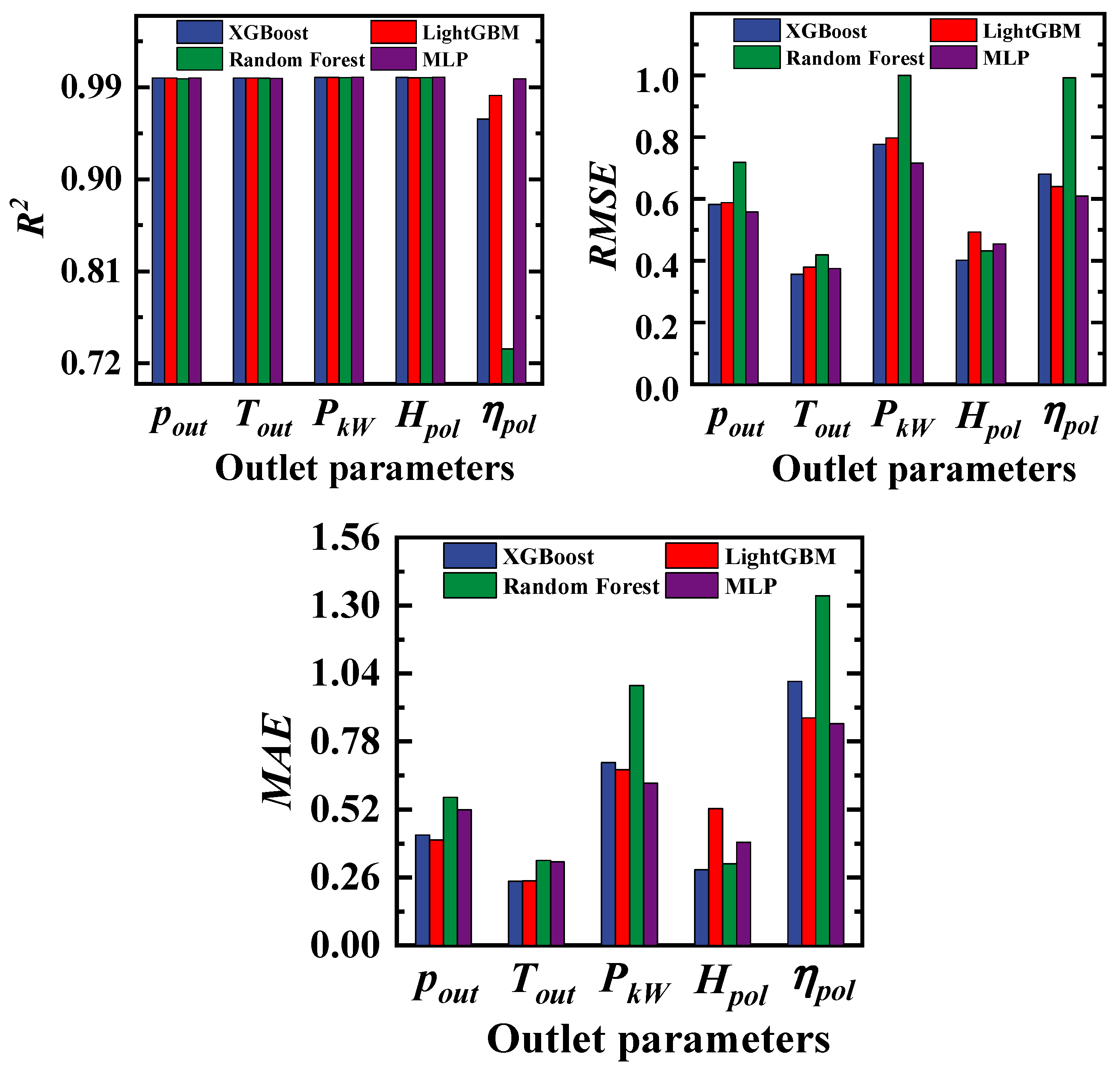
Figure 7 compares the predictive performance of the four candidate models in terms of R², RMSE, and MAE for the five output variables. The results show that all four models achieve high prediction accuracy for outlet pressure, outlet temperature, power, and polytropic head, with R² values exceeding 0.990. However, their behavior differs substantially for polytropic-efficiency prediction. In that case, Random Forest performs the worst, whereas MLP achieves the best accuracy, with R² = 0.99812. The RMSE and MAE comparison shows that MLP achieves the lowest or among the lowest RMSE and MAE values across most output variables, indicating better overall accuracy and robustness. Overall, MLP exhibits the best combined accuracy and robustness among the four candidate models.

3.4. Data Partition, Model Formulation, and Correction Strategy

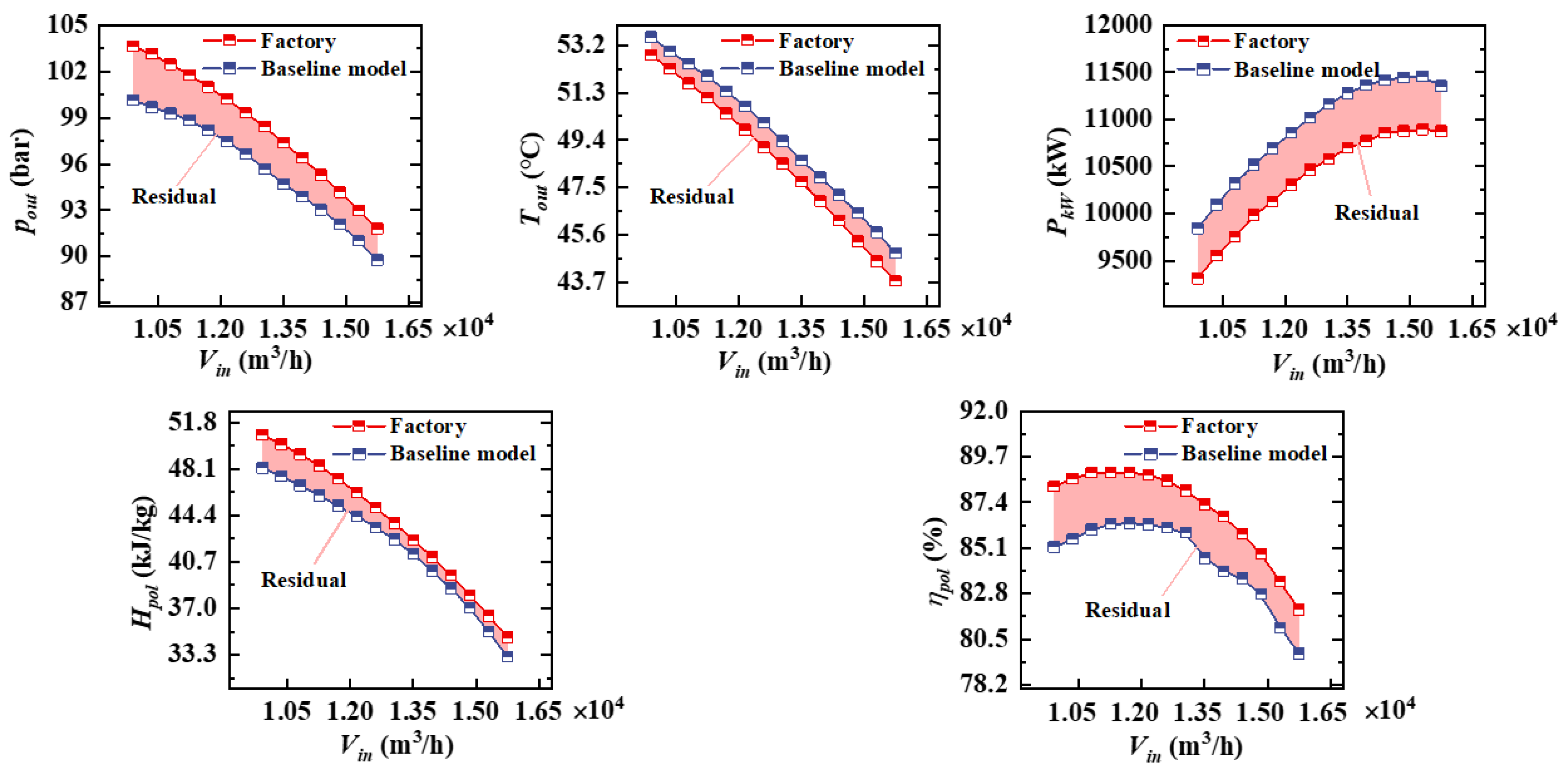
To assess whether the selected baseline model can be directly applied to the real machine, it was further compared with the measured factory data. As shown in Figure 8, although the baseline model reproduces the overall variation trends of outlet pressure, outlet temperature, power, polytropic head, and polytropic efficiency, noticeable discrepancies remain between the baseline predictions and the actual factory measurements. This indicates that, while the baseline model preserves the physically meaningful response derived from the validated CFD database, it cannot fully eliminate the systematic deviation between the numerical model and the real machine. Therefore, an additional residual-correction stage is required to improve engineering fidelity.

To support both independent comparison and residual correction, the measured factory data were further partitioned according to different purposes. A total of 344 sets of factory test data were collected under real-machine conditions. Among them, 44 sets were separated as an independent comparison subset, denoted as Dataset A, and were used to evaluate the engineering consistency of the selected baseline model against measured machine data. The remaining factory samples were used for the development of the residual-correction model.

To avoid potential data leakage, Dataset A was not used in baseline-model training, residual-correction fitting, hyperparameter selection, feature scaling, or early stopping. All preprocessing parameters used by the learning models were fitted only on the corresponding training data and then applied to Dataset A. Therefore, Dataset A served as a strictly independent evaluation subset. The operating-condition distribution of Dataset A lies within the envelope covered by the CFD database and overlaps with the factory correction dataset, so the evaluation reflects interpolation performance within the intended application domain rather than uncontrolled extrapolation.

For clarity, the overall data flow and correction mechanism of the proposed model are illustrated in Figure 9. As shown in Figure 9, the proposed framework consists of two coupled layers: a CFD-generated baseline model and a factory-data-driven residual-correction model. The baseline model provides the physically grounded healthy-state response under multiple operating conditions, whereas the correction model learns the systematic discrepancy between the baseline prediction and the real-machine performance.

The input vector is defined as

$$x={\left[p_{in},T_{in},n,V_{in}\right]}^{\mathrm{T}}$$

(13)

where p_in, T_in, n and Q_in denote inlet pressure, inlet temperature, rotational speed, and inlet volumetric flow rate, respectively. The output vector is written as

$$y={\left[p_{out},T_{out},P_{kW},H_{pol},{\eta }_{pol}\right]}^{\mathrm{T}}$$

(14)

where p_out, T_out, P_kW, H_pol and η_pol represent outlet pressure, outlet temperature, fluid power, polytropic head, and polytropic efficiency, respectively.

Based on the CFD dataset, the healthy-state baseline model can be expressed as

$${\widehat{y}}_{base}=f_{base}\left(x\right)$$

(15)

where f_base denotes the machine learning mapping learned from the validated CFD-generated healthy-state database. In the present study, several candidate algorithms were compared, and the multilayer perceptron (MLP) was finally selected as the baseline model.

Although the CFD-generated baseline preserves the physical response of the compressor under multiple operating conditions, a systematic discrepancy may still exist between the CFD-based prediction and the actual machine performance. To characterize this discrepancy, the residual vector is defined as

$$r=y_{fac}-{\widehat{y}}_{base}$$

(16)

where y_fac is the corresponding measured factory output vector. Since the correction stage is intended to compensate for systematic deviation under the same operating-condition descriptors, the residual model uses the same input vector x as the baseline model. It can therefore be written as

$$\widehat{r}=g(x)$$

(17)

where g denotes the residual-correction model trained using the measured factory data.

Accordingly, the final corrected healthy-state model is expressed as

$${\widehat{y}}_{final}={\widehat{y}}_{base}+\widehat{r}=f_{base}\left(x\right)+g(x)$$

(18)

This formulation shows that the proposed model is composed of two coupled layers: a CFD-generated healthy-state baseline that provides the physically grounded response of the compressor, and a factory-data-driven residual correction that improves engineering fidelity. Therefore, the final model retains the physical consistency of the CFD baseline while achieving better agreement with the actual machine performance.

3.5. Factory-Data Correction of the CFD-Generated Baseline

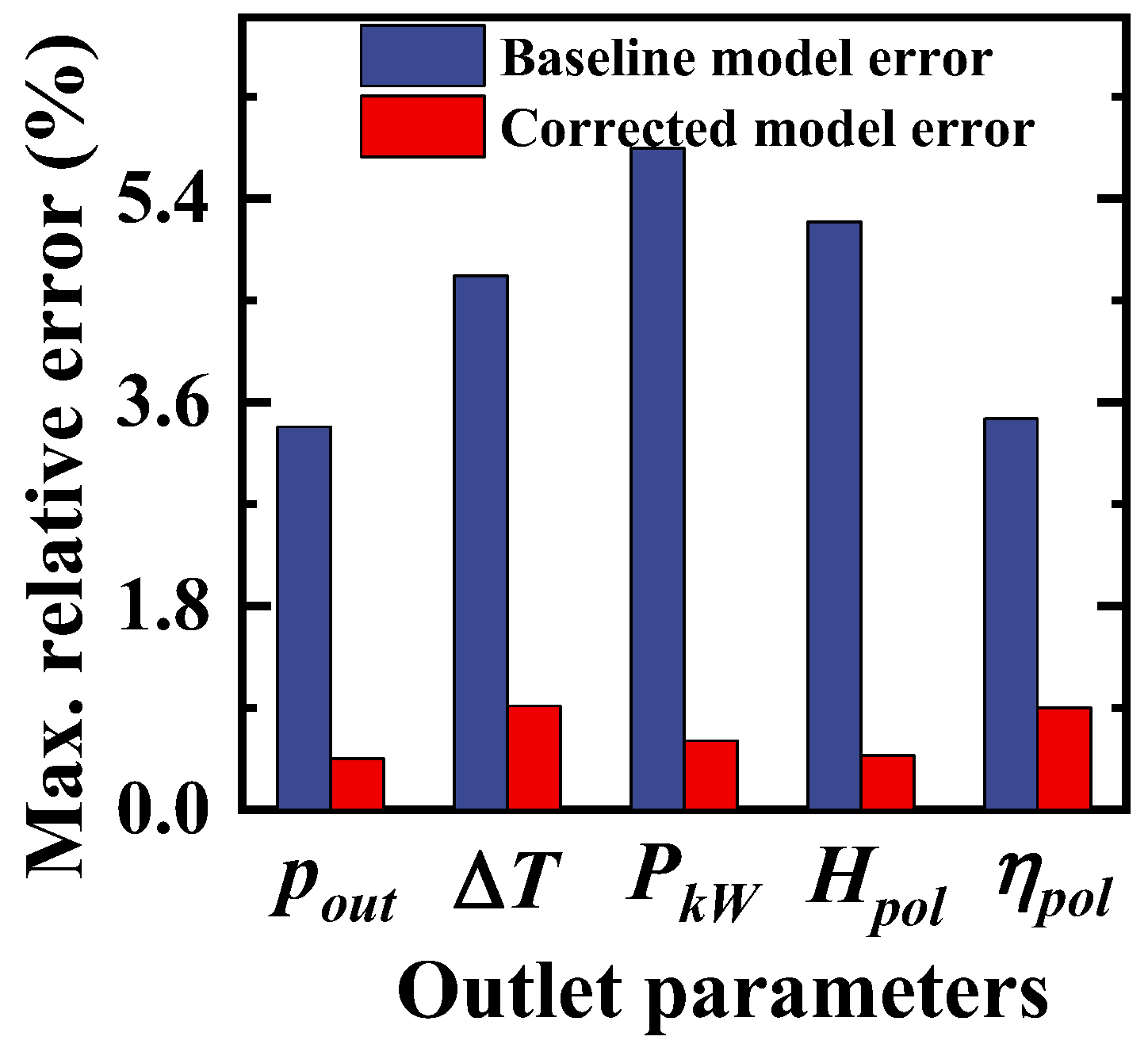
To quantitatively evaluate the improvement achieved by the residual correction, Figure 10 presents a comparison of the maximum relative errors of the major performance indicators before and after correction (data from Dataset A). The figure shows that after residual correction, the maximum relative errors of all major performance indicators are significantly reduced. Specifically, the maximum relative errors of outlet pressure, temperature rise, power, polytropic head, and polytropic efficiency decrease to 0.451%, 0.918%, 0.611%, 0.481%, and 0.899%, respectively.

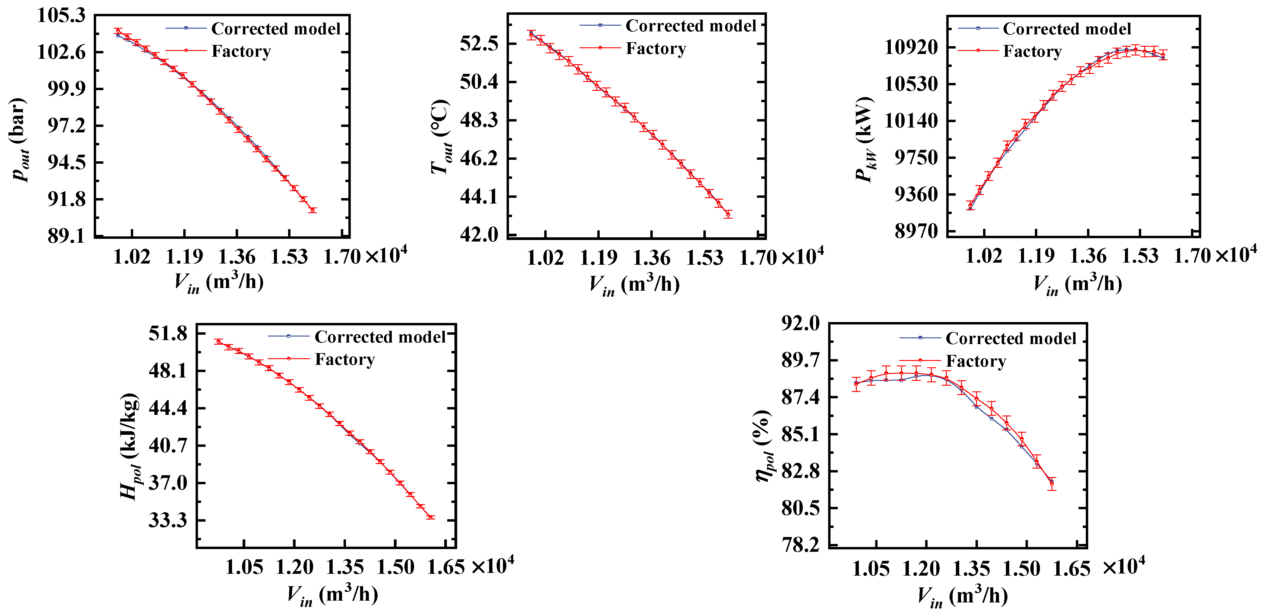
Figure 11 compares the final corrected model with the operating conditions of Dataset A. It can be observed that the final model achieves higher prediction accuracy and better agreement with Dataset A than the original CFD-based baseline model.

These results indicate that the corrected model not only preserves the physically meaningful trends embodied in the CFD-generated baseline, but also achieves substantially better agreement with the actual factory performance curve.

Overall, the factory-data-driven residual correction plays a crucial role in bridging the gap between the validated CFD baseline and the real machine. Therefore, the final corrected model combines the physical interpretability of the CFD-generated healthy-state baseline with the engineering accuracy required for practical condition assessment and performance evaluation.

3.6. Ablation Study of the CFD Baseline, Factory-Data-Only Model, and Proposed Hybrid Model

To clarify the contribution of each modeling component, an ablation study was conducted. Three models were compared using the same independent factory validation subset, Dataset A: (a) the CFD-generated baseline surrogate without factory-data correction, (b) a factory-data-only model trained using the same 300 factory samples used for residual correction, and (c) the proposed hybrid model combining the CFD-generated baseline and factory-data residual correction. The factory-data-only model used the same input variables and the same candidate algorithm family as the proposed correction model, and its hyperparameters were tuned under the same search budget.

The results are summarized in

Table 6. Ablation comparison on Dataset A.

Model	Outlet Pressure Max/Avg Error	Temperature-Rise Max/Avg Error	Power Max/Avg Error	Polytropic Head Max/Avg Error	Polytropic Efficiency Max/Avg Error
CFD baseline	5.156%/1.217%	8.348%/1.212%	7.292%/1.290%	14.765%/2.638%	9.802%/1.482%
Factory-data-only model, 300 samples	1.651%/0.346%	5.512%/0.909%	11.786%/1.024%	5.725%/0.564%	1.111%/0.219%
Proposed hybrid model	0.451%/0.167%	0.918%/0.403%	0.611%/0.510%	0.481%/0.362%	0.899%/0.143%

. The CFD baseline preserves physically reasonable performance trends but shows systematic deviations from the real machine. The factory-data-only model benefits from direct measurement data but is limited by the small sample size and weaker extrapolation robustness. The proposed hybrid model achieves the lowest overall validation error, indicating that the CFD baseline and factory-data correction provide complementary information.

3.7. SHAP-Based Interpretability Analysis

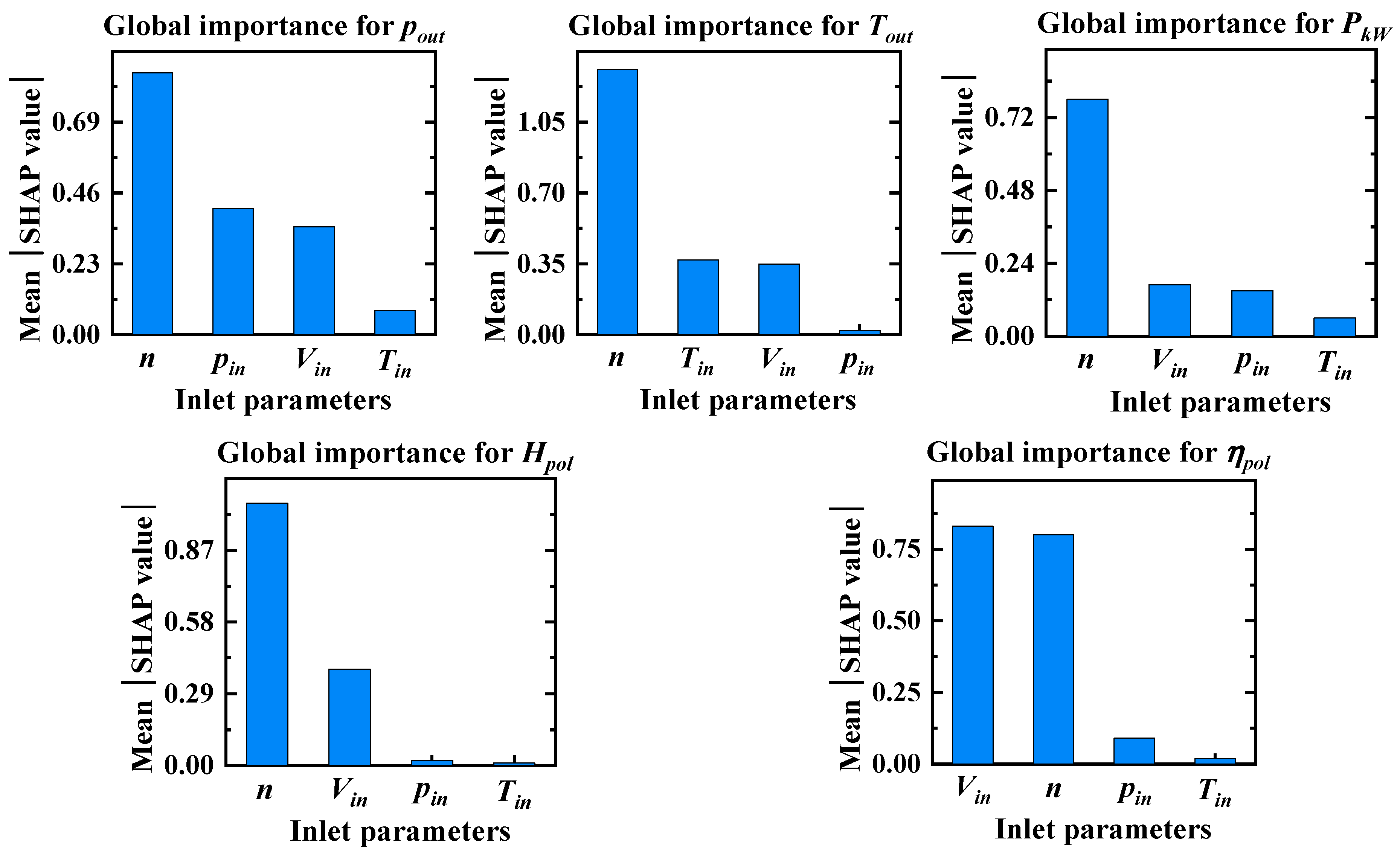
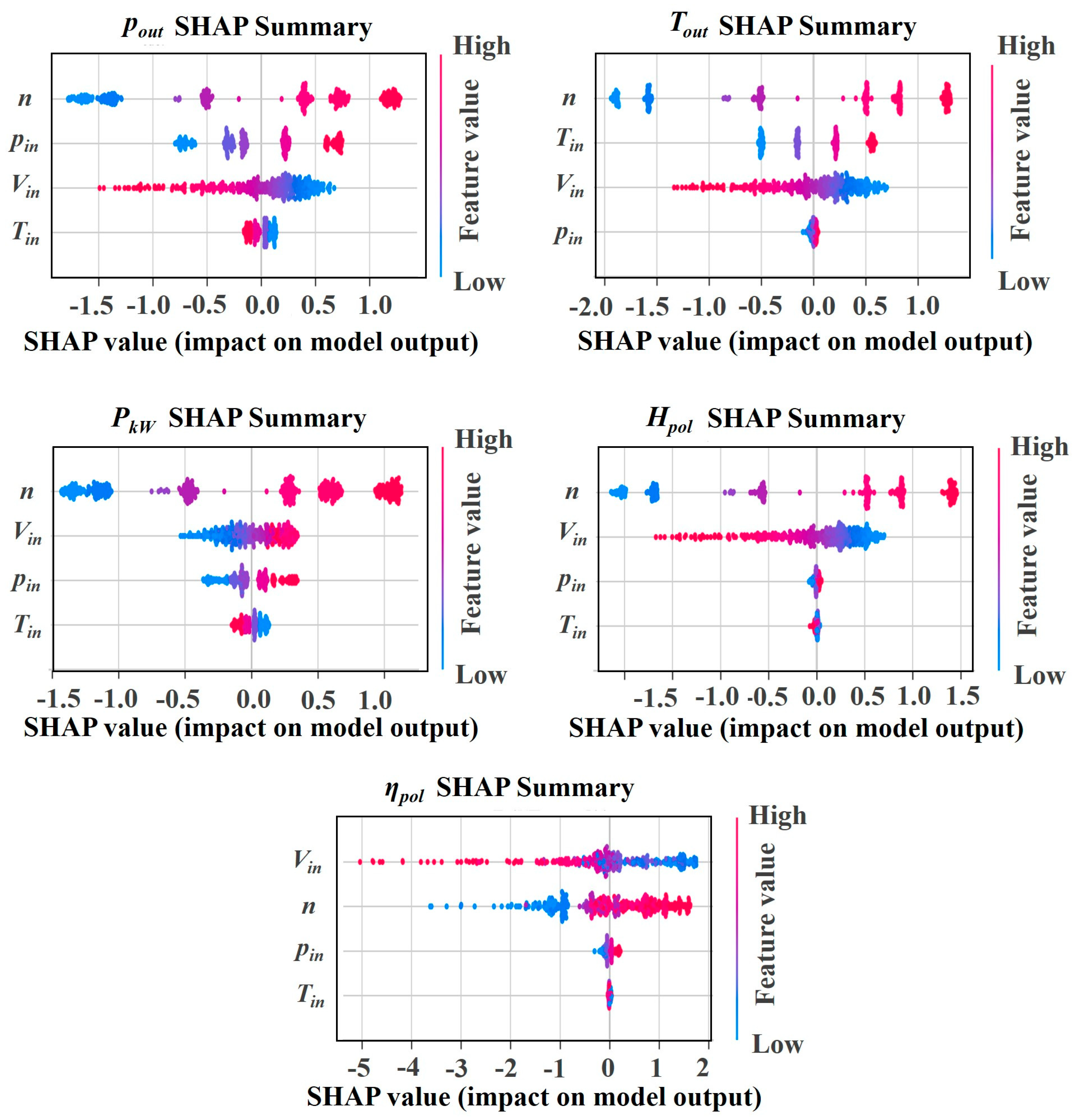
To improve the interpretability of the final model, SHAP analysis was performed for the major output variables. As shown in Figure 12, the results show that rotational speed is the dominant factor for outlet pressure, temperature, power, and polytropic head, whereas inlet volumetric flow rate plays the leading role in polytropic-efficiency prediction. Inlet pressure has moderate importance, while inlet temperature is generally less influential except in temperature-related prediction. Overall, the feature-importance ranking is consistent with compressor operating physics.

The SHAP summary plots further reveal the contribution direction of each input. As shown in Figure 13, rotational speed contributes positively to pressure, temperature rise, power, and head. Inlet volumetric flow rate generally has a negative effect on pressure, head, and efficiency under high-flow conditions, while its influence on power is nonlinear. Inlet pressure mainly enhances outlet pressure and power, whereas inlet temperature primarily increases temperature rise and shows only a weak effect on the other outputs. These results confirm that the final model is physically interpretable rather than a purely black-box predictor.

The SHAP results are also consistent with the physical similarity relationships of centrifugal compressors. Rotational speed directly determines the impeller tip speed and therefore controls the specific work transferred from the impeller to the gas. As the pressure rise and polytropic head are closely related to the square of the tip speed, changes in rotational speed naturally produce dominant contributions to outlet pressure and polytropic head. The temperature rise and fluid power are also strongly associated with the energy input to the gas, which explains why rotational speed has the largest SHAP contribution for outlet temperature and power.

In contrast, polytropic efficiency is more sensitive to the inlet volumetric flow rate because the flow rate determines the position of the operating point relative to the best-efficiency region. When the flow rate deviates from the optimal range, incidence losses, diffusion losses, separation losses, secondary-flow losses, and leakage-related losses may increase. Therefore, inlet volumetric flow rate becomes the dominant variable for polytropic-efficiency prediction. This result indicates that efficiency degradation should not be diagnosed only from a decrease in efficiency itself, but should be interpreted together with the operating flow condition.

From a monitoring and diagnostic perspective, the SHAP results suggest that deviations in pressure, temperature rise, power, and head should first be normalized with respect to rotational-speed changes, whereas deviations in efficiency should be evaluated together with the flow-rate operating region. This helps distinguish true health-related degradation from normal off-design operation. The feature-importance results therefore provide not only model interpretability, but also practical guidance for defining condition-monitoring thresholds and selecting diagnostic indicators.

3.8. Inference Latency and Real-Time Deployment

The real-time capability of the proposed framework refers to the online inference stage only. The CFD simulations, database generation, and model training are performed offline. During online deployment, the SCADA system provides inlet pressure, inlet temperature, rotational speed, and inlet volumetric flow rate as model inputs. The trained baseline surrogate and residual-correction model then output the corresponding healthy-state performance indicators.

To evaluate deployment feasibility, the inference latency of the final model was benchmarked on Intel64 Family 6 Model 183 Stepping 1, GenuineIntel, running Windows-10-10.0.22631-SP0 with Python 3.10.11. After 100 warm-up runs, the average inference time for a single sample was 0.6584 ms, and the 95th percentile latency was 0.8891 ms over 3000 repeated runs. The median latency was 0.6176 ms, and the maximum latency was 3.2946 ms. Since the SCADA sampling interval of the compressor station is 60 s, the online inference time is much shorter than the data acquisition cycle. Therefore, the trained model is computationally compatible with real-time condition assessment.

4. Validation Using Post-Overhaul Field Data

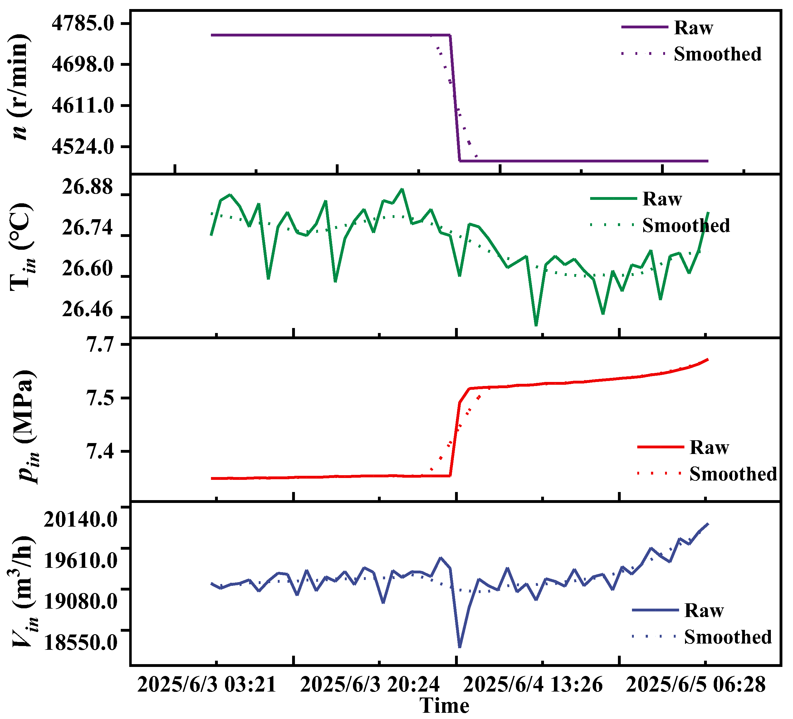
The post-overhaul field dataset was used to evaluate the applicability of the final model under practical station conditions. Because the model was developed under steady-state assumptions, the field data were divided into quasi-steady operating segments and rapid transition periods. The quasi-steady samples were identified using the same stability criteria as those applied to the factory data. Samples during rapid speed adjustment were retained only for trend visualization and were not used for the main quantitative error statistics unless explicitly stated. The time-series profiles of the selected post-overhaul field data are shown in Figure 14, where the variations in rotational speed and operating conditions before and after speed adjustment can be clearly observed.

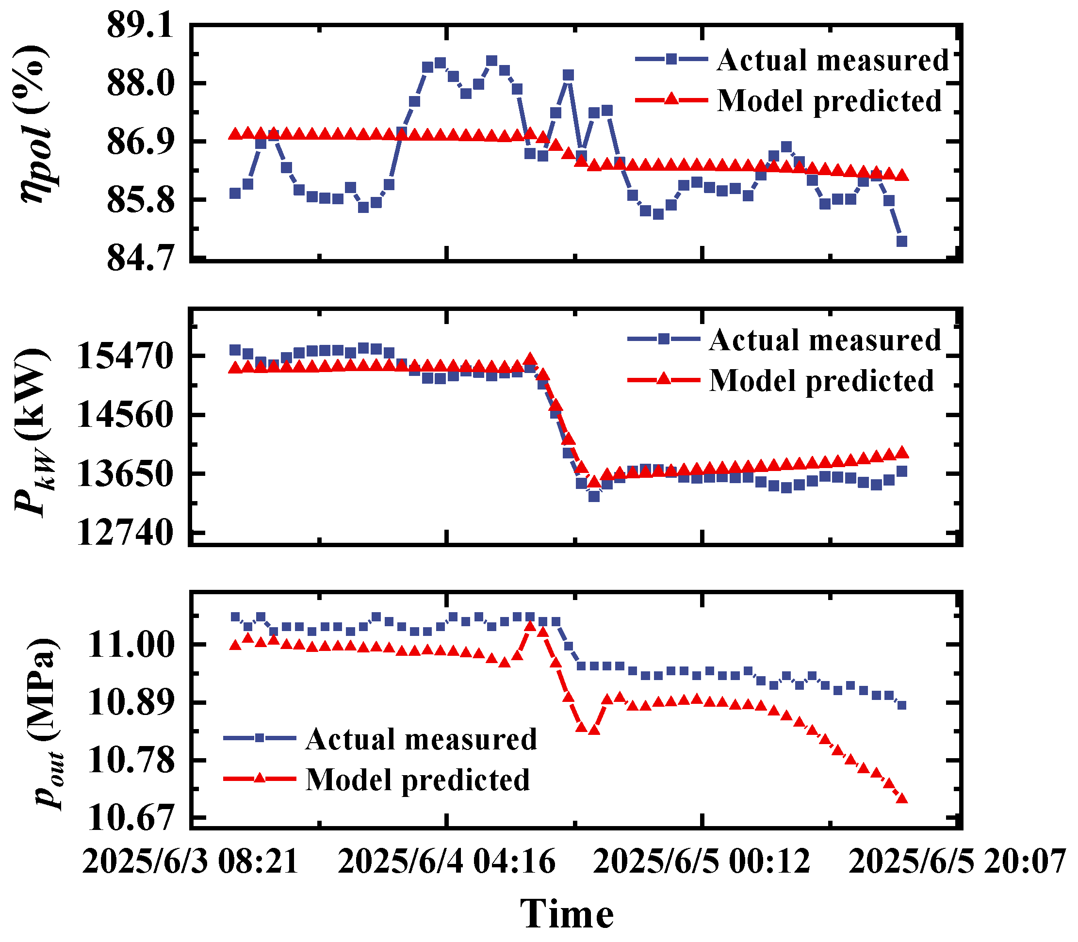
The comparison between the model predictions and the measured data in Figure 15 shows that the predicted trends are highly consistent with the actual operating behavior of the machine. The average relative errors of outlet pressure, power, and polytropic efficiency are 0.626%, 1.228%, and 0.807%, respectively. The maximum relative errors of outlet pressure, power, and polytropic efficiency are 1.650%, 3.048%, and 1.708%, respectively. The post-overhaul errors are larger than those obtained on the factory validation subset. This difference may be attributed to multiple factors, including post-overhaul assembly and clearance deviations, measurement noise, sensor drift, differences between factory and field gas compositions, residual transient effects during speed changes, and differences between factory test conditions and station operation.

From an engineering perspective, the 3.048% maximum power error indicates that the corrected healthy-state model should not be used to diagnose very small power deviations in isolation. Instead, the prediction uncertainty should be treated as a noise floor when defining condition-assessment thresholds. For example, if the uncertainty band of power prediction is approximately 3%, a detected power increase smaller than this level should be interpreted cautiously and should be confirmed using additional indicators such as polytropic efficiency, pressure ratio, temperature rise, vibration, and long-term trend persistence. The model is more suitable for identifying persistent deviations exceeding the prediction uncertainty or for supporting multi-parameter condition assessment rather than making single-point degradation decisions based solely on power.

The validation is limited to one compressor unit at one station. Therefore, the calibrated model has not yet been proven transferable to same-type compressors at other stations. The results support a framework-level hypothesis: for same-type compressors, the CFD-generated baseline may be reused as a physical reference, but station-specific residual recalibration and additional validation are required before deployment.

5. Conclusions

This study proposed a healthy-state performance modeling framework for a multistage industrial centrifugal compressor by combining an offline CFD-generated healthy baseline with factory-data residual correction. A high-fidelity full-machine CFD model of an in-service PCL three-stage natural-gas centrifugal compressor was developed using reverse reconstruction, the SST k-ω turbulence model, and the Peng–Robinson real-gas equation of state. The CFD model was validated against factory performance data and then used to generate a multi-condition healthy-state database containing 1440 operating points. A machine learning surrogate was trained using this CFD database, and a secondary residual-correction model based on factory test data was introduced to improve agreement with the actual machine.

The main conclusions are as follows:

(1)

The proposed framework provides a physically grounded healthy-state reference for the investigated compressor. The contribution of the study lies not in the generic use of CFD-generated data or machine learning, but in the full-machine real-gas baseline construction, factory-data residual correction, ablation validation, and engineering deployment analysis for an in-service multistage natural-gas compressor.

(2)

The ablation study shows that the proposed hybrid model outperforms both the uncorrected CFD baseline and the factory-data-only model trained with the same 300 factory samples. After residual correction, the maximum prediction errors of power, polytropic head, and polytropic efficiency on the factory validation subset are reduced to 0.611%, 0.481%, and 0.899%, respectively.

(3)

SHAP analysis shows that rotational speed is the dominant factor in outlet pressure, outlet temperature, power, and polytropic-head prediction, whereas inlet volumetric flow rate is the dominant factor in polytropic-efficiency prediction. These findings are consistent with centrifugal-compressor operating physics and indicate that the final model is not merely a black-box predictor.

(4)

Post-overhaul quasi-steady field validation demonstrates that the final model maintains stable predictive capability under practical station conditions, with maximum relative errors of 1.650%, 3.048%, and 1.708% for outlet pressure, power, and polytropic efficiency, respectively. The larger post-overhaul power error should be considered when defining condition-assessment thresholds; deviations smaller than the model uncertainty should not be interpreted as degradation without supporting evidence from other performance indicators.

The proposed framework is computationally practical because the high-cost CFD simulations are performed only during offline database generation. Once the surrogate and residual-correction models are trained, online prediction requires less than 1 ms per operating point on a typical CPU platform, which is far shorter than the SCADA sampling interval. Therefore, the framework can support real-time condition assessment from the perspective of online inference, although CFD database construction and model retraining remain offline procedures.

The transferability of the calibrated model has not yet been fully demonstrated because the present validation is limited to one compressor unit at one station. For same-type compressors at other stations, the CFD-generated baseline may provide a reusable physical reference, but station-specific residual recalibration and independent validation are still required before deployment.