An Intelligent Partition-and-Prediction Framework for Ultra-Low-Phosphorus High-Purity Iron: Improved Interpretability and Accuracy

Abstract

Ultra-low-phosphorus high-purity iron (ULP-HPFe) is essential for advanced electromagnetic, aerospace, and defense systems, yet stabilizing basic-oxygen-furnace (BOF) dephosphorization remains challenging. To address this instability, we present an intelligent partition-and-prediction framework (iDePP) that first auto-classifies 5102 industrial data records into medium-phosphorus (iDePP-MP), low-phosphorus (iDePP-LP), and ultra-low-phosphorus (iDePP-ULP) subsets, and dedicated ensemble prediction models are then developed for each subset based on representative machine learning algorithms, including random forest (RF), extreme gradient boosting (XGBoost), and neural networks (NNs). Compared with a single global predictor, iDePP reduces the mean absolute error from 0.0018% to 0.0011%, 0.0007%, and 0.0004% for the three classes, respectively, and increases the iDePP-ULP hit rate (HR) to 82.7% within ±6 ppm. Shapley additive explanations (SHAP) and quantitative feature coupling analysis reveal two critical mechanisms governing extreme dephosphorization: limestone-induced thermal penalties and furnace-age effects. Guided by these insights, three consecutive 200-ton BOF industrial trials preliminarily verified the practical feasibility of producing ULP-HPFe, with model plant deviations of approximately 4 ppm, 1 ppm, and 1.5 ppm, respectively. Notably, this work demonstrates the value of automatic domain partitioning combined with subset-specific ensemble learning for complex BOF control, highlighting the potential applicability of iDePP to other data-sparse industrial processes.

1. Introduction

As an essential foundational material, high-purity iron [1] is widely used in high-end industries, including defense, aerospace, electronics, and power generation [2]. ULP-HPFe is particularly important as a constituent [3] of military-grade special steels and electromagnetic materials [4]. Phosphorus is one of the key impurities in high-purity iron, and its content has a significant impact on the properties of steel [5,6,7]. Therefore, strict control of phosphorus content is crucial for the industrial application [8] of high-purity iron. In the investigated production practice, the phosphorus content of high-purity iron is generally controlled below 50 ppm, while the customer-specific requirement for ULP-HPFe is below 20 ppm or even lower [9].

In industrial production, phosphorus removal is mainly carried out using a BOF [10]. However, dephosphorization efficiency is affected by variations [11] in charge materials, oxygen distribution, and temperature, resulting in unstable phosphorus removal and inefficient use of metallurgical resources [12,13]. Therefore, achieving stable phosphorus control during BOF steelmaking remains a critical technical challenge [14]. Although traditional metallurgical models can predict the general trend of endpoint phosphorus [15,16,17,18], their accuracy is often limited under industrial conditions because they cannot fully capture fluctuations in charge materials, oxygen supply, temperature, slag-forming additions, operating practice, and furnace condition, including furnace age [19]. With the rapid development of artificial intelligence [20,21], particularly machine learning (ML) technology [22,23,24,25,26,27], an increasing number of scholars are attempting to use these technologies to predict phosphorus content in the BOF steelmaking process [28,29,30,31,32,33,34,35,36,37,38,39,40]. Bae et al. (2020) [41] used ML for target prediction in the BOF system. Zhang et al. (2022) [42] compared the performance of ML models and metallurgical mechanism models in predicting the BOF endpoint phosphorus content, and the results showed that the principal component analysis and back propagation neural network (PCA-BPNN) model had the highest predictive accuracy. Phull et al. (2019) [43] proposed an efficient decision-tree-based twin support vector machines method, which showed some advantages in classification, but displayed limited stability and generalization ability when handling complex BOF smelting data. Liu et al. (2022) [44] combined PCA, genetic algorithm, and BPNNs to establish a prediction model for BOF endpoint phosphorus and oxygen content, showing high predictive accuracy. Sala et al. (2022) [45] proposed a prediction method combining static and time-series data, significantly improving the accuracy of predicting the BOF endpoint temperature and the concentrations of elements, such as phosphorus, manganese, sulfur, and carbon. Feng et al. (2021) [46] proposed a multi-channel diffusion graph convolutional network model, which performed the best among six benchmark models. However, this model mainly focuses on the correlation between data and lacks an explanation of the deeper physical mechanisms of the metallurgical process, limiting its application in actual production.

He et al. (2018) [47] established a prediction model for the BOF endpoint phosphorus content based on PCA and BPNN, with prediction accuracies of 96.67%, 93.33%, and 86.67% at error ranges of ±0.007%, ±0.005%, and ±0.004%, respectively. Li et al. (2022) [48] established a classification prediction model for the BOF endpoint phosphorus content based on least squares twin support vector machine, with prediction accuracies of 96.3% and 81.7% at error ranges of ±0.005% and ±0.003%, respectively. Wang et al. (2013) [49] validated the BOF endpoint phosphorus content prediction model based on a multilayer recursive regression model and large-scale production data, with a HR of over 84% at an error range of ±0.005%. Shi et al. (2023) [50] proposed a BOF endpoint phosphorus and sulfur content prediction model based on improved whale optimization twin support vector machine, with a HR of 96.3% and 81.7% at error ranges of ±0.005% and ±0.003%, respectively. Zhou et al. (2021) [51] proposed a BOF endpoint phosphorus content prediction model based on monotonic-constrained BPNN, with a HR of 94% and 74% at error ranges of ±0.005% and ±0.003%, respectively.

Despite the encouraging progress of existing BOF endpoint phosphorus prediction studies, three limitations remain. First, most current models are developed on the full dataset and, therefore, treat heats with different phosphorus control requirements within a single global modeling framework, which is not well suited to the highly skewed and heterogeneous industrial distribution encountered in ULP production. Second, although several studies have reported satisfactory performance within error tolerances of ±0.003–±0.005% (30–50 ppm), these tolerances are comparable to or larger than the ULP target of <20 ppm and, therefore, do not directly demonstrate sufficient resolution for ULP production. Third, many existing ML models provide limited physical interpretability, which restricts their practical value for process understanding and operation support.

To address these issues, this study proposes an intelligent partition-and-prediction framework (iDePP) for BOF endpoint phosphorus control. The methodological novelty of iDePP lies not in the isolated use of K-means++, ensemble learning, or SHAP, but in integrating automatic process-domain identification, subset-specific prediction, and cross-regime metallurgical interpretation. Unlike conventional global models, iDePP learns regime-specific relationships from heterogeneous BOF data and translates the identified ULP-specific factors into actionable operating constraints. Specifically, expert knowledge [52] and feature engineering were combined to reconstruct and select key input features, while various ML algorithms were compared and optimized [53]. Using evaluation metrics, such as root mean square error (RMSE), mean absolute error (MAE), and HR [54], the model performance was comprehensively assessed, and the optimal model was selected for analysis, achieving accurate prediction and control of ULP-HPFe with a phosphorus content of 20 ppm. Meanwhile, this study enhanced the model’s interpretability through SHAP [55,56]. Furthermore, combining quantitative feature coupling and SHAP analysis [57] helped elucidate the unique metallurgical principles and key process nodes in ULP-HPFe production, resulting in the identification of key factors relevant to industrial BOF dephosphorization. Ultimately, based on these theoretical guidelines, this study optimized the process parameters and conducted experimental validation, providing a preliminary industrial verification of ULP-HPFe production feasibility. The proposed method not only offsets the accuracy [58,59,60,61] loss caused by data sparsity but also furnishes decision-makers with actionable and interpretable insights [62,63]. Overall, this work aims to provide a more accurate and interpretable data-driven approach for BOF phosphorus control, with particular emphasis on the ULP process regime.

2. Research Methods

2.1. Data Collection and Processing

The dataset used in this study was collected from a single production line of a domestic steel plant over the period from December 2022 to December 2024, comprising 5102 BOF heats for steel grades involving dephosphorization control. It includes process variables closely associated with dephosphorization, including key operating parameters and material addition information. Therefore, the developed models primarily represent the steel grades, raw material conditions, equipment state, and operating practices covered by this production line.

This dataset is comparatively large for data-driven industrial metallurgy [47], as many previous endpoint phosphorus models were developed using only several hundred to a few thousand BOF heats (typically several hundred to a few thousand heats). Feature construction did not rely on a black-box notion of “expert knowledge” [64] but on well-defined metallurgical rules for BOF dephosphorization [65]. Specifically, all charge material weights were converted to charge material weight per ton of steel to ensure comparability between different batches of molten steel. The oxygen, nitrogen, and argon amounts were also converted to gas flow per ton of steel, with the conversion formulas written as Equations (1) and (2):

$$A_t={\displaystyle \frac{M_{add}}{M_{steel}}},$$

(1)

$$Q_{\mathrm{gas}}={\displaystyle \frac{V_{\mathrm{gas}}}{M_{\mathrm{steel}}}},$$

(2)

where $A_t$ represents the amount of various charge materials per ton of steel, $Q_{\mathrm{gas}}$ represents the amount of various gases injected per ton of steel, $M_{\mathrm{add}}$ is the weight of the various charge materials, $V_{\mathrm{gas}}$ is the total volume of the injected gases, and $M_{\mathrm{steel}}$ is the weight of molten steel in the BOF.

In addition, the specific contents of CaO, MgO, Al₂O₃, and SiO₂ in the charge materials were calculated using Equations (3)–(6) [66]:

$$m_{\mathrm{CaO}}=\sum {\omega }_{\mathrm{CaO}}{M}_i,$$

(3)

$$m_{\mathrm{MgO}}=\sum {\omega }_{\mathrm{MgO}}{M}_i,$$

(4)

$$m_{{\mathrm{Al}}_2{\mathrm{O}}_3}=\sum {\omega }_{{\mathrm{Al}}_2{\mathrm{O}}_3}{M}_i+{\displaystyle \frac{{\omega }_{\mathrm{Al}}·M_{\mathrm{steel}}}{2·A_r\left(\mathrm{Al}\right)}}·A_r\left({\mathrm{Al}}_2{\mathrm{O}}_3\right),$$

(5)

$$m_{{\mathrm{SiO}}_2}=\sum {\omega }_{{\mathrm{SiO}}_2}{M}_i+{\displaystyle \frac{{\omega }_{\mathrm{Si}}·M_{\mathrm{steel}}}{A_r\left(\mathrm{Si}\right)}}·A_r\left(\mathrm{Si}{\mathrm{O}}_2\right),$$

(6)

where $m$ is the compound content, $\omega$ is the content of the corresponding compound in the charge materials or molten steel, and $A_r$ is the relative molecular mass of the corresponding compound.

The content of CaO, MgO, Al₂O₃, and SiO₂ per ton of steel, as well as the weight fractions of each component in the slag, were calculated using Equations (7) and (8) [67]:

$$m_t={\displaystyle \frac{m_r}{M_{\mathrm{s}\mathrm{t}\mathrm{e}\mathrm{e}\mathrm{l}}}},$$

(7)

$$W_t={\displaystyle \frac{m_r}{M_{\mathrm{s}\mathrm{l}\mathrm{a}\mathrm{g}}}}\times 100\mathrm{\%},$$

(8)

where $m_t$ is the content of each compound per ton of steel, $m_r$ is the specific content of each compound, $W_t$ is the weight fraction of each compound in the steel slag, and $M_{\mathrm{s}\mathrm{l}\mathrm{a}\mathrm{g}}$ is the total weight of the BOF slag. Slag basicity [68] is an important indicator in the steelmaking process that is used to characterize the acidity or basicity of the slag. In this study, the basicity is calculated using Equation (9):

$$R={\displaystyle \frac{W_{\mathrm{CaO}}+W_{\mathrm{MgO}}}{W_{{\mathrm{SiO}}_2}}},$$

(9)

where $R$ is the slag basicity.

To reduce the leverage effect of abnormal samples on model training while avoiding systematic bias, a two-stage data-cleaning strategy was adopted. First, each heat was represented by its full feature vector, and Isolation Forest was used for unsupervised multivariate anomaly detection to identify global abnormal samples. Second, robust winsorization was applied to the main continuous features and the target variable on the retained samples to limit the influence of extreme values. Local outliers specific to each cluster were subsequently identified and filtered in Section 2.2.2. The symbols, descriptions, and their ranges are shown in

Table 1. Symbols, descriptions, and ranges of all features in the entire dataset.

Symbol	Description of Variable	Range
C_0	Mass fraction of carbon in hot metal (%)	3.322–5.607
Si_0	Mass fraction of silicon in hot metal (%)	0.139–1.5528
P_0	Mass fraction of phosphorus in hot metal (%)	0.01–0.085
S_0	Mass fraction of sulfur in hot metal (%)	0.00022–0.081
Dust	Weight of dusting ball flux added per ton of steel (kg/t)	0–44
Ore	Weight of yqiutuan-ore pellet added per ton of steel (kg/t)	0–55
Al_Charge	Weight of aluminum charge added per ton of steel (kg/t)	0–6
C_Charge	Weight of carbon charge added per ton of steel (kg/t)	0–9
Dolomite	Weight of dolomite added per ton of steel (kg/t)	0–70
Dolomite_Raw	Weight of raw dolomite added per ton of steel (kg/t)	0–41
Lime	Weight of lime added per ton of steel (kg/t)	0–108
Limestone	Weight of limestone added per ton of steel (kg/t)	0–81
Fe-Si_Charge	Weight of iron-silica charge added per ton of steel (kg/t)	0–9
Steel_Scrap	Weight of steel scrap added per ton of steel (kg/t)	756–1843
CaO	Calculated weight of CaO per ton of steel (kg/t)	14–130
MgO	Calculated weight of MgO per ton of steel (kg/t)	0–22
Al2O3	Calculated weight of Al2O3 per ton of steel (kg/t)	0–23
SiO2	Calculated weight of SiO2 per ton of steel (kg/t)	4–44
CaO%	Mass fraction of CaO in steel slag (%)	15–60
MgO%	Mass fraction of MgO in steel slag (%)	0–14
Al2O3%	Mass fraction of Al2O3 in steel slag (%)	3–33
SiO2%	Mass fraction of SiO2 in steel slag (%)	0–15
Basicity	Basicity of steel slag	0.7–8
Temperature_0	Hot metal temperature at the beginning (°C)	1069–1453
Temperature_1	Hot metal temperature at the end (°C)	1510–1800
Steel_0	Weight of molten steel at the beginning (t)	94–223
Steel_1	Weight of molten steel at the end (t)	99–250
Age	BOF service time since the latest maintenance (min)	0–8674
Time_Blow	Blowing time (s)	782–4790
O2_Total	Total oxygen content of BOF (NL/t)	23–108
O2_Main	Oxygen content in the main blowing stage (NL/t)	19–108
N2_Total	Total nitrogen content of BOF (Nm3/t)	0–38
N2_Main	Nitrogen content in the main blowing stage (Nm3/t)	0–2.5
Ar_Total	Total argon content of BOF (Nm3/t)	0–9.7
Ar_Main	Argon content in the main blowing stage (Nm3/t)	0–3.4
Slag	Weight of steel slag (kg)	13,350–48,997
P	Mass fraction of phosphorus in final molten steel (%)	0.001–0.02

. All input variables, including the calculated slag composition and basicity features, were derived from independent process and material records and did not use the measured endpoint phosphorus content, which served only as the prediction target.

2.2. The iDePP Framework

2.2.1. Automatic Classification (Partition)

Before automatic partitioning, the raw BOF records were first transformed into the full feature set listed in Table 1 based on metallurgical calculation rules, followed by global data cleaning. The subsequent K-means++ partitioning was then performed on this processed global feature matrix. Before K-means++ clustering, all input features were standardized using z-score normalization to obtain zero mean and unit variance, thereby reducing the influence of differences in units and numerical scales. K-means++ was then applied to the standardized feature space. Although PCA was employed to reduce dimensionality for visualization and exploratory analysis of the feature space (see Section 3.1.1), the actual partitioning of the data into distinct process-regime clusters relies on K-means++ in the original feature space. The calculation formula used to determine this distance is shown in Equation (10) [69]:

$$dist\left(x,c_i\right)=\sqrt{{\displaystyle {\sum }_{j=1}^d}{\left(x_j-c_{ij}\right)}^2},$$

(10)

where $x$ is the data point, $c_i$ is the i-th cluster center, $d$ is the dimensionality of the data, and $x_j$ and $c_{ij}$ are the values of $x$ and $c_i$ in the $j$-th dimension, respectively.

For each cluster, the cluster center is recalculated. The calculation formula is shown in Equation (11):

$$c_i={\displaystyle \frac{1}{\left|S_i\right|}}{\sum }_{x\in S_i}x,$$

(11)

where $S_i$ represents the set of all data points in the i-th cluster. Reallocation and iteration are performed until the cluster centers no longer change significantly. Similar samples are grouped into the same subset.

K-means++ was selected because it is suitable for partitioning heterogeneous industrial data and provides more stable centroid initialization than standard K-means, which helps improve clustering robustness. Because these variables have different physical units and magnitudes, the processed global feature matrix was standardized before K-means++ clustering. The clustering was then performed in the original standardized feature space using the Euclidean-distance-based K-means++ procedure, while PCA and t-SNE were used only for post hoc visualization of the obtained partitions. The number of clusters K was determined by internal clustering validation. We evaluated K using the within-cluster sum of squares (WCSS), which measures cluster compactness, the Silhouette coefficient, which reflects both cohesion and separation, and the Calinski–Harabasz (CH) index, which compares between-cluster dispersion with within-cluster dispersion.

2.2.2. Subset-Specific Ensemble Prediction

It should be noted that the feature selection procedure described below was applied only after the automatic partitioning step, for the development of subset-specific predictive models, rather than for the unsupervised clustering itself. Further data cleaning was performed for each category to remove outliers and improve data reliability. The dataset for each category was randomly divided into training and test sets at a ratio of 8:2, with the test set not participating in training or optimization to prevent information leakage. The feature selection process followed a sequential strategy. First, metallurgically meaningful derived variables were constructed from the original process records. Second, variables with an absolute Pearson correlation coefficient greater than 0.8 were examined together with feature importance and metallurgical relevance, and the less informative variable in each strongly correlated pair was removed. Finally, recursive feature elimination with cross-validation (RFECV) was performed using 10-fold cross-validation and RMSE as the scoring criterion to determine the optimal feature subset for each data category [70].

In this study, to accurately assess the predictive performance of the model, particularly for predicting the BOF endpoint phosphorus content (which involves small and concentrated values), three common evaluation metrics were used: RMSE, MAE, and HR. RMSE is a commonly used metric for measuring model prediction error, which evaluates the prediction accuracy of the model by calculating the difference between the predicted values and the actual values [54]. The formula for the RMSE is as shown in Equation (12):

$$RMSE=\sqrt{{\displaystyle \frac{1}{N}}{\displaystyle {\sum }_{i=1}^N}{\left(y_i-{\widehat{\mathrm{y}}}_i\right)}^2},$$

(12)

where $y_i$ represents the actual value, ${\widehat{\mathrm{y}}}_i$ represents the predicted value, and $N$ is the number of data points. A smaller RMSE value indicates better model prediction performance.

MAE is used to measure the average absolute difference between the predicted and actual values [56], effectively reflecting the average level of error. The formula for MAE is as follows in Equation (13):

$$MAE={\displaystyle \frac{1}{N}}{\displaystyle {\sum }_{i=1}^N}\left|y_i-{\widehat{\mathrm{y}}}_i\right|.$$

(13)

MAE allows for a direct assessment of the error magnitude at each data point. A smaller value indicates higher model accuracy.

In actual production, due to the small values and concentrated distribution of the BOF endpoint phosphorus content, the focus is not only on the magnitude of the error but also on the model’s “hit” performance in predictions. To address this issue, the HR metric is introduced to assess whether the predicted values fall within a specified range of the actual values [7]. Specifically, when the difference between the predicted and actual values is within a certain range, the model’s prediction is considered a “hit”. The formula for HR is as follows in Equation (14):

$$\mathrm{H}\mathrm{R}={\displaystyle \frac{N\left(\left|\mathrm{Predicted}-\mathrm{Actual}\right|<ϵ\right)}{N\left(\mathrm{Test} \mathrm{samples}\right)}}.$$

(14)

Here, $ϵ$ represents the allowable error range. The hit count refers to the number of times the difference between the predicted and actual values falls within the specified range. A higher HR value indicates better model prediction performance.

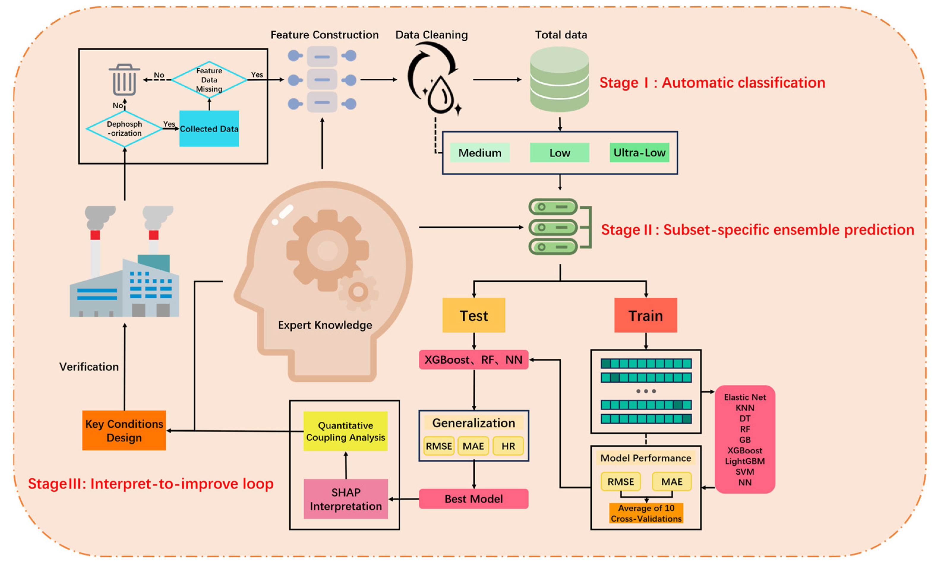
Figure 1 summarizes both the modeling workflow and its practical use in BOF operation: process and material data are first assigned to the corresponding operating domain, after which the matched subset-specific model provides endpoint phosphorus prediction and SHAP-based decision support. Nine commonly used ML algorithms were selected to predict the BOF endpoint phosphorus content [70,71]: (i) Elastic Net, (ii) K-nearest neighbor (KNN), (iii) decision tree (DT), (iv) RF, (v) gradient boosting (GB), (vi) XGBoost, (vii) LightGBM, (viii) support vector machine (SVM), and (ix) NN. These candidate models were first screened on the training set of each data category, and 10-fold cross-validation was used to evaluate their performance, with the mean RMSE and MAE adopted as the primary evaluation criteria. Based on this first-stage comparison, RF, XGBoost, and NN were retained as representative high-performing models for further optimization and comparative analysis.

All models in this study were implemented in Python 3.7 using the scikit-learn library. Hyperparameter tuning was carried out by grid search, and the computations were performed on a Windows 10 system equipped with an Intel Core i5-11400 CPU (2.50 GHz).

For the selected models, hyperparameter tuning was conducted by grid search on the training set. The resulting optimal models were then applied to the independent test set for final evaluation, and the corresponding RMSE, MAE, and HR values were computed. In addition, repeated random-split experiments were further conducted for the ULP subset as a robustness check under limited data conditions.

2.2.3. Interpret-to-Improve Loop

After determining the optimal model for each category, SHAP analysis was performed on the data from each category. The SHAP results for different categories were compared to analyze the differences. SHAP is an explainability method based on game theory that calculates the contribution of each feature to the prediction outcome, revealing the impact and specific contribution of each feature on the model’s decision-making process. Compared with local explainable AI methods, such as local interpretable model-agnostic explanations, SHAP provides theoretically consistent feature attributions at both local and global levels, making it more suitable for comparing the dominant metallurgical factors across the MP, LP, and ULP operating domains. The formula for SHAP is as follows in Equation (15):

$$g\left(z^{\prime }\right)={\mathrm{\varnothing }}_0+{\displaystyle {\sum }_{j=1}^M}{\mathrm{\varnothing }}_j,$$

(15)

where $g$ is the explanation model, $M$ is the number of input features, ${\mathrm{\varnothing }}_j$ represents the attribution value (Shapley value) of each feature, and ${\mathrm{\varnothing }}_0$ is a constant.

Further quantitative feature interaction SHAP analysis was performed. By analyzing the quantitative coupling SHAP values between multiple features, the unique metallurgical principles in the ULP dephosphorization process were revealed. Such a process provides guidance for more precise control of ULP removal in industrial applications.

2.3. Experimental Verification

Based on the iDePP results, combined with expert knowledge and the actual production conditions used in industry, key process parameters for the smelting of ULP-HPFe were designed (detailed in Section 3.4). Industrial-scale experimental verification was carried out on a 200-ton BOF production line. Various characterization methods, including inductively coupled plasma mass spectrometry (ICP-MS), atomic absorption spectroscopy (AAS), and infrared (IR) absorption spectrometry, were used to precisely measure the elemental composition of the high-purity iron samples. The microstructure of the high-purity iron samples and the distribution of inclusion elements were studied using a Phenom XL scanning electron microscope (SEM) equipped with energy dispersive spectroscopy (EDS).

It should be noted that the present framework is intended mainly as an offline analysis and decision-support tool rather than a fully automated online routing system. In actual BOF production, the target steel grade and phosphorus control requirement are usually determined in advance according to the customer order, so experienced engineers can generally judge qualitatively whether a heat belongs to the LP or ULP route and then select the corresponding domain-specific model.

3. Results and Discussion

3.1. Data Preprocessing Results

3.1.1. Data Cleaning and Automatic Classification

A total of 5102 records of process data from the BOF dephosphorization process were collected from industry. The data included charging conditions, process parameters, and other process data, with the phosphorus content at the BOF endpoint as the target label. Using Equations (1)–(9), derived features, such as charge material weight per ton of steel, gas flow per ton of steel, CaO content, and basicity, were calculated. These features played a crucial role in the subsequent ML process. The collected raw data were cleaned by removing data with missing values and eliminating extreme outliers based on the proportion of anomalies. After this processing, the distribution of features and target data was examined to see if it approximates a normal distribution. Figure S1 shows the distribution density plots before and after data cleaning. The cleaned data showed more regular distributions, supporting stable model training in the subsequent analysis.

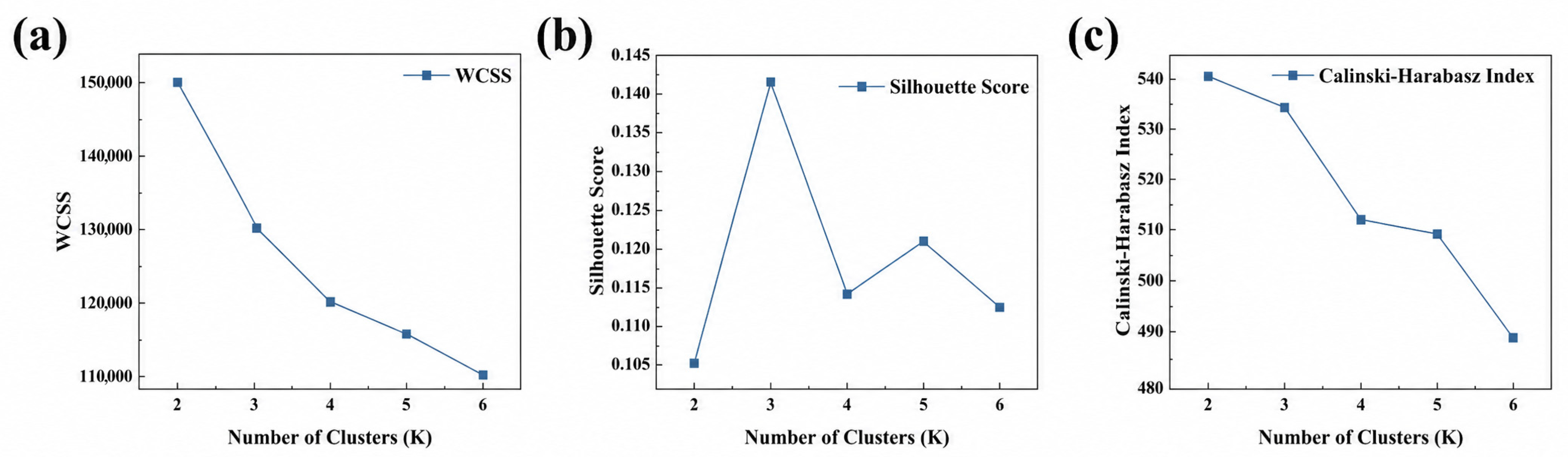
To determine the optimal number of clusters, K values from 2 to 6 were evaluated using the WCSS, the Silhouette coefficient, and the CH index, as shown in Figure 2. The results indicate that K = 3 achieved the highest Silhouette coefficient (0.14167), while its CH value (534.54) remained very close to that of K = 2 (540.80). Meanwhile, the WCSS decreased substantially from 150,166.52 at K = 2 to 129,777.69 at K = 3, indicating that introducing the third cluster significantly improved compactness.

Although the Silhouette coefficient of 0.14167 indicates partial overlap among the clusters and the CH index slightly favors K = 2, K = 3 was retained because it provides a clear reduction in WCSS and yields three operationally distinguishable domains with different phosphorus distributions, feature sets, and prediction responses.

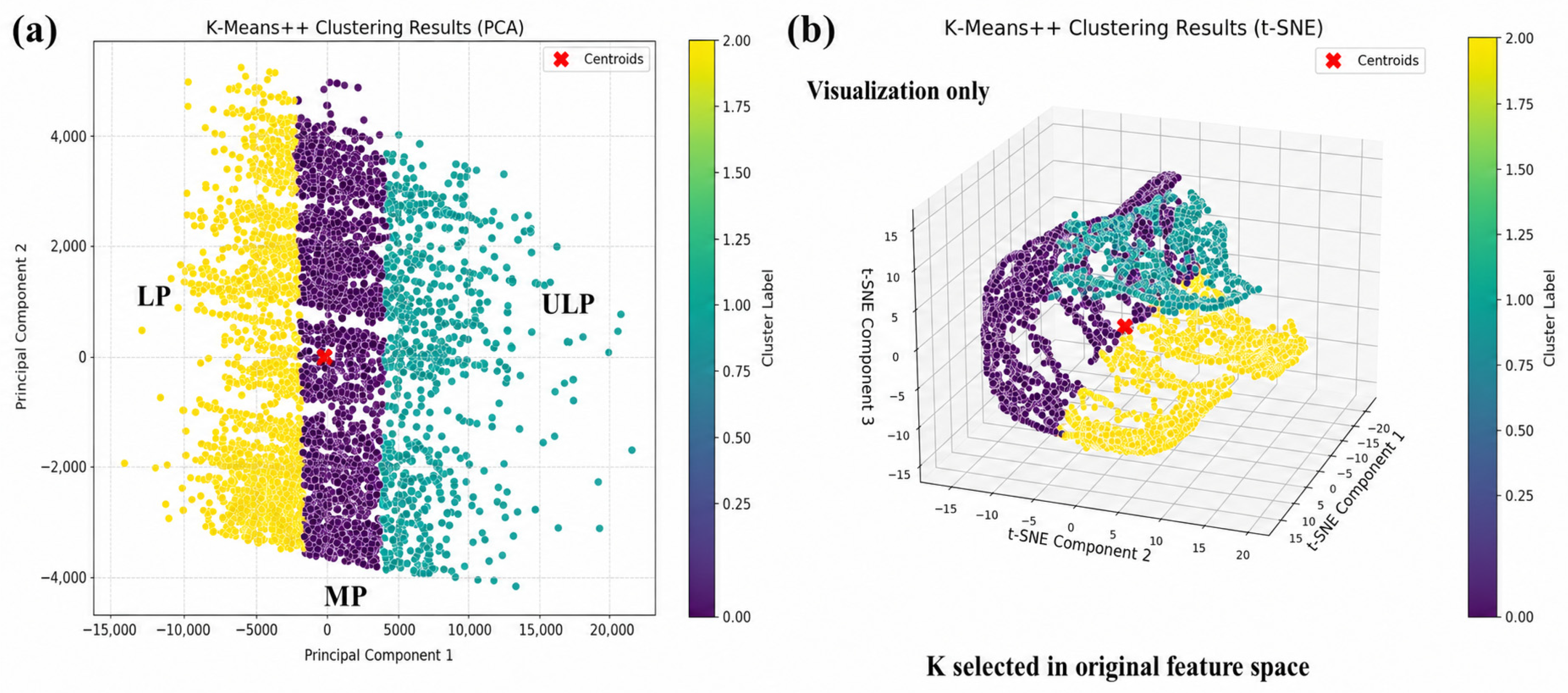
After determining K = 3 by quantitative evaluation in the original feature space, PCA and t-SNE were further used only for low-dimensional visualization of the obtained partitions, as shown in Figure 3. In the PCA projection, the three groups still exhibit partial overlap, which is expected when high-dimensional industrial data are projected onto two dimensions.

In contrast, the t-SNE projection shows a clearer visual separation. However, these visualizations are used only for qualitative illustration rather than as the basis for clustering validation. The actual partition quality was evaluated in the original feature space using internal clustering metrics. By applying iDePP to partition the raw data, three clusters were automatically obtained. Expert comparison showed that these clusters align well with conventional metallurgical categories—iDePP-MP (primarily Q235, Q345 steel, etc., with phosphorus content at the BOF endpoint in the medium range), iDePP-LP (primarily X42-X70 steel, with phosphorus content in the lower range), and iDePP-ULP (primarily FS, TLS steel, etc., with phosphorus content at the BOF endpoint in the ultra-low range). These results suggest that the three clusters should be interpreted as partially overlapping operating domains rather than completely separated natural classes, while their distinct process characteristics and downstream prediction performance support their practical metallurgical relevance.

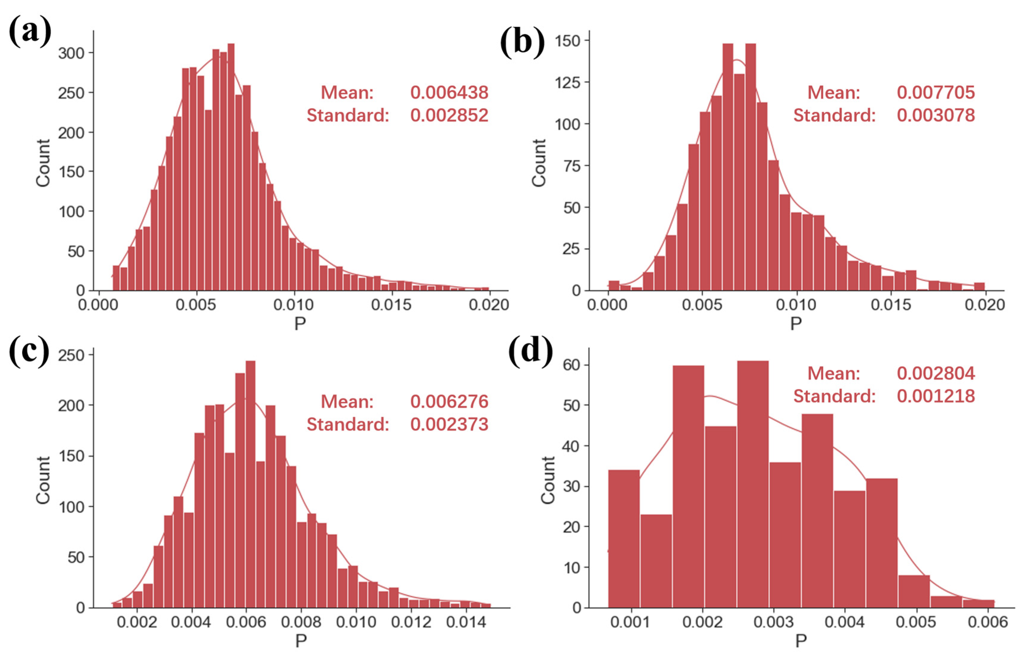
After partitioning, each subset was cleaned separately. Figure S2 shows the distribution of feature data for each steel category after cleaning. Figure 4 shows the distribution of label data for each steel category after cleaning. As shown in Figure 4b–d, the average phosphorus content of iDePP-MP at the end of the converter is approximately 77 ppm, iDePP-LP has an average phosphorus content of about 62 ppm at the end of the converter, and iDePP-ULP has an average phosphorus content of about 28 ppm at the end of the converter.

For the different phosphorus content categories in this study, based on the distribution density of the endpoint phosphorus content in each category, the hit error ranges for each type of steel are as follows [38,39,47]. iDePP-MP: a prediction is considered a hit when the difference between the predicted and actual values is within ±0.002%, iDePP-LP: a prediction is considered a hit when the difference between the predicted and actual values is within ±0.0015%, and DePP-ULP: a prediction is considered a hit when the difference between the predicted and actual values is within ±0.0006%.

After classification, all three data categories still exhibit a normal distribution, indicating that the target phosphorus values of the three steels overlap to some extent within the overall dataset. The iDePP-ULP subset represents the lowest-phosphorus operating domain identified from multidimensional process variables rather than a group defined exclusively by the threshold p < 20 ppm. Its mean value of approximately 28 ppm, therefore, reflects the inclusion of both near-target and sub-20-ppm heats, while also indicating that the most critical sub-20-ppm region remains relatively underrepresented. Therefore, if the three types of steel are grouped together or training is based solely on composition, the prediction accuracy may not reach the desired value (as detailed in Section 3.2). This finding further underscores the advantage of iDePP in handling complex industrial scenarios [69].

3.1.2. Feature Engineering

To eliminate redundant features and improve the model’s predictive capability, correlation and importance analyses were performed on the cleaned data for all three categories where the Pearson correlation coefficient method was used to calculate the correlations between features [72]. The correlations between features and their importance to the target are shown in Figure S3. It can be seen that some features have strong correlations (with absolute values greater than 0.8), indicating that these features may carry similar information. For example, in the iDePP-MP, the correlation between Al_Charge and Al₂O₃ content is 1.0, indicating that the contributions of these two features are redundant. Therefore, the less important Al_Charge feature was removed. Additionally, while the correlation between N₂_Total and N₂_Main is low, according to expert knowledge, continuous oxygen blowing is required throughout the BOF refining process, and N₂_Total is considered a more influential feature on the endpoint phosphorus content, while N₂_Main was discarded. After feature selection based on correlation analysis, feature importance, and expert knowledge [68], the numbers of remaining features were as follows: Global, 27, iDePP-MP, 27, iDePP-LP, 24, and iDePP-ULP, 18.

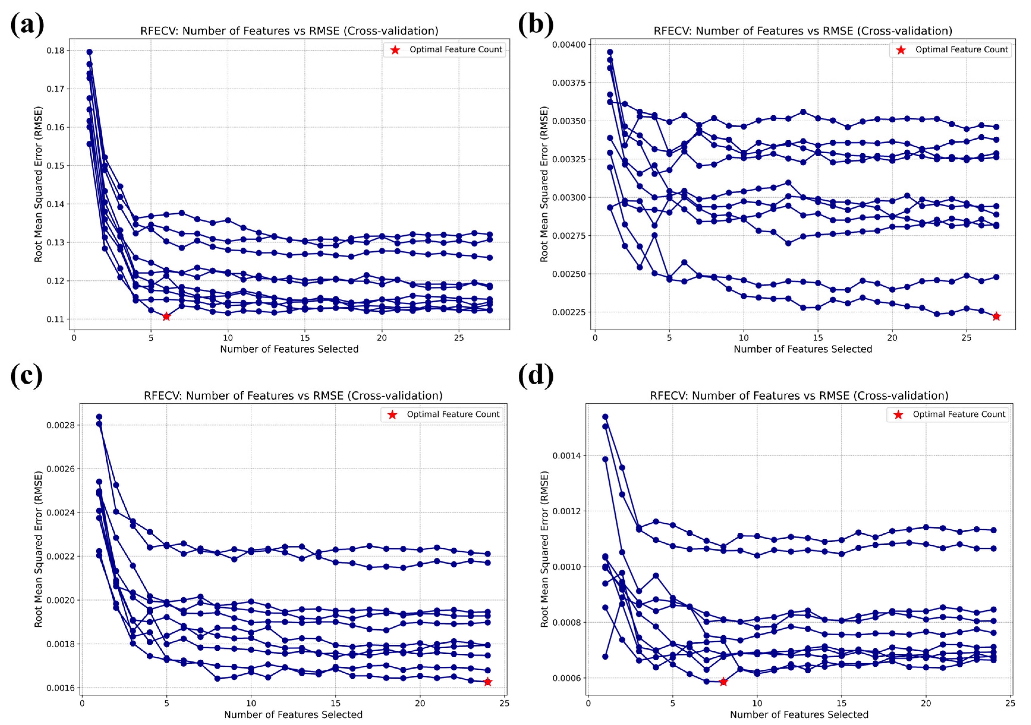
Finally, the three types of data underwent RFEcv to further optimize the feature set. Through 10-fold cross-validation, the optimal feature sets (with the lowest RMSE) for each data type were selected. The RFEcv process curves for each data type are shown in Figure 5, where the red pentagram markers indicate the optimal feature sets. The optimal numbers of features for the global baseline, iDePP-MP, iDePP-LP, and iDePP-ULP were 6, 27, 24, and 8, respectively. The compact ULP feature set suggests that, under extremely low-phosphorus requirements, many conventional factors have reduced marginal influence, while a limited number of critical variables become dominant in controlling further dephosphorization.

After cleaning and partitioning, the remaining data volumes for iDePP-MP, iDePP-LP, and iDePP-ULP are 1460, 2803, and 392 heats, respectively. Although the iDePP-ULP subset contains only 392 heats, model complexity was controlled through RFECV, cross-validation, and independent test-set evaluation. Additional repeated-split analyses were also conducted to assess the robustness of the model, as discussed later in Section 3.2. The final feature names and data details for each category after feature processing are provided in

Table 2. Optimal feature sets and total data volume for each category.

Category	Feature	Data Volume
Global	C_0, Steel_0, Age, Time_Blow, N2_Total, N2_Main	4658
iDePP-MP	C_0, P_0, S_0, Dust, Ore, C_Charge, Dolomite_Raw, Lime, Limestone, Fe-Si_Charge, Steel_Scrap, MgO, Al2O3, SiO2, CaO%, MgO%, Basicity, Temperature_0, Temperature_1, Steel_0, Steel_1, Age, Time_Blow, O2_Main, N2_Total, Ar_Total, Slag	1460
iDePP-LP	C_0, P_0, S_0, Dust, Ore, C_Charge, Dolomite_Raw, Lime, Limestone, Fe-Si_Charge, Steel_Scrap, Al2O3, SiO2, Basicity, Temperature_0, Temperature_1, Steel_0, Steel_1, Age, Time_Blow, O2_Total, N2_Total, Ar_Total, Slag	2803
iDePP-ULP	Lime, Limestone, Temperature_1, Steel_0, Age, Time_Blow, O2_Total, Slag	392

.

3.2. Results of Model Training and Evaluation

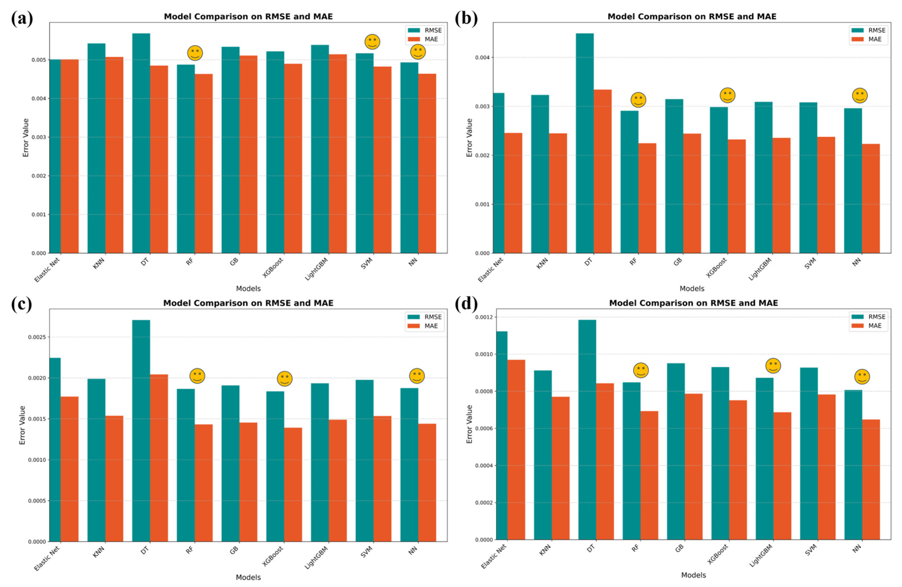
Nine common models were selected for 10-fold cross-validation training on the training set, with RMSE and MAE from the validation set used as evaluation metrics. The training results are shown in Figure 6, where smile icons denote the better-performing models among the nine candidates. Figure 6a shows the global baseline results, in which RF, SVM, and NN achieved the best performance. Figure 6b presents the training results for iDePP-MP, with the most effective models being RF, XGBoost, and NN. Figure 6c displays the training results for iDePP-LP, with RF, XGBoost, and NN being the optimal models. Figure 6d illustrates the training outcomes for iDePP-ULP, with RF, LightGBM, and NN being the most effective models.

Considering the results across all subsets together, RF, XGBoost, and NN were retained as the representative models for further optimization and comparison. These three models were selected not because each of them was always the single best-performing candidate in every subset, but because they consistently showed competitive performance and, at the same time, represented complementary nonlinear learning strategies. The final model for each subset was then determined by its comprehensive performance on RMSE, MAE, and HR after optimization, which resulted in XGBoost being selected for iDePP-ULP.

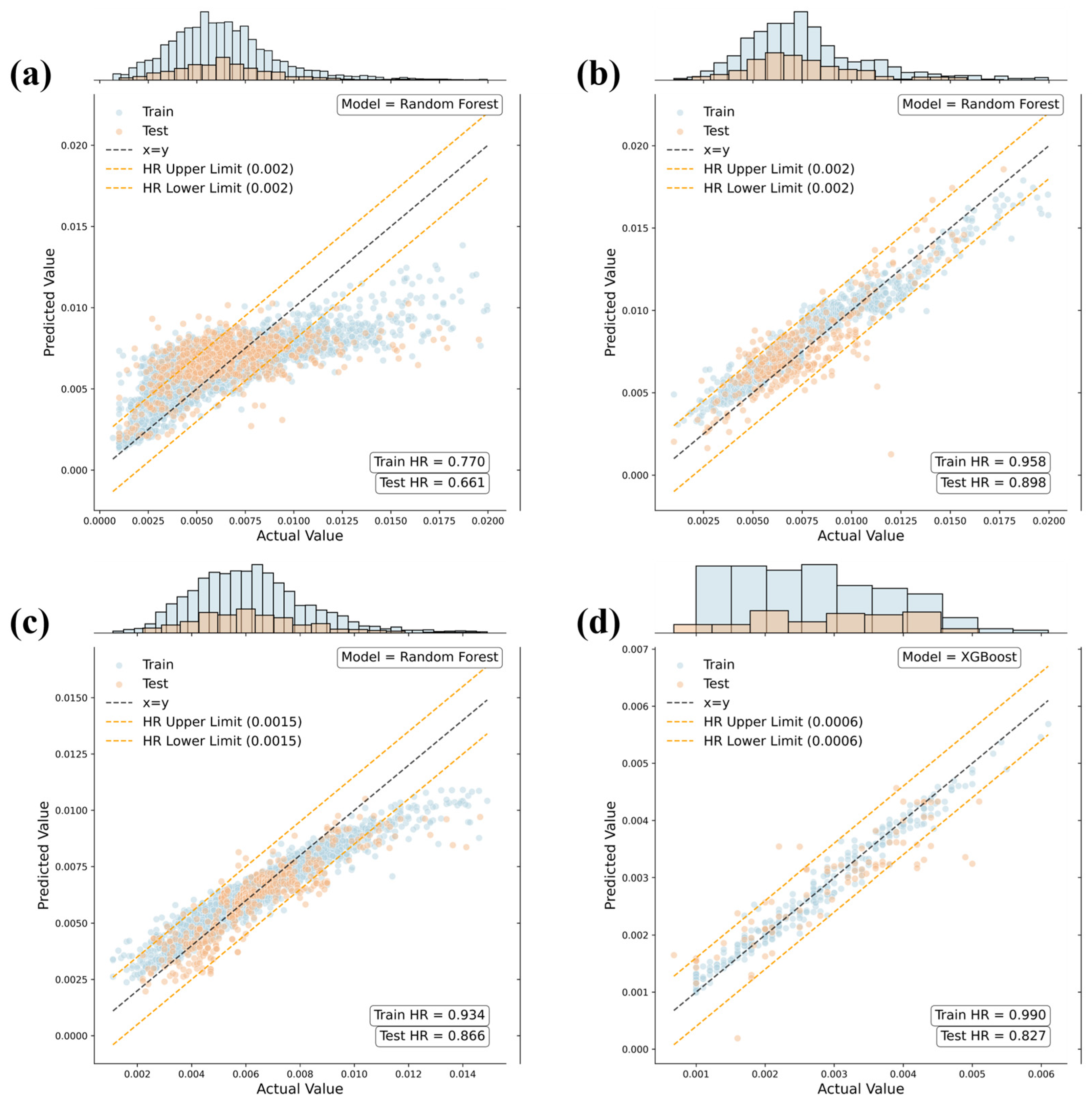
Figure 7 further illustrates the performance of each optimal model after hyperparameter optimization. In Figure 7 the horizontal and vertical axes represent the actual values of the data and the model’s predicted values, respectively. The blue scatter points represent the results from the training set, while the orange scatter points represent the results from the test set.

The orange dashed line indicates the HR hit range, and the histograms above the scatter plot represent the data distributions of the training and test sets, respectively. From the graphs it is evident that the training and test sets have similar distributions, which validates the model’s generalizability and reliability. Figure S5 presents the performance of two additional models on each data category.

The comparison shows that model performance varies across the different data categories. Specifically, the RF model performs exceptionally well on the iDePP-MP and iDePP-LP, with test set metrics of 0.0015%, 0.0011%, and 89.9%, and 0.0011%, 0.0007%, and 86.6%, respectively. The advantage of RF lies in its ability to handle high-dimensional features and reduce the risk of overfitting through ensemble learning. On the other hand, the XGBoost model shows stronger advantages with respect to the iDePP-ULP, with test set metrics of 0.0005%, 0.0004%, and 82.7%. XGBoost performed best for the iDePP-ULP subset, likely because its boosting structure effectively captures nonlinear relationships in the compact feature set. The optimal parameters and evaluation results for the three models are detailed in Table S1.

Most importantly, comparing Figure 7a with Figure 7b–d clearly shows that iDePP shows improved predictive performance over the current global baseline. Compared with a single global predictor, iDePP reduces the mean absolute error from 0.0018% to 0.0011%, 0.0007%, and 0.0004% for the three classes and raises the iDePP-ULP HR to 82.7% within ±6 ppm. These findings suggest the benefit of partition-based modeling for this industrial task.

To assess whether the reported performance depended on a particular random split, 30 repeated train/test evaluations were conducted for the iDePP-ULP subset (

Table 3. Stability analysis of iDePP-ULP based on 30 repeated random splits (test-set results).

Metric	Mean	Standard Deviation	Minimum	Maximum	95%CI
RMSE	0.000481	0.000017	0.00045	0.000510	0.000474–0.000487
MAE	0.000409	0.000012	0.00039	0.00043	0.000404–0.000413
HR	0.836	0.005821	0.826	0.846	0.833827–0.838173

). The narrow standard deviations and 95% confidence intervals of RMSE, MAE, and HR indicate stable predictive performance across different data partitions. In addition, the RF-based control experiment using identical raw features showed that the partition-based model consistently outperformed the global baseline, providing complementary evidence that the improvement originates from domain partitioning rather than feature engineering alone.

To isolate the effect of domain partitioning from that of feature count differences, an additional RF-based control experiment was conducted using the same cleaned raw input features for both the global and partition-based models, without extra feature engineering. As shown in Figure S6, the models developed without feature engineering consistently exhibited inferior performance across all subsets compared with the corresponding RFECV-based models. These results indicate that domain partitioning improves prediction performance, while feature selection and model optimization further enhance the predictive capability of the proposed framework.

In this broader sense, the present framework is also aligned with recent industrial machine learning studies that emphasize domain-aware modeling and robust knowledge extraction under heterogeneous and data-limited conditions, even though the specific application scenarios differ [73,74,75]. It should be noted that the present models are applicable primarily within the operating domain represented by the available single-line dataset. Their direct transfer to other BOF shops, steel grades, furnace capacities, or raw material systems requires external validation and, where necessary, model recalibration.

3.3. SHAP Value Analysis Results

Recent SHAP-based studies in industrial prediction have likewise shown that interpretability is valuable not only for ranking influential variables, but also for linking model behavior to physically meaningful process patterns [76,77,78]. To validate the model’s rationality and interpretability, and to further explore the impact of each feature on phosphorus content prediction, this study conducted a SHAP analysis on the optimal models for each data type. SHAP analysis suggests the contribution of each feature to the final prediction, thereby elucidating the model’s decision-making process. Based on the results of the SHAP analysis, a feature coupling quantitative analysis was conducted by comparing the SHAP analyses and multi-feature interaction results of three different types of dephosphorization processes. The results of this analysis enabled the exploration of distinctive metallurgical characteristics associated with the ULP smelting process, ultimately providing a quantitative analysis for the design of key parameters in the ULP BOF dephosphorization process. It should be noted that the SHAP analysis in this study was used primarily as an interpretive tool to analyze model-consistent metallurgical patterns, rather than as a formal statistical inference framework.

3.3.1. Feature Interpretation

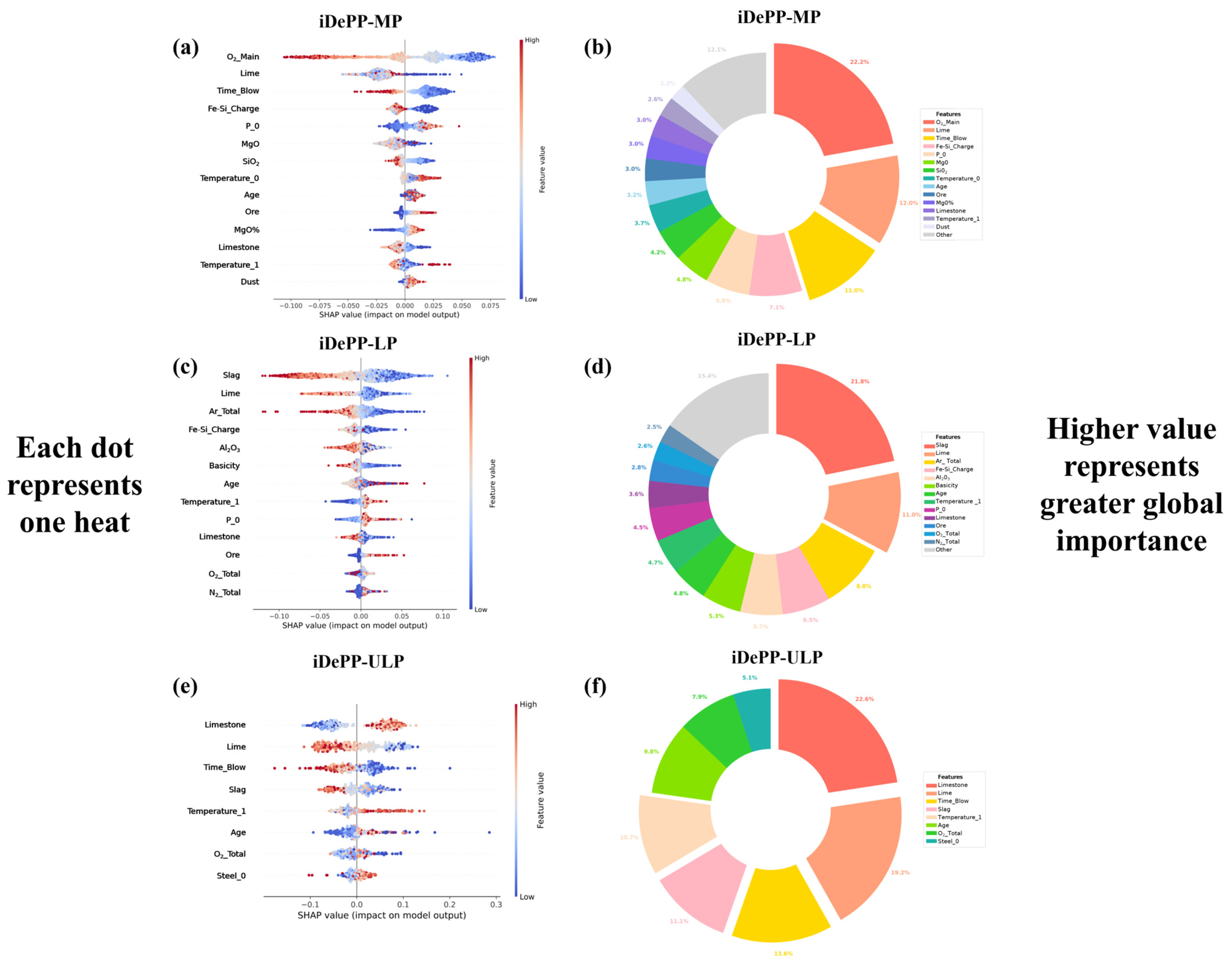
The summary of the SHAP analysis and feature absolute importance for each data type is shown in Figure 8. For the three types of SHAP results, only features with significant contributions are plotted, while scatter features with irregular distributions on the extreme sides are omitted. In Figure 8a,c,e, each point represents a data sample, with the color indicating the magnitude of the corresponding feature. The horizontal axis represents the SHAP value for each data point, where negative values indicate a negative contribution to the target, and positive values indicate a positive contribution. A value of zero indicates no contribution. For example, in Figure 8a, as the value of O₂_Main increases, it has a more negative contribution to the final phosphorus content. For the medium-phosphorus regime, increasing the oxygen supply was associated with a lower endpoint phosphorus content:

$$\begin{array}{c}2\left[P\right]+5\left(FeO\right)+3\left(CaO\right)= \left(3CaO·P_2{O}_5\right)+5\left\{Fe\right\} \\ \Delta G^0=\left(-832.302+318.67T\right) \mathrm{J}/\mathrm{mol}\end{array}$$

(16)

$$In \left(\%P_{eq}\right)={\displaystyle \frac{1}{2}}In\left(a_{3CaO·P_2{O}_5}\right)+{\displaystyle \frac{\Delta G^0}{2RT}}-{\displaystyle \frac{{5\mu }_{O_2}}{4RT}}-{\displaystyle \frac{3In\left(a_{CaO}\right)}{2}}-In\left(f_p\right).$$

(17)

Equation (16) [79] represents the dephosphorization reaction equation, where phosphorus is oxidized and combines with CaO, forming a slag from which it is removed. According to the Gibbs free energy change, the dephosphorization reaction is exothermic. Equation (17) [79] contains the expression derived from the reaction equation that describes the factors affecting dephosphorization efficiency. From the three types of SHAP summary plots, it is clear that the features, such as P_0, Lime, O₂_Main, Basicity, and Temperature_1, are broadly consistent with the well-established dephosphorization reaction mechanisms. For example, the dephosphorization reaction is promoted by increased oxygen supply and lower temperature, consistent with established metallurgical principles. This finding supports the interpretability and reliability of the model. These metallurgical theories have been extensively studied and have achieved a relatively unified understanding. Therefore, this work focuses on further analyzing the unique parameters derived from ML. As shown in Figure 8, for the iDePP-MP and iDePP-LP, the contribution of P_0 is significant, while for the iDePP-ULP, P_0 has almost no effect. This anomaly arises because, for iDePP-ULP, the final phosphorus content is already very low. From a reaction kinetics perspective, the reaction is approaching its saturation limit, and the driving force provided by P_0 decreases, no longer playing a decisive role in controlling the reaction rate or further forward progression. A similar consideration applies to O₂_Main. In the iDePP-MP, O₂_Main is the primary contributing feature, whereas in iDePP-LP and iDePP-ULP, O₂_Main has become a redundant factor, but Ar_Total has a greater impact on phosphorus removal. At the same time, an unexpected performance of age is observed, which is a feature rarely considered in previous studies. As seen in the SHAP summary plots for iDePP-MP and iDePP-LP in Figure 8a,c, the blue and red scatter points in the age category are unevenly distributed on both sides of the baseline, showing no obvious contribution. However, in the SHAP summary analysis for iDePP-ULP in Figure 8e, age appears to be a significant factor for further deep dephosphorization. As the age value decreases, the final phosphorus content in the BOF reduces. This anomaly may be due to the fact that a longer furnace aging time implies a higher number of usage cycles that leads to negative outcomes, including erosion and deformation of the furnace wall, deterioration of the permeability of the refractory bricks, and a decline in the bottom-blown stirring effect. Meanwhile, as the permeable bricks encasing the bottom-blowing tuyeres become partially clogged with age, gas dispersion becomes non-uniform, shifting the converter operation from combined top-and-bottom blowing to top-blowing only. Consequently, there is a reduction in the contact area between the slag and molten steel, which results in a reduced dephosphorization reaction area in terms of kinetics. Such behavior leads to incomplete and insufficient dephosphorization. Therefore, in the ULP steelmaking process where phosphorus requirements are extremely low, aging has a significant impact. Additionally, changes in the furnace shape also affect the subsequent slag tapping efficiency.

A notable finding for iDePP-ULP is that increased limestone addition is associated with higher endpoint phosphorus, contrary to the conventional expectation. As shown in Figure 8e, with an increase in the amount of limestone added the final phosphorus content actually increases, which negatively impacts dephosphorization. This opposite phenomenon may be because, as the phosphorus purity requirements increase, the temperature control of the entire BOF process becomes extremely stringent. The decomposition of CaCO₃ in limestone into CaO and CO₂ is an endothermic reaction, which puts thermal pressure on the ULP process where there is no excess temperature:

$${CaCO}_3\to CaO+{CO}_2, \Delta H°\approx 178 \mathrm{k}\mathrm{J}·{\mathrm{m}\mathrm{o}\mathrm{l}}^{-1}.$$

(18)

To provide quantitative support for the SHAP-derived interpretation of the limestone-induced thermal penalty, a simplified thermodynamic estimation was further introduced. As shown in Equation (18) [80], limestone decomposition proceeds through an endothermic reaction. Since the molar mass of CaCO₃ is about 100.09 g·mol⁻¹, the decomposition of 1 kg of limestone requires approximately 1.78 MJ of heat. For 1 t of molten steel, assuming an effective heat capacity of about 0.84 kJ·kg⁻¹·K⁻¹, this is equivalent to an approximate thermal penalty of 2.12 °C per kg of limestone [81]. Accordingly, an additional 5–10 kg/t steel of limestone would introduce an extra heat demand of about 8.9–17.8 MJ/t steel, corresponding to an equivalent temperature loss of about 10.6–21.2 °C. Under the relatively narrow thermal margin of the ULP route, such an additional thermal burden may become non-negligible and thus could adversely influence slag formation and endpoint dephosphorization efficiency [82].

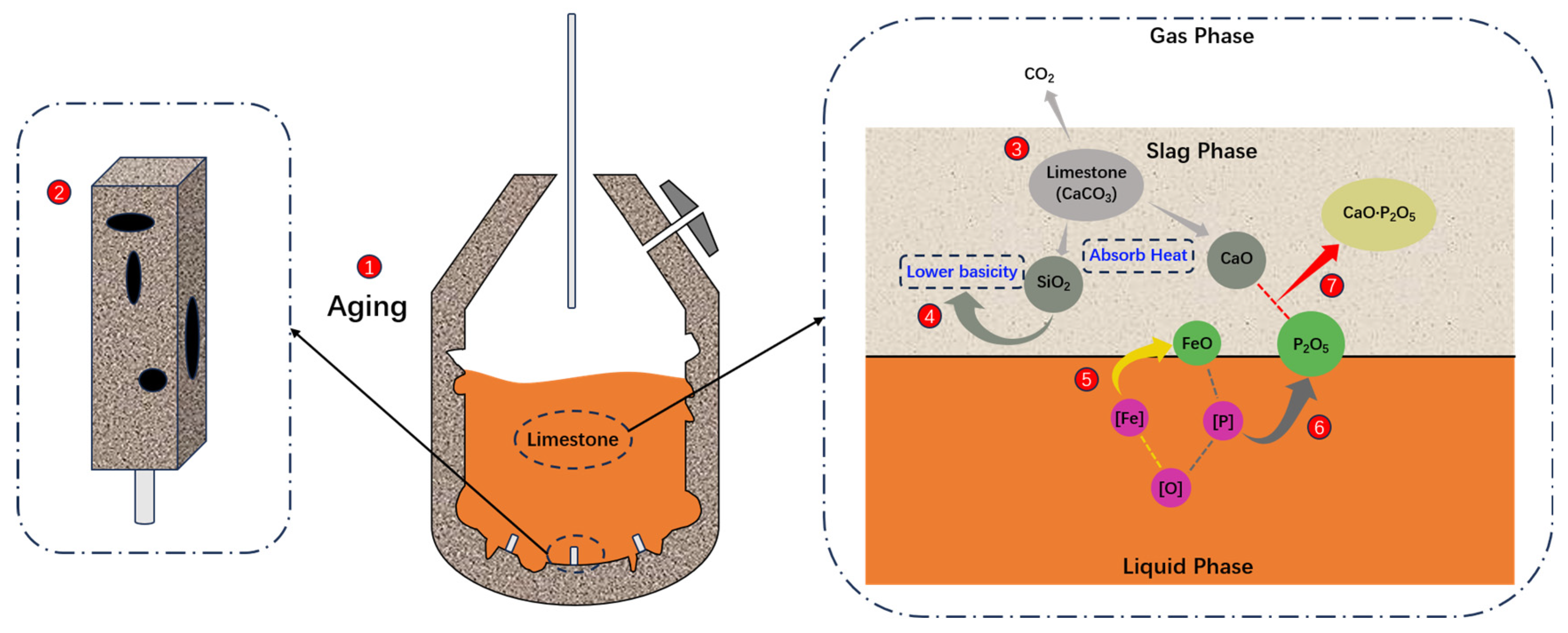
At the same time, limestone contains a relatively high amount of SiO₂, which when entering the slag, lowers the basicity of the steel slag such that it affects the dephosphorization efficiency. Therefore, for the ULP steelmaking process, it is essential not to consider only the cost of the added materials in isolation. The schematic diagram of the unique dephosphorization process mechanism and key influencing factors for the iDePP-ULP is shown in Figure 9.

3.3.2. Feature Coupling Analysis

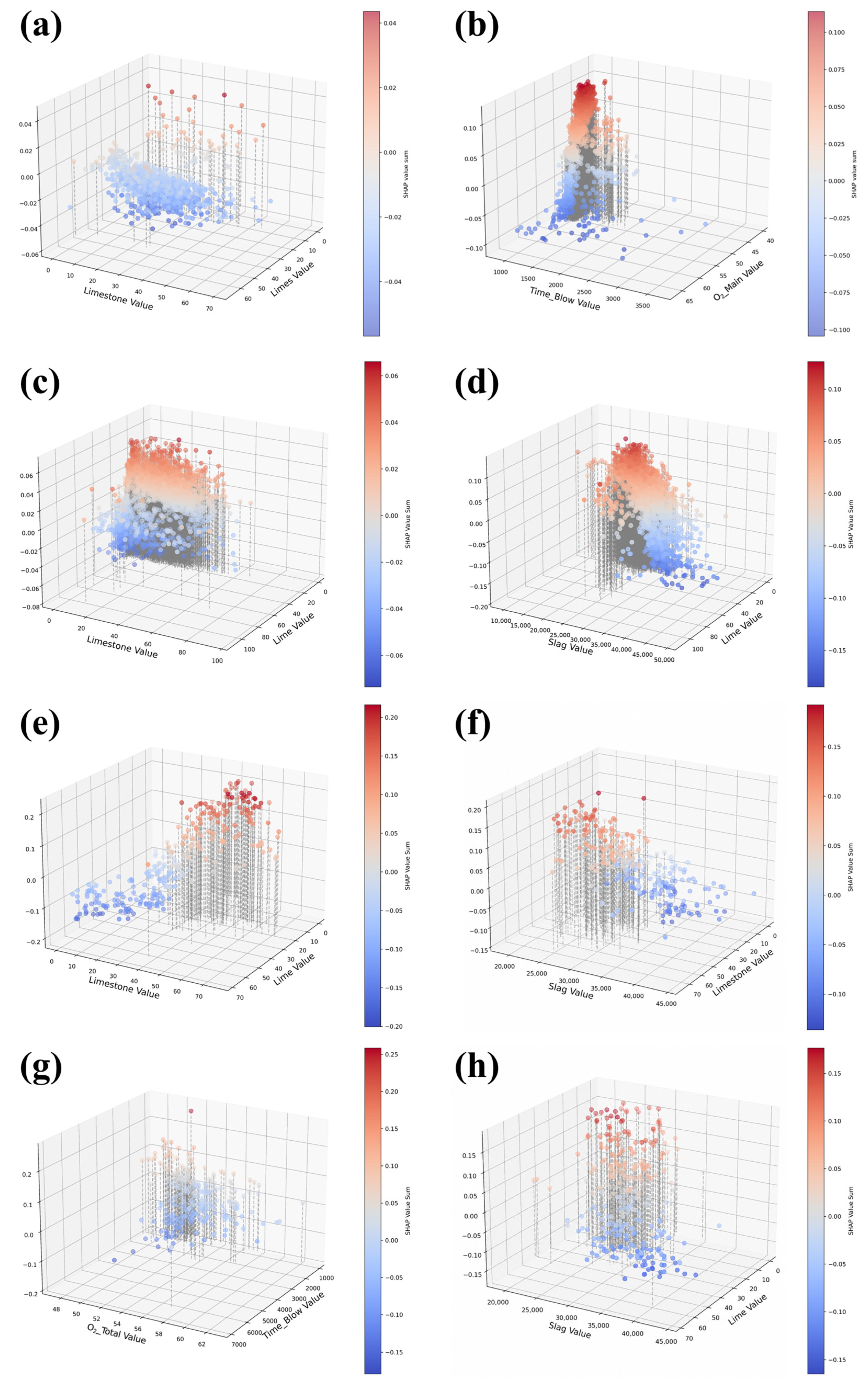
To further quantify the relationships among limestone, lime, slag, Time_Blow, and O₂_Main, feature coupling analysis was performed based on their SHAP contributions. Based on the feature importance analysis, a quantitative analysis of the interactions between features was conducted. In the present study, the quantitative feature coupling analysis was focused mainly on the ULP subset, with the aim of identifying practically meaningful proportional relationships and operating ranges among the key variables, rather than conducting formal significance testing of the interactions themselves. As shown in Figure 10, the horizontal axis represents the actual values of different features, while the vertical axis represents the sum of the SHAP values of the two features (for example, the scatter point in Figure 10a represents the sum of SHAP values of limestone and lime). The color of the scatter points represents the magnitude of the sum of the SHAP values, where red points represent a total SHAP value greater than 0 and blue points represent a total SHAP value less than 0.

As seen in Figure 10a,c,e, for the iDePP-MP, the proportion of limestone has no obvious positive or negative contribution to the dephosphorization results. As the total amount of lime and limestone increases, dephosphorization proceeds positively, with lime not being in excess and playing a primary role in the reaction. For iDePP-ULP, the lowest combined SHAP values occurred when lime was approximately 40–60 kg/t and limestone was approximately 0–10 kg/t. In this scenario the total SHAP value reaches its minimum. Furthermore, the scatter points show a distinct bimodal peak, further confirming the earlier discussion that for ULP dephosphorization, the proportion of limestone in the lime should remain small. This trend is consistent with the newly identified dephosphorization mechanism for the iDePP-ULP regime: as the phosphorus purity requirement becomes more stringent, the BOF process is operated with an extremely narrow temperature margin.

Next, the optimal distribution of limestone and lime in the slag was analyzed (see Figure 10d,f,h), and it was determined that the dephosphorization effect is best when slag exceeds 40,000. For limestone and lime, in both the iDePP-LP and iDePP-ULP, the results indicated that the proportion of limestone should be as small as possible, with an optimal contribution range (the proportion of limestone in the total lime volume is ≤20%). In this case, the slag volume and temperature are sufficient to dissolve most of the added lime, forming a more homogeneous, CaO-rich liquid slag matrix that is microstructurally favorable for P₂O₅ dissolution and diffusion.

As seen in Figure 10b,g, for the iDePP-MP when O₂ is not in excess, Time_Blow shows no significant contribution range. However, in the iDePP-ULP when O₂ is in excess, the positive contribution to dephosphorization increases as Time_Blow increases. At the same time, Time_Blow also has an optimal range (3000–6000) to make the overall dephosphorization effect best. Within this window, the combination of sufficient blowing time and basic liquid slag promotes complete lime dissolution and stable phosphate formation, while avoiding excessive cooling or over-oxidation that would again leave undissolved lime and a non-uniform slag microstructure. This finding is also consistent with the reported effectiveness of double-slag dephosphorization, providing indirect support for the model interpretation [83], indirectly validating the reliability of the model.

Compared with traditional metallurgical prediction approaches [84], which are usually derived from simplified equilibrium or kinetic assumptions, the proposed iDePP framework is designed to better handle the heterogeneity, nonlinearity, and skewed distribution of real industrial BOF data. In this sense, the present method is not intended to replace metallurgical understanding, but to complement it by providing a more accurate and interpretable data-driven tool for process analysis and optimization, particularly in the ULP regime [85].

3.4. Verification Result

To validate the model’s generalizability and reliability, key parameters were designed based on the SHAP analysis and expert knowledge. Additionally, preliminary industrial validation trials were conducted using a 200-ton BOF at a metallurgical company. Chemical analysis of the final continuous-casting products was subsequently performed, with the key parameters and chemical composition shown in

Table 4. Key parameter settings, chemical composition, and model prediction errors.

Key Parameter
Age	P_0	Lime% in Limestone and Lime			Slag	O2	Time_Blow
≤600	≤0.04	≥80%			≥40,000	≥55	≥3000
Component (wt.%)
C	Si	Mn	P	S	Al	N	O
0.004	0.016	0.017	0.0019	0.0005	0.021	0.0025	0.0017
0.58	0.097	0.073	0.0012	0.004	0.0046	0.0036	0.0024
0.0026	0.006	0.016	0.0013	0.0007	0.0064	0.0038	0.0029
P_Actual_BOF			P_Predicted_BOF			error
0.0016%			0.002073%			4 ppm
0.0017%			0.001812%			1 ppm
0.0018%			0.001659%			1.5 ppm

.

Based on the coupled-feature SHAP interpretation and expert knowledge, the key operating constraints for iDePP-ULP were set as: age ≤ 600, P_0 ≤ 0.04, Lime% in (limestone + lime) ≥ 80%, slag ≥ 40,000, O₂ ≥ 55, and Time_Blow ≥ 3000, aiming at preliminary industrial verification of feasible ULP-HPFe production conditions. Under these conditions, three consecutive heats were produced, with final continuous-casting phosphorus contents of 0.0019%, 0.0012%, and 0.0013%, respectively. The corresponding BOF endpoint phosphorus contents were 0.0016%, 0.0017%, and 0.0018%, while the model achieved small absolute prediction errors of approximately 4 ppm, 1 ppm, and 1.5 ppm, respectively. Because the present industrial verification involved only three consecutive heats, the trial results are reported mainly on a per-heat basis rather than through campaign-level statistical descriptors, which would not yet be sufficiently informative at this stage.

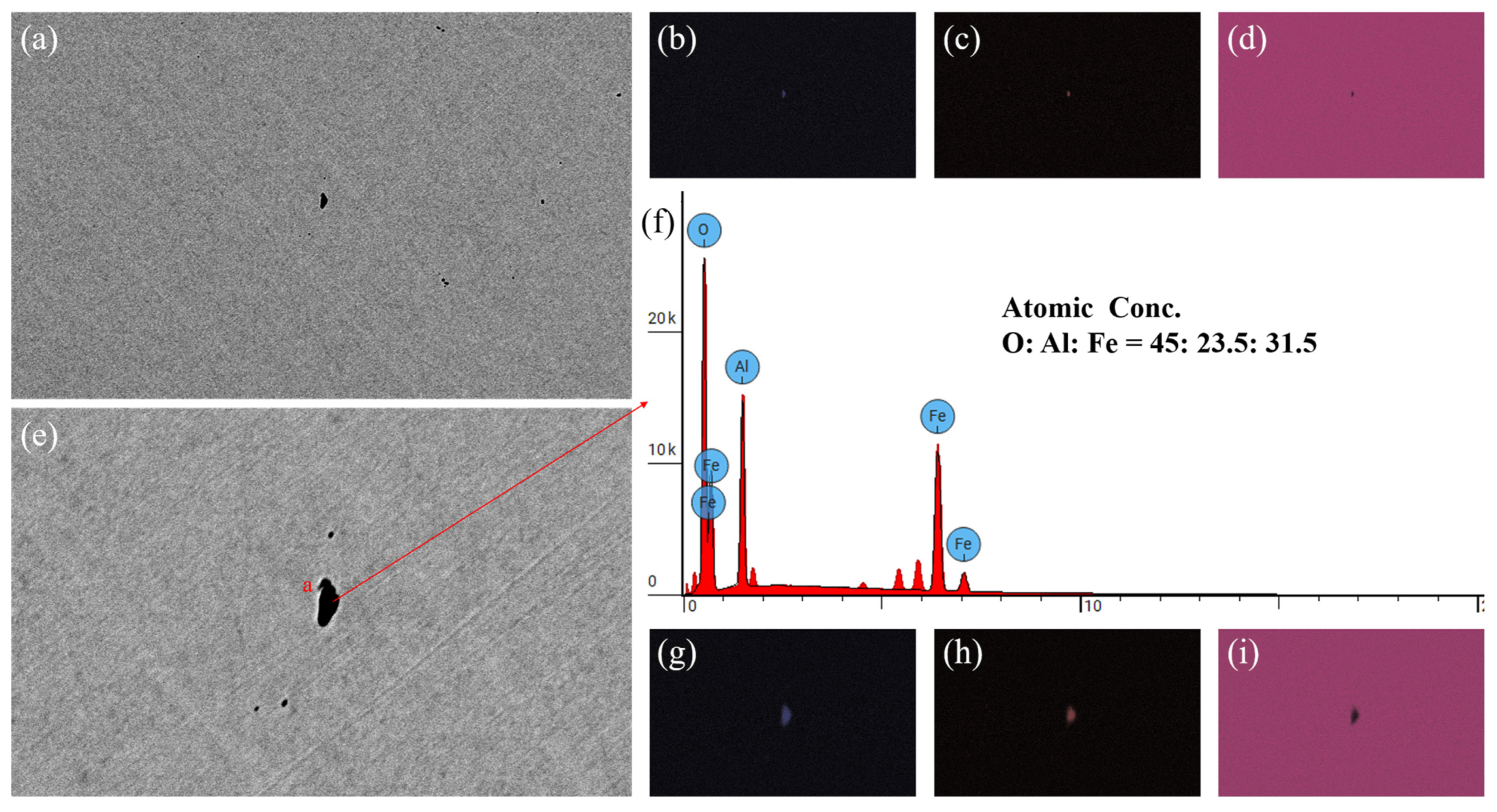
Figure 11 shows the SEM images and EDS results of the samples at a magnification of 4000×, where no inclusions are visible, while at 12,000×, rare mixed inclusions of Al₂O₃ and Fe₃O₄ are observed [86], with particle sizes ranging from 1 to 3 μm.

The verification results provide preliminary support for the industrial applicability of the framework and show that combining ML with metallurgical knowledge can identify physically meaningful process factors and practical operating guidance. These results also highlight the importance of integrating expert knowledge with data-driven modeling in complex industrial processes. These results provide a preliminary proof of industrial feasibility under the tested operating conditions. However, because the validation was limited to three consecutive heats, broader verification across different furnace ages, production campaigns, and operating conditions is still required to establish long-term robustness.

3.5. Potential Extension of the iDePP Framework

Beyond the present BOF endpoint phosphorus application, the proposed iDePP framework may also be extended to other metallurgical and data-sparse industrial processes that exhibit heterogeneous operating regimes, skewed data distributions, and strong nonlinear process–response relationships. The potential transferability of iDePP lies in its three-step structure: automatic partitioning to identify process-relevant regimes, subset-specific predictive modeling to improve local accuracy under heterogeneous conditions, and interpretability-guided analysis to extract actionable process knowledge from the trained models.

In metallurgical applications, such an approach may be particularly useful for other impurity control or endpoint prediction tasks, such as sulfur, aluminum, or oxygen control, where different product windows or refining conditions may correspond to distinct process domains. It may also be applicable to other complex process stages in steelmaking and related high-temperature manufacturing systems, especially when a single global model is insufficient to represent multiple operating regimes.

At the same time, such extension should be carried out with appropriate caution. The partitioning variables, feature-construction strategy, and process interpretation need to be redesigned according to the physical characteristics of the target system, and the resulting models may require database expansion and periodic recalibration before long-term industrial deployment. Therefore, the broader value of iDePP lies not in the direct transfer of one trained model to all tasks, but in the transferability of the partition-and-prediction methodology itself for heterogeneous and data-limited industrial problems.

4. Conclusions and Prospect

This study presented iDePP, an intelligent partition-and-prediction framework that combines unsupervised clustering, subset-specific ensemble learning, and SHAP-based interpretability to tackle ULP dephosphorization in the BOF. The findings are as follows:

• In this study, iDePP introduces automatic domain partitioning: using K-means++, it automatically mines three metallurgically recognized phosphorus intervals (iDePP-MP, iDePP-LP, and iDePP-ULP) from 5102 complex industrial records without relying on recipe thresholds, thereby demonstrating machine-learning-driven rediscovery of expert knowledge.
• Compared with a single global predictor, iDePP reduces the mean absolute error from 0.0018% to 0.0011%, 0.0007%, and 0.0004% for the three classes, respectively. Crucially, it increases the hit rate for the most difficult ULP grade to 82.7% within a strict tolerance of ±6 ppm.
• The optimal model for each category is interrogated with SHAP analysis to confirm that its explanations accord with metallurgical principles, thereby validating model reliability and interpretability. Furthermore, comparative SHAP analysis across the three categories suggests two potentially important metallurgical mechanisms for ULP dephosphorization: heat interference from limestone addition and tuyere-brick clogging accompanied lining deformation due to furnace aging.
• Based on the above analysis and the on-site operating conditions of a metallurgical company, specific key parameters were designed: age ≤ 600, P_0 ≤ 0.04, Lime% in limestone and lime ≥ 80%, slag ≥ 40,000, O₂ ≥ 55, and Time_Blow ≥ 3000. Industrial validation on a 200-ton BOF using three consecutive heats provided a preliminary verification of feasible ULP-HPFe production with prediction errors of approximately 4 ppm, 1 ppm, and 1.5 ppm, respectively.

This study suggests that automatic domain partitioning combined with subset-specific modeling offers a promising route to high-accuracy, interpretable control in data-sparse industrial processes. Future work will incorporate real-time blowing-curve features and expand the database across different BOF shops, steel grades, raw material conditions, and furnace campaigns to evaluate transferability and support model recalibration.

References

1. Abiko, K. Why Do We Study Ultra-High Purity Base Metals? Mater. Trans. 2000, 41, 233–237. [Google Scholar] [CrossRef] [Scilit]
2. Naito, M.; Takeda, K.; Matsui, Y. Ironmaking Technology for the Last 100 Years: Deployment to Advanced Technologies from Introduction of Technological Know-how, and Evolution to Next-generation Process. ISIJ Int. 2015, 55, 7–35. [Google Scholar] [CrossRef] [Scilit]
3. Lu, Z.; Liu, H.; Chen, F.; Li, H.; Xue, X. Just-in-time updated DBN BOF steel-making soft sensor model based on dense connectivity of key features. High Temp. Mater. Process. 2024, 43, 20240060. [Google Scholar] [CrossRef] [Scilit]
4. Isshiki, M.; Mimura, K.; Uchikoshi, M. Preparation of high purity metals for advanced devices. Thin Solid Films 2011, 519, 8451–8455. [Google Scholar] [CrossRef] [Scilit]
5. Nenchev, B.; Panwisawas, C.; Yang, X.; Fu, J.; Dong, Z.; Tao, Q.; Gebelin, J.-C.; Dunsmore, A.; Dong, H.; Li, M.; et al. Metallurgical Data Science for Steel Industry: A Case Study on Basic Oxygen Furnace. Steel Res. Int. 2022, 93, 2100813. [Google Scholar] [CrossRef] [Scilit]
6. Pal, S.; Halder, C. Optimization of Phosphorous in Steel Produced by Basic Oxygen Steel Making Process Using Multi-Objective Evolutionary and Genetic Algorithms. Steel Res. Int. 2017, 88, 201600193. [Google Scholar] [CrossRef] [Scilit]
7. Song, S.-y.; Li, J.; Yan, W. Intelligent Case-based Hybrid Model for Process and Endpoint Prediction of Converter via Data Mining Technique. ISIJ Int. 2022, 62, 1639–1648. [Google Scholar] [CrossRef] [Scilit]
8. Emi, T. Steelmaking Technology for the Last 100 Years: Toward Highly Efficient Mass Production Systems for High Quality Steels. ISIJ Int. 2015, 55, 36–66. [Google Scholar] [CrossRef] [Scilit]
9. Tomiyama, S.; Uchida, Y.; Mizuno, H.; Akiu, K.; Maeda, T. A novel control algorithm for dephosphorization in an LD converter. J. Process Control 2015, 25, 35–40. [Google Scholar] [CrossRef] [Scilit]
10. Iida, Y.; Emoto, K.; Ogawa, M.; Masuda, Y.; Onishi, M.; Yamada, H. Fully Automatic Blowing Technique for Basic Oxygen Steelmaking Furnace. Trans. Iron Steel Inst. Jpn. 1984, 24, 540–546. [Google Scholar] [CrossRef] [Scilit]
11. Brämming, M.; Björkman, B.; Samuelsson, C. BOF Process Control and Slopping Prediction Based on Multivariate Data Analysis. Steel Res. Int. 2016, 87, 301–310. [Google Scholar] [CrossRef] [Scilit]
12. Devlin, A.; Kossen, J.; Goldie-Jones, H.; Yang, A. Global green hydrogen-based steel opportunities surrounding high quality renewable energy and iron ore deposits. Nat. Commun. 2023, 14, 2578. [Google Scholar] [CrossRef] [Scilit] [PubMed]
13. Judge, W.D.; Paeng, J.; Azimi, G. Electrorefining for direct decarburization of molten iron. Nat. Mater. 2021, 21, 1130–1136. [Google Scholar] [CrossRef] [Scilit] [PubMed]
14. Mazumdar, D. Progress on half a century of process modelling research in steelmaking: A review. CSI Trans. ICT 2024, 12, 25–37. [Google Scholar] [CrossRef] [Scilit]
15. Dai, Y.; Li, J.; Shi, C.; Yan, W. Dephosphorization of high silicon hot metal based on double slag converter steelmaking technology. Ironmak. Steelmak. 2020, 48, 447–456. [Google Scholar] [CrossRef] [Scilit]
16. Furtado, F.A.; de-Olivé, F.L.; Alcântara, J.Z. Predictions at the blow end of the LD-KGC converter by a semi-dynamic control model. Int. J. Recent Adv. Mech. Eng. 2014, 3, 17–31. [Google Scholar]
17. Han, M.; Li, Y.; Cao, Z. Hybrid intelligent control of BOF oxygen volume and coolant addition. Neurocomputing 2014, 123, 415–423. [Google Scholar] [CrossRef] [Scilit]
18. Liang, Y.; Wang, H.; Xu, A.; Tian, N. A Two-step Case-based Reasoning Method Based on Attributes Reduction for Predicting the Endpoint Phosphorus Content. ISIJ Int. 2015, 55, 1035–1043. [Google Scholar] [CrossRef] [Scilit]
19. Sala, D.A.; Jalalvand, A.; Van Yperen-De Deyne, A.; Mannens, E. Multivariate Time Series for Data-Driven Endpoint Prediction in the Basic Oxygen Furnace. In Proceedings of the 2018 17th IEEE International Conference on Machine Learning and Applications (ICMLA), Orlando, FL, USA, 17–20 December 2018; pp. 1419–1426. [Google Scholar] [CrossRef] [Scilit]
20. Xie, J. Prospects of materials genome engineering frontiers. Mater. Genome Eng. Adv. 2023, 1, e17. [Google Scholar] [CrossRef] [Scilit]
21. Xue, D.; Lookman, T. Editorial: Shaping the future of materials science through machine learning. Mater. Genome Eng. Adv. 2024, 2, e80. [Google Scholar] [CrossRef] [Scilit]
22. Chen, J.; Liao, C.-M. Dynamic process fault monitoring based on neural network and PCA. J. Process Control 2002, 12, 277–289. [Google Scholar] [CrossRef] [Scilit]
23. Dávila-Santiago, E.; Shi, C.; Mahadwar, G.; Medeghini, B.; Insinga, L.; Hutchinson, R.; Good, S.; Jones, G.D. Machine Learning Applications for Chemical Fingerprinting and Environmental Source Tracking Using Non-target Chemical Data. Environ. Sci. Technol. 2022, 56, 4080–4090. [Google Scholar] [CrossRef] [Scilit] [PubMed]
24. Ismail, H.Y.; Fayyad, S.; Ahmad, M.N.; Leahy, J.J.; Naushad, M.; Walker, G.M.; Albadarin, A.B.; Kwapinski, W. Modelling of yields in torrefaction of olive stones using artificial intelligence coupled with kriging interpolation. J. Clean. Prod. 2021, 326, 129020. [Google Scholar] [CrossRef] [Scilit]
25. Li, Y.; Li, H.; Wang, C.; Jose Rivera-Diaz-del-Castillo, P.E. The role of physical metallurgical relationships in enhancing alloy properties prediction and design: A case study on Q&P steel. Mater. Genome Eng. Adv. 2024, 3, e70. [Google Scholar] [CrossRef] [Scilit]
26. Wang, B.; Wang, W.; Qiao, Z.; Meng, G.; Mao, Z. Dynamic selective Gaussian process regression for forecasting temperature of molten steel in ladle furnace. Eng. Appl. Artif. Intell. 2022, 112, 104892. [Google Scholar] [CrossRef] [Scilit]
27. Zhong, S.; Zhang, K.; Bagheri, M.; Burken, J.G.; Gu, A.; Li, B.; Ma, X.; Marrone, B.L.; Ren, Z.J.; Schrier, J.; et al. Machine Learning: New Ideas and Tools in Environmental Science and Engineering. Environ. Sci. Technol. 2021, 55, 12741–12754. [Google Scholar] [CrossRef] [Scilit] [PubMed]
28. Fileti, A.M.F.; Pacianotto, T.A.; Cunha, A.P. Neural modeling helps the BOS process to achieve aimed end-point conditions in liquid steel. Eng. Appl. Artif. Intell. 2006, 19, 9–17. [Google Scholar] [CrossRef] [Scilit]
29. Geng, X.; Wang, F.; Wu, H.H.; Wang, S.; Wu, G.; Gao, J.; Zhao, H.; Zhang, C.; Mao, X. Data-driven and artificial intelligence accelerated steel material research and intelligent manufacturing technology. Mater. Genome Eng. Adv. 2023, 1, e10. [Google Scholar] [CrossRef] [Scilit]
30. Ghalati, M.K.; Zhang, J.; El-Fallah, G.M.A.M.; Nenchev, B.; Dong, H. Toward learning steelmaking—A review on machine learning for basic oxygen furnace process. Mater. Genome Eng. Adv. 2023, 1, e6. [Google Scholar] [CrossRef] [Scilit]
31. Han, M.; Liu, C. Endpoint prediction model for basic oxygen furnace steel-making based on membrane algorithm evolving extreme learning machine. Appl. Soft Comput. 2014, 19, 430–437. [Google Scholar] [CrossRef] [Scilit]
32. Han, M.; Zhao, Y. Dynamic control model of BOF steelmaking process based on ANFIS and robust relevance vector machine. Expert Syst. Appl. 2011, 38, 14786–14798. [Google Scholar] [CrossRef] [Scilit]
33. Jochen, S.; Hans-Jürgen, O.; Norbert, U.; Hendrik, B.; Katharina, M. A novel data-driven prediction model for BOF endpoint. Proc. Iron Steel Technol. Conf. 2013, 1, 923–928. Available online: https://imisdev.aist.org/AISTPapers/Abstracts_Only_PDF/PR-364-089.pdf (accessed on 28 May 2026).
34. Klanke, S.; Löpke, M.; Uebber, N.; Odenthal, H.-J.; Poucke, J.V.; Deyne, A.V.Y.-D. Advanced Data-Driven Prediction Models for BOF Endpoint Detection. AISTech 2017 Proc. 2017, 1, 1307–1313. [Google Scholar]
35. Liu, H.; Wang, B.; Xiong, X. Basic oxygen furnace steelmaking end-point prediction based on computer vision and general regression neural network. Optik 2014, 125, 5241–5248. [Google Scholar] [CrossRef] [Scilit]
36. Liu, J.; Liu, H.; Chen, F.; Su, Y.; Li, H.; Xue, X. Dynamic flame feature-driven prediction model for basic oxygen furnace steelmaking endpoint carbon content based on three-dimensional multi-layer complex networks. Eng. Appl. Artif. Intell. 2025, 139, 109564. [Google Scholar] [CrossRef] [Scilit]
37. Quan, L.; Li, A.; Cui, G.; Xie, S. Using enhanced sparrow search algorithm-deep extreme learning machine model to forecast endpoint phosphorus content of BOF. Preprints 2021. [Google Scholar] [CrossRef] [Scilit]
38. Wang, H.-b.; Cai, J.; Feng, K. Predicting the Endpoint Phosphorus Content of Molten Steel in BOF by Two-stage Hybrid Method. J. Iron Steel Res. Int. 2014, 21, 65–69. [Google Scholar] [CrossRef] [Scilit]
39. Wang, H.-b.; Xu, A.-j.; Ai, L.-x.; Tian, N.-y. Prediction of Endpoint Phosphorus Content of Molten Steel in BOF Using Weighted K-Means and GMDH Neural Network. J. Iron Steel Res. Int. 2012, 19, 11–16. [Google Scholar] [CrossRef] [Scilit]
40. Wang, X.; Han, M.; Wang, J. Applying input variables selection technique on input weighted support vector machine modeling for BOF endpoint prediction. Eng. Appl. Artif. Intell. 2010, 23, 1012–1018. [Google Scholar] [CrossRef] [Scilit]
41. Bae, J.; Li, Y.; Ståhl, N.; Mathiason, G.; Kojola, N. Using Machine Learning for Robust Target Prediction in a Basic Oxygen Furnace System. Metall. Mater. Trans. B 2020, 51, 1632–1645. [Google Scholar] [CrossRef] [Scilit]
42. Zhang, R.; Yang, J.; Wu, S.; Sun, H.; Yang, W. Comparison of the Prediction of BOF End-Point Phosphorus Content Among Machine Learning Models and Metallurgical Mechanism Model. Steel Res. Int. 2022, 94, 202200682. [Google Scholar] [CrossRef] [Scilit]
43. Phull, J.; Egas, J.; Barui, S.; Mukherjee, S.; Chattopadhyay, K. An Application of Decision Tree-Based Twin Support Vector Machines to Classify Dephosphorization in BOF Steelmaking. Metals 2019, 10, 25. [Google Scholar] [CrossRef] [Scilit]
44. Liu, Z.; Cheng, S.; Liu, P. Prediction model of BOF end-point P and O contents based on PCA–GA–BP neural network. High Temp. Mater. Process. 2022, 41, 505–513. [Google Scholar] [CrossRef] [Scilit]
45. Sala, D.A.; Van Yperen-De Deyne, A.; Mannens, E.; Jalalvand, A. Hybrid static-sensory data modeling for prediction tasks in basic oxygen furnace process. Appl. Intell. 2022, 53, 15163–15173. [Google Scholar] [CrossRef] [Scilit]
46. Feng, L.; Zhao, C.; Li, Y.; Zhou, M.; Qiao, H.; Fu, C. Multichannel Diffusion Graph Convolutional Network for the Prediction of Endpoint Composition in the Converter Steelmaking Process. IEEE Trans. Instrum. Meas. 2021, 70, 3000413. [Google Scholar] [CrossRef] [Scilit]
47. He, F.; Zhang, L. Prediction model of end-point phosphorus content in BOF steelmaking process based on PCA and BP neural network. J. Process Control 2018, 66, 51–58. [Google Scholar] [CrossRef] [Scilit]
48. Li, H.; Barui, S.; Mukherjee, S.; Chattopadhyay, K. Least Squares Twin Support Vector Machines to Classify End-Point Phosphorus Content in BOF Steelmaking. Metals 2022, 12, 268. [Google Scholar] [CrossRef] [Scilit]
49. Wang, Z.; Xie, F.; Wang, B.; Liu, Q.; Lu, X.; Hu, L.; Cai, F. The Control and Prediction of End-Point Phosphorus Content during BOF Steelmaking Process. Steel Res. Int. 2013, 85, 599–606. [Google Scholar] [CrossRef] [Scilit]
50. Shi, C.; Guo, S.; Wang, B.; Ma, Z.; Wu, C.l.; Sun, P. Prediction model of BOF end-point phosphorus content and sulfur content based on LWOA-TSVR. Ironmak. Steelmak. 2023, 50, 857–866. [Google Scholar] [CrossRef] [Scilit]
51. Zhou, K.-x.; Lin, W.-h.; Sun, J.-k.; Zhang, J.-s.; Zhang, D.-z.; Feng, X.-m.; Liu, Q. Prediction model of end-point phosphorus content for BOF based on monotone-constrained BP neural network. J. Iron Steel Res. Int. 2021, 29, 751–760. [Google Scholar] [CrossRef] [Scilit]
52. Wang, C.; Zhu, R.; Dong, K.; Wei, G.; Ren, X.; Zhou, Y.; Xue, Z.; Feng, C. Research on mechanism change of temperature effect on dephosphorization in the bottom-blown O2–CaO process of semi-steelmaking. J. Mater. Res. Technol. 2023, 24, 8725–8734. [Google Scholar] [CrossRef] [Scilit]
53. Qi, L.; Liu, H. Feature Selection of BOF Steelmaking Process Data Based on Denary Salp Swarm Algorithm. Arab. J. Sci. Eng. 2020, 45, 10401–10416. [Google Scholar] [CrossRef] [Scilit]
54. Wang, W.Y.; Zhang, S.; Li, G.; Lu, J.; Ren, Y.; Wang, X.; Gao, X.; Su, Y.; Song, H.; Li, J. Artificial intelligence enabled smart design and manufacturing of advanced materials: The endless Frontier in AI+ era. Mater. Genome Eng. Adv. 2024, 2, e56. [Google Scholar] [CrossRef] [Scilit]
55. Ekanayake, I.U.; Meddage, D.P.P.; Rathnayake, U. A novel approach to explain the black-box nature of machine learning in compressive strength predictions of concrete using Shapley additive explanations (SHAP). Case Stud. Constr. Mater. 2022, 16, e01059. [Google Scholar] [CrossRef] [Scilit]
56. Shi, Y.; Zhang, Y.; Wen, J.; Cui, Z.; Chen, J.; Huang, X.; Wen, C.; Sa, B.; Sun, Z. Interpretable machine learning for stability and electronic structure prediction of Janus III–VI van der Waals heterostructures. Mater. Genome Eng. Adv. 2024, 2, e76. [Google Scholar] [CrossRef] [Scilit]
57. Lundberg, S.M.; Lee, S.-I. A Unified Approach to Interpreting Model Predictions. Adv. Neural Inf. Process. Syst. 2017, 1, 4768–4777. [Google Scholar] [CrossRef] [Scilit]
58. Budinis, S.; Levi, P.; Mandová, H.; Vass, T. Iron and Steel Technology Roadmap—Towards more sustainable steelmaking. Int. Energy Agency 2020. [Google Scholar] [CrossRef] [Scilit]
59. A Cross-Section of Steel Industry Statistics 2014–2023; World Steel Association: Brussels, Belgium, 2024; Available online: https://worldsteel.org/wp-content/uploads/Steel-Statistical-Yearbook-2024-Table-of-contents.pdf (accessed on 26 June 2026).
60. He, K.; Wang, L. A review of energy use and energy-efficient technologies for the iron and steel industry. Renew. Sustain. Energy Rev. 2017, 70, 1022–1039. [Google Scholar] [CrossRef] [Scilit]
61. Zhang, Q.; Zhao, X.; Lu, H.; Ni, T.; Li, Y. Waste energy recovery and energy efficiency improvement in China’s iron and steel industry. Appl. Energy 2017, 191, 502–520. [Google Scholar] [CrossRef] [Scilit]
62. 2024 World Steel in Figures; World Steel Association: Brussels, Belgium, 2024; Available online: https://worldsteel.org/wp-content/uploads/World-Steel-in-Figures-2024.pdf (accessed on 26 June 2026).
63. Tian, S.; Jiang, J.; Zhang, Z.; Manovic, V. Inherent potential of steelmaking to contribute to decarbonisation targets via industrial carbon capture and storage. Nat. Commun. 2018, 9, 4422. [Google Scholar] [CrossRef] [Scilit] [PubMed]
64. Mariano de Souza, R.; Andreatta, V.; Souza Santos, I.A.; Junca, E.; Grillo, F.F.; Roberto de Oliveira, J. Influence of process parameters, hot metal silicon content and slag properties on steel dephosphorization. J. Mater. Res. Technol. 2021, 15, 5307–5315. [Google Scholar] [CrossRef] [Scilit]
65. Turkdogan, E.T.; Fruehan, R.J. Fundamentals of Iron and Steelmaking; The AISE Steel Foundation: Pittsburgh, PA, USA, 1998; Available online: https://rexresearch1.com/IronSteelManufactureLibrary/FundamentalssteelmakingTurkdogan.pdf (accessed on 26 June 2026).
66. Liu, W.; Sun, Y.; Tan, M.; Li, T.; Gu, S.; Ju, L. Effect of CaO on the ionic microstructure and properties in dephosphorization slag by molecular dynamics simulation. J. Mol. Liq. 2024, 395, 123799. [Google Scholar] [CrossRef] [Scilit]
67. Mori, K. Kinetics of Fundamental Reactions Pertinent to Steelmaking Process. Trans. Iron Steel Inst. Jpn. 1988, 28, 246–261. [Google Scholar] [CrossRef] [Scilit]
68. Mahanta, B.K.; Gupta, P.; Mohanty, I.; Roy, T.K.; Chakraborti, N. Evolutionary data driven modeling and tri-objective optimization for noisy BOF steel making data. Digit. Chem. Eng. 2023, 7, 100094. [Google Scholar] [CrossRef] [Scilit]
69. Li, J.; Li, J.; Wang, D.; Mao, C.; Guan, Z.; Liu, Z.; Du, M.; Qi, Y.; Wang, L.; Liu, W.; et al. Hierarchical and partitioned planning strategy for closed-loop devices in low-voltage distribution network based on improved KMeans partition method. Energy Rep. 2023, 9, 477–485. [Google Scholar] [CrossRef] [Scilit]
70. Jiang, L.; Fu, H.; Zhang, H.; Xie, J. Physical mechanism interpretation of polycrystalline metals’ yield strength via a data-driven method: A novel Hall–Petch relationship. Acta Mater. 2022, 231, 117868. [Google Scholar] [CrossRef] [Scilit]
71. Lu, X.G.; He, Y.; Zheng, W. Design of advanced steels by integrated computational materials engineering. Mater. Genome Eng. Adv. 2024, 2, e36. [Google Scholar] [CrossRef] [Scilit]
72. Jiang, L.; Wang, C.; Fu, H.; Shen, J.; Zhang, Z.; Xie, J. Discovery of aluminum alloys with ultra-strength and high-toughness via a property-oriented design strategy. J. Mater. Sci. Technol. 2022, 98, 33–43. [Google Scholar] [CrossRef] [Scilit]
73. Sun, Y.; Tao, H.; Stojanovic, V. End-to-end multi-scale residual network with parallel attention mechanism for fault diagnosis under noise and small samples. ISA Trans. 2025, 157, 419–433. [Google Scholar] [CrossRef] [Scilit] [PubMed]
74. Sun, Y.; Tao, H.; Ni, Y.; Stojanovic, V. A Generic Single-Source Domain Generalization Framework for Fault Diagnosis via Wavelet Packet Augmentation and Pseudo-Domain Generation. IEEE Internet Things 2025, 12, 31629–31642. [Google Scholar] [CrossRef] [Scilit]
75. Sun, Y.; Tao, H.; Stojanovic, V. Open-set classification method via latent representation prompt and time–frequency fusion toward unknown fault recognition. Adv. Eng. Inf. 2025, 68, 103779. [Google Scholar] [CrossRef] [Scilit]
76. Khaksar Ghalati, M.; Hao, Z.D.; Zhang, J.; Dong, H. Deep Transformers for Analyzing BOF Steelmaking Data. Metall. Mater. Trans. B 2025, 56, 4201–4217. [Google Scholar] [CrossRef] [Scilit]
77. Vita, R.; Carlsson, L.S.; Samuelsson, P.B. Predicting the Liquid Steel End-Point Temperature during the Vacuum Tank Degassing Process Using Machine Learning Modeling. Processes 2024, 12, 1414. [Google Scholar] [CrossRef] [Scilit]
78. Xin, Z.; Zhang, J.; Peng, K.; Zhang, J.; Zhang, C.; Wu, J.; Zhang, B.; Liu, Q. Explainable machine learning model for predicting molten steel temperature in the LF refining process. Int. J. Miner. Metall. Mater. 2024, 31, 2657–2669. [Google Scholar] [CrossRef] [Scilit]
79. Silva, C.V.; Broseghini, F.C.; Junca, E.; Grillo, F.F.; Oliveira, J.R.d. Use of computational thermodynamics software to determine the influence of CaO, FeO and SiO2 on hot metal dephosphorization efficiency. J. Mater. Res. Technol. 2020, 9, 10529–10536. [Google Scholar] [CrossRef] [Scilit]
80. Katongtung, T.; Prasertpong, P.; Sukpancharoen, S.; Sinthupinyo, S.; Tippayawong, N. Predictive modeling for multifaceted hydrothermal carbonization of biomass. J. Environ. Chem. Eng. 2024, 12, 114071. [Google Scholar] [CrossRef] [Scilit]
81. Tuntiwongwat, T.; Yukawa, T.; Srinophakun, T.R.; Manatura, K.; Sukpancharoen, S.; Mirjalili, S. Machine learning and thermodynamic modeling for optimizing hydrogen production via algae-biomass co-gasification. Clean. Eng. Technol. 2025, 28, 101038. [Google Scholar] [CrossRef] [Scilit]
82. Sukpancharoen, S.; Sakdee, P.; Phetyim, N.; Sirisangsawang, R.; Sungsook, C. Multi-task deep learning for simultaneous prediction of steel purity and carbon capture rate using membrane separation technology in integrated steelmaking processes. Array 2025, 27, 100485. [Google Scholar] [CrossRef] [Scilit]
83. Tian, Z.-h.; Li, B.-h.; Zhang, X.-m.; Jiang, Z.-h. Double Slag Operation Dephosphorization in BOF for Producing Low Phosphorus Steel. J. Iron Steel Res. Int. 2009, 16, 6–14. [Google Scholar] [CrossRef] [Scilit]
84. Song, X.; Peng, Z.; Song, S.; Stojanovic, V. Interval observer design for unobservable switched nonlinear partial differential equation systems and its application. Int. J. Robust Nonlinear Control 2024, 34, 10990–11009. [Google Scholar] [CrossRef] [Scilit]
85. Morato, M.M.; Stojanovic, V. A robust identification method for stochastic nonlinear parameter varying systems. Math. Model. Control 2021, 1, 35–51. [Google Scholar] [CrossRef] [Scilit]
86. Wu, G.; Liu, Y.; Jin, X.; Mao, W.; Zhang, J. Insight into internal oxidation mechanism of hot rolled Si–Mn added high strength steel: Pure iron layer formation. Vacuum 2023, 210, 111828. [Google Scholar] [CrossRef] [Scilit]
Figure 1. The basic architecture of the iDePP workflow.
Processes 14 02122 g001
Figure 2. Internal clustering evaluation results for K = 2–6. (a) WCSS for the elbow criterion, (b) Silhouette coefficient, and (c) Calinski–Harabasz index.
Processes 14 02122 g002
Figure 3. K-means++ clustering classification results. (a) PCA 2D visualization results and (b) t-distributed stochastic neighbor embedding (t-SNE) 3D visualization results.
Processes 14 02122 g003
Figure 4. Distribution density plot of the target endpoint phosphorus content. (a) Global, (b) iDePP-MP, (c) iDePP-LP, and (d) iDePP-ULP.
Processes 14 02122 g004
Figure 5. RFEcv results for each category. (a) Global, (b) iDePP-MP, (c) iDePP-LP, and (d) iDePP-ULP.
Processes 14 02122 g005
Figure 6. Training results for each category under the 9 models. (a) Global, (b) iDePP-MP, (c) iDePP-LP, and (d) iDePP-ULP.
Processes 14 02122 g006
Figure 7. Test results of the optimal models for each category. (a) Global, (b) iDePP-MP, (c) iDePP-LP, and (d) iDePP-ULP.
Processes 14 02122 g007
Figure 8. SHAP analysis results and the SHAP absolute importance percentage for each data type. (a,b) iDePP-MP, (c,d) iDePP-LP, and (e,f) iDePP-ULP. (a,c,e) SHAP summary plots. (b,d,f) Feature SHAP absolute importance percentages.
Processes 14 02122 g008
Figure 9. ULP dephosphorization mechanism. ①② Aging: as the furnace age increases, the furnace shape changes and the permeable bricks become partially blocked. ③ Decomposition: calcium carbonate (CaCO3) in limestone decomposes into CaO and CO2. ④ Basicity reduction: SiO2 in limestone enters the slag and lowers the basicity. ⑤⑥ Oxidation: Fe and P elements in the molten iron are oxidized to FeO and P2O5. ⑦ Dephosphorization: P2O5 combines with CaO to form CaO·P2O5, which melts into the slag.
Processes 14 02122 g009
Figure 10. Results of the quantitative analysis of multi-feature interactions. (a,b) iDePP-MP, (c,d) iDePP-LP, and (eh) iDePP-ULP. (a,c,e) Interaction between lime and limestone, (d,f,h) interaction between lime, limestone, and slag, and (b,g) interaction between O2_Total and Time_Blow.
Processes 14 02122 g010
Figure 11. The SEM and EDS results of the experimental samples. (ad) Images at a magnification of 4000×, (ei) images at a magnification of 12,000×, (f) EDS point scan at point a, (b,g) EDS scan images of O atoms, (c,h) EDS scan images of Al atoms, and (d,i) EDS scan images of Fe.
Processes 14 02122 g011